Abstract
The implementation of innovation strategies in SMEs is subjected to changes in the economic cycle. The reliability of economic trend indicators varies according to economic trends. The author deals with the relationship between selected business cycle survey indicators and time periods that correspond to the different phases of the economic cycle between the years 2003–2017. The aim of the article is to find out whether selected business cycle surveys indicators are equally reliable across the economic cycle. To solve the problem, first, the consensus of a selected business cycle surveys indicator and the performance of the mechanical engineering industry were evaluated, and then, the results were put into the context of the time period and tested with nonparametric ANOVA. The results show that the selected indicator was more reliable in periods of growth and less reliable in downturns, which is a signal for SMEs as to how to interpret the business cycle surveys. The use of future development assessments provides important information for businesses that make investment decisions and help them think over funding for innovation.
1. Introduction
Does the reliability of business cycle prediction change in relation to the phase of the economic cycle? Is it possible for companies to rely on such predictions? Economic fluctuations have a significant impact on how companies act in the markets, and whether they are able to innovate to build their competitive advantage. Their expectations vary at different stages of the economic cycle.
The SMEs are also under the strong influence of the business cycle. Everett and Watson [1] point out that 30–50% of small business failure is associated with economic factors. Bhattacharjee et al. [2] state that at any business cycle phase, every business faces the threat of bankruptcy or acquisition.
Both expansion and recession may signify an opportunity to grow for both individual businesses and industrial policy at the macro-level. Many authors [3,4,5,6] studied how businesses change their innovation behavior during business cycles. Innovation during a recession affects a company’s success in the recovery period [7,8,9], and delaying innovation action could be costly in economic terms [10].
The economic cycle, characterized by macroeconomic variables, affects companies’ profitability and potential corporate failures [2]. Economic indicators help to deepen understanding of diverse economic behavior [11] and making more accurate decision making [12].
Precise and reliable estimates are crucial for business decisions [13]. The well-estimated development of the economic environment helps companies to adapt and to avoid unnecessary losses and thus help their sustainable development. The more uncertainty in the business cycle expectations, the more negative impacts on the economic activity of a company persist [13]. Therefore, the more innovative ones learn how to exploit the business cycle indicators.
The article investigates whether small and medium-sized businesses can rely on the predictive capabilities of selected business cycle survey indicators more during times of economic boom or during a recession.
The business cycle surveys (BCS) are the basis for estimating the expected economic development [14,15]. This data is well accessible across the member countries of The Organisation for Economic Co-operation and Development (OECD). Its advantage is that it is not revised and does not contain errors [16,17]. BCS enter into composite leading indicators which are the tools for discovering future economic development. Generally, the demand for short-time macroeconomic analyses is growing [17].
The method of the evaluation of the leading indicators proposed by the article is conceived being a complement to econometric studies with the aim of bringing the issue closer to the application sphere. It employs the indicators, which were not modified, and it is clear how they were created. Moreover, the predictions can be traced back to their beginnings [18].
The research showed that the business cycle survey indicators were more reliable at a time of economic growth, but their predictive ability decreases at the time of economic downturn.
2. Literature Review
With positive forecasts, firms of all sizes are tuned to investment growth and hiring new employees [19]. With negative predictions, entrepreneurs face higher environmental uncertainty, are more sensitive to innovative projects and are less willing to take risks [19]. Companies stop hiring new people and investing [13], they reduce costs and often dampen research and development (R&D) programs [20]. With reduction of their risk tolerance, they also look for local sources known to them [21] and rely on internal reserves [22]. At the same time, because of the pressure to cut costs, they restructure production processes [23], and they can benefit from price stagnation as an advantage in investment [24]. Introducing a new product during the recession allows the company to gain a leading position in the eyes of the buyer, until the demand recovers [25].
The state of the economic cycle affects the developing process of industrial sectors across companies of different sizes. Large firms have the advantage of their economic strength, while small firms are more vulnerable. The ability to mobilize funds in favor of innovation is on the side of large firms. The smaller ones must, therefore, be better prepared for downturns [21]. Investing in innovation means gambling on the future [10], but the question is how much firms are willing to bear the cost and risk of innovation.
Many economic decisions, made by policymakers, firms, investors or consumers are often based on predictions of relevant macroeconomic indicators. Instead of gross domestic product (GDP) growth estimations, these users are interested in future consumption development when a turning point appears [26]. The accuracy of these predictions may have significant implications [27], as they are essential for business decision-making and for the effective macroeconomic policies [28].
Many authors [19,29,30,31,32,33] dealt with the forecasts of the crisis in 2008. The speed of economic change during the recession was a big shock to both politicians and businessmen. Their response to the oncoming crisis was not timely despite the use and combination of indicators [18], so the search for reliable tools for monitoring real-time economic developments continues [30].
The capability to respond to change in the economic cycle is related to the competitiveness of all companies. If they are able to estimate future developments, it provides them the opportunity to change their strategy in time. However, it may be difficult for small and micro businesses to track macroeconomic indicators. Nevertheless, if they join forces with other small firms in their field, a very effective cooperation can arise. So-called “coopetition”, combines the advantages of competition and cooperation while the companies share the same market conditions [34]. Co-operation in the field of future market conditions perception provide benefits to all firms involved [35]. The ability to share the cost of retrieving and processing information increases their efficiency [36]. Collaboration among competitors in the field of sharing information on the future development of the economy also brings a significant contribution to the planning of innovation activities. Furthermore, there is no risk of "betrayal" from a partner in coopetition in sharing future development information, such as in sharing information on technology or customer.
The main source of information for now-casting is BCS [37]. It serves the timely evaluation of the current economic situation as well as the correct estimate of the short-term outlook [18]. Demand for macroeconomic analysis for short time periods has increased [12,17], which Reference [38] attributed to shortcomings in macroeconomic systems. Dovern and Jonas [39] have shown that the disagreement rates of short-term forecasts tend to be lower than forecasts for longer periods and also that forecasters adjust their forecasts around turning points [32].
Different prediction models provide different results [16]. There are many reasons for this: The various phases of the economic cycle, the need to estimate unknown factors [27], the diversity of national economies, structural changes in the economy [16], the interdependence of economies [40], the length of time series analyzed [27], the selection of input indicators and also the determination of the weights in model [14,38]. In some models the monthly indicators need to be adjusted to quarterly ones, which erases the differences between months [18]. Regarding the reliability of these predictions, it is not proven which of the schemes is the best [18,37], and unexpected circumstances can play a part [28].
The greater amount of data does not always result in a better forecast [41]. As early as 2004, Hansson et al. indicated [42] that efficiency was becoming a desirable approach to predictions modeling. The systematic selection of key indicators from a vast amount of data deserves both theoretical and empirical research [30]. Simple models are popular because, according to Erkel-Rousse and Minodier [14], they often work as well as the more complex ones do, and every simple model prediction can be traced back to its beginning [18]. Acedański [28] points out that little is known about how well the forecasts for the near future predict.
The basis for estimating the expected economic development in the near future is the BCS [14,15]. The methodology is common to the member countries of The Organisation for Economic Co-operation and Development countries; it is called the Joint Harmonized EU Program of Business and Consumer Surveys [15]. Every month, the Industry, Construction, Trade, Services and Financial Services panels are asked about the attitude towards future economic developments [15]. This information is a part of a wide range of information provided by the government through the Czech Statistical Office (CZSO). Business cycle surveys are useful for industrial policy in a broader sense, as the company of any size can expand its external economic information portfolio.
Business survey data is well accessible, unbiased [17] and, above all, it is timely as they are issued two business days before the end of the reference month (as opposed to Gross Domestic Product (GDP) which is published by Eurostat 6 weeks after the end of the period) [15] (p. 22). The results of the business survey are published as separate indicators, or they enter into composite indicators, which are a part of the Joint Harmonised EU Programme of Business and Consumer Surveys, which is administrated by the European Union (EU). Business and consumer surveys are the tools for discovering future economic development, and they help protect the industry from precipitous changes in economic conditions.
There are quite a few models for predicting economic activity. Current literature suggests that different models have different ability to predict the near future correctly [16,18,27,28,30,37,38,40,41]. Major BCS users are banks, ministries and transnational organizations. Simultaneously, industrial firms play an important role in BCS problematics [12]. They are a part of the system of gathering the input data, and, at the same time, firms appear to be a crucial user of predictions. The companies themselves are the driving force of the economy, and their expectations are reflected in the economic activity.
The main aim of this article is to clarify whether the consistency of selected short-term indicators and subsequent developments differ depending on the stage of the business cycle. The examined period is between the years from 2003–2017. This time period includes several sub-phases of the economic cycle. An assessment of industrial orders in the Czech industry was chosen as an indicator of future development. It represents an unbiased estimate of industry representatives about the closest economic development. This indicator was compared with the performance indicator of a selected industry in several models. The models of comparison are uncomplicated, so that the businessmen from small firms can consider them comprehensible. After testing the level of matching of the indicators in the afore-mentioned models they were tested in the context of the economic cycle.
A specific sector of the Czech economy, mechanical engineering, was chosen to analyze the reliability of business cycle surveys. Mechanical engineering is an important part of the Czech economy for its long tradition and also for its position in the world markets (export 13th in the world, with production per person 8th in the world and consumption per person 7th in the world [43]).
3. Materials and Methods
The research question is: Does the reliability of selected business cycle surveys indicators depend on the stage of the business cycle?
3.1. Data
All input data come from the CZSO public database [44,45,46] whose survey methodologies correspond to the EUROSTAT methodologies. Input data are not revised nor seasonally adjusted. The Statistical classification of economic activities in the European Community (NACE) was used as the classification of industry data.
(1) The assessment of order-book levels (AOBL) [44] in the Czech industry represents the business cycle indicator. (2) Data representing economic development were GDP in manufacturing, which is called NACE C (GDP (C)) [45], (3) and industry-specific data were the new industrial orders (NIO) in machinery and equipment, which in terms of NACE classification is the NACE 28 (NIO 28 for the new industrial orders in machinery and equipment) [46].
Assessment of order-book levels for the Czech manufacturing industry is an indicator that expresses the balance between positive and negative answers to the question: "Do you consider your current order books to be…?" There are three possible answers: "more than sufficient (above normal), sufficient (normal for the season) and not sufficient (below normal)“ [15] (p. 17). These forecast indicators are published immediately, at monthly intervals, according to the OECD methodology [15] (p. 22). In the Czech industrial demand estimation panel, there are 1000 managers of industrial enterprises falling within NACE 10–33 [47].
GDP NACE C is one of the sources of gross domestic product, namely GDP for the manufacturing industry, of which engineering is a part. It is published quarterly with the time delay of approximately 6 weeks [15].
New industrial orders NACE 28 (Manufacturing of machinery and equipment) are published monthly. This indicator has several positives in comparison to GDP; it is quickly available and based on actually realized industrial orders, not on expectations [26].
The business cycle phases are represented by periods significant to Czech industry. The year 2003 marked a slight economic increase, which was supported by the Czech Republic’s accession to the EU in 2004. The years 2005–2008 meant economic growth, which was slowed down by the global crisis. The subsequent recession since 2009 turned into a mild recovery in 2010. Then the recession returned for the next two years. Due to impending deflation, the Czech National Bank set a fixed Czech crown (CZK) to Euro (EUR) exchange rate, which helped growth. It continued after 2017, when the exchange rate commitment was canceled. Table 1 gives an overview of the period, duration, and measurement numbers that entered the analysis.

Table 1.
Overview of periods and number of evaluated match measures.
The dependent variable in research was the reliability of selected indicators, which was evaluated in terms of match between prediction and real development. The independent variable was the period in which the match is monitored (see Table 1).
3.2. Procedure
The problem was analyzed in two insights:
- Match level in models
- Match degrees across models
3.2.1. Insight 1: Match Level in Models
In match level in models across time periods the dependent variable was trend matching (match/close match/mismatch) between assessment of order-book levels (AOBL) or GDP NACE C (CGP (C)) and new industrial orders of NACE 28 (NIO 28), and the independent variable was business cycle phases in time period 2003–2017 (see Table 1).
Trend Matching
It was examined whether the trend in the development between indicators was concurring. Trend matching was developed in several models on two levels of the economy, GDP (C) and NIO 28 and in three time intervals (1–3 months) between forecast and the performance indicator.
- (a)
- Quarterly matching: In the trend matching assessment we worked with GDP (C) increments between quarters at time Tq and compared them with the AOBL forecasts for each month (M1, M2, M3) of the previous quarter Tq − 1.
- (b)
- Monthly matching: In the trend matching assessment we worked with NIO 28 in one, two, and three months (M1, M2, M3) at time Tm following the AOBL prediction at time Tm − 1, resp. NIO 28 M1 for one-month increments after the forecast, NIO 28 M2 for orders in two months after the forecast, NIO 28 M3 orders increments three months after the forecast.
Figure 1 provides the scheme of the trend-matching breakdown in the insight 1 Match level in models as explained above.
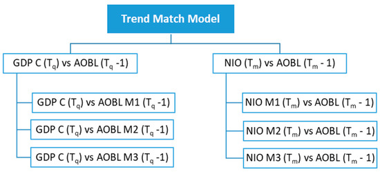
Figure 1.
Match level in models of insight 1.
The relative frequencies of trend matching for the indicators described above were achieved by first evaluating the trend (three stages) between individual periods of individual indicators (growth/stagnation/decline), after which the consensus of the development of forecast indicators AOBL and the development of GDP (C), resp. NIO 28, was evaluated in three degrees: Match (both indicator trends match), close match (indicator trends do not match in one degree), and mismatch (indicator trends do not match in two degrees).
Figure 2 provides the scheme of the trend matching breakdown in insight 1 and the overview of the time periods. The time period is an independent variable, and the trend match model is a dependent variable.
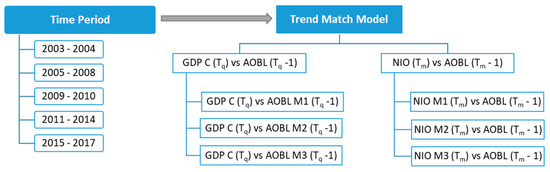
Figure 2.
Match level in models—visualization of the variables of insight 1.
Hypotheses for Insight 1:
Null hypotheses of insight 1 covered the model’s independence which meant that the result of the match is not dependent on the reference period, in other words: Match-degrees distribution (median distribution in a group) between selected business cycle indicator and subsequent economic development is consistent across the model in the reporting periods.
The specific null hypotheses for each model were:
H0(a).
Match-degrees distribution between AOBL M1 a GDP (C) is consistent across the model in the reporting periods.
H0(b).
Match-degrees distribution between AOBL M2 a GDP (C) is consistent across the model in the reporting periods.
H0(c).
Match-degrees distribution between AOBL M3 a GDP (C) is consistent across the model in the reporting periods.
H0(d).
Match-degrees distribution between AOBL a NIO 28 M1 is consistent across the model in the reporting periods.
H0(e).
Match-degrees distribution between AOBL a NIO 28 M2 is consistent across the model in the reporting periods.
H0(f).
Match-degrees distribution between AOBL a NIO 28 M3 is consistent across the model in the reporting periods.
The alternative hypothesis H1 to null hypotheses H(a–f) was that the match-degrees distribution is dependent on the reference period, resp. the distribution of medians in a group is not identical.
3.2.2. Insight 2: Match Degree across Models
In match degree across models the dependent variables were “match degrees” (match/close match/mismatch) across all the models studied and the independent variable were business cycle phases in the time period 2003–2017 (see Table 1).
Match level degrees are match, close match and mismatch. For each matching grade, its frequency was measured for all models in each period. Models with GDP (C) operated with a different frequency rate than models with NIO 28, and it was necessary to separate them.
Figure 3 provides the scheme of the match level degrees across models covered in insight 2.
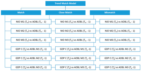
Figure 3.
Match degrees across models—visualization of the variables of insight 2.
Hypotheses for Insight 2:
Null hypotheses of insight 2 covered the models’ independence, which meant that the result of the match degree across models was not dependent on the reference period, in other words: The distribution of a match-degree of a model was the same across the monitored periods.
The specific null hypotheses for each model were:
H0(g).
The distribution of matches across GDP (C) models is the same in the monitored periods.
H0(h).
The distribution of matches across NIO 28 models is the same in the monitored periods.
H0(i).
The distribution of close matches across GDP (C) models is the same in the monitored periods.
H0(j).
The distribution of close matches across NIO 28 models is the same in the monitored periods.
H0(k).
The distribution of mismatches across GDP (C) models is the same in the monitored periods.
H0(l).
The distribution of mismatches across NIO 28 models is the same in the monitored periods.
The alternative hypothesis H1(g–l) was that the result of the match is dependent on the reference period, resp., the distribution of medians in a group is not identical.
Hypotheses Overview
The following table (Table 2) provides an overview of all hypotheses stated.
Table 2.
Null hypotheses overview.
Hypotheses Testing
In both parts of the research problem, there were categorical, explained variables (insight 1 match level in models; insight 2 match degree across models across models), and the Kruskal-Wallis test was used for hypothesis testing. It tested the assumption that the groups of variables examined could be characterized by the same median value of the explained variable, with the alternative that at least one median differed from the others [48,49].
The Kruskal-Wallis test statistics was used [49]:
where H value is [49]:
The variables in equations for insight 1: N is the total number of all measured values (match/close match/mismatch in individual models), ni is the number of values in i-th sample (per period) and Ri is the number of monitored periods.
The variables in equations for insight 2: N is the total number of all measured values (match degree across models), ni is the number of values in i-th sample (per period) and Ri is the number of monitored periods.
Next the correction for tied ranks C was solved [49]:
where g is the number of tied values, ti is the number of ties for each rank value in i-th group. After that, the test value HC could be calculated. The resulting value of HC was compared to Χ2k-1(α) value, if HC ≥ Χ2k-1(α), the null hypothesis will be rejected.
The computation was made in IBM SPSS Statistics software.
4. Results
4.1. Results for Insight 1: Match Level in Models
4.1.1. Relative Match Frequencies Based on The Models’ Results
Table 3 and Table 4 illustrate the relative frequencies of trend matching for the indicators described in Figure 1.
Table 3.
Relative match frequencies based on results of GDP models.
Table 4.
Relative match frequencies based on results of NIO 28 models.
Table 3; Table 4, which aggregate the relative trend matching frequencies, provided the following information at first glance: Predictions related to NIO 28 (see Table 4) showed a higher match rate than predictions related to GDP (C) (see Table 3) which means that more AOBL forecasts estimated the right trend of NIO 28 in the subsequent time period than the trend of GDP (C). There was also a noticeable difference between the models with different time shifts (the development within one month M1, two months M2, and three months M3 after the prediction). For GDP (C) (Table 3), the closer the forecast to monitored quarter (M3) was, the better the estimates were. With NIO 28 (Table 4), we can see that the predictions seemed most reliable (highest relative numbers in the Match column) for the following two months’ time (M2) period.
Another observed characteristic which was provided by results in Table 3; Table 4 was the distribution of the number of matches/mismatches related to the periods for which the match was evaluated. It is obvious from the Table 3; Table 4 that forecasts were best in growth periods (most in 2005–2008), specifically the models NIO 28 M2, GDP (C) M3, and NIO 28 M1). On the other hand, most of the disagreements between forecasts and economic development fell into the period of economic downturn, especially in the years 2009–2010 (in all monitored categories). These descriptive data lead to the consideration that the result of the match or reliability of the prediction depended on the economic development and the expectations of the respondents were also under its influence. This consideration was also supported by literature; see the introduction.
4.1.2. Match Level in Models Testing
The test criteria results are presented in Table 5 for insight 1.
Table 5.
Results for match level in models (insight 1).
At the significance level p = 0.05 (at Χ24(0.95) = 9.5) we did not reject any of the null hypotheses H(a–f) concerning the dependence between the match level in models and the time period. Modeled matches were not time-period-dependent. Independence could only be rejected at a significance level of p = 0.10 (at Χ24(0.90) = 7.8) for H0(e) (the NIO M2 vs. AOBL model) and adopt an alternative hypothesis that stated that the distribution of medians in the observed groups was not identical, and therefore the prediction and performance match was time-period-dependent. With a radical decrease in the significance level, it would be possible to reject the null hypothesis of other models consecutively.
4.2. Results for Insight 2: Match Degree across Models
4.2.1. Relative Match Frequencies Based on The Match Degrees
Table 6 resulted from Table 3 and Table 4 with the columns being rearranged according to the degree of matching. It still represents the relative frequencies as shown in Table 3 and Table 4. The relative frequencies were left for demonstration of the proportion of trend matching. Table 6 supported the reasoning shown by Table 3 and Table 4, namely that the result of the agreement or reliability of the prediction depends on the development of the economy, and the expectations of the respondents were under its influence.
Table 6.
Relative match frequencies based on the match degrees.
After the initial review of the Table 6, it could be found that the best matching results were in the years 2005–2008 and then 2015–2017. The worst match results were reported in the “crisis” period of 2009–2010 and also in 2011–2014. It could be summarized that the matching results in all three degrees of indicators’ agreement were consistent across the periods.
4.2.2. Match Degree across Models Testing
The test criteria results are presented in Table 7 for insight 2.
Table 7.
Results for match degree across models (insight 2).
At the significance level p = 0.05 (at Χ24(0.95) = 9.5) we did not reject any of the null hypotheses concerning the dependence between the match degree results and the time period. Modeled matches were not time-dependent. Even when the level of significance was reduced, independence could not be rejected. The distribution of matches across periods in each model was similar. The distribution of close matches across periods in each model was similar. The distribution of mismatches across periods in each model was similar. The characteristics of economic conditions at different times did not affect whether the forecast coincides with the subsequent actual developments.
5. Discussion
Routing the cash flows in companies varies according to the stage of the business cycle. These changes affect innovation significantly. In bad times, the resources shift out of the development box, and in good times, they are back there [50]. In different sectors, innovation correlates with the business cycle in varying degrees.
In times of crisis and insecurity, when the tendency to invest generally decreases [21], the importance of business cycle surveys increases. The closer to the present the indicator is, the better it can be estimated [31]. In addition to GDP data, which is published with considerable delays, there is a need to assess the current economic situation as well as the correct short-term estimate [18] for timely assessment. Future prediction models work differently; Karel and Hebák [33] argue that the "best" predictive model may change over time, for example, during different parts of the business cycle, but also for different forecast horizons [51].
Usually, financial institutions and policy-makers are the main users of these indicators. However, our analysis focuses on less frequent relation, namely the association of business cycle surveys and industrial firms. In connection with these indicators, managers of selected companies are participants in the respondents’ panel, thanks to which important development indicators are created. Yet, less is known about managers of private companies as users of these economic development indicators.
The arrival of the 2008 crisis was highly unexpected [18]. The authors have constantly been looking for the best tools to uncover future developments so that they can adapt their strategies to the new situation. For example, Reference [31] found improvements in estimation accuracy at times before turning points. Dovern and Jannsen [32] found that, in general, development is underestimated during recessions, while it is slightly overestimated in recovery periods, and, at the time of expansion, there are no systematic errors in predictions. In terms of investing in innovation during recessions, companies are making greater use of their own or local resources [4,22] while investing in new products rather than in processes. They are looking for new niches [4]. Companies that invested in the future in times of crisis were smaller firms [10] and had R&D departments before the crisis. However, these were relatively young companies (established after 2001), combining innovation with an exploration of opportunities in new markets, and their competitive strategy was product-based rather than price-based [21].
Can the influence of the period on the reliability of macroeconomic forecasts on selected indicators be confirmed? In this work, the main indicator analyzed was the assessment of order book levels (for the next 3 months) in industry. It represented the economic development forecast. The matching with subsequent reality was assessed against two different indicators at different levels of the economy. The first one was the GDP for the manufacturing sector, and the second one was the new industrial orders for a specific industrial category, namely machinery and equipment (NACE 28). This allowed us to monitor compliance with a more general scale (GDP C), but also with a major industry of the Czech economy (NIO 28). The methodology for acquiring the indicators used in the research is internationally recognized.
Forecasting and actual performance overviews (see Table 3) showed differences in forecast reliability across different models. Forecasts were compared with sector GDP (NACE C), followed by comparison with a very specific indicator—new orders in machining (NACE 28). Forecasts for the new orders provided better matching with the consequent state in a particular industry (in engineering (NACE 28)) than in sector GDP. The GDP NACE C was supposed to be better matched on account of the representativeness of the respondent’s panel (the manufacturing industry). A better prediction matching with a particular performance indicator can be explained by the nature of the chosen field of interest. Mechanical engineering (NACE 28) is an indicator of general industrial development, as the machines produced are subsequently involved in further industrial production. Furthermore, these surveys showed some imbalance in consensus at different times and, to some extent, confirmed, for example, the conclusions of Reference [32] that predictions are more reliable in times of economic growth, while less reliable during declines.
The challenge was to prove the statistical significance of this claim. By means of the non-parametric anova (Kruskall-Wallis test), it was shown that at different times the reliability did not differ significantly. If the significance level were reduced, one of the models examined would show a statistically significant period dependence, since the distribution in values varied within the groups (see Table 5). It was a model where the assessment of order book levels was compared with the development of new orders over the next two months. Another model, where dependence on the period would be demonstrated by further decreasing the significance level, was a model where the trends between assessment of book levels for the third month in a quarter and GDP for the following period were compared. These two match patterns were found to be the most matching prediction and performance ratios. When testing the distribution of data in individual model degrees (match, close match, and mismatch), significant variations in the context of different periods (see Table 6) have not been demonstrated. A cross-model test basically supported the results of deviation testing in models.
The question is how much business cycle data is actually used by businessmen. For example, Camacho et al. [30] draw attention to the fact that leading indicators research does not correspond to managers’ work. There are also indications [52] that business managers do not use these indicators sufficiently and that awareness of indicators and their use needs to be disseminated, which the author plans to verify by further research with business managers of the Czech companies belonging to NACE 28.
The impact of business cycles on the existence of companies is related to whether the company is systematically building a competitive advantage. Small businesses may connect with other small businesses and use coopetition. This can happen within clusters that help small businesses become stronger and give them the opportunity to share some know-how. The usage of presented statistical data is an innovative way of working with the information of the general environment. Such innovation helps the companies orient themselves in the market better and to be better prepared for forthcoming change.
Methods of using business cycle surveys are universal across EU countries. Business cycle surveys are harmonized for all member countries and are used in similar forms in other economies around the world. Their broader use by corporate clients, especially SMEs, is therefore a topic of sufficient importance to make the topic worth noting. Companies can work with demand estimates (and other indicators of BCS) not only in their home country, but also in foreign trade.
Future estimation influences the choice of adoption of an appropriate strategy; in other words, adjusting decisions about the future of the company. It is very useful for managers and other stakeholders to be aware of which strategies perform well at different times. One option for companies to survive business cycle fluctuations is to basically ignore the business cycle and work on innovation constantly. In difficult times, the companies should be flexible and focus on the product and the reliable after-sales service [53]. On the contrary, in times of growth, companies have enough time to prepare unconventional innovations with technological overlap into recession times [21]. These factors, in the context of an awareness of the future development of the economy, provide the company with the resilience and ability to be invulnerable and to survive difficult economic periods.
6. Conclusions
The reliability of the business cycle surveys (BCS) is constantly under investigation. The BCSs stand at the beginning of models to estimate future economic development and provide one of the most understandable indicators as it summarizes the survey responses. This makes the use of it quite attractive to managers of smaller companies. In the article, it was examined how the BCS estimates illustrate the future economic development with respect to the different phases of the economic cycle. Research has shown that at times of growth, indicators were more reliable than at times of decline.
The results are significant for all types of businesses, especially for SMEs. SMEs usually do not have a large administrative base, and the use of complicated indicators, where the manager is not able to imagine how they originated, is not very beneficial. BCSs serve to make better decisions on both tactical and strategic issues, and, especially, when deciding on future investments. The author considers it useful to present BCS indicators for their easy interpretation. Thanks to BCS, the manager can verify whether his decision would be influenced in the near future by a change in the trend of economic development.
The limitations of this study are that there is no model that predicts development completely reliably and with the same level of reliability in different parts of the business cycle. Furthermore, the use of indicators and research is based on the willingness of companies to add another item to the portfolio of information for decision making, which is not known or trusted by them. This is also the direction for further research by the author, who is going to deal with the approach of trade managers of engineering companies to the BCS indicators (do they know them, do they use them, do they consider them important?)
Author Contributions
Conceptualization, L.P.; methodology, L.P.; software, L.P.; validation, L.P.; formal analysis, L.P.; investigation, L.P.; resources, L.P.; data curation, L.P.; writing—original draft preparation, L.P.; writing—review and editing, L.P.; visualization, L.P.; supervision, L.P.; project administration, L.P.; funding acquisition, L.P.
Funding
This research was funded by the Internal Grant Agency of FaME TBU IGA/FaME/2018/001 “Leading indicators in the buying behavior of companies in B2B markets.”
Acknowledgments
The author wishes to thank the Internal Grant Agency of FaME TBU IGA/FaME/2018/001 “Leading indicators in the buying behavior of companies in B2B markets.”
Conflicts of Interest
The author declares no conflict of interest.
References
- Everett, J.; Watson, J. Small business failure and external risk factors. Small Bus. Econ. 1998, 11, 371–390. [Google Scholar] [CrossRef]
- Bhattacharjee, A.; Higson, C.; Holly, S.; Kattuman, P. Macroeconomic Instability and Business Exit: Determinants of Failures and Acquisitions of UK Firms. Econ. Lond. Sch. Econ. Political Sci. 2009, 76, 108–131. [Google Scholar] [CrossRef]
- Filippetti, A.; Archibugi, D. Innovation in times of crisis: National System of Innovation, structure, and demand. Res. Policy 2011, 40, 179–192. [Google Scholar] [CrossRef]
- Berchicci, L.; Tucci, C.L.; Zazzara, C. The influence of industry downturns on the propensity of product versus process innovation. Ind. Corp. Chang. 2013, 23, 429–465. [Google Scholar] [CrossRef]
- Paunov, C. The global crisis and firms’ investments in innovation. Res. Policy 2012, 41, 24–35. [Google Scholar] [CrossRef]
- Manso, G.; Balsmeier, B.; Fleming, L. Heterogeneous Innovation over the Business Cycle; Working Paper; University of California at Berkeley: Berkeley, CA, USA, 2017. [Google Scholar]
- Amore, M.D. Companies learning to innovate in recessions. Res. Policy 2015, 44, 1574–1583. [Google Scholar] [CrossRef]
- Saint-Paul, G. Business Cycles and Long-Run Growth. Oxf. Rev. Econ. Policy 1997, 13, 145–153. [Google Scholar] [CrossRef]
- Booz & Company. Profits Down, Spending Steady: The Global Innovation 1000. 2009. Available online: http://www.strategy-business.com/article/09404a?pg=all (accessed on 25 May 2019).
- Archibugi, D. Blade Runner Economics: Will Innovation Lead the Economic Recovery? Res. Policy 2015, 46, 535–543. [Google Scholar] [CrossRef]
- Pissourios, I.A. An interdisciplinary study on indicators: A comparative review of quality-of-life, macroeconomic, environmental, welfare and sustainability indicators. Ecol. Indic. 2013, 34, 420–427. [Google Scholar] [CrossRef]
- Giancarlo, B.; Lupi, C. Forecasting Euro-Area Industrial Production Using (Mostly) Business Surveys Data; ISAE Working Papers 33; ISTAT—Italian National Institute of Statistics: Rome, Italy, 2003. [Google Scholar]
- Bachmann, R.; Elstner, S.; Sims, E.R. Uncertainty and economic activity: Evidence from business survey data. Am. Econ. J. Macroecon. 2013, 5, 217–249. [Google Scholar] [CrossRef]
- Business Cycle Surveys—Methodology. CZSO. Available online: https://www.czso.cz/csu/czso/business_cycle_surveys (accessed on 21 January 2018).
- OECD. The Joint Harmonised EU Programme of Business and Consumer Surveys, User Guide 2017. Available online: https://ec.europa.eu/info/files/user-guide-joint-harmonised-eu-programme-business-and-consumer-surveys_en (accessed on 21 January 2018).
- Erkel-Rousse, H.; Minodier, C. Do Business Tendency Surveys in Industry and Services Help in Forecasting GDP Growth? A Real-Time Analysis on French Data; DESE Version: G2009/03; Institut National de la Statistique et des Etudes Economiques INSEE: Paris, France, 2009. [Google Scholar]
- Hansson, J.; Jansson, P.; Löf, M. Business survey data: Do they help in forecasting GDP growth? Int. J. Forecast. 2005, 21, 377–389. [Google Scholar] [CrossRef]
- Kitlinski, T. With or Without You—Do Financial Data Help to Forecast Industrial Production? Ruhr Economic Paper No. 558; SSRN: Rochester, NY, USA, 2015; pp. 1–38. [Google Scholar] [CrossRef]
- Tkacova, A.; Gavurova, B.; Behun, M. The composite leading indicator for German business cycle. J. Compet. 2017, 9, 114–130. [Google Scholar] [CrossRef]
- Srinivasan, R.; Lilien, G.L.; Sridhar, S. Should Firms Spend More on Research and Development and Advertising During Recessions? J. Mark. 2011, 75, 49–65. [Google Scholar] [CrossRef]
- Silvestri, D.; Riccaboni, M.; Della Malva, A. Sailing in all winds: Technological search over the business cycle. Res. Policy 2018, 47, 1933–1944. [Google Scholar] [CrossRef]
- Himmelberg, C.; Petersen, B. R & D and Internal Finance: A Panel Study of Small Firms in High-Tech Industries. Rev. Econ. Stat. 1994, 76, 38–51. [Google Scholar] [CrossRef]
- Tavalossi, S. Innovation determinants over industry life cycle. Technol. Forecast. 2015, 91, 18–32. [Google Scholar] [CrossRef]
- Größler, A.; Bivona, E.; Fuzhuang, L. Evaluation of asset replacement strategies considering economic cycles: Lessons from the machinery rental business. Int. J. Model. Oper. Manag. 2015, 5, 52–71. [Google Scholar] [CrossRef]
- Steenkamp, J.B.E.M.; Fang, E. The impact of economic contractions on the effectiveness of R&D and advertising: Evidence from U.S. companies spanning three decades. Mark. Sci. 2011, 30, 628–645. [Google Scholar] [CrossRef]
- Garcia-Ferrer, A.; Bujosa, M. Forecasting OECD industrial turning points using unobserved components models with business survey data. Int. J. Forecast. 2000, 16, 207–227. [Google Scholar] [CrossRef]
- Boivin, J.; Ng, S. Understanding and Comparing Factor-Based Forecasts. Int. J. Cent. Bank. 2005, 1. [Google Scholar] [CrossRef]
- Acedański, J. Forecasting industrial production in Poland—A comparison of different methods. Ekonometria 2013, 1, 40–51. [Google Scholar]
- Parigi, G.; Golinelli, R. The use of monthly indicators to forecast quarterly GDP in the short run: An application to the G7 countries. J. Forecast. 2007, 26, 77–94. [Google Scholar] [CrossRef]
- Camacho, M.; Perez-Quiros, G.; Poncela, P. Short-Term Forecasting for Empirical Economists. A Survey of the Recently Proposed Algorithms; Working Papers 1318, Banco de España, Working Papers Homepage; SSRN: Rochester, NY, USA, 2013; pp. 1–63. [Google Scholar] [CrossRef]
- Claveria, O.; Monte, E.; Torra, S. Using survey data to forecast real activity with evolutionary algorithms. A cross-country analysis. J. Appl. Econ. 2017, 20, 329–349. [Google Scholar] [CrossRef]
- Dovern, J.; Jannsen, N. Systematic errors in growth expectations over the business cycle. Int. J. Forecast. 2017, 33, 760–769. [Google Scholar] [CrossRef]
- Karel, T.; Hebák, P. Forecasting Czech GDP using Bayesian dynamic model averaging. Int. J. Econ. Sci. 2018, 7, 65–81. [Google Scholar] [CrossRef]
- Baumard, P. An asymmetric perspective on coopetitive strategies. Int. J. Entrep. Small Bus. 2009, 8, 6–22. [Google Scholar] [CrossRef]
- Bouncken, R.; Fredrich, V. Coopetition: Performance implications and management antecedents. Int. J. Innov. Manag. 2012, 16, 1–28. [Google Scholar] [CrossRef]
- Chin, K.-S.; Chan, B.L.; Lam, P.-K. Identifying and prioritizing critical success factors for coopetition strategy. Ind. Manag. Data Syst. 2008, 108, 437–454. [Google Scholar] [CrossRef]
- Angelini, E.; Camba-Mendez, G.; Giannone, D.; Reichlin, L.; Rünstler, G. Short-term forecasts of euro area GDP growth. Econom. J. 2011, 14, C25–C44. [Google Scholar] [CrossRef]
- Emerson, R.A.; Hendry, D.F. An evaluation of forecasting using leading indicators. J. Forecast. 1996, 15, 271–291. [Google Scholar] [CrossRef]
- Dovern, J. A multivariate analysis of forecast disagreement: Confronting models of disagreement with survey data. Eur. Econ. Rev. 2015, 80, 16–35. [Google Scholar] [CrossRef]
- Lemmens, A.; Croux, C.; Dekimpe, M.G. On the Predictive Content of Production Surveys: A Pan-European Study. Int. J. Forecast. 2005, 21, 363–375. [Google Scholar] [CrossRef]
- Boivin, J.; Ng, S. Are more data always better for factor analysis? J. Econ. 2006, 132, 169–194. [Google Scholar] [CrossRef]
- Hansson, J.; Jansson, P.; Löf, M. Business Survey Data: Do They Help in Forecasting the Macro Economy? Working Paper No. 84; The National Institute of Economic Research: London, UK, 2003.
- SST—Association of Engineering Technology. Report on the Machine Tools Branch in the Czech Republic in 2017. 2019. Available online: http://www.sst.cz/images/VZ_SST_2017.pdf (accessed on 21 January 2018).
- Business Cycle Surveys—Time Series. CZSO. Available online: https://www.czso.cz/documents/10180/61929913/kprcr012418_3_1.xlsx/272f05be-ba45-409a-9c04-2058b4c4d442?version=1.0 (accessed on 21 January 2018).
- Resources of Gross Domestic Product. CZSO. Available online: https://www.czso.cz/documents/10180/46120889/hdpcr011018_z.xlsx/ce0c8f6a-6b02-4c48-9674-28c45644c3f0?version=1.0 (accessed on 21 January 2018).
- New Industrial Orders—Year-on-YEAR indices. CZSO. Available online: https://www.czso.cz/documents/10180/91839483/prucr040819_13.xlsx/33cc8d16-83c9-4b77-8544-a26d37748d36?version=1.0 (accessed on 21 January 2018).
- Statistical Classification of Economic Activities in the European Community, Rev. 2. Eurostat. 2008. Available online: https://ec.europa.eu/eurostat/ramon/nomenclatures/index.cfm?TargetUrl=LST_NOM_DTL&StrNom=NACE_REV2&StrLanguageCode=EN (accessed on 21 January 2018).
- Řezanková, H. Analýza dat z dotazníkových šetření (Data Analysis from Survey), 2nd ed.; Professional Publishing: Praha, Czech Republic, 2010; pp. 105–107, 156–157. [Google Scholar]
- Guo, S.; Zhong, S.; Zhang, A. Privacy-preserving Kruskal-Wallis test. Comput. Methods Programs Biomed. 2013, 112, 135–145. [Google Scholar] [CrossRef] [PubMed]
- Devinney, T.M. New products over the business cycle. J. Prod. Innov. Manag. 1990, 7, 261–273. [Google Scholar] [CrossRef]
- Berge, T.J. Predicting Recessions with Leading Indicators: Model Averaging and Selection over the Business Cycle; Federal Reserve Bank of Kansas City Working Paper; No. 13-05; Federal Reserve Bank of Kansas City: Kansas City, MO, USA, 2014.
- Manažerské shrnutí výsledků metodického auditu statistiky ČSÚ (The Summary of Methodic Audit of ČSÚ Statistics for Mangers). CZSO. Available online: https://www.czso.cz/documents/10180/39785642/audit_8.pdf/8b6faf27-d983-42c9-afbc-1c4c35a7263e?version=1.1 (accessed on 21 January 2018).
- Lorentz, H.; Hilmola, O.P.; Malmsten, J.; Srai, J.S. Cluster analysis application for understanding SME manufacturing strategies. Expert Syst. Appl. 2016, 66, 176–188. [Google Scholar] [CrossRef]


© 2019 by the author. Licensee MDPI, Basel, Switzerland. This article is an open access article distributed under the terms and conditions of the Creative Commons Attribution (CC BY) license (http://creativecommons.org/licenses/by/4.0/).