Abstract
As photovoltaic (PV) power plants are an essential component of modern smart grids, the PV generation forecasting of such plants has recently been gaining interest. The forecasting results of PV power often suffer from large errors because of unusual weather conditions. In a learning-based forecasting model, the forecasting accuracy can be enhanced by using carefully selected data for training rather than all the data without any screening. That is, using a training set that only contains information obtained from similar days can help enhance the accuracy of learning-based PV forecasting. This paper proposes a forecasting method for small-scale PV generation. This method is based on long short-term memory; further, it detects similar days considering the different impacts of weather variables on PV power according to the day. This method can address issues caused by unnecessary learning from non-similar historical days. The simulation results demonstrate that the proposed method exhibits better performance than do existing similar day detection methods.
1. Introduction
Photovoltaic (PV) power has attracted significant attention as an emission-free power source owing to increasing awareness about global warming. However, as more PV generators are integrated into power systems, uncertain and non-dispatchable PV power causes difficulties in the power systems [1,2]. In particular, several small-scale PV generators that are integrated in a distribution grid make it considerably difficult to maintain the operational security of the power systems. To address this issue, the accuracy of short-term forecasting models for PV power should be enhanced.
As PV power is largely dependent on weather conditions, most studies on short-term PV power forecasting (STPPF) are based on the data of predicted weather conditions [3]. Recent STPPF models can be categorized into statistical, learning-based, and hybrid techniques. In the statistical approach, PV power is treated as a time series, and past observations of PV power are used statistically by process models such as the vector auto-regression model [4], ordinary least square model [4], gradient boosting [4], extreme learning machine [5,6], empirical mode decomposition [6], and sine cosine algorithm [5]. Seasonal modeling and weather information are crucial for these approaches due to the characteristics of PV power fluctuations [7]. Owing to advancements in learning-based algorithms, many STPFF models [8,9,10,11,12] have started using learning-based research. They can be further classified into machine-learning- and deep-learning-based approaches. Support vector regression (SVR) [8] and artificial neural networks (ANNs) [9] are perfect examples of the machine-learning-based approach that can provide better performance even with few recorded datasets. Back-propagation neural networks (BPNNs) [10,11,12] and long short-term memory (LSTM) networks [13,14] represent deep-learning-based approaches, and they exhibit considerably better performance when several datasets are used in the training process. However, a BPNN has a higher chance to get stuck in local minima, and LSTM entirely depends upon the type of input PV training data even when the amount of input PV data is sufficiently large. Due to these issues, these forecasting methodologies deliver an average normalized mean absolute error (nMAE) in the range of 10–25%. Such problems are because the PV power changes with the weather conditions [15]. Therefore, the training set contains unnecessary data.
To address the potential problems of overfitting and underfitting, a few hybrid STPPF models have been developed [16,17,18,19,20,21,22,23]. In the hybrid approach, a specific type of day is detected, and then similar days are identified. The specific types of days are defined in PV power forecasting mostly based on weather conditions described in colloquial language, such as sunny, rainy, and cloudy days [16,17]. Moreover, some studies used numerical weather predictions (NWPs) to define similar days. In [15], two important variables were selected based on Euclidean distance (ED) to detect similar days. Statistical models such as statistical analysis software (like SPSS) [16], discrete wavelet transformation (DWT) [18], radial basis function [19], and wavelet packet distribution (WPD) [20] have also been used to define a specific type of day. Furthermore, learning-based clustering techniques such as support vector machine (SVM) [17], k-nearest neighbors (k-NN) [17], and self-organizing maps (SOMs) classification [21,22] have also been applied to extract similar weather days. The common goal for all these hybrid techniques is to seek similar days from historical data and, eventually, to create a new PV series for better training results. Consequently, these methodologies have an average forecasting nMAE of around 5–18%, merely depending upon a type of day. However, they still fail to effectively disclose daily forecasting results.
Although several methods have been developed in existing studies, an accurate method of similar day detection in PV power forecasting still remains undiscovered because different weather variables have different relationships with PV power generation. Some weather variables are highly correlated to the PV power and, hence, provide important information for accurate PV forecasting for all day types. However, other weather variables are correlated to the PV power only for certain day types. In other words, these variables provide important information to increase the forecasting accuracy for some days; however, they may cause overfitting problems for other days. That is, the impacts of weather variables on PV generation change as the type of a specific day is varied, and the most informative weather variables vary daily. Thus, to enhance the accuracy of learning-based PV forecasting, a proper training set should be developed that only contains information obtained from similar days considering the different impacts of weather variables on PV power for each day type.
This paper proposes a similar day detection (SDD) method for learning-based PV forecasting that deals with different impacts of weather variables on PV power for each day type. The proposed similar day detection method first classifies historical days into several groups by considering the similarity of PV power patterns. In addition, important weather variables are selected for each day type considering their different impacts on the PV power. Finally, a new PV series is created from the identified similar days, which is more repetitive and appropriate for the LSTM-based PV forecasting model.
2. Weather’s Impact on PV Power Forecasting
Several weather variables can be used for PV forecasting, such as temperature, humidity, wind speed, rain amount, daylight hours, and cloud cover. Further, different weather variables have different relationships with PV generation. Figure 1 shows the Pearson correlation coefficients between historical PV power and selected weather variables. In Figure 1, the correlation of each weather variable is changing day by day. For example, the average temperature is positively correlated to PV power on Day 1 and Day 4. In contrast, for Day 5 and Day 6, it is negatively correlated to PV power. These observations show the complicated and inconsistent relationship between PV power and weather variables. Figure 2 shows the distribution of the selected weather variables according to PV power, as observed in the southern region of Korea in 2015.
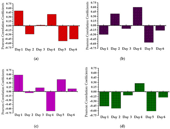
Figure 1.
Correlation coefficients between photovoltaic (PV) power and weather variables: (a) average temperature, (b) rain amount, (c) daylight hours, and (d) cloud cover.
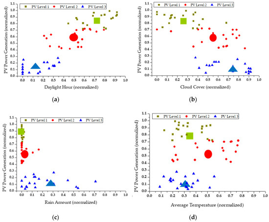
Figure 2.
Distribution of weather variables according to PV power: (a) daylight hours, (b) cloud cover, (c) rain amount, and (d) average temperature.
In Figure 2, the historical data are classified into different colored dots denoting three levels of PV power. As weather variables values are increased, the PV power tends to increase or decrease as shown in Figure 2a,b, respectively. The varying information from these weather variables is closely linked to the PV power for all generation levels. Hence, these variables can be used as an index to identify the types of days for all periods. In contrast, in Figure 2c,d, some weather variables show an influence on PV power only on days of a certain level of PV generation, and these weather variables provide some information of diversity and randomness on these days. Although these weather variables present complexity and uncertainty, they help deliver similar weather information for days of a certain level of PV generation.
For SDD, the following two types of weather variables for each day group, classified based on the PV power pattern, should be identified. One variable is highly correlated to the PV power and, hence, can be used for primary sorting to select groups of similar days. The other variables have some information only for day types with a specific generation pattern. Because these variables can interfere with the PV prediction of specific days, they should be selected by day group and used for secondary sorting to select similar days. Figure 3a,b describes the conventional method and proposed SDD method, respectively. To consider the impact of weather variables by PV power patterns, historical days are classified into several groups by their PV patterns, and different weather variables are used for each group of days to estimate their similarity to the target day. With this proposed strategy for detecting similar days, the training set is expected to contain the PV patterns of many similar days so that the forecasting model can provide more accurate results. The proposed similar day detection strategy is described in the following section.
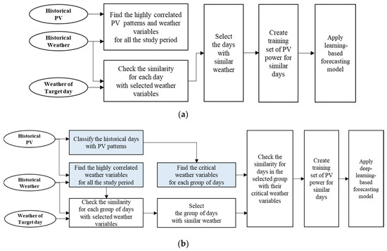
Figure 3.
Overview of similar day detection strategies: (a) conventional method and (b) proposed method.
3. Proposed Short-Term PV Power Forecasting
3.1. Classification of Days with Historical PV Generation
To reduce the probability of overfitting and underfitting problems in the learning-based forecasting model, the training set needs to be reduced so that it contains the generation patterns of days with similar PV generation and weather conditions. As the first step of selecting similar days, historical days are classified by considering the similarity of generation patterns. The historical generation pattern of PV power can be expressed as follows:
where vector is the hourly generation profiles of PV power on day d, and D represents the number of days of historical data.
To classify the days with similar historical generation patterns, a self-organizing map (SOM) and learning vector quantization (LVQ) based algorithm [24,25,26] is used in this study, which is a semi-supervised classification technique. The SOM and LVQ algorithm selects the closest node which represents the closest day for among the randomly distributed nodes . This algorithm then iteratively updates the closest node and explores the corresponding neighbors. The closest node is selected by the competitive learning rule of minimum Euclidean distance as follows:
Once the clustering model is sufficiently trained for all days d, each input is mapped into k different groups as an output. For each kth PV group, similar types of PV power generation are collected and can be mapped into group :
where is the number of similar PV power generation days for the clustering output PV group k. With this clustering, the historical days that have a similar generation pattern are classified into group k. Further, the historical NWPs of the days that belong to group k are defined as follows:
where is the numerical prediction value of weather variable j on day d that belongs to group k; and J are the number of days that belong to group k and the number of weather variables to be considered, respectively. For developing , various weather variables such as temperature, wind speed, rain amount, humidity, cloud cover, and daylight hours can be used.
3.2. Decomposition of Weather Variables
In this study, based on their relationship with PV generation, weather variables are classified into two types: primary weather variables (PWVs) and secondary weather variables (SWVs). The PWVs are highly correlated to PV generation for all days. PV generation can change greatly due to these variables as the difference in PWV values among the day groups is higher than that for the other weather variables. In contrast, the SWVs are correlated to PV generation only in a certain day group k. These variables give important information that increases the forecasting accuracy for some days; however, they cause overfitting issues in learning-based forecasting for other days.
Because of the high correlation between the PWVs and PV generation, there should be a high deviation between the day groups that are classified by the PV generation pattern. In this study, to identify the PWVs of a PV site, the deviations of each variable are estimated, and the variables of higher deviation are selected as PWVs. The deviation of variable j is calculated as the difference between the minimum and maximum averages of as follows:
where is the deviation of variable j and is the average value of weather variable in day group k. The average value in Equation (5) can be calculated as follows:
By using this deviation between the day groups, the weather variables with higher deviation () are selected as PWVs as follows:
where is the set of indices of PWVs, and is the PWV threshold used to select higher . Figure 4 shows an example distribution of weather variables’ averages by day group.
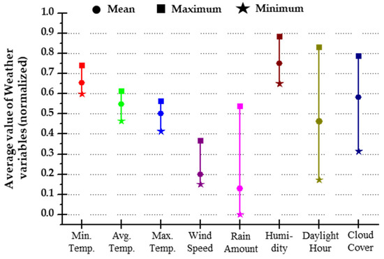
Figure 4.
Example distribution of weather variables averaged by day group.
In contrast, SWVs cannot provide the information needed to recognize huge changes in PV generation. Therefore, the deviation of SWV values among the day groups is less than that of PWVs. Although SWVs can increase the forecasting accuracy for some days, extension of the training set tends to give better results in learning-based methods. Since SWVs can cause overfitting in learning-based forecasting for some days, adequate SWVs should be selected for a certain day group k. This study estimates the deviations of each variable, and the variables with higher deviation are selected as the SWVs for a certain day group k. This is similar to the selection of PWVs; however, it is different in that it estimates the deviation of weather variables within a day group. The deviation of variable j for day group k is calculated as follows:
The weather variables with higher deviation () are SWVs, and they help further divide the day group. The SWVs for day group k are selected as follows:
where is the set of indices of SWVs of day group k and is the SWV threshold to select higher .
3.3. Detection of Similar Days
The weather variables with higher can give primary information to select similar days. With the similarity of PWVs, a similar day group k can be selected as follows:
where is the forecasting value of variable j for the forecasting day. A similar day group k selected using Equation (10) includes days with similar PV generation and PWVs. However, similarity of all the days in the selected group k is not sufficient to increase the forecasting accuracy, because diversities of weather variables still exist in these days. To solve this problem, the SWVs can help us to identify the most similar days within the selected group k. For selecting the most similar days, the similarity of SWVs is estimated for the days in the selected group k as follows:
where is the similarity between the SWVs of days in group k and the forecasting day. When a day has lower , the SWVs of the day are much closer to those of the forecasting day. Finally, only the profiles of the days with lower are used as the training set ,
where is the constant threshold to select higher . Using Equation (12), the most similar days are detected and collected in .
3.4. LSTM-Based Day-Ahead PV Power Forecasting
The long short-term memory (LSTM) approach, one of the best versions of recurrent neural networks, can learn temporal relationships in a time series. Since the LSTM learning process has the ability to understand relationships among distant dependencies [27], the LSTM methodology is useful when the input sequential series contains a lot of repetitive patterns [13,20]. The PV generation of Equation (12) behaves as a strong stationary time series [28]. Therefore, it is more suitable for the LSTM network than the conventional PV generation series.
Figure 5 shows the structure of the training and testing sets of the proposed LSTM-based architecture. In Figure 5, series of PV generation on the selected similar days are expressed via elements . In the training set , the selected time series of similar days is used instead of the original time series () of PV generation. With this selection of training data, overfitting in the learning network can be mitigated so that the forecasting accuracy for PV generation can be improved.
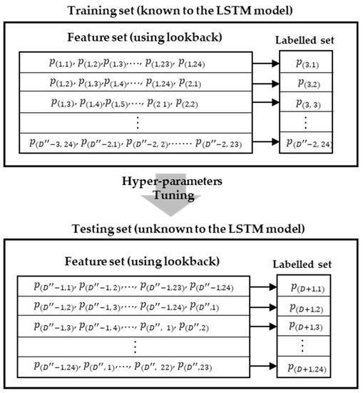
Figure 5.
Structure of the training and testing data for the proposed method.
For the LSTM network, the weight and bias of the forget, input, and output gates are updated in the form of gradient error signals. In addition, the input temporal patterns forming error signals link the appropriate values of PV generation after a certain time t through the gates and sigmoid activation functions. The forget gate controls which information needs to be forgotten from the previous cell state. The input gate decides which information needs to be updated in the cell state, and the output gate sends the right cell state as the output. To optimize the LSTM model, a root mean square is used for the training process as follows:
where is the number of similar days, which is the length of the training set, and is the predicted PV generation obtained from the LSTM. Figure 6 illustrates the procedure for the proposed PV generation forecasting.
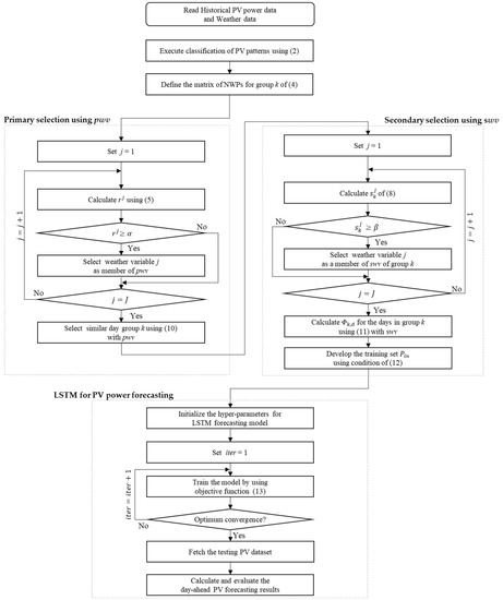
Figure 6.
The overall procedure of the proposed PV power forecasting method.
4. Numerical Results and Discussion
4.1. PV Data Description and Implementation
The proposed method was tested using hourly recorded data gathered from a 1 MW PV site in Goheung, Korea, for one year (January 2015 to December 2015). The daily measurement of weather data is forecasted and announced by the Metrological Administration of South Korea. Most of the weather data were used without any modification. However, rain amount data of more than 50 mm were changed to 50 mm because PV generators are expected not to produce electrical power when the daily rain amount is more than 50 mm. Table 1 presents sample data of the eight daily weather variables that were used for the numerical simulation. Also, Table 2 presents the technical specifications of the PV power plants.

Table 1.
Weather data used in the numerical simulation.
Table 2.
Technical specifications of the photovoltaic (PV) system.
With the consideration of seasonal impact and data requirement issues [11,16,29], the training dataset was developed using the latest six-month data. Hence, for each time, the training dataset comprised PV data and NWPs of 180 days. Using this dataset, the results of the proposed method were compared with the results of [16,29] as well as with the results of other deep learning models [11,13,20]. The training simulation was performed in a Windows operating system on an I7-6700 CPU at 3.40 GHz with 16 GB installed RAM.
To evaluate the accuracy of forecasting results, we employed the normalized mean absolute percentage error (nMAE) and root-mean-square error (RMSE), which are calculated as follows:
where is the forecasting PV power at time t; is the actual PV power at time t; and is the generation capacity of the PV site.
For clustering the PV power, the number of groups was set to be 6. To explore the PWVs and SWVs, thresholds and were both set to 0.5. The PV series that was extracted from the similar days was tested via Tensor-flow (backend), where the frontend was Python with the Keras library [30]. The tuning process of the appropriate hyper-parameters was inspired by [31,32,33,34,35]. The common hyper-parameters, such as the number of hidden layers, activation function, optimization algorithm, and number of nodes per layer, are summarized in Table 3. The additional hyper-parameters were set as follows: inner activation function was hard sigmoid, monitor function was validation loss, patience size was 3, and drop-out was 0.5. The fully connected layer was attached to the output layer of the LSTM. Each time, one-hour predicted PV power values were obtained from the fully connected layer. The dataset was split into a validation set (3 days), testing set (1 day), and training set (remaining days) for each day of the week.
Table 3.
Hyper-parameters for selected models.
4.2. Results of Day-Ahead PV Forecasting
Figure 7 and Table 4 show the forecasting results with and without the proposed similar day detection method for a few selected weeks (peak load season of Korea). For the cases without the proposed similar day detection, forecasting models based on SVR, BPNN, and LSTM were tested, and each network was trained via back-propagation with mean squared error as the loss function. Figure 7 shows that the forecasting results with the proposed method are generally closer to the actual PV power than others. As summarized in Table 4, by using the proposed similar day detection, the average nMAE and average RMSE were improved by a minimum of 2% and 20 kWh, respectively. Thus, in conclusion, the proposed forecasting method can significantly improve the forecasting accuracy when compared to other forecasting models without similar day detection.
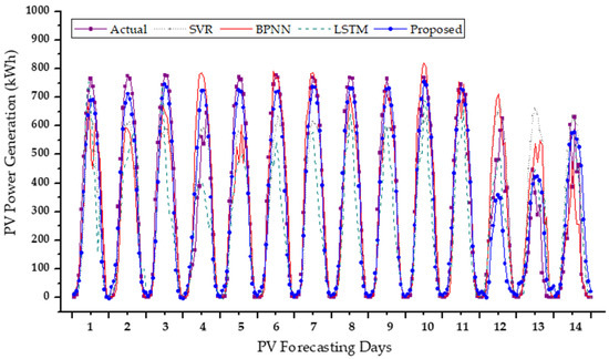
Figure 7.
Results of PV power forecasting with and without the proposed similar day detection (SDD).
Table 4.
Normalized mean absolute error (nMAE) and root-mean-square error (RMSE) of PV power forecasting with and without the proposed similar day detection (SDD).
For each testing day, the computational times for the similar day detection and LSTM networks were about 2 minutes and 15 minutes, respectively. The entire computational time of the proposed hybrid technique was substantially lower than that of the conventional LSTM-based network.
4.3. Comparison with Existing SDD Models
This section compares the results of the proposed similar day detection and two other similar day detection methods (SDD-A and SDD-B). The similar day detection methods SDD-A and SDD-B were built by referring to [9,21,29], respectively. To check the efficacy of the proposed similar day detection method, we arbitrarily picked four weeks each in the summer, autumn, and winter seasons.
Figure 8 shows the daily average nMAE and RMSE of the proposed PV power forecasting for the four selected weeks of each season. On most days, the proposed forecasting method significantly improved the forecasting accuracy when compared to SDD-A and SDD-B. The forecasting nMAE and RMSE are often varied because the type of day can vary day by day. This is because forecasting performance depends not only on weather conditions but also on the collection of most similar days and the hyper-parameter tuning process of the LSTM network.
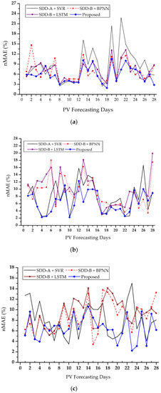
Figure 8.
Daily normalized mean absolute error (nMAE) and root-mean-square error (RMSE) of PV power forecasting with different SDD methods. (a) Summer, (b) autumn, and (c) winter.
Table 5 shows the weekly average nMAE and RMSE of PV power forecasting for the four selected weeks of each season. In summer, the proposed model reported a 5.86% nMAE, which was lower than SDD-B (with BPNN) with a 6.94% nMAE. In autumn, when the PV generation level is higher, the proposed model reported a 6.43% nMAE, which was lower than SDD-A (with SVR) with a 7.85% nMAE. Similarly, in winter, when the PV generation level is lower, the proposed model reported a 6.60% nMAE, which was lower than SDD-A (with SVR) with an 8.16% nMAE. The summary in Table 5 shows that the proposed method improved the forecasting accuracy by about 2 percent throughout the study period. A similar level of improvement was seen while evaluating the performance of forecasting using the RMSE metric. Thus, the evaluation demonstrates that the PV forecasting model can deliver better performance by training only with data from the proposed similar day detection.
Table 5.
Weekly nMAE and RMSE of PV power forecasting with different SDD methods.
4.4. Impact of
Figure 9 shows the PV forecasting results with different values for selected weeks of summer, autumn, and winter. In the summer and autumn seasons, more accurate forecasting can be expected when the parameter is set to be around 1.7. However, in the winter season, more accurate forecasting can be expected with the parameter set to be around 1.6, which is lower than the cases of summer and autumn. The higher value of provides more training data to the LSTM, so that the LSTM has a greater chance to learn the PV characteristics, However, more training data can increase internal variance in the training set, which can cause overfitting of the hyper-parameters of the LSTM, degrading the optimal learning of the LSTM. Therefore, it is necessary to explore the optimal value as it can vary with seasonal weather conditions.
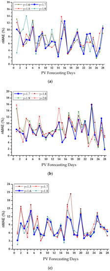
Figure 9.
Results of PV power forecasting with different values. (a) Summer, (b) autumn, and (c) winter.
5. Conclusions
In this paper we proposed a forecasting method for small-scale PV generation based on LSTM combined with a similar day detection method that considers the different impacts of weather variables on PV power by day type. In the proposed method, important weather variables are selected for each day group that is classified by considering the similarity of PV power patterns. With the selected weather variables, this method identifies similar days which are repetitive and thus appropriate to the LSTM-based PV forecasting model. By using the proposed method, forecasting accuracy for small-scale PV generation can be improved. The test results indicated that the proposed method can deliver a notable improvement by training solely with data obtained from similar days. This method can be used for operation of a distribution grid with accurate forecasting of distributed PV generation. In future work, this study will be extended to very-short-term PV power forecasting by including more weather parameters and by considering the relationships between the physical characteristics of PV generators and weather variables.
Author Contributions
For this research, S.K.A. developed the idea of PV forecasting framework, performed the simulation, and wrote the paper. Y.-M.W. helped organize the article. J.L. provided guidance for the research and revised the paper. All authors have read and agreed to the published version of the manuscript.
Funding
This work was supported by the National Research Foundation of Korea (NRF) grant funded by the Korea government (MSIT) (No. 2019R1H1A1080137). This research was also supported by Korea Electric Power Corporation (Grant number: R18XA04).
Conflicts of Interest
The authors declare no conflict of interest.
References
- Cohen, M.A.; Callaway, D.S. Effects of Distributed PV Generation on California’s Distribution System, Part 1: Engineering Simulations. Sol. Energy 2016, 128, 126–138. [Google Scholar] [CrossRef]
- Woyte, A.; Van Thong, V.; Belmans, R.; Nijs, J. Voltage Fluctuations on Distribution Level Introduced by Photovoltaic Systems. IEEE Trans. Energy Convers. 2006, 21, 202–209. [Google Scholar] [CrossRef]
- Das, U.K.; Tey, K.S.; Seyedmahmoudian, M.; Mekhilef, S.; Idris, M.Y.I.; Van Deventer, W.; Horan, B.; Stojcevski, A. Forecasting of Photovoltaic Power Generation and Model Optimization: A review. Renew. Sustain. Energy Rev. 2018, 81, 912–928. [Google Scholar] [CrossRef]
- Bessa, R.J.; Trindade, A.; Miranda, V. Spatial Temporal Solar Power Forecasting for Smart Grids. IEEE Trans. Ind. Inform. 2014, 3203, 232–241. [Google Scholar] [CrossRef]
- Wan, C.; Lin, J.; Song, Y.; Xu, Z.; Yang, G. Probabilistic Forecasting of Photovoltaic Generation: An Efficient Statistical Approach. IEEE Trans. Power Syst. 2017, 32, 2471–2472. [Google Scholar] [CrossRef]
- Behera, M.K.; Nayak, N. A Comparative Study on Short Term PV Power Forecasting Using Decomposition Based Optimized Extreme Learning Machine Learning Algorithm. Eng. Sci. Technol. Int. J. 2019, 23, 156–167. [Google Scholar] [CrossRef]
- Han, Y.; Wang, N.; Ma, M.; Zhou, H.; Dai, S.; Zhu, H. A PV Power Interval Forecasting Based on Seasonal Model and Nonparametric Estimation Algorithm. Sol. Energy 2019, 184, 515–526. [Google Scholar] [CrossRef]
- Alfadda, A.; Adhikari, R.; Kuzlu, M.; Rahman, S. Hour-Ahead Solar PV power forecasting Using SVR Based Approach. In Proceedings of the 2017 IEEE Power & Energy Society Innovative Smart Grid Technologies Conference (ISGT), Washington, DC, USA, 23–26 April 2017; pp. 1–5. [Google Scholar]
- Li, Z.; Rahman, S.M.; Vega, R.; Dong, B. A Hierarchical Approach Using Machine Learning Methods in Solar Photovoltaic Energy Production Forecasting. Energies 2016, 9, 55. [Google Scholar] [CrossRef]
- Ding, M.; Wang, L.; Bi, R. An ANN-Based Approach for Forecasting the Power Output of Photovoltaic System. Procedia Environ. Sci. 2011, 11, 1308–1315. [Google Scholar] [CrossRef]
- Hu, Y.; Lian, W.; Dai, S.; Zhu, H. A Seasonal Model Using Optimized Multi-Layer Neural Networks to Forecast Power Outputs of PV Plants. Energies 2018, 11, 326. [Google Scholar] [CrossRef]
- Huang, C.; Cao, L.; Peng, N.; Li, S.; Zhang, J.; Wang, L.; Luo, X.; Wang, J. Day-Ahead Forecasting of Hourly Photovoltaic Power Based on Robust Multilayer Perceptron. Sustainability 2018, 10, 4863. [Google Scholar] [CrossRef]
- Jung, Y.; Jung, J.; Kim, B.; Han, S. Long Short-Term Memory Recurrent Neural Network for Modelling Temporal Patterns in Long-Term Power Forecasting for Solar PV Facilitates: Case Study of South Korea. J. Clean. Prod. 2020, 250, 119476. [Google Scholar] [CrossRef]
- Lee, D.; Kim, K. Recurrent Neural Network-Based Hourly Prediction of Photovoltaic Power Output Using Meteorological Information. Energies 2019, 12, 215. [Google Scholar] [CrossRef]
- Zhang, Y.; Beaudin, M.; Taheri, R.; Zareipour, H.; Wood, D. Day-Ahead Power Output Forecasting for Small-Scale Solar Photovoltaic Electricity Generators. IEEE Trans. Smart Grids 2015, 6, 2253–2262. [Google Scholar] [CrossRef]
- Cheng, K.; Guo, L.M.; Zafar, M.T. Application of Clustering Analysis in the Prediction of Photovoltaic Power Generation Based on Neural Network. IOP Conf. Ser. Earth Environ. Sci. 2017, 93, 012024. [Google Scholar] [CrossRef]
- Wang, F.; Zhen, Z.; Wang, B.; Mi, Z. Comparative Study on KNN and SVM Based Weather Classification Models for Day Ahead Short-Term Solar PV Power Forecasting. Appl. Sci. 2018, 8, 28. [Google Scholar] [CrossRef]
- Nazaripouya, H.; Wang, B.; Wang, Y.; Chu, P.; Pota, H.R.; Gadh, R. Univariate Time Series Prediction of Solar Power Using a Hybrid Wavelet-ARMA-NARX Prediction Method. In Proceedings of the 2016 IEEE/PES Transmission and Distribution Conference and Exposition (T&D), Dallas, TX, USA, 3–5 May 2016; pp. 1–5. [Google Scholar]
- Lu, H.J.; Chang, G.W. A Hybrid Approach for Day-ahead Forecast of PV power Generation. Int. Fed. Autom. Control-Pap. Online 2018, 51, 634–638. [Google Scholar] [CrossRef]
- Li, P.; Zhou, K.; Lu, X.; Yang, S. A Hybrid Deep Learning Model for Short-Term PV Power Forecasting. Appl. Energy 2019, 259, 114216. [Google Scholar] [CrossRef]
- Yang, H.T.; Huang, C.M.; Huang, Y.C.; Pai, Y.S. A Weather-Based Hybrid Method for 1-day Ahead Hourly Forecasting of PV Power Output. IEEE Trans. Sustain. Energy 2014, 5, 917–926. [Google Scholar] [CrossRef]
- Dong, Z.; Yang, D.; Reindl, T.; Walsh, W.M. A Novel Hybrid Approach Based on Self-Organizing Maps, Support Vector Regression and Particle Swarm Optimization to Forecast Solar Irradiance. Energy 2015, 82, 570–577. [Google Scholar] [CrossRef]
- Massucco, S.; Mosaico, G.; Saviozzi, M.; Silvestro, F. A Hybrid Technique for Day-Ahead PV Generation Forecasting Using Clear-Sky Models or Ensemble of Artificial Neural Networks According to a Decision Tree Approach. Energies 2019, 12, 1298. [Google Scholar] [CrossRef]
- Kohonen, T. The Self-Organizing Maps. Proc. IEEE 1990, 78, 1464–1480. [Google Scholar] [CrossRef]
- Kohonen, T. Essentials of the self-organizing map. Neural Netw. 2013, 37, 52–65. [Google Scholar] [CrossRef] [PubMed]
- Chang, L.-C.; Amin, M.Z.M.; Yang, S.-N.; Chang, F.-J. Building ANN-Based Regional Multi-Step-Ahead Flood Inundation Forecast Models. Water 2018, 10, 1283. [Google Scholar] [CrossRef]
- Pattanayek, S. Pro Deep Learning with TensorFlow: A Mathematical Approach to Advanced Artificial Intelligence in Python, 1st ed.; Apress: New York, NY, USA, 2017; pp. 223–251. [Google Scholar]
- Box, G.E.P.; Jenkins, G.M.; Reinsel, G.C.; Ljung, G.M. Time Series Analysis: Forecasting and Control, 5th ed.; John Wiley & Sons: Hoboken, NJ, USA, 2015; pp. 21–176. [Google Scholar]
- Xu, R.; Chen, H.; Sun, X. Short-Term Photovoltaic Power Forecasting with Weighted Support Vector Machine. In Proceedings of the IEEE International Conference on Automation and Logistics (ICAL), Zhengzhou, China, 15–17 August 2012. [Google Scholar]
- Pedregosa, F.; Varoquax, G.; Gramfort, A. Scikit-learn: Machine Learning in Python. J. Mach. Learn. Res. 2011, 12, 2825–2830. [Google Scholar]
- Zhang, W.; Quan, H.; Srinivasan, D. An Improved Quantile Regression Neural Network for Probabilistic Load Forecasting. IEEE Trans. Smart Grid 2019, 10, 4425–4434. [Google Scholar] [CrossRef]
- Ogliari, E.; Niccolai, A.; Leva, S.; Zich, R.E. Computational Intelligence Techniques Applied to the Day Ahead PV Output Power Forecast: PHANN, SNO and Mixed. Energies 2018, 11, 1487. [Google Scholar] [CrossRef]
- Ozaki, Y.; Yano, M.; Onishi, O. Effective Hyper-Parameter Optimization using Nelder–Mead Method in Deep Learning. PSJ Trans. Comput. Vis. Appl. 2017, 9, 20–25. [Google Scholar] [CrossRef]
- Acharya, S.K.; Min, Y.M.; Lee, J. Short-term Load Forecasting for a Single Household Based on Convolution Neural Networks Using Data Augmentation. Energies 2019, 12, 3560. [Google Scholar] [CrossRef]
- Kim, J.; Cho, S.B. Evolutionary Optimization of Hyper-parameters in Deep Learning Models. In Proceedings of the 2019 IEEE Congress on Evolutionary Computation (CEC), Wellington, New Zealand, 10–13 June 2019. [Google Scholar]


© 2020 by the authors. Licensee MDPI, Basel, Switzerland. This article is an open access article distributed under the terms and conditions of the Creative Commons Attribution (CC BY) license (http://creativecommons.org/licenses/by/4.0/).