Article

SR-SYBA: A Scale and Rotation Invariant Synthetic Basis Feature Descriptor with Low Memory Usage

1
School of Electronics and Information Technology, Sun Yat-sen University, Guangzhou 510006, China
2
Department of Electrical and Computer Engineering, Brigham Young University, Provo, UT 84602, USA
3
Cubiscan, Inc., Farmington, UT 84025, USA
*
Author to whom correspondence should be addressed.
Electronics 2020, 9(5), 810; https://doi.org/10.3390/electronics9050810
Submission received: 28 March 2020 / Revised: 10 May 2020 / Accepted: 12 May 2020 / Published: 15 May 2020
(This article belongs to the Special Issue Convolutional Neural Networks and Vision Applications)

Abstract

:
Feature description has an important role in image matching and is widely used for a variety of computer vision applications. As an efficient synthetic basis feature descriptor, SYnthetic BAsis (SYBA) requires low computational complexity and provides accurate matching results. However, the number of matched feature points generated by SYBA suffers from large image scaling and rotation variations. In this paper, we improve SYBA’s scale and rotation invariance by adding an efficient pre-processing operation. The proposed algorithm, SR-SYBA, represents the scale of the feature region with the location of maximum gradient response along the radial direction in Log-polar coordinate system. Based on this scale representation, it normalizes all feature regions to the same reference scale to provide scale invariance. The orientation of the feature region is represented as the orientation of the vector from the center of the feature region to its intensity centroid. Based on this orientation representation, all feature regions are rotated to the same reference orientation to provide rotation invariance. The original SYBA descriptor is then applied to the scale and orientation normalized feature regions for description and matching. Experiment results show that SR-SYBA greatly improves SYBA for image matching applications with scaling and rotation variations. SR-SYBA obtains comparable or better performance in terms of matching rate compared to the mainstream algorithms while still maintains its advantages of using much less storage and simpler computations. SR-SYBA is applied to a vision-based measurement application to demonstrate its performance for image matching.

1. Introduction

The process of image matching looks for corresponding targets in two images by analyzing the similarity and consistency of image contents, structures, features, relationships, textures and gray scales [1]. Image matching plays an important role in many computer vision tasks, e.g., target tracking, object detection, and visual petitioning. Image matching techniques can be categorized into intensity-based and feature-based [2]. Intensity-based matching methods regard the image as a two-dimensional signal and look for possible matching feature points using statistical means to evaluate the similarity between the two image signals. Feature-based matching methods describe the characteristics of images with high-level features, e.g., color, texture, space position, and shape, and find correspondences by performing a matching process among the features. Compared with intensity-based methods, feature-based matching methods are more robust to image perturbations including image compression artifacts, illumination change, blurring, and perspective transformation [2].
Feature detection, feature description, and feature matching are three basic steps for feature-based image matching methods [3]. As the key to feature-based image matching algorithms, feature description characterizes a small region surrounding the detected feature points in the image. A good feature descriptor is required to be representative and exclusive [3], which ensures a distinct description of a feature region. The performance of feature descriptors suffers from image transformations such as scaling and rotation variations. Providing efficient descriptor invariant to scaling and rotation variations is one of the critical challenges in image matching research.
The Scale-Invariant Feature Transform (SIFT) [4] and the Speeded-Up Robust Features (SURF) [5] perform pyramid decomposition to images, and provide unique feature description at multiple scales using gradient magnitude and orientation computations. Although they perform well on images with rotation and scale variations, SIFT and SURF require extensive computations and storage. In order to simplify computation and reduce storage of feature descriptor, binary feature descriptors like Binary Robust Independent Elementary Features (BRIEF) [6] were developed. Then came the Binary Robust Invariant Scalable Keypoints (BRISK) [7] and Oriented FAST and Rotated BRIEF (ORB) [8] algorithms, as the improvements of BRIEF for scale and rotation invariance. These binary feature descriptors use fewer bytes to describe the feature point and simplify the computations and reduce the size of storage.
In recent years, deep-learning approaches have demonstrated extraordinary performance in replacing many image processing and computer vision techniques. Deep architecture-based feature detectors and descriptors have emerged [9]. However, deep learning-based feature description algorithms usually require effort to collect and label a large amount of training data. Their performance may suffer without enough training samples. Additionally, the large model size of these deep learning architectures limits their applications on resource-limited devices. Researchers are still interested in hand-crafted feature descriptors, as they do not require the complicated and time-consuming training process. SYnthetic BAsis (SYBA) [10] was developed for its low computational complexity and high matching accuracy for real-time applications. Like BRIEF, the performance of SYBA is seriously degraded when perturbations occur.
An improved version of SYBA called Scale- and Rotation-invariant SYBA or SR-SYBA is proposed in this paper. Rather than constructing image pyramid to solve the scale invariance problem like SIFT, we propose an efficient method to represent the scale of the feature region by the location of its maximum gradient response along the radial direction in the Log-polar coordinate system. Using this scale representation, all feature regions in the image can be normalized to the same reference scale to provide scale invariance. After rescaling, the orientation of the feature region can be represented as the orientation of the vector from the center of the feature region to its intensity centroid. Using this orientation representation, all feature regions can be rotated to the same reference orientation to provide rotation invariance. The original SYBA descriptor is then applied to the scale and rotation normalized feature regions for description and matching.
The proposed SR-SYBA algorithm requires very small memory space compared to other classical feature descriptors while still has favorable matching performance. A series of experiments were conducted to verify SR-SYBA’s performance in providing scale and rotation invariance. SR-SYBA was also tested for a vision-based measurement task to demonstrate its usability in real-world applications.
This paper is organized as follows: In Section 2, we review previous work on feature description algorithms and the principle of SYBA. The details of SR-SYBA is presented in Section 3. Section 4 compares SR-SYBA algorithm with other well-known algorithms in the field of feature description in terms of matching performance. In Section 5, we present the result of an application for vision-based measurement to demonstrate the applicability of the SR-SYBA algorithm. At last, Section 6 summarizes our work and conclusion.

2. Related Work

The Moravec corner detection algorithm [11] led to the emergence of feature-based image matching algorithms. Then, Harris [12] proposed the Harris corner detection algorithm, which is rotation-invariant but very sensitive to scaling variation. The SIFT [4] algorithm proposed by Lowe performs extreme point detection and accurate interpolation by constructing the scale pyramid and determines the rotation angle with the gradient histogram. Its superior matching performance and robustness to illumination and geometric transformations make SIFT arguably the most popular feature descriptor, while at the expense of complicated calculation and large memory usage. Some improved algorithms based on SIFT like PCA-SIFT [13] reduces the memory usage by compressing the dimension of feature descriptors. Rather than using multi-scaled images, the Speed-Up Robust Features (SURF) [5] algorithm utilizes multi-scaled Gaussian kernels to generate Gaussian blurred images and build the scale space. SURF achieves similar matching performance to the SIFT algorithm, but still has a great demand for memory space.
In order to decrease memory usage, many binary descriptors were proposed for image matching. Binary Robust Independent Elementary Features (BRIEF) [6] randomly selects several pairs of points close to the feature point, and combines the intensity comparison results of these pairs to form a binary feature descriptor of 256 bytes. This binary-coded descriptor not only greatly accelerates the generation of feature descriptors, but also saves much time for feature matching. Some improved versions of BRIEF, including Binary Robust Invariant Scalable Keypoints (BRISK) [7] and Oriented Fast and Rotated BRIEF (ORB) [8], use image pyramids to provide scale invariance to the descriptor, which increases memory usage.
The advance of deep learning and high-performance computing makes deep architecture-based feature descriptors a popular research direction. Learned Invariant Feature Transform (LIFT) [14] was proposed to automatically extract and describe features with convolutional neural networks, while the training samples are still obtained using hand-crafted detectors. Super-point [15] is an end-to-end network trained by means of self-supervising, but still requires the results from hand-crafted detectors for initialization. Local Feature Network (LF-Net) [16] simplifies the training process with relative pose and corresponding depth maps between image pairs. These auxiliary parameters are calculated using traditional image processing techniques. In the work of deep graphical feature learning [17], a graph neural network model is trained to transform coordinates of feature points into local features for matching. It uses traditional feature point detectors to select feature points. The performance of these deep learning-based feature descriptors is largely determined by the training samples used. Their performance suffers without enough data for training. Besides, these deep architecture-based feature descriptors require extensive memory storage because of the large size of deep learning model.
At the aim of handling real-time and resource-limited applications, Desai et al. [10] proposed a new feature description method based on the theory of compressed sensing, the SYnthetic BAsis Feature Descriptor Algorithm (SYBA). SYBA algorithm starts with the FRI (Feature Region of Interest) binarization using the average intensity of the region as the threshold. The randomly generated SBIs (Synthetic Basis Images) are overlaid onto the sub-regions of the binarized FRI, to perform a NOR operation. The sum of all pixel-wise NOR results serves as an element of the feature descriptor. This operation intends to measure the similarity between the sub-regions of FRI and the SBIs. The diagram of the similarity measurement for SYBA algorithm is shown in Figure 1.
For the example in Figure 1, with nine SBIs of 5 × 5, the generated SYBA descriptor of a 30 × 30 FRI requires 162 bytes. Compared to the descriptors of SIFT (512 bytes) and SURF (256 bytes), the SYBA descriptor is smaller and requires less memory space. While enjoying the computational simplicity, SYBA suffers from scaling and rotation variations. Effort has been made to address this challenge [18]. Similar to SIFT’s approach, this new version of robust SYBA (rSYBA) resizes the FRI to different scales and uses the dominant gradient orientation to normalize the FRI orientation to achieve scale and rotation invariance. Although these changes improved SYBA’s performance for rotation and scaling variations, they increased the computational complexity and memory usage.
The goal of this work is to make SYBA scale and rotation invariant while maintaining its advantage of low memory usage. To achieve this, rather than using pyramid decomposition as most other feature description algorithms do, we represent the scale of the feature region in the logarithmic polar coordinates. Given a feature region, the scale is represented by the location of the largest radial gradient response in the Log-polar coordinates. The orientation of the feature region is represented as the orientation of the vector from the center of feature region to its intensity centroid. Using the proposed scale and orientation representations, all feature regions in the images are normalized to the same reference scale and orientation before the original SYBA descriptor is used for description and matching. In this way, SR-SYBA algorithm obtains higher matching performance even with the presence of scale and rotation variations. Although SR-SYBA needs to save the scale and orientation normalized version of the feature region, it still remains a memory-efficient approach.

3. SR-SYBA Algorithm

SYBA is an efficient and hardware friendly descriptor for real-time applications [10]. However, it is very sensitive to image geometric variations. In order to make SYBA invariant to scaling and rotation transformations, we propose a pre-processing step to normalize the scale and orientation of the feature region. Rather than solving the scaling variation problem in the Cartesian coordinate system, we transform the feature region into the Log-polar coordinate system to simplify the process of finding the representation of the scale of the feature region.
A change in the scale of the feature region in the Cartesian coordinate system leads to a shift in the transformed image in the radial direction in the Log-polar coordinate. The radius increases as the feature region scaled up and decreases as the feature region scaled down. A good representation of the scale can be used to normalize the feature region to the same reference size. The orientation of the feature region can be represented as the orientation of the vector from the center of the feature region to its intensity centroid. All feature regions must be normalized to have the same scale and orientation before calculating their SYBA descriptors for matching. The block diagram of SR-SYBA algorithm is shown in Figure 2.

3.1. Log-Polar Coordinate Transformation

Log-polar coordinate transformation is a widely used tool for image processing because of its convenience for handling rotation and scaling changes [19]. Studies found that affine transformation in Cartesian coordinate system corresponds to translation in the Log-polar coordinate system [20]. Specifically, scaling the image s times in the Cartesian coordinate system leads to a translation of log t s along the log t r (radius) coordinate in the Log-polar coordinate system. Measurement of the translation in the Log-polar coordinate system can be used as a representation of scale change.
Suppose the coordinate origin is located in the center of the feature region. For a point P c ( x , y ) in the Cartesian coordinate system, the corresponding point in the Log-polar coordinate system is P L ( ρ , θ ) . The coordinate mapping relation is shown in Equations (1) and (2),
{ ρ = 0.5 log t ( x 2 + y 2 ) θ = arctan ( y x )
{ x = t ρ c o s θ y = t ρ s i n θ ,
where t is the logarithm base, ( x , y ) denotes the pixel position in the Cartesian coordinates, and ( ρ , θ ) denotes the log-radius and the angular position in the Log-polar coordinates. Equations (1) and (2) show that a circular block of radius re in the Cartesian coordinate system ( x , y ) can be mapped to an m × n rectangular block in the Log-polar coordinate system ( ρ , θ ) . The values of m and n are determined by the logarithmic base t and the angular sampling interval Δ θ . To ensure the adjacent pixels on the circular edge (in the Cartesian coordinate system) to still be adjacent on the boarder of the transformed image (in the Log-polar coordinate system), the following relationship among t , m , Δ θ , n and r e can be obtained [21], shown in Equations (3) and (4).
{ t = r e / ( r e 1 ) m = log t r e
{ Δ θ = 2 arcsin ( 0.5 / r e ) n = 360 / Δ θ
Given the radius r e for coordinate transformation in the Cartesian coordinate system, the corresponding logarithmic base t and angular sampling interval Δ θ can be obtained through Equations (3) and (4). Then the transformed image size of m × n is also determined. Back-projection strategy is used in actual implementation of this coordinate transformation. For a point in the Log-polar coordinate system, we first calculate its corresponding location in the Cartesian coordinate system, then use a bilinear interpolation algorithm to obtain its pixel value. Figure 3 shows an example of this Log-polar coordinate transformation.

3.2. Scale Representation Estimation

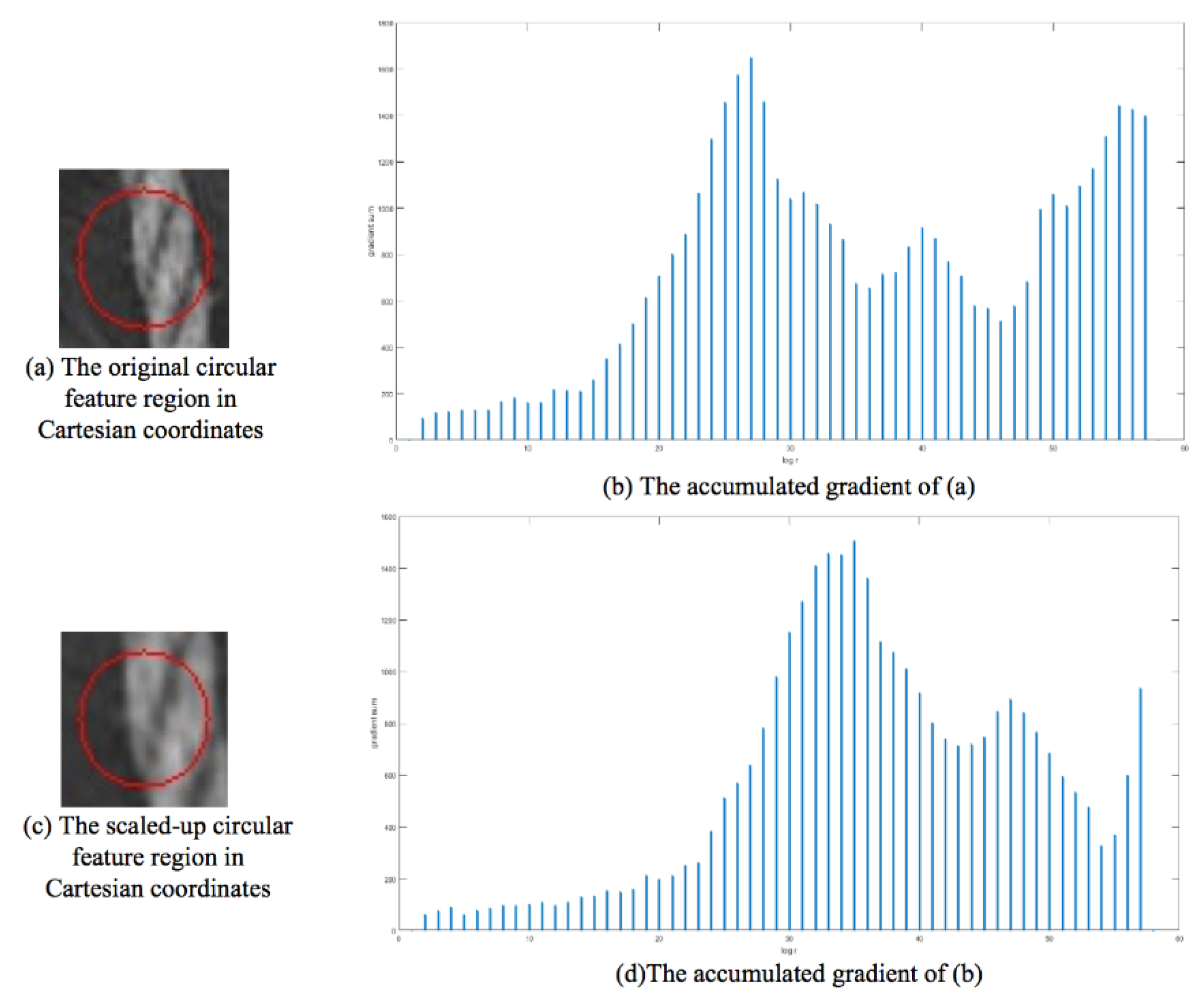
The proposed method uses the location of the maximum gradient along the radial direction to represent the scale of a feature region. The estimation of the scale representation of a feature region is shown in Figure 4. First, we transform the circular feature region in a 24-pixel radius into Log-polar coordinates using Equations (1) and (2). Second, we perform a one-dimensional gradient operation on the transformed Log-polar image to obtain the horizontal gradient along the log-radius (horizontal) axis. We sum the gradient values along the angular (vertical) axis for each log-radius to form a one-dimensional accumulated gradient with the radius as its index. We locate the maximum of the accumulated gradient and use its corresponding radius to represent the scale of the feature region. In other words, we use the radius of one of the concentric circles that has the largest accumulated radial gradient in the Cartesian coordinate system to represent the scale of the feature region.
Denote the feature region as f C ( x , y ) and its corresponding transformed image in the Log-polar coordinate system as f L ( ρ , θ ) . The one-dimensional gradient of the transformed image is calculated as:
g r a d ( ρ , θ ) = f L ( ρ + 1 , θ ) f L ( ρ 1 , θ ) .
The accumulated gradient for each log-radius (the blue curve shown in Figure 4) is
R ( ρ ) = θ g r a d ( ρ , θ ) = θ [ f L ( ρ + 1 , θ ) f L ( ρ 1 , θ ) ] .
The location of the maximum gradient of the accumulated gradient is
ρ m a x _ p o s = a r g m a x ρ R ( ρ ) = a r g m a x ρ θ [ f L ( ρ + 1 , θ ) f L ( ρ 1 , θ ) ] .
We represent the scale of the feature region by transferring the location of the maximum gradient into the Cartesian coordinate system, as shown in Equation (8),
s c a l e = t ρ m a x _ p o s ,
where t is the base of the Log-polar coordinate transformation defined in Equation (3).
Further investigation on the scaling and rotation transformation demonstrates the effectiveness of our method. We denote g C ( x , y ) as the scaled and rotated image of f C ( x , y ) , with scale factor a and rotation angle α degrees. The relationship between ( x , y ) and ( x , y ) is shown in Equations (9) and (10).
[ x y ] = [ a c o s α a s i n α a s i n α a c o s α ] [ x y ]
x = a x c o s α a y s i n α ,   y = a x s i n α + a y c o s α
Denote the corresponding image of g C ( x , y ) in the Log-polar coordinate system as g L ( ρ , θ ) , we have
ρ = 0.5 log t ( x 2 + y 2 ) = 0.5 log t [ ( a x c o s α a y s i n α ) 2 + ( a x s i n α + a y c o s α ) 2 ] .
According to Equation (2), we can obtain
ρ = 0.5 log t [ ( a t ρ c o s θ c o s α a t ρ s i n θ s i n α ) 2 + ( a t ρ c o s θ s i n α + a t ρ s i n θ c o s α ) 2 ] = 0.5 log t { [ a t ρ cos ( θ + α ) ] 2 + [ a t ρ sin ( θ + α ) ] 2 } = 0.5 log t ( a 2 t 2 ρ ) = log t a + ρ ,
θ = t a n 1 ( y x ) = t a n 1 ( a x s i n α + a y c o s α a x c o s α a y s i n α ) = t a n 1 ( t ρ c o s θ s i n α + t ρ s i n θ c o s α t ρ c o s θ c o s α t ρ s i n θ s i n α ) = θ + α .
Equation (12) shows that the scale change of a feature region in the Cartesian coordinate system leads to a shift along the radial axis in the Log-polar coordinate system. Equation (13) shows the rotation transformation in the Cartesian coordinate system corresponds to translation along the angular axis in the Log-polar coordinate system. For scaled and rotated image, we can estimate the location or the radius of the maximum accumulated gradient by Equation (14).
ρ m a x _ p o s = a r g m a x ρ θ [ g L ( ρ + 1 , θ ) g L ( ρ 1 , θ ) ] = a r g m a x ρ + log t a θ + α [ f L ( ρ + 1 , θ ) f L ( ρ 1 , θ ) ] = a r g m a x ρ θ [ f L ( ρ + 1 , θ ) f L ( ρ 1 , θ ) ] + log t a = ρ m a x _ p o s + log t a
And the detected scale representation for g C ( x , y ) is
s c a l e = t ρ m a x _ p o s = t ρ m a x _ p o s + log t a = t ρ m a x _ p o s · t log t a = a · s c a l e .
Equation (14) shows that, for a scaled and rotated feature region, the translation of the maximum accumulated gradient is proportional to the scale factor a . An example of the translation of the maximal accumulated gradient is shown in Figure 5. Figure 5a shows a feature region from an actual image. Figure 5c is the same region but enlarged by 1.5 times and cropped to have the same size as Figure 5a. The accumulated gradient of the original region and the enlarged region are plotted separately and shown in Figure 5b,d. The maximum gradient shifts to the right along the log t r axis because of the scale factor 1.5.
Equation (15) indicates that the scale factor between the two feature regions can be calculated as the ratio of their estimated scale representations. For example, the obtained scale representation of the original feature region is 3.79748 (Figure 5b), while the scale representation of the scaled feature region is 5.72002 (Figure 5d). The estimated scale factor of between the two feature regions is 1.50734, which is nearly the actual scale factor of 1.5. This simple experiment proves that the location of the maximum accumulated gradient can be used as a good representation of the scale of the feature region. All feature regions will be normalized to the same reference size before their SYBA descriptors can be calculated for matching. This scale normalization makes the SR-SYBA algorithm scale invariant.

3.3. Orientation Representation Estimation

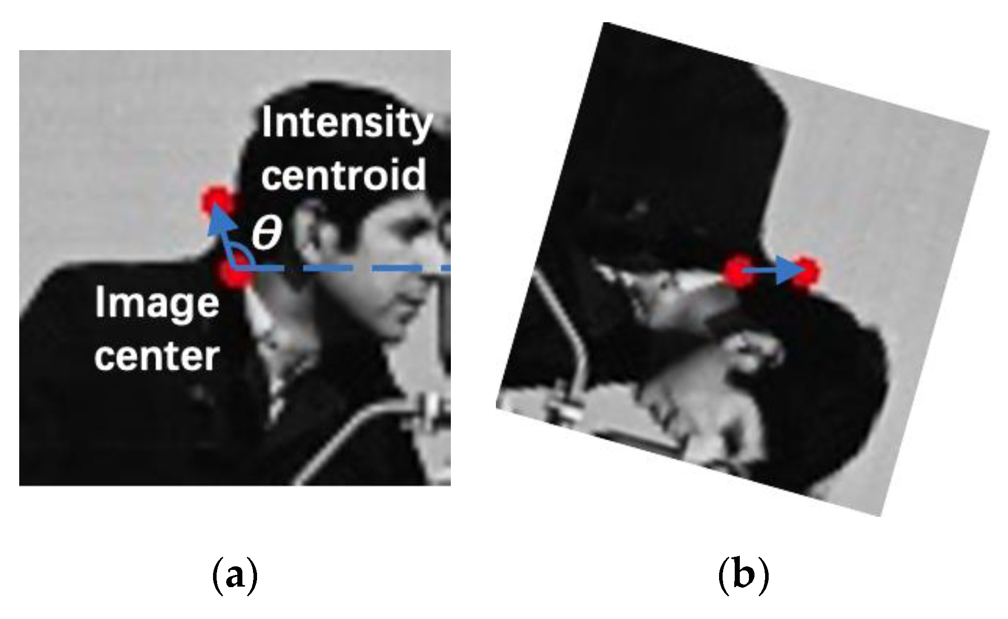
Study shows that the location of intensity centroid of an image also experiences corresponding conversion in image transforms due to scaling and rotation [22]. In other words, the length of the line connecting the center of the feature region and its intensity centroid increases proportionally to the increase of the scale, and its orientation rotates the same amount as the rotation of the image. With the detected scale of the feature region, we can determine what size of the feature region to calculate the intensity centroid and further represent the region’s orientation by calculating the orientation of the line connecting the feature region center and the intensity centroid. Assuming s is the estimated scale, we crop the feature region of the size of the multiples of s × s to calculate the intensity centroid. The intensity centroid is calculated using the moment of the neighborhood I ( x , y ) [23], as shown in Equations (16) and (17),
C = ( m 10 m 00 , m 01 m 00 )
m p q = x , y x p y q I ( x , y )
where ( x , y ) denotes the pixel of the feature region in the Cartesian coordinates, and m p q is the image moment of order ( p + q ) . The orientation representation of this feature region is calculated as the direction of the vector from the feature region center to the intensity centroid,
θ = arctan ( m 01 m 00 / m 10 m 00 ) = arctan ( m 01 / m 10 ) .
The SR-SYBA algorithm uses this angle to perform orientation normalization for the feature region to achieve rotation invariance. Figure 6 gives an illustration of this orientation representation estimation process. Figure 6a shows the representation of the orientation θ as the orientation of the vector from the center of the region to the intensity centroid. Figure 6b shows the orientation of the feature region after being normalized to θ = 0 degree.

3.4. Scale and Orientation Normalization

Using the estimated scale and orientation representations, all feature regions can be normalized to the same reference scale and orientation before matching. For example, suppose the reference scale is 15 and the reference orientation is 0°, given a feature region with a scale representation s and an orientation representation θ , the feature region is normalized using Equation (10) with scale factor a = 15 / s and rotation angle α = θ . The FRI (Feature Region of Interest) is then extracted in the normalized feature region for SYBA description. This pre-processing ensures the SR-SYBA to have image scale and rotation invariance. Figure 7 presents an example of scale and rotation normalization and FRI extraction.

3.5. SR-SYBA Algorithm

Compared to the original SYBA algorithm, our SR-SYBA algorithm only requires a little additional memory to store the feature region after Log-polar coordinate transformation for scale representation estimation. It obtains invariance to scaling and rotation transformations at the cost of storing an additional small image patch. Compared to the methods that determine the scale using image pyramid, our SR-SYBA algorithm is quite storage-efficient and applicable to embedded devices.
Figure 8 shows the flowchart of the SR-SYBA algorithm. The ORB (Oriented FAST and Rotated BRIEF) algorithm is used to detect feature points in the grayscale image. A small circular feature region surrounds each feature is transformed to the Log-polar coordinate system. The transformed image is then used to estimate its scale and orientation representations. The original rectangular feature region in the Cartesian coordinate system is resized to a reference scale and rotated to a reference orientation (horizontal) according to its scale and orientation representations. After the scale and orientation normalization, the SYBA algorithm is applied to the normalized feature region to calculate a feature descriptor for matching.

4. Experiments and Discussion

4.1. Verification of Scale Representation Estimation

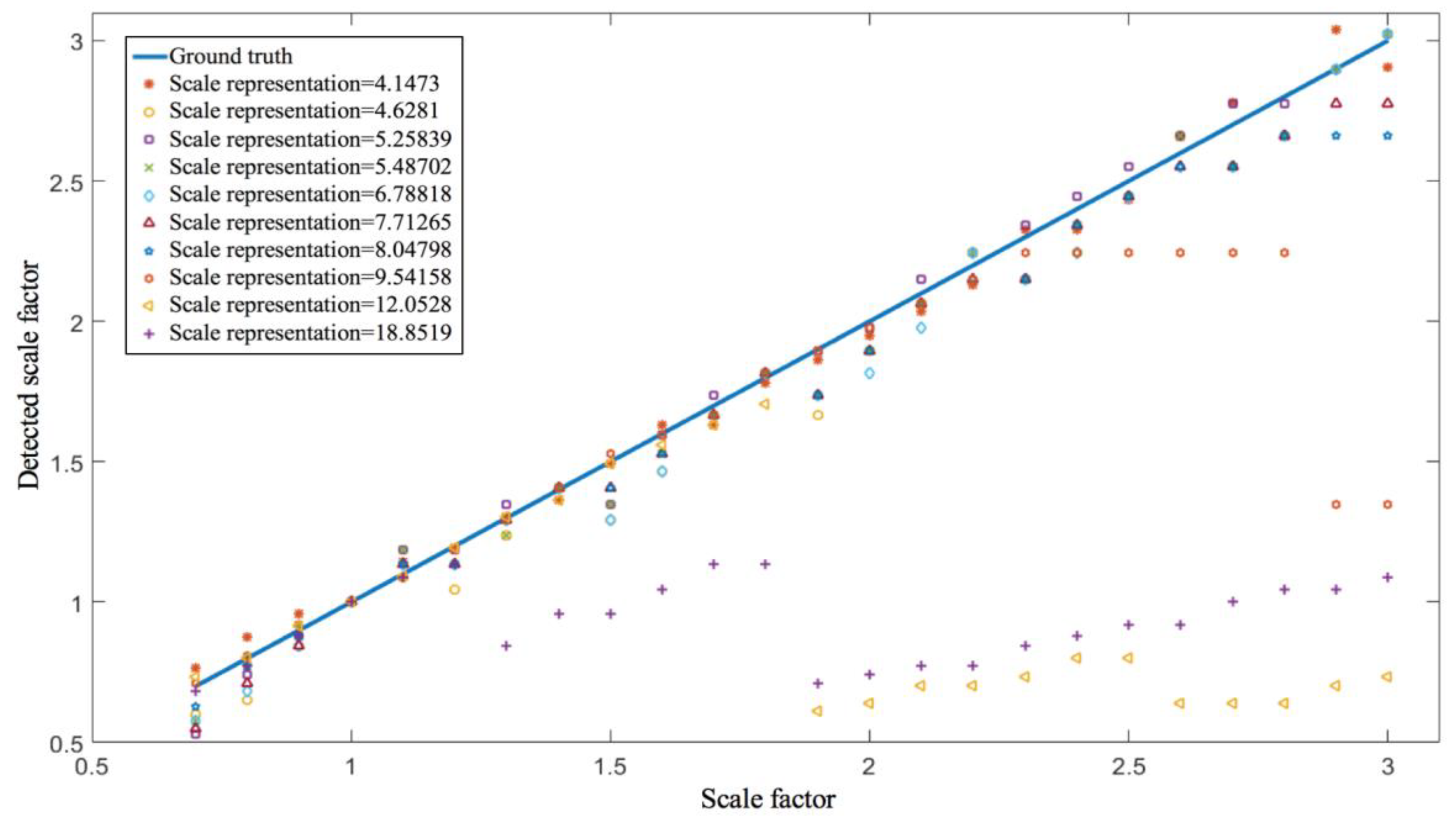
We performed this experiment with standard Lena image to demonstrate the effectiveness of the proposed scale representation estimation method. We detected 150 feature points of Lena using the ORB (Oriented FAST and Rotated BRIEF) algorithm. To verify the accuracy of our scale representation estimation, we calculated the scale representations of these 150 feature points and selected 10 that have distinct scale representations ranging from 4.14 to 18.85. We cropped a region of 35 × 35 and resized it by 0.7–3.0 at a 0.1 interval to generate 24 resized feature regions for each of these 10 feature points for experiment. The scale representations of these 240 resized regions were estimated using our method outlined in Section 3.2. The scale factor was calculated as the ratio of the scale representation of the original feature region to the scale representations of it corresponding 24 resized regions. The parameter r e was set to 24 in this experiment. We plotted the relationship between the calculated scale factors and the ground truth scale factors in Figure 9. The ground truth is on the y = x line, the solid line in Figure 9.
Figure 9 shows the effectiveness of our scale representation estimation algorithm as most of the points were very close to the ground truth. Some scale factors calculated for feature regions with a large-scale representation fell far from the ground truth. This was due to the fixed radius of 24 pixels, as scale representation estimation limited the allowable scale factor. The maximum allowable scale factor α is 24 / s for a feature region with a scale representation s. For example, for a large-scale representation s = 18.85, the largest allowable scale factor is 24/18.85 = 1.27. Our scale representation estimation algorithm failed when the scale factor exceeded its limit.
As shown in Figure 9, for the feature region with a scale representation of 8.048 (blue star), the last two scale factors (2.9 and 3.0) were very close to its allowable limit and were slightly off of the ground truth. For the feature region with a 9.54 scale representation (orange circle), the last six scale factors exceeded its detectable limit of 2.51 (24/9.54) and were not estimated corrected. Similarly, for scale representations 12.05 (yellow triangle) and 18.85 (purple cross), their respective allowable limit was 1.99 and 1.27. Only twelve yellow triangles (scale factors 0.7–1.8) and six purple crosses (scale factors 0.7–1.2) were estimated correctly. The larger the scale representation, the smaller the number of correct scale factors that can be estimated correctly.
Removing those scale factors that exceed their allowable limits, the scale representation estimation algorithm performed perfectly. Increasing the circular feature region radius will increase its allowable range. However, the larger the radius, the more likely the algorithm is to be affected by interferences, e.g., spurious local maxima and random noise. Based on our experiments, 24 was the most suitable radius for scale representation estimation and was chosen for all our experiments.

4.2. Performance Comparison with the Original SYBA

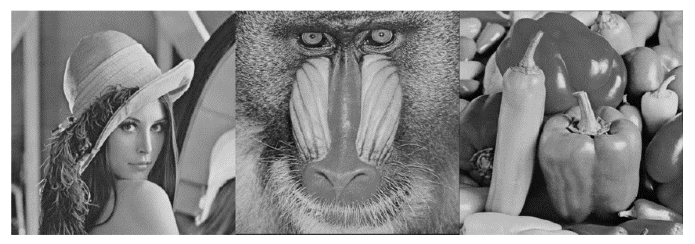
We compared SR-SYBA’s matching performance with the original SYBA under the same experimental settings to demonstrate its scale and rotation invariance. We selected three standard images that are commonly used for image processing: Lena, Baboon and Pepper, as shown in Figure 10.

4.2.1. Scaling Variation

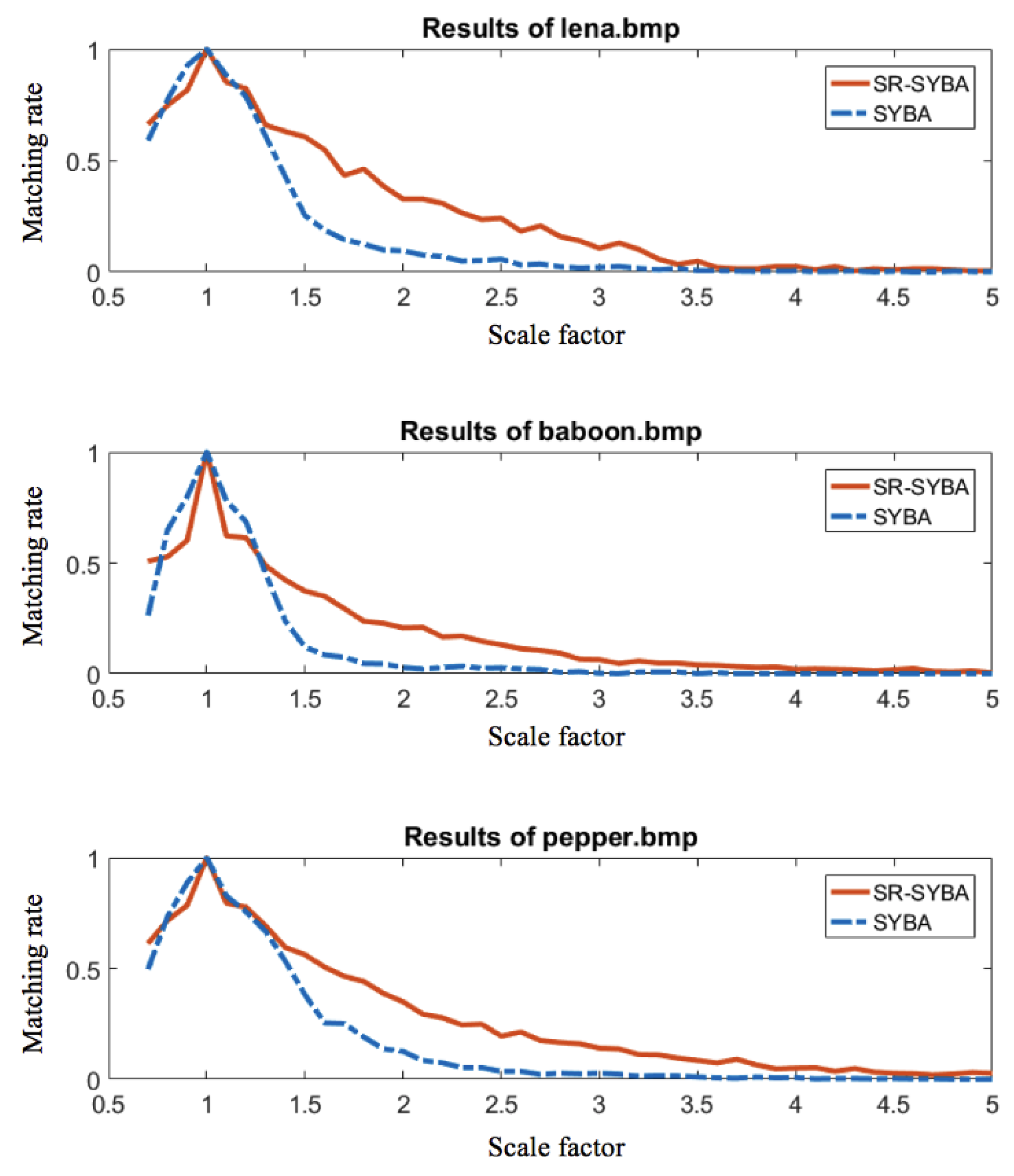
As for performance comparison under scaling variation, we first resized the image by 0.7–5.0 at a 0.1 interval, and tested the performance of these two algorithms for matching the resized image with the original. For a fair comparison, the same feature detector ORB was used for both SR-SYBA and SYBA. Brute Force matching [24] was performed for feature matching. Correct matches were filtered through the real affine matrix from which the error bound was set to 5 pixels. We define the matching rate as the ratio of the number of correct matches to the number of detected feature points. Suppose that the number of feature points detected for two matching pictures is N 1 , N 2 , and the number of correct matches founded is M . The matching rate R is defined as Equation (19),
R = M m i n ( N 1 , N 2 )
where m i n ( · ) takes the smaller one of the two values. The performance curves of SR-SYBA and SYBA under scaling variation corresponding to the three images are shown in Figure 11.
The overall performances of both algorithms declined with the increasing scale factor. This held truth for both the SR-SYBA and the SYBA algorithms, as shown in Figure 11. However, SR-SYBA showed significant performance improvement over the SYBA algorithm, manifested by the gap between the two curves of matching rate of the three charts in Figure 11. Overall, the experiment results showed that the SR-SYBA algorithm improved the matching performance of SYBA in terms of matching rate with scaling variations.

4.2.2. Rotation Variation

Experimental settings for rotation variation were similar to those for scaling variation. We rotated the three select images shown in Figure 10 by 10–350 degrees at a 10-degree interval and tested the performance of these two algorithms by matching features from the rotated image with features in the original image. Figure 12 shows the performance curves of SR-SYBA and SYBA under rotation variations for all three select images.
Figure 12 shows the matching rate of SR-SYBA with rotation variations was also superior to SYBA. SYBA’s performance exhibited a dramatic fall after the rotation angle became greater than 20 degrees, while SR-SYBA maintained the matching rate above 0.5 in all cases. We noticed that there was an interesting 90-degree cycle for SR-SYBA’s matching rate. The reason was that the pixels within the square region rotated by 90, 180, 270, and 360 degrees are the exact replicas of the original pixels without interpolation.

4.3. Performance Comparison with rSYBA

We compared the proposed SR-SYBA feature descriptor with our previous work of rSYBA following the same experiment settings in [18]. Experiments were conducted on the BYU Scaling and Rotation Dataset [18], which contains an original picture and its eight scaled and rotated versions. We matched the scaled and rotated images to the original image. Correct matches were filtered through the real affine matrix from which the error bound was set to 5 pixels. Matching rate was applied for evaluating the performance of rSYBA and SR-SYBA. The comparison results of rSYBA and SR-SYBA are shown in Table 1.
As shown in Table 1, rSYBA had higher matching rates than SR-SYBA in the case that scale factor is 0.9 and 1.05. SR-SYBA performed better when the scale difference between the two images increased. Specifically, rSYBA was limited to scale factors between 0.8 and 1.2. SR-SYBA’s performance also surpassed rSYBA for all rotation angles. Overall, SR-SYBA achieved better performance than rSYBA on the BYU Scaling and Rotation Dataset for large scale factors and rotation angles.
We compared the processing time of these two methods using the same parameters above. This experiment was carried out using a computer system equipped with an Intel i5-8400 [email protected] GHz and 8 GB RAM running 64-Bit Windows 10 operating system. The whole feature description and matching process can be divided into three steps: scale invariance, rotation invariance, and SYBA calculation and matching. SR-SYBA achieves scale invariance by calculating the scale representation and then normalizing the FRI to the reference scale, whereas rSYBA rescales the FRI into multiple sizes for matching. The number of sizes depends on the desired scaling range and scaling accuracy. Both methods achieve rotation invariance in one shot by calculating the FRI’s dominant orientation and rotate it once to a reference orientation. rSYBA requires more time for SYBA calculation and matching than SR-SYBA because it has to process more FRI’s.
Table 2 shows the processing time for each step between the two methods. We started with 300 features but 5 scales for rSYBA. SR-SYBA took 6.57 milliseconds to calculate one FRI’s scale representation and rescale it to the reference scale, whereas rSYBA took only 0.78 milliseconds to rescale one FRI to five different scales. SR-SYBA was much more efficient (0.012 millisecond per FRI) in providing rotation invariance than rSYBA (6.24 milliseconds per FRI). For SYBA calculation and matching, rSYBA took 9.33 milliseconds to compute the SYBA descriptor for 300 FRI’s and perform brute force matching 300 × 300 times, whereas rSYBA took 5 times as long to calculate the SYBA descriptor for 1500 FRI’s and perform matching 300 × 1500 times. rSYBA took nearly 5 times longer than SR-SYBA. Note that in Table 2, the rotation invariance for rSYBA was performed after rescaling. Even if calculating the dominant orientation for each FRI before rescaling, all 1500 FRI’s would still need to be rotated to the reference orientation. More than five scales would be needed to increase the scaling variation range and scaling invariance accuracy, which would slow rSYBA even further.

4.4. Performance Comparison with Other Feature Fescription Algorithms

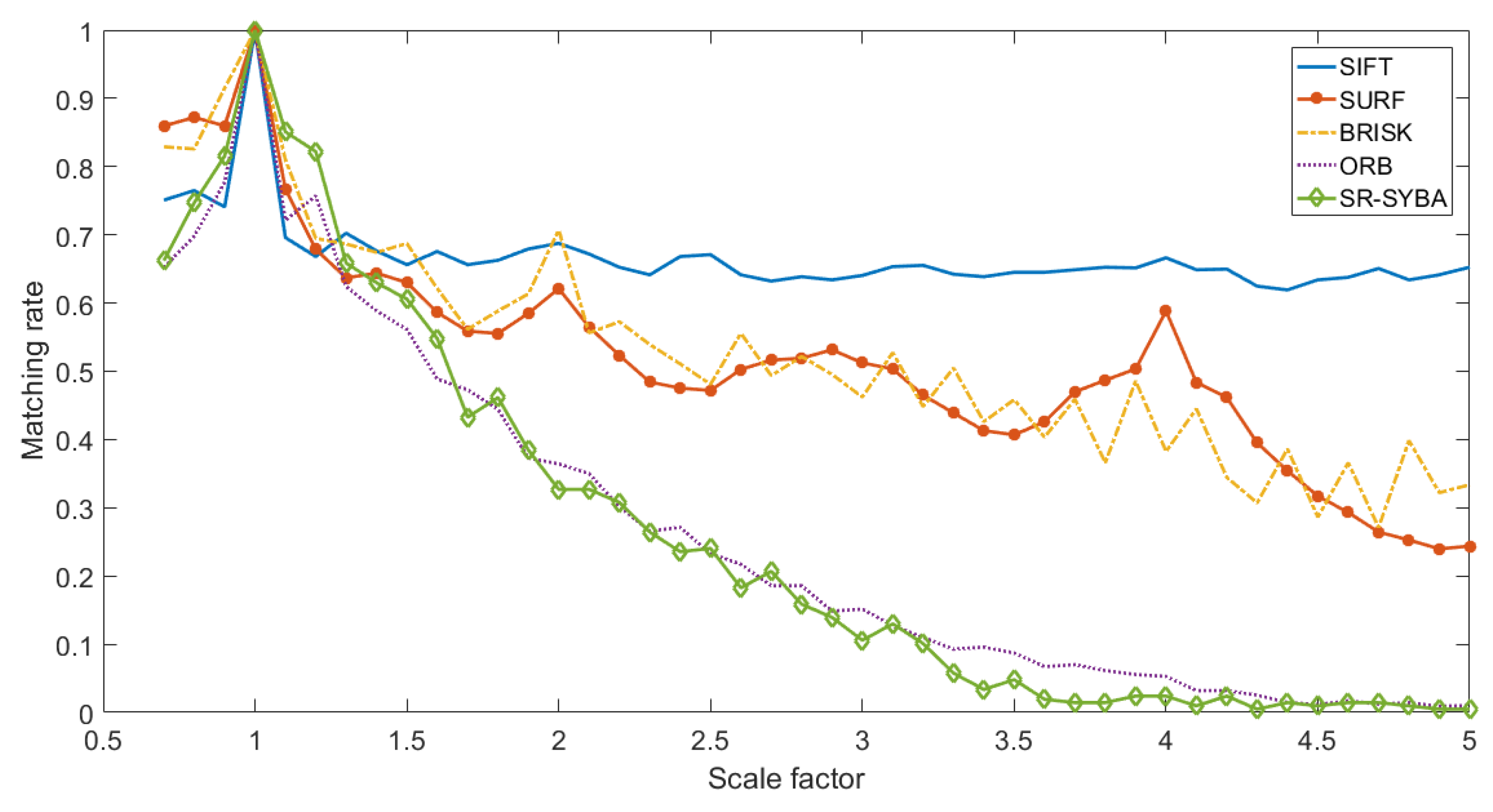
We compared our SR-SYBA feature descriptor with other feature description algorithms in the cases of scaling and rotation variations. The experiment settings were similar to the ones in Section 4.2. Lena was used for these experiments. We tested the matching performance of each algorithm after the image was resized by 0.7–5.0 at a 0.1 interval. Similarly, Brute Force matching and matching rate were applied. ORB feature detection was again used for SR-SYBA feature detection. SIFT, SURF, BRISK, ORB, and SR-SYBA were included in this comparison. The original SYBA and the improved rSYBA were not included in this experiment because the comparisons in Section 4.2 and Section 4.3 already demonstrated SR-SYBA’s superior performance. The experimental results are shown in Figure 13.
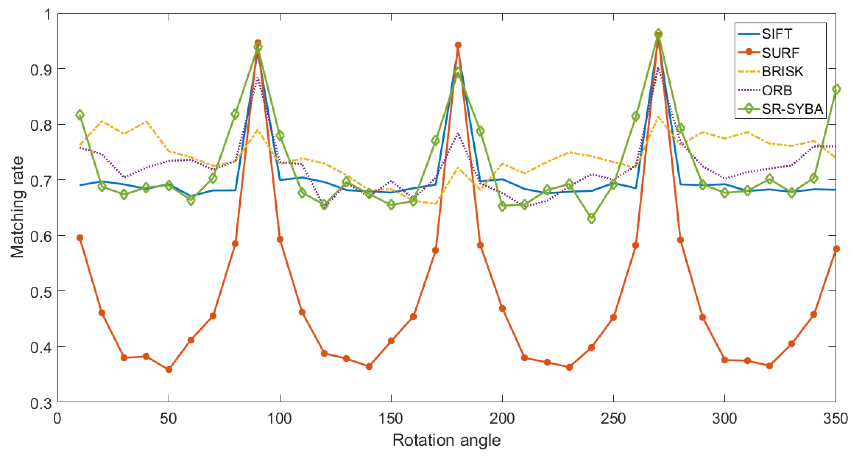
As shown in Figure 13, SIFT, SURF and BRISK performed better under such experimental settings. The performances of SR-SYBA and ORB were close, while SR-SYBA was better for smaller scale factors and ORB was better for larger scale factors. Similar test for rotation variation was also performed for these algorithms. The Lena image was rotated by 10–350 degrees at a 10-degree interval. Figure 14 shows that most feature description algorithms provide rotation invariance. SR-SYBA provided the best rotation invariance. Its matching rate curve reached the highest peak and dropped slower than other algorithms when rotation angle moved away from 90, 180, 270, and 360 degrees.

4.5. Memory Usage Comparison with Other Feature Description Algorithms

We also measured the memory usage for feature detection and description for each algorithm. The test was performed with varying image sizes, ranging from 397 × 298 to 3968 × 2976, in order to evaluate how memory usage changes as the image size increases. The memory usage for each algorithm was monitored using the debugging tools of Visual Studio 2017. All algorithms were tested on the same system. To eliminate the bias from different number of feature points, all algorithms were set to detect and describe 500 feature points. Considering ORB needs to construct image-pyramid for feature point detection, SR-SYBA algorithm collocates with FAST [25] feature detection algorithm. Table 3 shows that our SR-SYBA algorithm required much less space than other classical feature description algorithms. SR-SYBA only required 0.1MB more memory than SYBA, while achieving much better scale and rotation invariance. Table 3 also presents that as the image size increased, the memory usage for each algorithm also increased. The memory usage for other algorithms was around 4 to 1000 times that of SR-SYBA, and the gap of memory usage between SR-SYBA and other algorithms increased with the increasing image size. Although ORB and SR-SYBA had similar performance in the experiments shown in Section 4.3, SR-SYBA utilized less than a quarter of ORB’s memory space. This experiment demonstrated that SR-SYBA is more suitable for applications using embedded systems where memory resources are scarce.

4.6. Performance for Real Sscenes

In the previous section, we compared different feature-based image matching algorithms by matching the original image to its own scaled and rotated version. In this section, we conducted the same experiments but with the images from real scenes that have real scaling and rotation changes not through interpolation.

4.6.1. The Oxford Affine Dataset

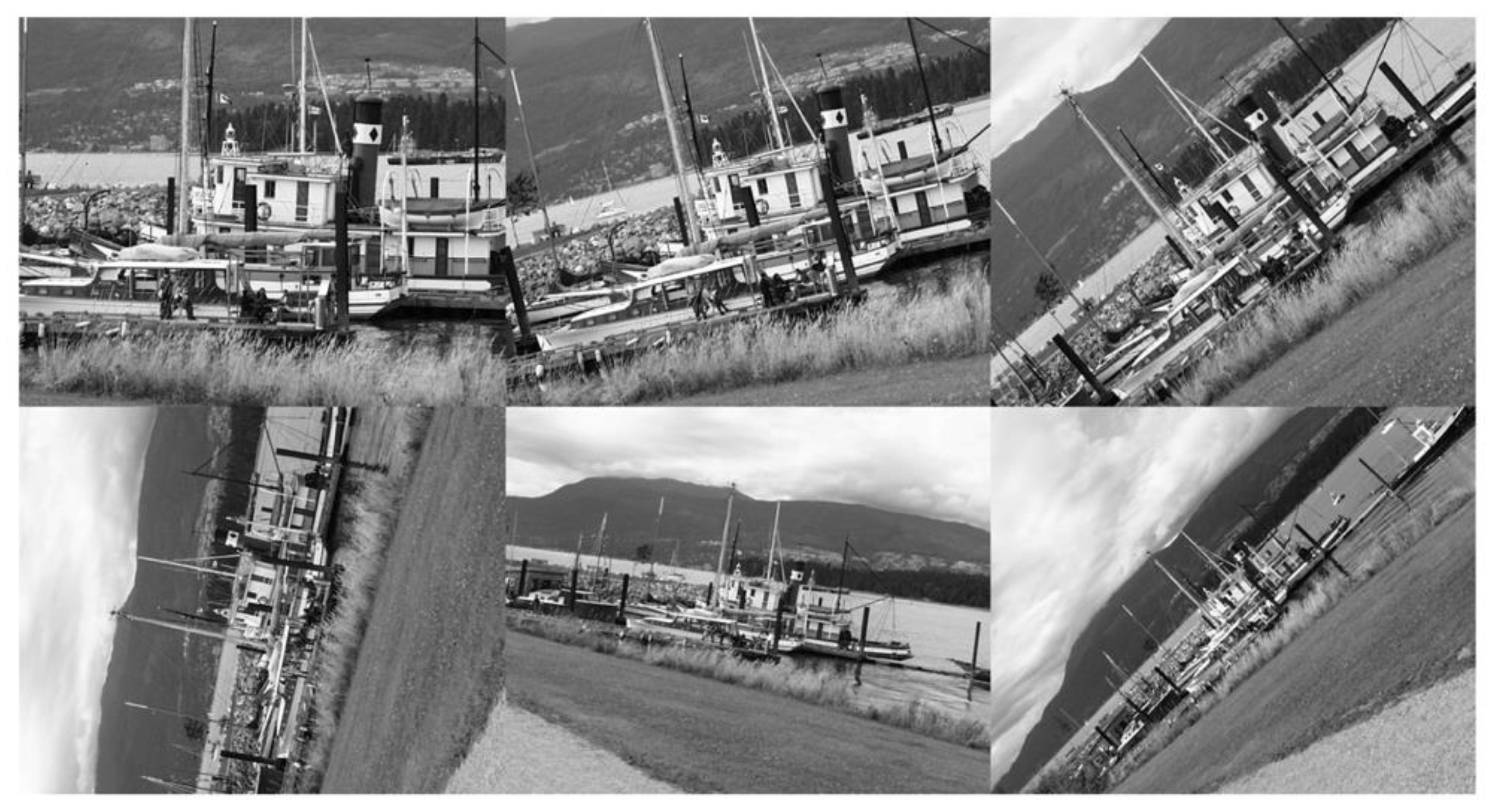
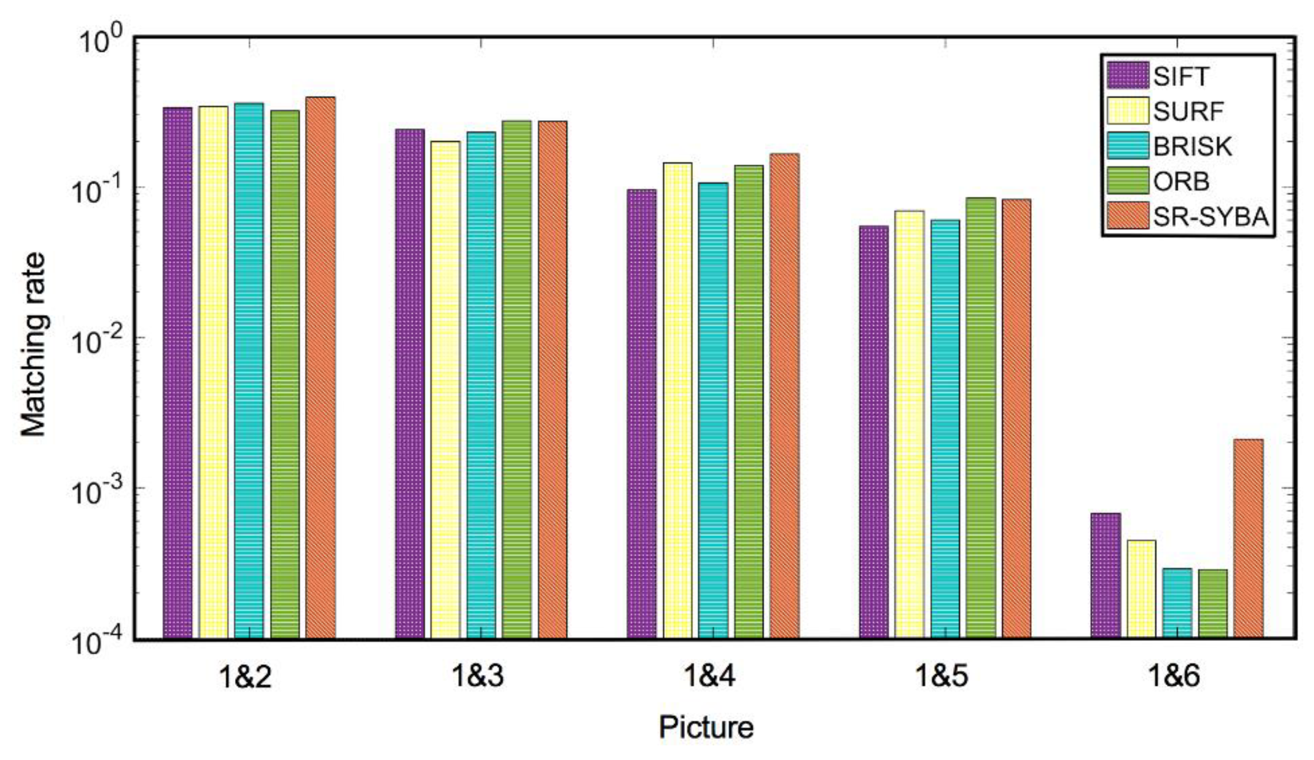
We used the boat image sequence from Oxford Affine dataset [26] for evaluation. This image sequence has six images of the same scene with increasing shooting distance and angle, as shown in Figure 15. The first image was used as the reference image, and the other five images were matched to the reference image individually. The correct matching points were filtered through the affine matrix provided by the dataset. We used the same matching rate defined in Section 4.2 as the criteria for evaluation. The results obtained by SIFT, SURF, BRISK, ORB, and SR-SYBA algorithms respectively are plotted in histograms in Figure 16. The vertical axis (matching rate) was scaled to logarithmic for ease of comparison.
As shown in Figure 16, SR-SYBA obtained the best overall performance, maintaining the best or second-best matching rate for all image pairs. The matching performance of all five algorithms was quite comparable for the first four pairs. For the last pair, SR-SYBA’s performance surpassed all other algorithms by almost an order of magnitude.

4.6.2. Statistical t-Test Using the BYU Feature Matching Dataset

We used the BYU Feature Matching dataset [10] to perform a more thorough statistical t-test to further compare SIFT, SURF, BRISK, ORB, and SR-SYBA. This dataset was created specifically for the statistical t-test [10]. Similar to the Oxford Graffiti dataset, it includes six images in each image sequence with increasing image perturbations. The first image was used as the reference image, and the other five images were matched to the reference image individually. It has 20 sets of these image sequences for each image perturbation instead of just one in the Oxford dataset. With 20 times the amount of data, we were able to perform a meaningful statistical t-test. Experiments were conducted in a similar manner as those in Section 4.6.1 and Section 4.6.2.
ORB was again used for feature detection. We detected 6000 features from each image for matching. The ground truth perspective transformation was calculated from four manually selected matching feature pairs. The distance between the matched feature point and the ground truth must be no greater than 5 pixels to be considered a correct match. Table 4 shows the average matching rates of all methods and the p-values between SR-SYBA and other methods. SR-SYBA had the highest average matching rate of all methods. The p-values from Image pair 1|3 for SURF and BRISK were larger than 0.05, which indicated the image pair failed to provide a statistically meaningful comparison between SR-SYBA and the other two methods. All other p-values were significantly smaller than 0.05 and most of them were much smaller than 0.01.

5. Application for Vision-Based Measurement

Vision-based measurement refers to the measurement of the size or distance of an object based on the picture taken by a camera [27]. In most cases, vision-based measurement requires a known object as the reference, and image matching is required to locate the position and size of the reference object. We tested our SR-SYBA algorithm for this real-world application.
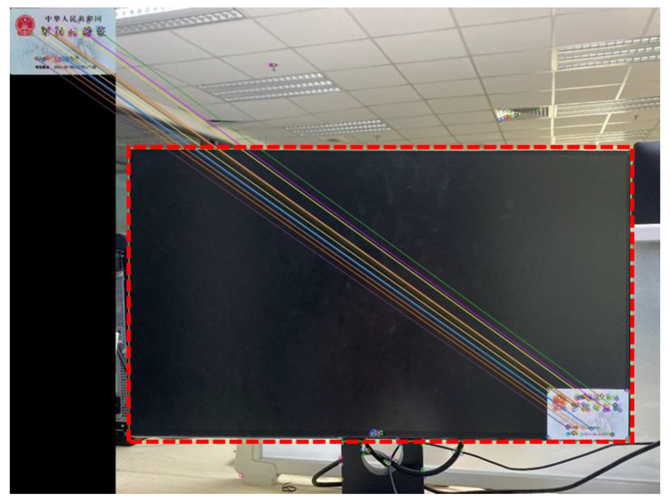
One good example of this vision-based measurement application is an online shopping App for mobile devices. The App provides a function for rough measurement of an object using phone camera [28]. Suppose a customer wanted to order a suitable cover for his computer monitor. The customer would be asked to take a picture of the monitor together with a known reference object, e.g., an ID card. Then the customer would need to frame his monitor to be measured. The App will report the estimated height and width. This helps the customer get the recommended size of the product. This function requires image matching. We demonstrated the whole process with our SR-SYBA algorithm.
First, we took a picture of the reference object, i.e., the ID card, and measured its actual height and width. Then, we took another picture containing both the reference object and the object to be measured and framed the object to be measured. Next, the SR-SYBA algorithm was used to match the two images to obtain an affine matrix fitted by the RANSAC [29] algorithm. With the affine matrix, the reference image can be mapped to the measuring image [30]. Assuming the point before and after the mapping is ( x , y ) and ( x 1 , y 1 ) , respectively, the mapping relation with a 2 × 3 affine matrix H is in Equation (20).
[ x 1 y 1 ] = H · [ x y 1 ] = [ h 00 h 01 h 02 h 10 h 11 h 1 ] · [ x y 1 ] = [ h 00 x + h 01 y + h 02 h 10 x + h 11 y + h 12 ]
Thus, based on the ratio of occupied pixels for the mapped reference and the object to be measured, together with the actual size of the reference object, the actual size of the object can be estimated.
Six objects with different aspect ratio are chosen for measurement and the results are recorded in Table 5. An example image matching result with SR-SYBA algorithm is shown in Figure 17, where the dashed rectangle is the frame of the object to be measured.
Table 5 shows that all error rates of SR-SYBA algorithm for this vision-based measurement task were less than 3%, whether the object was much larger than or similar to the reference object. Considering the existence of the manually framing error and the camera distortion, such accurate results confirm the effectiveness of the SR-SYBA algorithm for practical applications. This vision-based measurement technique can be applied to either object measurement estimation in daily life [30] or industrial instrumentation [31].

6. Conclusions

This paper proposes an algorithm called SR-SYBA to solve the scale and rotation invariance problem for the SYBA feature description algorithm. The main advantage of the SR-SYBA algorithm is its small memory usage, which is critical for resource-limited devices. SR-SYBA adds scale and orientation normalization as pre-processing before using SYBA for description and matching. The scale representation is determined by converting the feature region to Log-polar coordinates to ensure the high stability required for scale representation estimation. The orientation of the feature region is determined by the orientation of the vector connecting the feature region center to the intensity centroid in Cartesian coordinates. The proposed SR-SYBA algorithm is a scale-invariant and rotation-invariant feature description algorithm with computational simplicity and small memory usage.
Experiment results show that the SR-SYBA algorithm successfully addresses the original SYBA’s shortcomings for image matching applications with scaling and rotation variations, and significantly boosts its matching accuracy. The SR-SYBA algorithm was compared with other commonly used feature description algorithms: SIFT, SURF, BRISK, and ORB. Experimental results show that the SR-SYBA algorithm achieved comparable or better performance than ORB, while only using less than a quarter of its memory usage. Besides, SR-SYBA gave the best matching results for images from real scenes. Finally, this paper demonstrates the feasibility of the SR-SYBA algorithm for a practical application of vision-based measurement.

Author Contributions

Conceptualization, M.Y. and D.Z.; methodology, M.Y.; software, M.Y. and A.D.; validation, M.Y. and D.Z.; formal analysis, M.Y.; investigation, M.Y., D.Z. and D.-J.L.; resources, M.Y. and D.Z.; data curation, M.Y.; writing—original draft preparation, M.Y.; writing—review and editing, D.Z. and D.-J.L.; visualization, M.Y.; supervision, D.Z.; project administration, D.Z.; funding acquisition, D.Z. All authors have read and agreed to the published version of the manuscript.

Funding

This research was supported by Guangzhou Municipal People’s Livelihood Science and Technology Plan (201903010040), the Science and Technology Planning Project of Guangdong Province of China (2019B070702004), and Science and Technology Program of Guangzhou, China (202007030011).

Conflicts of Interest

The authors declare no conflict of interest. The funders had no role in the design of the study; in the collection, analyses, or interpretation of data; in the writing of the manuscript, or in the decision to publish the results.

References

  1. Krishnan, R.; Anil, A.R. A survey on image matching methods. Int. J. Latest Res. Eng. Technol. 2016, 22, 58–61. [Google Scholar]
  2. Yao, J. Image registration based on both feature and intensity matching. In Proceedings of the 26th IEEE International Conference on Acoustics, Speech, and Signal Processing, Salt Lake City, UT, USA, 7–11 May 2001; pp. 1693–1696. [Google Scholar]
  3. Hassaballah, M.; Abdelmgeid, A.A.; Alshazly, H.A. Image Feature Detection and Descriptor, 1st ed.; Springer: Heidelberg, Germany, 2016; pp. 11–45. [Google Scholar]
  4. Lowe, D.G. Distinctive image features from scale-invariant keypoints. Int. J. Comput. Vis. 2004, 60, 91–110. [Google Scholar] [CrossRef]
  5. Bay, H.; Tuytelaars, T.; Van Gool, L. SURF: Speeded up robust features. In Proceedings of the 7th European Conference on Computer Vision, Graz, Austria, 7–13 May 2006; pp. 404–417. [Google Scholar]
  6. Calonder, M.; Lepetit, V.; Strecha, C.; Fua, P. BRIEF: Binary robust independent elementary features. In Proceedings of the 11th European Conference on Computer Vision, Heraklion, Greece, 5–11 September 2010; pp. 778–792. [Google Scholar]
  7. Leutenegger, S.; Chli, M.; Siegwart, R. BRISK: Binary robust invariant scalable keypoints. In Proceedings of the 2011 International Conference on Computer Vision, Barcelona, Spain, 6–13 November 2011; pp. 2548–2555. [Google Scholar]
  8. Rublee, E.; Rabaud, V.; Konolige, K.; Bradski, G. ORB: An efficient alternative to SIFT or SURF. In Proceedings of the 2011 International Conference on Computer Vision, Barcelona, Spain, 6–13 November 2011; pp. 2564–2571. [Google Scholar]
  9. Theodoros, G.; Yu, L.; Wei, C.; Micheal, L. A survey of traditional and deep learning-based feature descriptors for high dimensional data in computer vision. Int. J. Multimed. Info. Retr. 2019, 1–36. Available online: https://doi.org/10.1007/s13735-019-00183-w (accessed on 22 November 2019).
  10. Desai, A.; Lee, D.J.; Ventura, D. An efficient feature descriptor based on synthetic basis functions and uniqueness matching strategy. Comput. Vis. Image Underst. 2016, 142, 37–49. [Google Scholar] [CrossRef]
  11. Moravec, H.P. Obstacle Avoidance and Navigation in the Real World by a Seeing Robot Rover; Technical Report; Stanford University: Stanford, CA, USA, 1980. [Google Scholar]
  12. Harris, C.; Stephens, M. A combined corner and edge detector. In Proceedings of the Alvey Vision Conference, Manchester, UK, 31 August–2 September 1988; pp. 147–151. [Google Scholar]
  13. Ke, Y.; Sukthankar, R. PCA-SIFT: A more distinctive representation for local image descriptors. In Proceedings of the 2004 IEEE Computer Society Conference on Computer Vision and Pattern Recognition, Washington, DC, USA, 27 June–2 July 2004; p. ii. [Google Scholar]
  14. Kwang, M.Y.; Eduard, T.; Vincent, L.; Pascal, F. LIFT: Learned invariant feature transform. In Proceedings of the 14th European Conference on Computer Vision, Amsterdam, Netherlands, 8–16 October 2016; pp. 467–483. [Google Scholar]
  15. Daniel, D.; Tomasz, M.; Andrew, R. SuperPoint: Self-supervised Interest Point Detection and Description. In Proceedings of the 2018 IEEE/CVF Conference on Computer Vision and Pattern Recognition Workshops, Salt Lake City, UT, USA, 17 December 2018; pp. 337–349. [Google Scholar]
  16. Ono, Y.; Eduard, T.; Pascal, F.; Kwang, M.Y. LF-Net: Learning local features from images. In Proceedings of the 32nd Neural Information Processing System, Montreal, QC, Canada, 3–8 December 2018; pp. 1–11. [Google Scholar]
  17. Zhen, Z.; Wee, S.L. Deep graphical feature learning for the feature matching problem. In Proceedings of the 2019 International Conference on Computer Vision, Seoul, Korea, 27 October–2 November 2019; pp. 5087–5096. [Google Scholar]
  18. Zhang, D.; Raven, L.A.; Lee, D.J.; Meng, Y.; Desai, A. Hardware friendly robust synthetic basis feature descriptor. Electronics. 2019, 8, 847. [Google Scholar] [CrossRef] [Green Version]
  19. Matungka, R. Studies on Log-Polar Transform for Image Registration and Improvements Using Adaptive Sampling and Logarithmic Spiral. Ph.D. Thesis, Ohio State University, Columbus, OH, USA, 2016. [Google Scholar]
  20. Araujo, H.; Dias, J.M. An introduction to the log-polar mapping. In Proceedings of the II Workshop on Cybernetic Vision, Sao Carlos, Brazil, 9–11 December 1996; pp. 139–144. [Google Scholar]
  21. Tao, T.; Zhang, Y. Detection and description of scale-invariant keypoints in log-polar space. J. Image Graph. 2015, 20, 1639–1651. [Google Scholar]
  22. Schneider, P.J.; Eberly, D.H. Geometric Tools for Computer Graphics, 1st ed.; Morgan Kaufmann: Burlington, MA, USA, 2002; pp. 98–103. [Google Scholar]
  23. Rosin, P.L. Measuring corner properties. Comput. Vis. Image Underst. 1999, 73, 291–307. [Google Scholar] [CrossRef] [Green Version]
  24. Noble, F.K. Comparison of OpenCV’s feature detectors and feature matchers. In Proceedings of the 23rd International Conference on Mechatronics and Machine Vision in Practice, Nanjing, China, 28–30 November 2016; pp. 1–6. [Google Scholar]
  25. Trajković, M.; Hedley, M. Fast corner detection. Image Vision Comput. 1998, 16, 75–87. [Google Scholar] [CrossRef]
  26. Affine Covariant Features. Available online: http://www.robots.ox.ac.uk/~{}vgg/research/affine/ (accessed on 22 March 2020).
  27. Shirmohammadi, S.; Ferrero, A. Camera as the instrument: The rising trend of vision based measurement. IEEE Instrum. Meas. Mag. 2014, 17, 41–47. [Google Scholar] [CrossRef]
  28. What You See and Think—Requirements and Scenarios. Available online: www.muflyguo.com/archives/1557 (accessed on 22 March 2020).
  29. Fischler, M.A.; Bolles, R.C. Random sample consensus: A paradigm for model fitting with applications to image analysis and automated cartography. Commun. ACM 1981, 24, 381–395. [Google Scholar] [CrossRef]
  30. Brown, L.G. A survey of image registration techniques. ACM Comput. Surv. 1992, 24, 325–376. [Google Scholar] [CrossRef]
  31. Santos, E.S.F.; Xavier, W.B.; Rodrigues, R.N.; Botelho, S.S.C.; Werhli, A.V. Vision based measurement applied to industrial instrumentation. In Proceedings of the 20th World Congress of the International Federation of Automatic Control, Toulouse, France, 9–14 July 2017; pp. 788–793. [Google Scholar]
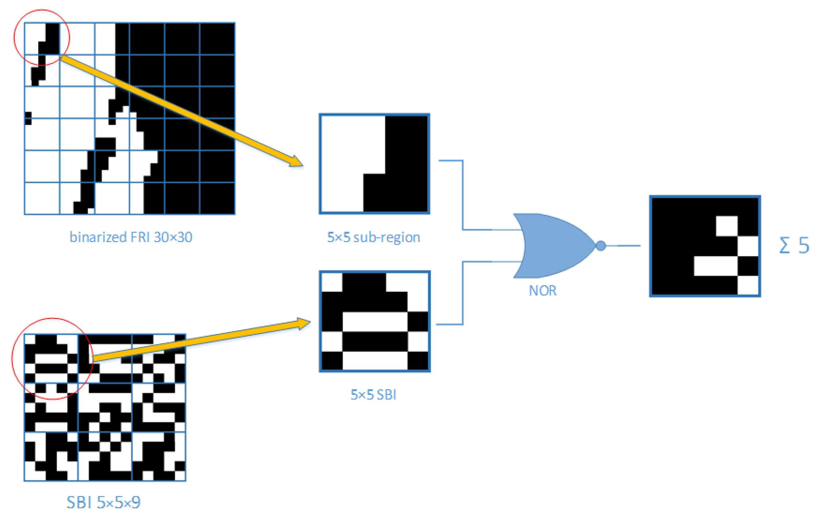
Figure 1. SYBA descriptor formation.
Electronics 09 00810 g001
Figure 2. SR-SYBA block diagram.
Electronics 09 00810 g002
Figure 3. An example of Log-polar coordinate transformation. (a) a circular feature region of a 24-pixel radius in the Cartesian coordinate system (the area in the dotted circle). (b) transformed rectangular block (74 × 150 pixels) in the Log-polar coordinate system.
Electronics 09 00810 g003
Figure 4. Scale representation estimation of a circular feature region.
Electronics 09 00810 g004
Figure 5. The accumulated gradients for the original and enlarged feature regions.
Electronics 09 00810 g005
Figure 6. (a) Orientation representation estimation with intensity centroid and (b) orientation normalization to horizontal.
Electronics 09 00810 g006
Figure 7. An example of scale and rotation normalization. (a) is the original feature region (70 × 70 pixels), with a scale representation of 16.6 and orientation representation of 45°. The normalized feature region based on the estimated scale and orientation representations is shown in (b). (c) is the FRI of 30 × 30 pixels extracted from the normalized feature region for SYBA description.
Electronics 09 00810 g007
Figure 8. Flowchart of the SR-SYBA algorithm.
Electronics 09 00810 g008
Figure 9. Scale factor calculation verification.
Electronics 09 00810 g009
Figure 10. Three images (from left to right: Lena, Baboon, and Pepper) used for comparison between the SR-SYBA and the original SYBA algorithms.
Electronics 09 00810 g010
Figure 11. Matching rate comparison between SR-SYBA and SYBA with scaling variations.
Electronics 09 00810 g011
Figure 12. Matching rate comparison between SR-SYBA and SYBA with rotation variations.
Electronics 09 00810 g012
Figure 13. Comparison with scaling variations.
Electronics 09 00810 g013
Figure 14. Comparison with rotation variations.
Electronics 09 00810 g014
Figure 15. The boat image sequence in the Oxford Affine dataset.
Electronics 09 00810 g015
Figure 16. Matching rate comparison with the Boat image sequence.
Electronics 09 00810 g016
Figure 17. An example of the matching result for a vision-based measurement task.
Electronics 09 00810 g017
Table 1. Matching rate comparison between rSYBA and SR-SYBA.
Image TransformationFeature CountMatching Rate (%)
rSYBASR-SYBA
Scale factor = 0.830055.3357.64
Scale factor = 0.930070.3369.67
Scale factor = 1.0530079.0075.67
Scale factor = 1.130073.6774.67
Scale factor = 1.230067.0072.33
Rotation degree = 530063.3378.33
Rotation degree = 730046.3375.67
Rotation degree = 1030054.0070.00
Rotation degree = 1530045.6756.67
Table 2. Processing time comparison between rSYBA and SR-SYBA (in milliseconds).
Scaling InvarianceRotation InvarianceSYBA & MatchingTotal
SR-SYBA300 × 6.57 = 1971300 × 0.012 = 3.69.33 for 300 × 3001983.93
rSYBA300 × 0.78 = 2341500 × 6.24 = 936046.65 for 1500 × 3009640.65
Table 3. The memory usage (MB) of each algorithm at runtime.
Image SizeSIFTSURFBRISKORBSR-SYBASYBA
397 × 29834.028.252.527.47.67.5
794 × 595114.052.156.428.87.97.8
1587 × 1190443.1130.461.236.09.49.3
2381 × 1786965.6262.872.048.211.611.5
3174 × 23811.7 × 103446.487.163.514.714.6
3968 × 29762.6 × 103682.5106.883.218.718.6
Table 4. Average matching rate and the p-values between SR-SYBA and other methods.
Image PairDataSIFTSURFBRISKORBSR-SYBA
1|2Average Matching Rate %31.0142.1745.8030.1452.58
p-value6.75 × 10−87.91 × 10−50.00831.25 × 10−8/
1|3Average Matching Rate %25.9638.1338.8225.6639.27
p-value4.77 × 10−40.38220.46020.0021/
1|4Average Matching Rate %19.1728.9728.6418.1733.83
p-value1.25 × 10−40.03680.02032.27 × 10−5/
1|5Average Matching Rate %18.9629.8428.1817.9636.17
p-value3.14 × 10−50.00127.16 × 10−42.28 × 10⁻⁶/
1|6Average Matching Rate %16.1325.8826.2815.0231.18
p-value1.35 × 10−40.01300.02663.29 × 10−5/
Table 5. The vision-based measurement results with SR-SYBA.
Object Actual Size (mm)Measurement Result (mm)Error (%)
Student card Length8584.2230.914
Width54.553.9720.969
Packing boxLength105103.6211.313
Width105106.4661.396
BookmarkerLength144145.0300.715
Width4039.9580.105
Book Length210206.4261.702
Width235229.3282.414
A4 paper Length210215.5412.639
Width297298.3140.442
Computer monitorLength537.6552.4502.762
Width314.3311.9460.749