Abstract
Ophthalmology is a core medical field that is of interest to many. Retinal examination is a commonly performed diagnostic procedure that can be used to inspect the interior of the eye and screen for any pathological symptoms. Although various types of eye examinations exist, there are many cases where it is difficult to identify the retinal condition of the patient accurately because the test image resolution is very low because of the utilization of simple methods. In this paper, we propose an image synthetic approach that reconstructs the vessel image based on past retinal image data using the multilayer perceptron concept with artificial neural networks. The approach proposed in this study can convert vessel images to vessel-centered images with clearer identification, even for low-resolution retinal images. To verify the proposed approach, we determined whether high-resolution vessel images could be extracted from low-resolution images through a statistical analysis using high- and low-resolution images extracted from the same patient.
1. Introduction
As the population ages, ophthalmology has become a core medical field. Ophthalmology not only treats severe diseases such as glaucoma but also non-disease issues such as vision correction. Minor diseases such as conjunctivitis can be diagnosed visually or through simple examinations; however, severe diseases that may lead to vision loss cannot be diagnosed accurately without a detailed examination performed by a physician.
An example of an ophthalmology examination is the retinal or fundus examination, in which a physician checks the interior of the eye through the pupil, including the vitreous, retina, retinal blood vessels, optic disc, and macula. The physician can then make a diagnosis, such as glaucoma and diabetic retinopathy, based on the examination results and their own expert knowledge. In addition to eye diseases, Alzheimer’s disease can also be diagnosed through a retinal examination [1,2,3,4].
Several techniques have been developed in the field of ophthalmology for performing retinal examinations. Ophthalmoscopy is a retinal examination method that is widely used today. Typical ophthalmoscopy techniques include direct ophthalmoscopy, indirect ophthalmoscopy, and slit lamp retinal examination. Direct ophthalmoscopy is an examination method that requires the use of a direct ophthalmoscope, which is portable, low-cost, and relatively easy to perform. It is capable of 15 times the magnification of the naked eye [5]. When using the indirect ophthalmoscopy method, the physician uses a hand-held lens and headband with a light attached. Indirect ophthalmoscopy requires more expensive equipment and has a lower magnification. However, it provides a wider viewing angle than that of direct ophthalmoscopy and offers a better view of the eye’s interior when the image is blurry owing to cataracts [5]. Direct and indirect ophthalmoscopy lessen spatial limitations and are relatively simple methods, but the image quality (resolution) is poor, possibly providing inaccurate diagnoses.
Unlike simple methods such as direct and indirect ophthalmoscopy, the slit light retinal examination uses several auxiliary lenses and slit lamps to examine the interior of the eye. Compared to the aforementioned retinal examination methods, it has spatial limitations and most examinations are performed in ophthalmology examining rooms. It has a very high resolution and is effective for detailed retinal examinations [6]. If a physician requires good-quality retinal images, practical issues can arise owing to the required examination equipment (and associated cost and effort for the physician to be trained to use new equipment), in addition to the aforementioned spatial limitations.
To perform retinal diagnostics and automated analysis, it is necessary to examine and assess the blood vessels in the retinal image. If the image quality is low, the patient’s retina state cannot be adequately understood. For example, in the case of diabetic retinopathy, one of the criteria for diagnosing the progress of vessel occlusion is angiogenesis; however, very fine angiogenesis features cannot be verified if the image quality is low. When the output image resolution of a retinal examination is poor, considerable money may be spent on readily requesting images for reconfirmation. Despite this burden, if the patient does not readily receive high-quality images, the value of the retinal exam may be negligible, and the examination results questionable.
The software-based hybrid method has the advantages of both the former and latter methods; however, it overcomes the problems of the two methods above, i.e., low-resolution images, high equipment costs, and spatial limitations. An example of a mechanism that resolves these problems is the transmission of low-resolution images obtained by direct ophthalmoscopy to a server, using the server to convert them to high-resolution images, and then sending them back to the physician.
A multi-layer perceptron (MLP) is a structure that sequentially combines multiple layers of perceptrons. A perceptron refers to a single node in a neural network. These nodes receive values that quantify the characteristics of each data item and multiply these values by the weights assigned to them to produce a single value. Next, the created values are evaluated according to threshold values obtained from the activation function to determine the output value. In a single-layer perceptron, this output value is the prediction value. In a multi-layer perceptron, it is used as the input for another perceptron layer. An MLP is also called a feed-forward deep neural network (FFDNN). Layers that are close to the input or output are said to be at the bottom or top, respectively. The signal continually moves from the bottom to the top. In an MLP, there are connections between perceptrons on adjacent layers; however, there are no connections between perceptrons on the same layer. Moreover, there is no feedback for connections to layers that have already passed through once. Layers other than the top- and bottom-most layers are said to be hidden and are called hidden layers [7,8,9].
This paper proposes a synthetic approach that reconstructs the vessel images based on past retinal image data using an MLP in an artificial neural network to resolve the problems and implement the methods discussed above. Even when the retina test results have a low-resolution, this approach extracts vessel images that are equivalent to high-resolution results. The basic idea of the proposed method is to find images that are the most similar to the synthetic images among existing retina test result datasets. An MLP is then used to segment the two vessel images and combine the results.
To verify the proposed approach, high- and low-resolution images were obtained from the same patient. The obtained data set was used to perform a statistical analysis on the low- and high-resolution vessel images. The analysis showed that the results obtained by the proposed approach were not statistically different from the high-resolution images, and these images were accurately synthesized. The time taken to complete the conversion from the input images was measured, and we discuss whether this mechanism can be used for real-time data conversion.
The contributions of this study are as follows.
- We propose a retinal vessel image synthesis technique that intelligently synthesizes original and similar images.
- This technique is different from those of previous studies because a mask function is used that selects only the good pixels from the original and similar images.
- A further difference is that gray level co-occurrence matrix (GLCM) Haralick textures are used to retrieve the images that are most similar to the input retinal images.
- A statistical analysis is used to clearly demonstrate how different the original images are from the images created in this study.
- By synthesizing high-quality retinal images from low-quality ones, the accuracy of retinal disease diagnoses is improved, and the cost of obtaining high-quality retinal images using existing methods is reduced.
The rest of this study is organized as follows. Section 2 discusses related work. Section 3 describes background knowledge. Section 4 describes the proposed method in detail. Section 5 evaluates the proposed method. Section 6 presents a discussion regarding this study. Finally, Section 7 presents this study’s conclusions and future research.
2. Related Work
2.1. Challenges for Synthesized Retinal Images
Retinal images are used to monitor abnormal symptoms or diseases associated with eyes and are widely utilized for a diagnostic purpose, as they often contain much disease-related information [10]. Since diagnosing the symptoms associated with retina is not an easy task for ophthalmologists, those images are highly significant as base data for making an accurate diagnosis [11,12]. Moreover, a number of automatic retina examination models such as ‘retinal artery and vein classification’ [13] or ‘glaucoma detection’ [14] using the retinal images have been developed. Recently, DeepMind (Google) introduced a new model that can diagnose 50-plus eye diseases including three typical ones like glaucoma, diabetic retinopathy, and macular degeneration by using a deep learning architecture [15]. These models are utilizing a retinal-image database containing many annotations and the accuracy increases when more data is accumulated.
Retinal images are usually captured with an optical coherence tomography (OCT) scanner but since their quality is often unsatisfactory due to environmental conditions such as an uneven illumination, refraction/reflection or incorrect focus/blurring resulting from corneal clouding, or cataract or vitreous hemorrhage showing low contrast, it is quite difficult to obtain a large enough number of diagnostically valid images [16]. Such low-quality images make it hard for the ophthalmologists to make a clear diagnosis or reduce the performance of automatic retina examination models. Thus, improvement of the visibility of the anatomical structure through image synthesis along with the acquisition of a variety of retinal image patterns have been required [16,17,18,19,20,21,22].
Further, there was a case of conducting a Kaggle competition in 2015 to comprehensively and automatically identify diabetic retinopathy in a retinal image [23], and as a result, all the top-ranking winners had adopted a learning-based method relying on a large training set. This served as a momentum to reconfirm that a large amount of clear synthesized image data and diversely patterned retinal image data are essential for medical examinations.
Research on the improvement and/or synthesis of retinal images are continuing even today. Some of the image-processing methods are being used to improve the contrast or luminosity for the former, whereas a deep-learning method such as a generative adversarial network (GAN) is being adopted for the latter.
Xiong et al. [24] proposed an enhancement model based on an image formation model of scattering which consisted of a Mahalanobis distance discrimination method [17] and a gray-scale global spatial entropy-based contrast improvement technique. The authors claimed that it was the first technique that could solve the problems associated with illumination, contrast, and color preservation in a retinal image simultaneously.
Mitra et al. [18] pointed out that the cause of a low-quality retinal image was the non-uniform illumination resulting from a cataract and proposed a retinal image improvement method for its diagnosis, which was to reduce blurring and increase the intensity by applying the histogram intensity equalization to a modified hue saturation intensity (HSI) color space; at the same time, the colors were compensated with Min/Max color correction.
Zhou et al. [19] used a luminance gain matrix obtained by the gamma correction performed for the individual channels in an HSV color space for the control of the luminosity of retinal images. In addition, it was possible to improve contrast without damaging the naturalness of the image by proposing a contrast-limited adaptive histogram equalization (CLAHE) technique. The proposed method showed an improvement in quantitative numerical values in an experiment using a 961 low-quality retinal image data set.
Gupta et al. [20,21] improved the luminosity and contrast of the images by proposing an adaptive gamma correction (AGC) method [20] along with a quantile-based histogram equalization method [21], which were tested for the Messidor database [25]. The result showed that they were useful in the diagnosis by the ophthalmologists or achieved a sufficient level of improvement to be used as a preprocessing step for the automated retinal analysis systems. Meanwhile, Cao improved the contrast in the retinal structure by using a low-pass filter (LPF) and the α-rooting in an attempt to make the images clearer, and at the same time, the gray scale [22] was used to restore colors. Additionally, the performance of the proposed method was compared with the four aforementioned methods [17,18,19,21] and the result statistically proved that the method was relatively superior in terms of visual and quantitative evaluations (i.e., contrast enhancement measurement, color difference, and overall quality).
Zhao et al. [26] performed a research on synthesizing the retinal images after being inspired by the development of GAN which has come into the spotlight recently and proposed the original GAN-based synthesis model Tub-sGAN. The retinal images created from Tub-sGAN were quite similar to a visual shape of a training image so that they performed well for a small-scale training set. The authors also mentioned that the synthesized images can be used as additional data. Tub-sGAN inspired many research works associated with image synthesis.
Niu et al. [27] pointed out that even though much medical evidence was needed to support the reliability of the prediction made through machine learning, they were not sufficient in reality, and thereby, a retinal image synthesis model based on Koch’s postulates and a convolutional neural network was proposed. This model received excellent scores in the three performance evaluations (i.e., the realness of fundus/lesion images and severity of diabetic retinopathy) conducted by five certified ophthalmic professionals.
Zhou et al. [16] also emphasized the difficulty in collecting training data for the optimization of an f-level diabetic retinopathy (DR) grading model and proposed a DR-GAN to synthesize high-resolution fundus images using the EyePACS dataset of Kaggle [23]. The proposed DR-GAN model exhibits a superior performance compared to the Tub-sGan [26] model in the independent evaluations (i.e., qualitative and quantitative evaluations) conducted for the synthesized images by three ophthalmologists. An additional test was conducted to determine whether the increased dataset due to synthesized images had mitigated the distribution at each level and gave a positive effect on the training model. As a result, it was possible to confirm that the grading accuracy had been increased a little, as much as 1.75%.
2.2. Deep Learning for Image Processing
Most of the newest retina image synthesis studies are based on artificial neural networks [28,29,30,31,32,33,34,35,36,37,38,39,40,41,42,43,44,45,46]. The generative adversarial networks (GANs) model is a learning model that improves learning accuracy by using two models—a discriminative model with supervised learning and a generative model with unsupervised learning—and having them compete with each other. In studies that use GANs, mapping of new retina images is learned from binary images that depict vessel trees by using two vessel segmentation methods to couple actual eye images with each vessel tree. After this, the GANs model is used to perform a synthesis. In a quantitative quality analysis of synthetic retina images that were obtained using this technique, it was found that the generated images maintained a high percentage in the quality of the actual image data set. Another synthesis model called an auto-encoder aims to improve learning accuracy by reducing the dimensions of the data. The reduction of the data’s dimensions is called encoding. The auto encoder is a model that finds the most efficient encoding for the input data. A study that used an auto-encoder resolved retina color image synthesis problems, and it suggested that a new data point between two retina images can be interpolated smoothly. The visual and quantitative results showed that the synthesized images were considerably different from the training set images, but they were anatomically consistent and had reasonable visual quality. However, because there is merely a concept of data generation in the auto-encoder, it is difficult for the auto-encoder to generate better quality data than the GANs model. The GANs model is not trained because it is difficult for generators to create significant data at the beginning of training [28].
A convolutional neural network (CNN) is an artificial neural network model that imitates the structure of the human optic nerve. Feature maps are extracted from multiple convolutional layers, and their dimensions are reduced by subsampling to simplify the image. Then, the processing results are connected to the final layer via the fully connected layer to classify images. Studies that used CNN [42,43,44,45,46] addressed vessel segmentation as a boundary detection problem and used CNNs to generate vessel maps. Vessel maps separate vessels from the background in areas with insufficient contrast and are useful for pathological areas in fundus images. Methods that used CNN achieved performances comparable to the recent studies in the DRIVE and STARE data sets. In a study [44] that employed a CNN and the Random Forest technique together, the proposed method proved that features can be automatically learned and patterns can be predicted in raw images by combining the advantages of feature learning and traditional classifiers using the aforementioned DRIVE and STARE data sets. There was also a study [46] that aimed to increase the efficiency of CNN medical image segmentation, as it is the deep learning method that is most compatible with image processing.
Studies that do not use artificial neural networks [47,48,49,50] use computer vision techniques. Marrugo et al. [47] proposed an approach based on multi-channel blind deconvolution. This approach performs pre-processing and estimates deconvolution to detect structural changes. In the results of this study, images that were degraded by blurriness and non-uniform illumination were significantly restored to the original retina images.
Nguyen et al. [48] proposed an effective method that automatically extracts vessels from color retina images. The proposed method is based on the fact that line detectors can be created at various scales by changing the length of the basic line detector. To maintain robustness and remove the shortcomings of each individual line detector, line responses at various scales were combined linearly, and a final segmented image was generated for each retina image. The proposed method achieved high accuracy (measurements for evaluating accuracy in areas around the line) compared to other methods, and it maintained comparable accuracy. Visual observations of the segmented results show that the proposed method produced accurate segmentation in the central reflex vessel, and close vessels were separated well. Vessel width measurements that were obtained using the divided images calculated by the proposed method from the dataset are very accurate and close to the measurements produced by experts.
Dias et al. [49] introduced a retina image quality assessment method that is based on hue, focus, contrast, and illumination. The proposed method produced effective image quality assessments by quantifying image noise and resolution sensitivity. Studies that do not employ artificial neural networks show good performance for their experiment environments, but they can only be used with robust data, and they are less able to handle a variety of situations compared to methods that use artificial neural networks.
Generally, existing studies have focused on restoring image resolution. This study generates clear images by synthesizing parts of high-resolution images.
3. Background
3.1. Gray Level Co-Occurrence Matrix
A gray level co-occurrence matrix (GLCM) [51,52,53,54], also known as a gray level spatial dependence matrix, is the best-known technique for analyzing image texture. GLCM is a matrix that counts how often different combinations of pixel brightness values (gray levels) occur in images, and it extracts a second-order statistical texture.
Figure 1 shows an example of a GLCM. Assuming that a 4 × 4 image is the gray level information of the original image. If there are 4 known stages as stages 0–3, the GLCM is created as a 4 × 4 matrix. The GLCM in the Figure 1 was created by grouping the values of the original image horizontally in twos. For example, the original image’s (4 × 4 image in Figure 1) (2(row), 2(column)) and (2(row), 3(column)) values are 2 and 1, respectively, and the combination of (2, 1) is just one case in the 4 × 4 image. Thus, this is converted to GLCM as 1 value in (2, 1). The value of the GLCM (0, 0) is 2, and this is because there are 2 pairs of (0, 0) in the original image. One characteristic of the GLCM is that the sum of the GLCM found by the same method is always the same. The sum of the values of the GLCM in the figure is 12, as there is a total of 12 pairs in the original image. Therefore, even if the original image’s values change, the sum of the GLCM’s values is fixed as the GLCM is created by grouping pairs. The figure’s normalized GLCM is normalized by dividing each GLCM value by 12, which is the sum.
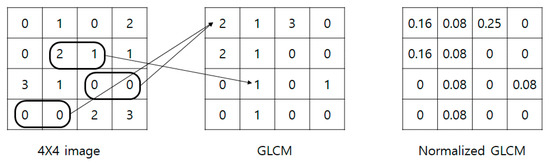
Figure 1.
Process of generating a gray level co-occurrence matrix (GLCM).
Haralick texture [55,56,57,58] is a representative value that is expressed as a single real number like an average or a determinant obtained based on the GLCM. The GLCM Haralick texture was created from the need to use flat images for extracting features from three-dimensional elements that cannot be touched or directly extracted in part. As such, it is effective for obtaining features from retinas that cannot be directly touched or partially extracted.
3.2. Retinal Image
Retina images are digital images of the interior of the eye, specifically the rear portion. Retina images are required to show the retina, optic disk, and blood vessels, as shown in Figure 2. Figure 2 shows a retina image from the digital retinal images for vessel extraction (DRIVE) [59] dataset, which is often used in retina-related studies.
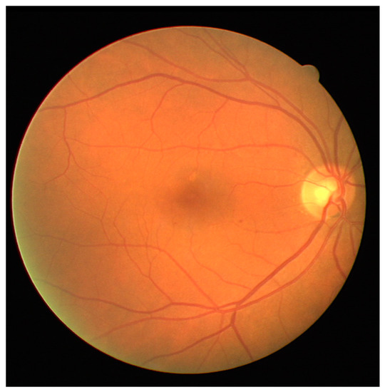
Figure 2.
Example of a retinal image in digital retinal images for vessel extraction (DRIVE).
Many studies have endeavored to automate the extraction of vessels from retina images and to improve the efficiency and accuracy of retinal diagnoses [43]. If a retinal image’s quality is low, the state of the patient’s retina cannot be sufficiently reflected. For example, in the case of diabetic retinopathy, which is the world’s most common diabetic eye disease and a major cause of blindness, one of the criteria for diagnosing the progress of the disease is angiogenesis, in which tiny new vessels grow due to vessel occlusion. If the image quality is low, very fine angiogenesis cannot be seen. Figure 3 shows angiogenesis that has occurred due to diabetic retinopathy. When the resolution of a retinal examination’s output images is poor, considerable money may be spent on readily requesting images for reconfirmation. When a patient with expert knowledge of the eyes has doubts about the physician’s diagnosis regarding their retina images, clear retina images can act as a basis for a re-diagnosis. They may also be helpful in future studies for automating retina image-based diagnostics. However, if the patient does not readily receive high-quality images, the value of the retinal examination may be negligible, and the examination results may be questionable.
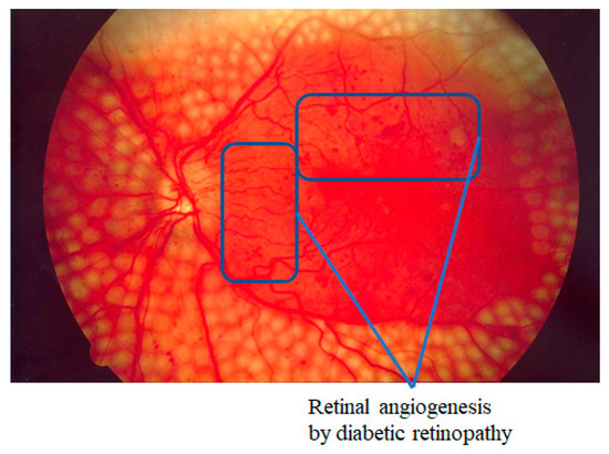
Figure 3.
Example of angiogenesis by diabetic retinopathy.
The techniques that are often used for automating retinal vessel segmentation are based on machine learning [28,29,30,31,32,33,34,35,36,37,38,39,40,41,42,43,44,45,46]. This is because replacing the lost vessel portion of an original retina image with another person’s vessels lacks ethical credibility. On the other hand, machine learning is credible because it learns patterns in which people’s vessels are spread. The focus of most recent studies is on deep learning-based supervised learning, and this is the same for retinal vessel segmentation automation. To learn vessel images, masks must be prepared in advance for the vessel portion. Figure 4 shows the manually prepared vessel portion of Figure 2. Moreover, the areas of the vessels must be specified when the dataset’s retina images are in a different environment (minor changes in position that occur when the image is captured). Figure 5 shows the position mask for Figure 2.
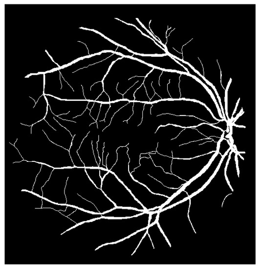
Figure 4.
Retinal vessels of Figure 2.
Figure 5.
Process area of Figure 2.
4. Method
To perform an accurate retinal diagnosis, it is necessary to clearly see the retinal vessels in the images obtained by a retinal examination. Figure 6 illustrates the overall approach. Let us assume that low-quality retinal images (A) have been obtained from a simple retinal examination, such as direct ophthalmoscopy. Low-quality images usually contain blurry portions with clear portions in several parts. Therefore, vessel segmentation is performed only in the clear portions. The low-quality image (A) is used to retrieve the most similar image (B) in the dataset that includes high-quality (clear) vessels, and vessel segmentation is also performed on the retrieved clear image (B). Note that vessel segmentation should only be performed on the clear portions of B (the blurry portions of A). Finally, the identified vessel images are combined to generate a high-resolution image for an accurate retinal diagnosis.
| Algorithm 1 Procedure of the proposed method | |||||
| input: (set of the poor retinal images), (collection of the retinal images) | |||||
| output: (set of the synthesized retinal vessel images) | |||||
| 1 | whilein do | ||||
| 2 | maxSimVal = 0 // maximum similarity value | ||||
| 3 | mostSimImg = null // the most similar image | ||||
| 4 | whilein // find an image which is the most similar with | ||||
| 5 | hs = Haralick similarity(, ) // calculate Haralick similarity between and | ||||
| 6 | if hs > maxSimVal then // select maximum hs | ||||
| 7 | maxSimVal = hs | ||||
| 8 | mostSimImg = | ||||
| 9 | end if | ||||
| 10 | end while | ||||
| 11 | vessel_ = segVessel() // vessel segmentation for | ||||
| 12 | vessel_msi = segVessel(mostSimImg) // vessel segmentation for mostSimImg | ||||
| 13 | thrsh_ = OtsuThreshold(vessel_) // dynamic thresholding for vessel_ | ||||
| 14 | thrsh_msi = OtsuThreshold(vessel_msi) // dynamic thresholding for vessel_msi | ||||
| 15 | mask = bulidMask(thrsh_, thrsh_msi) // build the mask based on thresholding result | ||||
| 16 | while row in .rowsize do // build the synthesized vessel image | ||||
| 17 | while col in .colsize do | ||||
| 18 | if mask.pixel[row][col] = 0 then // if the pixel value is 0, a pixel of original image is imported | ||||
| 19 | vessel_synth[row][col] = vessel_.pixel[row][col] | ||||
| 20 | else // if the pixel value is 1, a pixel of similar image is imported | ||||
| 21 | vessel_synth[row][col] = vessel_msi[row][col] | ||||
| 22 | end if | ||||
| 23 | end while | ||||
| 24 | end while | ||||
| 25 | end while | ||||
| 26 | Return // return set of vessel_synth | ||||
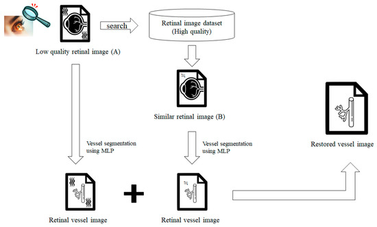
Figure 6.
Overall approach.
Algorithm 1 shows the procedure of the proposed technique. As inputs of the algorithm, is a set of low-quality images in which the user expects to increase quality, and is a set of high-quality retinal image data collected to improve the quality of . Lines 4–10 show the process of finding an image similar to a low-quality retinal image in a data collection. Haralick similarity is used to find the image with the highest similarity to the input low-quality retinal image. The searched similar image is a source of good pixels to replace bad pixels (pixels that cause deterioration in quality) of the original image. This process is covered in detail in Section 4.1. Lines 11–12 show the process of dividing the blood vessel from the retinal image. The blood vessel is divided based on the learned MLP using the DRIVE dataset. This process is covered in detail in Section 4.2. Lines 13–26 show the process of creating a synthesized image by applying a mask. A threshold is used to create a mask with the criteria of noise to be properly removed. In our approach, the Otsu method [60,61,62,63,64,65,66,67,68,69] is applied to dynamically select the threshold. After the mask generation is completed, a pixel value is determined for each pixel of the mask. If the pixel value is 0, the pixel of the original image is fetched, and if 1, the pixel of the similar image is fetched. The final synthesized results are returned as a set. This process is covered in detail in Section 4.3.
The proposed approach consists of three stages: searching for similar images, segmenting retinal vessels, and combining images. Each stage is described in detail in the following subsections.
4.1. Searching for Similar Images
For the proposed technique, the degraded (low-quality) retinal images are inputted, and images are found that are the most similar to the input images in the pre-constructed retinal image data set, which only contains high-quality retinal images. The criteria for finding similar images are based on a logistic regression analysis [70,71,72,73] of Haralick textures, which are the GLCM matrix calculation results. These are used because the appearances of most retinas are similar, and therefore, finding features is difficult, as different patient retinal images cannot be distinguished without expert ophthalmology knowledge. GLCM-based Haralick textures are useful for determining similarities between retinal images because they are based on pixel changes. The proposed method uses a Haralick texture logistic regression process to find the similarity between the bad and dataset images. It then selects the image with the maximum similarity with the next input image.
4.2. Segmenting Retinal Vessels
During this stage, vessel segmentation is performed on the low-quality (low-resolution) retina and similar images. MLP, which uses an artificial neural network algorithm based on supervised learning, is employed for the vessel segmentation. Since MLP is a universal approximator, all functions can be represented if the MLP model consists of a large enough number of neurons and layers. It is also better to find an accurate weight value for every pixel instead of extracting partial features, as the retina images of the people having an average retina are not that different.
MLP receives the image pixels as the input. Each input is multiplied by the weight of the edges and added. Next, the activation function is used on the results to determine how much they affect the next node, and this is transferred to the next layer. This is summarized by Equation (1), where is the input image pixels, is the weight assigned to each edge, and is the node output.
Figure 7 shows a simple example of the MLP method used in this study. The high-resolution fundus (HRF) [74] image dataset contains higher-quality retinal images compared to those of DRIVE, and provides both low- and high-quality retinal images. Figure 8 shows a low-quality retinal image. The bottom part of the image is unclear owing to white noise caused by environmental factors. Figure 9 shows a retinal vessel image created by performing vessel segmentation on Figure 8. The white noise seen in Figure 8 also affects vessel segmentation. Figure 10 is a high-quality retinal image and the white noise observed in Figure 8 has disappeared. The bottom part of the vessel stem is clearly visible, which did not appear in the original image. Figure 11 shows a retinal vessel image created by performing vessel segmentation on Figure 10. Unlike Figure 9, the bottom part of the vessel stem is shown clearly.
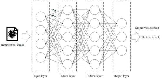
Figure 7.
Process of retinal vessel segmentation using MLP.
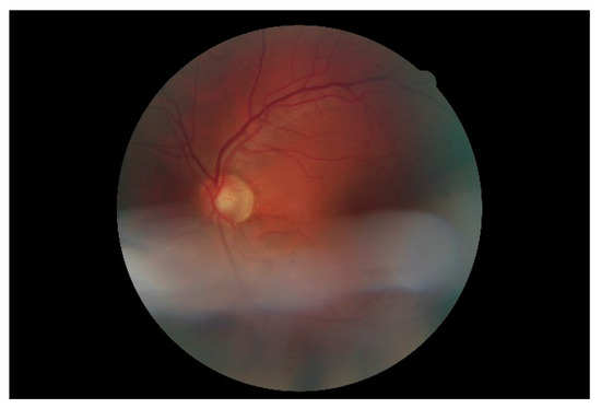
Figure 8.
Retinal image (low quality).
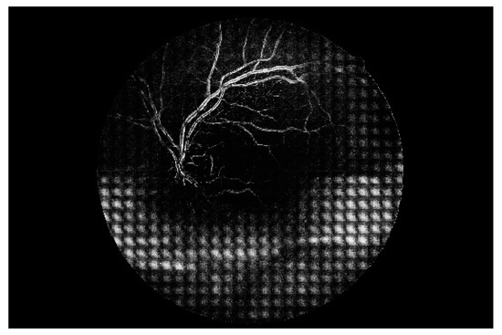
Figure 9.
Retinal vessel image of Figure 8.
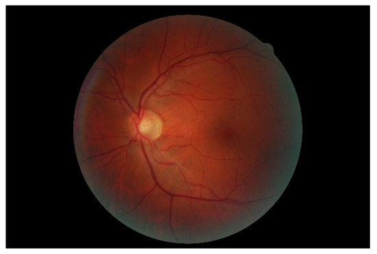
Figure 10.
Retinal image (high quality).
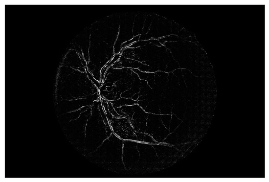
Figure 11.
Retinal vessel image of Figure 10.
4.3. Synthesizing Images
The vessel images obtained from the low-quality (low-resolution) retinal images do not sufficiently show the patient status. Thus, the proposed method can be used to synthesize the original low-quality retinal image with the image that is the most similar to that of the high-resolution vessel image dataset. The mask concept generally used in computer vision techniques is applied to synthesize the low-quality input and similar images. The proposed method must satisfy three constraints to obtain a safe synthesis. The constraints are as follows.
- Removal of noise mixed with the bad image.
- Express damaged vessels owing to low quality.
- Does not damage remaining vessels in the bad image.
To synthesize two images, a mask is created by setting a threshold value for the gray levels of both the original low-quality and similar images. Areas with gray levels below and above the threshold are set to 0 and 1, respectively, to create a binary image in advance. The binary image is used as the input for the mask equation. The pixels of the grayscale images are used to create a new synthetic image. The mask pixel (, ) equation is as follows:
A pixel of the original (low-quality) image is inserted into the synthesized image when the mask is set to 0. On the other hand, a pixel of the similar image is inserted into the synthesis image when the mask is set to 1.
Constraint (1) assumes that a pixel (a, b) of the low-quality image is noise. If this is so, then the mask is set to 1 by constraint (1), and the proposed method uses the similar image pixel. As the original image pixel (a, b) is noise, the similar image pixel (a, b) is clean. Therefore, the proposed method satisfies constraint (1). Constraint (2) assumes that the original image pixel (a, b) is damaged and is part of the vessel that is not shown. If the dataset sufficiently guarantees that the similar image is similar to the low-quality image (i.e., the low-quality image is a favorable state), the similar image pixel (a, b) is set to 1, and therefore, the mask is set to 1. As such, the proposed method satisfies constraint (2). Constraint (3) assumes that pixel (a, b) is part of the properly depicted vessel, and that the similar image pixel (a, b) is also part of the vessel. Therefore, the proposed method satisfies constraint (3). It is assumed that pixel (a, b) is part of a blank area without noise in the low-quality image. Then, pixel (a, b) of the similar image is also part of a blank area without noise. Thus, the mask is set to 0.
Once the mask-generating process for the pair consisting of an image and a similar image has been completed, the proposed technique will be employed to create a restored (synthesized) image based on the mask. The pixel value (, ) value of restored image imports the pixel value (, ) of the bad or the similar image. If the pixel value (, ) of the mask is 1, the restored image imports similar (good) image value (i, ), whereas if the pixel value (,) of the mask is 0, the restored image imports the bad (original) image value (, ). That is, the restored image imports the similar image’s pixel for the main branch or the noise, or imports the original image’s pixel for the sub-branches as the sub-branches are excluded by threshold function. The final restored (synthesized) image is shown in Figure 12.
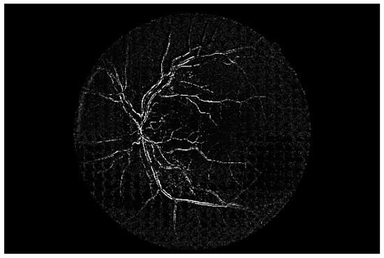
Figure 12.
Synthesis result.
5. Evaluation
To evaluate the proposed method, we collected retinal images from the DRIVE and HRF datasets (These data sets are available as presented in Supplementary Materials). DRIVE is a retinal image dataset that has been used in many retinal image classification and vessel segmentation studies. DRIVE consists of 140 retinal images. Since DRIVE provides 2 manual vessel masks per retina image, the user does not need to make blood vessel masks separately and can choose a mask that produces a more accurate result from the two makes for each image. Thus, it is more reasonable to use DRIVE for a training set. Using DRIVE makes this study comparable to the other studies. HRF has a higher image quality than DRIVE in general. Although HRF does not provide a blood vessel mask, it contains both high- and low-quality retinal images, making it useful for the evaluation of the proposed approach. HRF consists of 18 high- and low-quality retinal image pairs and due to the characteristics of HRF that does not provide any masks, it is more reasonable for it to be used for a testing set. As the performance of the proposed method might change following the accuracy of the similar image representing a patient’s retina image, it is better to have more images in the dataset. In this experiment, we assume that the retinal images of all people with normal retinas are similar.
It has been known that there are not any specific values that meet the number of nodes or layers appropriate for all situations or datasets. Thus, we needed to find the appropriate numbers for both nodes and layers and found them by constructing the MLP models having a different number of nodes and layers manually. As a result, we realized that 3 hidden layers and 1.8–2 times nodes of the input layer were sufficient enough.
As the noise removal performance by the proposed technique can be affected by the threshold values used when defining a mask, we evaluated the noise removal performance of each threshold value to achieve the optimal noise removal performance level possible. Each pixel in an input image converted with a gray scale has 256 levels, indicating that the color would become darker as it approaches near 0 or vice versa. For the threshold function, all the pixels having a gray-scale level exceeding the parameter value were set to 255, whereas the opposite ones were set to 0. Figure 13 shows the masks generated from the six threshold types in the image in Figure 9. Since the area indicated as 1 (yellow section) due to the mask applied with a threshold type would import the pixel of a similar image, the mask that represents the area of the noise (i.e., the yellow section) more clearly will be deemed as a good mask.
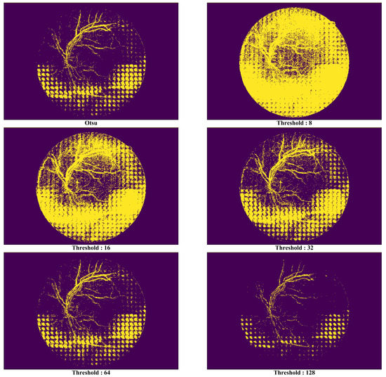
Figure 13.
Comparison of synthetic vessel images by threshold types.
In Figure 13, it is possible to know in the picture that there is no significant meaning in the areas distinguished by the mask as most their pixel values are 1 when the threshold value is 8. Although such a phenomenon had decreased when the threshold value was increased from 16 to 32, the areas that had been excessively identified as noise existed at the top of the image. The optimal performance was seen when the threshold value was 64, but it became harder to distinguish the noise areas as the value exceeded it.
For this study, the Otsu method [60,61,62,63,64,65,66,67,68,69] was applied to select reliably threshold value that has a great influence on the synthesized results of the proposed approach. The Otsu method provides the criteria for setting the most natural threshold value using a statistical method. This method defines two variances for a threshold value, , which could be from 0 to 255.
where is the ratio of pixels darker than the value, and is the ratio of pixels brighter than the value. is the variance of pixels darker than the value, and is the variance of pixels brighter than the value. is the average brightness of the pixels darker than the value, and is the average brightness of the pixels brighter than the value. The Otsu method is to select with the largest inter-class variance when pixels are divided into two classes based on while increasing the threshold value from the minimum value to the maximum value (from 0 to 255). That is, the Otsu method minimizes (3) or maximizes (4) to dynamically find the optimal threshold (this method tries to maintain a small variance inside the group, and groups divided by try to maintain a large variance).
Figure 14 shows a comparison of a vessel image extracted from the original low-quality image with one synthesized by the proposed method. The white noise area at the bottom of the original low-quality image is clearly not present in the synthesized vessel image. As for the bottom part of the vessel stem that was damaged and could not be distinguished, this was created independently with noise removal.
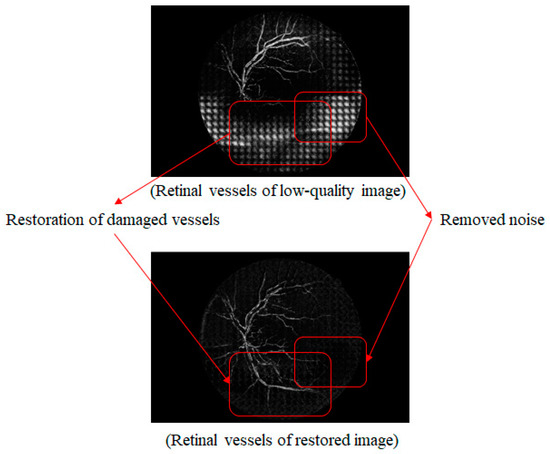
Figure 14.
Comparison of low-quality retinal and synthetic vessel images.
Figure 15 shows a comparison of the vessel image extracted from the original high-quality image with one synthesized by the proposed method. The vessel portion that was newly created in the synthesized vessel image is similar to the vessels in the original high-quality image. However, compared to the original high-quality image, the right part of the vessel is not clean, and there is faint noise in the vessel image that was synthesized by the proposed method. The noise is below the threshold value that was set when the mask was created. Even though the area below the threshold value is noise, the pixels from the original low-quality image are used because it was recognized as an empty area and was set to 0 in the binary image. However, owing to this reason, merely lowering the threshold value increases the effects of the similar image. This makes it possible to ignore the empty parts in the low-quality image and vessels can be used that are not related to the owner of the original image.
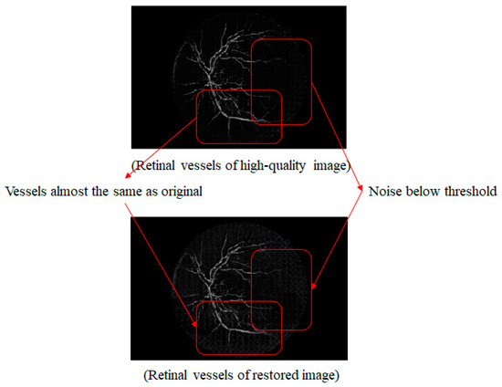
Figure 15.
Comparison of high-quality retinal and synthetic vessel images.
In our evaluation, we focused on the two types of the comparisons: (1) a comparison of the low-quality vessel image with the high-quality vessel image, and (2) a comparison of the low-quality vessel image with the restored image by the proposed method using the HRF dataset. A statistical analysis was performed on the experimental results to objectively assess the proposed method. An independent sample t-test is often used to compare the population means of two groups, mainly to observe the similarities or differences between two different test groups [75,76,77,78]. In our experiment, an independent sample t-test was used to determine if there was a significant difference between the high-quality and synthesized images. For the evaluation, we conducted three experiments using independent sample t-test for the three separate techniques: (1) analysis of feature matching, (2) analysis of image similarity based on the Haralick algorithm, (3) analysis of mean-square error (MSE). We checked whether these two groups (low-quality image vs. high-quality image and low-quality vs. the restored image) had an equal variance prior to performing the t-test. Thus, we conducted the F-test first and then checked whether the p-value was greater than the significant level (0.05).
Table 1 shows the number of high-quality and restored (synthesized) image features that match those of the low-quality image using feature matching. In Table 1, the “# of features matched in bad–good images” represents the number of matching features obtained when the feature-matching algorithm was used on the low- and high-quality-images. The “# of features matched in bad–synthesized image” represents the number of matching features obtained when the feature-matching algorithm was used on the low-quality and synthesized images.

Table 1.
Comparative analysis from feature matching.
Table 2 shows that the retrieved high-quality and restored (synthesized) images are similar to the low-quality images. In Table 2, “Bad–Good Image Similarity” represents the similarity when the Haralick algorithm was used on the low-quality and good images. The “Bad–Synthesized Image Similarity” represents the similarity when the Haralick algorithm was used on the low-quality and synthesized images.
Table 2.
Comparative analysis to validate synthetic images using Haralick algorithm.
The p-value exceeded the significance level of 0.05 for the independent sample t-test results. Thus, there were no statistically significant differences between the high-quality and synthesized images.
In entries 1, 12, and 18 of Table 2, the similarity of the low- and high-quality images was greater than that of the low-quality and synthesized images, unlike the majority of cases. This is because the similar images used in the image synthesis did not adequately represent the original images. As such, this appears to be a problem that will be resolved by improving the dataset or the algorithm used to find similar images.
Table 3 shows how many high-quality and restored (synthesized) images are different with the low-quality images through mean-square error (MSE). In Table 3, the “MSE Between Bad–Good Image” represents the MSE value when the MSE algorithm was used for the low-quality images and the high-quality images. In addition, the “MSE Between Bad–Synthesized Image” represents the MSE value when the MSE algorithm was used for the low-quality images and the synthesized images.
Table 3.
Comparative analysis from mean-square error (MSE).
Figure 16 shows the six p-values obtained from the experiments (i.e., 2 types of tests and 3 experiments). Here, the Y axis represents the p-values of the tests, whereas the black bar and slash-patterned bar represent the F-test and T-test, respectively. The results from the three experiments showed that there was no difference between the good image and the synthesized image. In all experiments, two groups (low-quality image vs. high-quality image and low-quality vs. the synthesized image) had an equal variance as F-test p-values were greater than the significant level (0.05). Moreover, since all the t-test p-values were greater than the significant level (0.05) in all experiments, we were able to assume that there was no significant difference between the two groups, confirming that the synthesized retina image was similar enough with the good quality retina image.
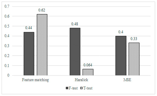
Figure 16.
Statistical analysis for high-quality retinal and synthetic vessel images.
In addition, for the three types of experiments, we have also evaluated how the threshold values affected the p-values. Table 4 shows how the p-values had changed according to the changes in the threshold types: Otsu method and Global values (8 to 128). The result showed that for the global threshold, the p-values also increased following the increase in the threshold values but they dropped drastically when the latter reached 128. As previously mentioned, this might have been caused as the noise was not clearly removed when the threshold value had become excessively higher. Especially, in a similarity test with a Haralick algorithm, all the p-values could not exceed the significance level of 0.05 except when the threshold value was 64. As the picture shows, the p-value in an extreme situation, having a threshold value of 8, for example, decreases less when compared with another extreme situation where the threshold value is 128. This means that it is better to use the similar image as it is instead of using a low-quality image. Since the synthesized image will become closer to a similar image as the number of areas having a pixel value of 1 (i.e., a low threshold value) increases, it would represent the actual retinal image of a patient more clearly when the dataset is organized in a better way, which means that the lower threshold values would reduce damage to the synthesized image.
Table 4.
p-value changes by threshold types.
In the case of the threshold derived by the Otsu method, the p-value obtained from the feature matching was similar to the manually selected global threshold. However, the p-value generated by the Haralick algorithm and MSE was higher than the manually selected global threshold. In our experiments, it was confirmed that the Otsu method was a very appropriate threshold setting method for the Haralick algorithm and MSE.
6. Discussion
An image synthesis approach was proposed in this study to improve the quality of retinal images, particularly their vessel areas, to help physicians perform diagnoses after retinal examinations. As this is a medical study, the proposed method will be very useful for emergency medical situations requiring high-quality images in real time.
Table 5 shows the time taken to perform 10 repeated rounds of training and testing for the experiments described in Section 4. For the 10 rounds of data, the smallest value is marked in bold, and the largest value is underlined. The average training time was 634 s, and in all cases, it took approximately 10 min. The average testing time was approximately 33 s, and in all cases, it took approximately 30 s. The training time is not a significant issue as this is the processing time required by the server. The problem is the testing time, as this is the time taken to produce results after a physician has inputted a newly created retinal image into the trained model, and it has the greatest effect on real-time service. Nevertheless, an average of 30 s is sufficient for situations with soft real-time conditions. However, it is difficult for our approach to satisfy hard real-time conditions such as life-threatening emergency medical situations.
Table 5.
Time for generating synthetic vessel images (The minimum value in each column is presented in bold, and the maximum value in each column is underlined).
7. Conclusions
This study has proposed an image synthesis method that allows for accurate diagnoses after retinal examinations. The proposed method ensures that it is always possible to clearly distinguish the vessel portions of images that are essential for examinations even when the images that were obtained in the retinal examination have a low resolution. Specifically, it collects the most similar images from a dataset that stores existing high-resolution images, segments the high-resolution vessel portions, and combines them with the low-quality (low-resolution) retinal image to obtain the clearest vessel image. Through this process, optimal high-resolution vessel images, which can aid in making accurate diagnoses, are extracted.
In addition, this type of study contributes toward future research by formulating a complex retina vessel structure model from an anatomic and ophthalmological perspective. When a patient with expert knowledge of the eyes has doubts about the physician’s diagnosis regarding their retinal images, clear retinal images can act as a basis for a re-diagnosis. Our results also contribute toward future studies on automating retinal image-based diagnoses.
Future directions for this study are as follows. As discussed in Section 6, the current method cannot provide the critical real-time services that are needed in emergency medical situations. We believe that it is very important to study this first. In addition, this study’s dataset follows a fixed form, and the method cannot dynamically handle a variety of datasets. This does not reflect reality, and retina data formats can vary according to the country or type of hospital. To deal with this, we will study data reduction techniques that are based on the characteristics of retina images. By doing so, it will be possible to dynamically handle different retinal data formats. Moreover, studies on efficiently generating retinal data are expected to contribute toward improving the quality of the retinal images themselves rather than efficient retinal data structures.
Supplementary Materials
The datasets used during the current study are available from the following websites (DRIVE: https://drive.grand-challenge.org/ and HRF: https://www5.cs.fau.de/research/data/fundus-images/).
Author Contributions
Conceptualization, D.-G.L. and Y.-S.S.; Data curation, D.-G.L.; Formal analysis, Y.J. and Y.-S.S.; Funding acquisition, Y.-S.S.; Investigation, Y.J.; Methodology, D.-G.L., Y.J. and Y.-S.S.; Project administration, Y.-S.S.; Resources, D.-G.L.; Software, D.-G.L.; Supervision, Y.J. and Y.-S.S.; Validation, D.-G.L., Y.J. and Y.-S.S.; Visualization, D.-G.L. and Y.J.; Writing—original draft, D.-G.L., Y.J. and Y.-S.S.; Writing—review & editing, D.-G.L., Y.J. and Y.-S.S. All authors have read and agreed to the published version of the manuscript.
Funding
This work was supported by the 2020 Yeungnam University Research Grant.
Conflicts of Interest
The authors declare no conflicts of interest.
Abbreviations
| MLP | Multi-Layer Perceptron |
| FFDNN | Feed-Forward Deep Neural Network |
| GANs | Generative Adversarial Networks |
| CNN | Convolutional Neural Network |
| GLCM | Gray Level Co-occurrence Matrix |
| DRIVE | Digital Retinal Images for Vessel Extraction |
| HRF | High-Resolution Fundus |
| STARE | Structured Analysis of the Retina |
References
- McGrory, S.; Cameron, J.R.; Pellegrini, E.; Warren, C.; Doubal, F.N.; Deary, I.J.; Dhillon, B.; Wardlaw, J.M.; Trucco, E.; MacGillivray, T.J. The application of retinal fundus camera imaging in dementia: A systematic review. Alzheimer’s Dement. Diagn. Assess. Dis. Monit. 2017, 6, 91–107. [Google Scholar] [CrossRef]
- Sandeep, C.S.; Kumar, S.A.; Mahadevan, K.; Manoj, P. A Comparative Study between Fundus Imaging and Optical Coherence Tomography for the Early Diagnosis of Alzheimer’s Disease. MOJ Appl. Bionics Biomech. 2017, 6, 201–204. [Google Scholar]
- Sandeep, C.S.; Kumar, S.A.; Mahadevan, K.; Manoj, P. Early prognosis of Alzheimer’s disease using images from fundus camera. In Proceedings of the 2017 IEEE International Conference on Electrical. Instrumentation and Communication Engineering (ICEICE), Karur, India, 27–28 April 2017; pp. 1–5. [Google Scholar]
- MacGillivray, T.; McGrory, S.; Pearson, T.; Cameron, J. Retinal Imaging in Early Alzheimer’s Disease. Biomark. Preclin. Alzheimer’s Dis. 2018, 137, 199–212. [Google Scholar]
- Michigan Medicine. Available online: https://www.uofmhealth.org/health-library/hw5223 (accessed on 22 April 2020).
- Lee, J.S. Primary Eye Examination; Springer: Berlin/Heidelberg, Germany, 2019; pp. 101–111. [Google Scholar]
- Tang, J.; Deng, C.; Huang, G.B. Extreme learning machine for multilayer perceptron. IEEE Trans. Neural Netw. Learn. Syst. 2015, 27, 809–821. [Google Scholar] [CrossRef] [PubMed]
- Heidari, A.A.; Faris, H.; Aljarah, I.; Mirjalili, S. An efficient hybrid multilayer perceptron neural network with grasshopper optimization. Soft Comput. 2019, 23, 7941–7958. [Google Scholar] [CrossRef]
- Huh, J.-H. Big Data Analysis for Personalized Health Activities: Machine Learning Processing for Automatic Keyword Extraction Approach. Symmetry 2018, 10, 93. [Google Scholar] [CrossRef]
- Abràmoff, M.D.; Garvin, M.K.; Sonka, M. Retinal imaging and image analysis. IEEE Rev. Biomed. Eng. 2010, 3, 169–208. [Google Scholar] [CrossRef]
- Kaur, J.; Mittal, D. A generalized method for the segmentation of exudates from pathological retinal fundus images. Biocybern. Biomed. Eng. 2018, 38, 27–53. [Google Scholar] [CrossRef]
- Soorya, M.; Issac, A.; Dutta, M.K. An automated and robust image processing algorithm for glaucoma diagnosis from fundus images using novel blood vessel tracking and bend point detection. Int. J. Med Inform. 2018, 110, 52–70. [Google Scholar]
- Ma, W.; Yu, S.; Ma, K.; Wang, J.; Ding, X.; Zheng, Y. Multi-task Neural Networks with Spatial Activation for Retinal Vessel Segmentation and Artery/Vein Classification. In Proceedings of the International Conference on Medical Image Computing and Computer-Assisted Intervention, Shenzhen, China, 13–17 October 2019; pp. 769–778. [Google Scholar]
- Yin, P.; Wu, Q.; Xu, Y.; Min, H.; Yang, M.; Zhang, Y.; Tan, M. PM-Net: Pyramid Multi-label Network for Joint Optic Disc and Cup Segmentation. In Proceedings of the International Conference on Medical Image Computing and Computer-Assisted Intervention, Shenzhen, China, 13–17 October 2019; pp. 129–137. [Google Scholar]
- Powles, J.; Hodson, H. Google DeepMind and healthcare in an age of algorithms. Health Technol. 2017, 7, 351–367. [Google Scholar] [CrossRef]
- Zhou, Y.; Wang, B.; He, X.; Cui, S.; Zhu, F.; Liu, L.; Shao, L. DR-GAN: Conditional Generative Adversarial Network for Fine-Grained Lesion Synthesis on Diabetic Retinopathy Images. arXiv 2019, arXiv:1912.04670. [Google Scholar]
- Foracchia, M.; Grisan, E.; Ruggeri, A. Luminosity and contrast normalization in retinal images. Med. Image Anal. 2005, 9, 179–190. [Google Scholar] [CrossRef] [PubMed]
- Mitra, A.; Roy, S.; Roy, S.; Setua, S.K. Enhancement and restoration of non-uniform illuminated fundus image of retina obtained through thin layer of cataract. Comput. Methods Programs Biomed. 2018, 156, 169–178. [Google Scholar] [CrossRef] [PubMed]
- Zhou, M.; Jin, K.; Wang, S.; Ye, J.; Qian, D. Color retinal image enhancement based on luminosity and contrast adjustment. IEEE Trans. Biomed. Eng. 2017, 65, 521–527. [Google Scholar] [CrossRef]
- Gupta, B.; Tiwari, M. Minimum mean brightness error contrast enhancement of color images using adaptive gamma correction with color preserving framework. Optik 2016, 127, 1671–1676. [Google Scholar] [CrossRef]
- Gupta, B.; Tiwari, M. Color retinal image enhancement using luminosity and quantile based contrast enhancement. Multidimens. Syst. Signal Process. 2019, 30, 1829–1837. [Google Scholar] [CrossRef]
- Cao, L.; Li, H.; Zhang, Y. Retinal image enhancement using low-pass filtering and α-rooting. Signal Process. 2020, 170, 1–12. [Google Scholar] [CrossRef]
- Kaggle Diabetic Retinopathy Detection Challenge. Available online: https://www.kaggle.com/c/diabetic-retinopathy-detection (accessed on 22 April 2020).
- Xiong, L.; Li, H.; Xu, L. An enhancement method for color retinal images based on image formation model. Comput. Methods Programs Biomed. 2017, 143, 137–150. [Google Scholar] [CrossRef]
- Decencière, E.; Zhang, X.; Cazuguel, G.; Lay, B.; Cochener, B.; Trone, C.; Gain, P.; Ordonez, R.; Massin, P.; Erginay, A.; et al. Feedback on a publicly distributed image database: The Messidor database. Image Anal. Stereol. 2014, 33, 231–234. [Google Scholar] [CrossRef]
- Zhao, H.; Li, H.; Maurer-Stroh, S.; Cheng, L. Synthesizing retinal and neuronal images with generative adversarial nets. Med. Image Anal. 2018, 49, 14–26. [Google Scholar] [CrossRef]
- Niu, Y.; Gu, L.; Lu, F.; Lv, F.; Wang, Z.; Sato, I.; Zhang, Z.; Xiao, Y.; Dai, X.; Cheng, T. Pathological evidence exploration in deep retinal image diagnosis. In Proceedings of the AAAI Conference on Artificial Intelligence, Honolulu, HI, USA, 27 January–1 February 2019; pp. 1093–1101. [Google Scholar]
- Costa, P.; Galdran, A.; Meyer, M.I.; Niemeijer, M.; Abramoff, M.; Mendonca, A.M.; Campilho, A. End-to-end adversarial retinal image synthesis. IEEE Trans. Med. Imaging 2017, 37, 781–791. [Google Scholar] [CrossRef] [PubMed]
- Liskowski, P.; Krawiec, K. Segmenting retinal blood vessels with deep neural networks. IEEE Trans. Med. Imaging 2016, 35, 2369–2380. [Google Scholar] [CrossRef] [PubMed]
- Huh, J.H. Smart Grid Test Bed using OPNET and Power Line Communication; IGI Global: Hershey PA, USA, 2018; pp. 1–21. [Google Scholar]
- Gulshan, V.; Peng, L.; Coram, M.; Stumpe, M.C.; Wu, D.; Narayanaswamy, A.; Venugopalan, S.; Widner, K.; Madams, T.; Cuadros, J. Development and validation of a deep learning algorithm for detection of diabetic retinopathy in retinal fundus photographs. JAMA 2016, 316, 2402–2410. [Google Scholar] [CrossRef] [PubMed]
- Huh, J.H. PLC-based design of monitoring system for ICT-integrated vertical fish farm. Hum. Cent. Comput. Inf. Sci. 2017, 7, 1–19. [Google Scholar] [CrossRef]
- Gargeya, R.; Leng, T. Automated identification of diabetic retinopathy using deep learning. Ophthalmology 2017, 124, 962–969. [Google Scholar] [CrossRef]
- Huh, J.H.; Seo, K. A preliminary analysis model of big data for prevention of bioaccumulation of heavy metal-based pollutants: Focusing on the atmospheric data analyses for smart farm. Contemp. Eng. Sci. 2016, 9, 1447–1462. [Google Scholar] [CrossRef]
- Poplin, R.; Varadarajan, A.V.; Blumer, K.; Liu, Y.; McConnell, M.V.; Corrado, G.S.; Peng, L.; Webster, D.R. Prediction of cardiovascular risk factors from retinal fundus photographs via deep learning. Ophthalmology 2017, 124, 962–969. [Google Scholar] [CrossRef]
- Huh, J.H.; Koh, T.; Seo, K. Design of a shipboard outside communication network and the test bed using PLC: For the Workers’ safety management during ship-building process. In Proceedings of the 10th International Conference on Ubiquitous Information Management and Communication, Danang, Vietnam, 4–6 January 2016; pp. 1–6. [Google Scholar]
- Fu, H.; Xu, Y.; Wong, D.W.K.; Liu, J. Retinal vessel segmentation via deep learning network and fully-connected conditional random fields. In Proceedings of the 2016 IEEE 13th International Symposium on Biomedical Imaging (ISBI), Prague, Czech Republic, 13–16 April 2016; pp. 781–791. [Google Scholar]
- Barkana, B.D.; Saricicek, I.; Yildirim, B. Performance analysis of descriptive statistical features in retinal vessel segmentation via fuzzy logic, ANN, SVM, and classifier fusion. IEEE Trans. Med. Imaging 2017, 118, 165–176. [Google Scholar] [CrossRef]
- Li, Q.; Feng, B.; Xie, L.; Liang, P.; Zhang, H.; Wang, T. A cross-modality learning approach for vessel segmentation in retinal images. IEEE Trans. Med. Imaging 2015, 35, 109–118. [Google Scholar] [CrossRef]
- Zhu, C.; Zou, B.; Zhao, R.; Cui, J.; Duan, X.; Chen, Z.; Liang, Y. Retinal vessel segmentation in colour fundus images using Extreme Learning Machine. IEEE Trans. Med. Imaging 2017, 55, 68–77. [Google Scholar] [CrossRef]
- Aslani, S.; Sarnel, H. A new supervised retinal vessel segmentation method based on robust hybrid features. IEEE Trans. Med. Imaging 2016, 30, 1–12. [Google Scholar] [CrossRef]
- Ben-Cohen, A.; Mark, D.; Kovler, I.; Zur, D.; Barak, A.; Iglicki, M.; Soferman, R. Retinal Layers Segmentation Using Fully Convolutional Network in OCT Images. Available online: https://www.rsipvision.com/wp-content/uploads/2017/06/Retinal-Layers-Segmentation.pdf (accessed on 11 March 2020).
- Tennakoon, R.; Gostar, A.K.; Hoseinnezhad, R.; Bab-Hadiashar, A. Retinal fluid segmentation in OCT images using adversarial loss based convolutional neural networks. In Proceedings of the 2018 IEEE 15th International Symposium on Biomedical Imaging, Washington, DC, USA, 4–7 April 2018; pp. 1436–1440. [Google Scholar]
- Wang, S.; Yin, Y.; Cao, G.; Wei, B.; Zheng, Y.; Yang, G. Hierarchical retinal blood vessel segmentation based on feature and ensemble learning. Neurocomputing 2015, 149, 708–717. [Google Scholar] [CrossRef]
- Oliveira, A.; Pereira, S.; Silva, C.A. Retinal vessel segmentation based on fully convolutional neural networks. Expert Syst. Appl. 2018, 112, 229–242. [Google Scholar] [CrossRef]
- Ronneberger, O.; Fischer, P.; Brox, T. U-net: Convolutional networks for biomedical image segmentation. In Proceedings of the International Conference on Medical Image Computing and Computer-Assisted Intervention, Munich, Germany, 5–9 October 2015; pp. 234–241. [Google Scholar]
- Marrugo, A.G.; Millan, M.S.; Sorel, M.; Sroubek, F. Retinal image restoration by means of blind deconvolution. J. Biomed. Opt. 2011, 16, 116016. [Google Scholar] [CrossRef]
- Nguyen, U.T.V.; Bhuiyan, A.; Park, L.A.F.; Ramamohanarao, K. An effective retinal blood vessel segmentation method using multi-scale line detection. Pattern Recognit. 2013, 46, 703–715. [Google Scholar] [CrossRef]
- Dias, J.M.P.; Oliveira, C.M.; da Silva Cruz, L.A. Retinal image quality assessment using generic image quality indicators. Inf. Fusion 2014, 19, 73–90. [Google Scholar] [CrossRef]
- Zhang, J.; Dashtbozorg, B.; Bekkers, E.; Pluim, J.P.W.; Duits, R.; ter Haar Romeny, B.M. Robust retinal vessel segmentation via locally adaptive derivative frames in orientation scores. IEEE Trans. Med. Imaging 2016, 35, 2631–2644. [Google Scholar] [CrossRef]
- Zhang, X.; Cui, J.; Wang, W.; Lin, C. A study for texture feature extraction of high-resolution satellite images based on a direction measure and gray level co-occurrence matrix fusion algorithm. Sensors 2017, 17, 1474. [Google Scholar] [CrossRef]
- Mishra, S.; Majhi, B.; Sa, P.K.; Sharma, L. Gray level co-occurrence matrix and random forest based acute lymphoblastic leukemia detection. Biomed. Signal Process. Control 2017, 33, 272–280. [Google Scholar] [CrossRef]
- Xiao, F.; Kaiyuan, L.; Qi, W.; Yao, Z.; Xi, Z. Texture analysis based on gray level co-occurrence matrix and its application in fault detection. In Proceedings of the International Geophysical Conference, Beijing, China, 24–27 April 2018; pp. 836–839. [Google Scholar]
- Pare, S.; Bhandari, A.K.; Kumar, A.; Singh, G.K. An optimal color image multilevel thresholding technique using grey-level co-occurrence matrix. Expert Syst. Appl. 2017, 87, 335–362. [Google Scholar] [CrossRef]
- Wibmer, A.; Hricak, H.; Gondo, T.; Matsumoto, K.; Veeraraghavan, H.; Fehr, D.; Zheng, J.; Goldman, D.; Moskowitz, C.; Fine, S.W. Haralick texture analysis of prostate MRI: Utility for differentiating non-cancerous prostate from prostate cancer and differentiating prostate cancers with different Gleason scores. Eur. Radiol. 2015, 25, 2840–2850. [Google Scholar] [CrossRef] [PubMed]
- Vrbik, I.; Van Nest, S.J.; Meksiarun, P.; Loeppky, J.; Brolo, A.; Lum, J.J.; Jirasek, A. Haralick texture feature analysis for quantifying radiation response heterogeneity in murine models observed using Raman spectroscopic mapping. PLoS ONE 2019, 14, e0212225. [Google Scholar] [CrossRef] [PubMed]
- Lofstedt, T.; Brynolfsson, P.; Asklund, T.; Nyholm, T.; Garpebring, A.A. Gray-level invariant Haralick texture features. PLoS ONE 2019, 14, e0212110. [Google Scholar] [CrossRef] [PubMed]
- Brynolfsson, P.; Nilsson, D.; Torheim, T.; Asklund, T.; Karlsson, C.T.; Trygg, J.; Nyholm, T.; Garpebring, A. Haralick texture features from apparent diffusion coefficient (ADC) MRI images depend on imaging and pre-processing parameters. Sci. Rep. 2017, 7, 1–11. [Google Scholar] [CrossRef] [PubMed]
- Staal, J.; Abramoff, M.D.; Niemeijer, M.; Viergever, M.A.; Van Ginneken, B. Prediction of cardiovascular risk factors from retinal fundus photographs via deep learning. Ophthalmology 2004, 23, 501–509. [Google Scholar]
- Otsu, N. A threshold selection method from gray-level histograms. IEEE Trans. Syst. Man Cybern. 1979, 9, 62–66. [Google Scholar] [CrossRef]
- Martinez-Perez, M.E.; Hughes, A.D.; Thom, S.A.; Bharath, A.A.; Parker, K.H. Segmentation of blood vessels from red-free and fluorescein retinal images. Med. Image Anal. 2007, 11, 47–61. [Google Scholar] [CrossRef]
- Al-Rawi, M.; Qutaishat, M.; Arrar, M. An improved matched filter for blood vessel detection of digital retinal images. Comput. Biol. Med. 2007, 37, 262–267. [Google Scholar] [CrossRef]
- Miri, M.S.; Mahloojifar, A. Retinal image analysis using curvelet transform and multistructure elements morphology by reconstruction. IEEE Trans. Biomed. Eng. 2010, 58, 1183–1192. [Google Scholar] [CrossRef]
- Fu, H.; Xu, Y.; Lin, S.; Wong, D.W.K.; Liu, J. Deepvessel: Retinal vessel segmentation via deep learning and conditional random field. In Proceedings of the International Conference on Medical Image Computing and Computer-Assisted Intervention, Athens, Greece, 17–21 October 2016; pp. 132–139. [Google Scholar]
- Imani, E.; Pourreza, H.R. A novel method for retinal exudate segmentation using signal separation algorithm. Comput. Methods Programs Biomed. 2016, 133, 195–205. [Google Scholar] [CrossRef]
- Liu, Q.; Zou, B.; Chen, J.; Ke, W.; Yue, K.; Chen, Z.; Zhao, G. A location-to-segmentation strategy for automatic exudate segmentation in colour retinal fundus images. Comput. Med. Imaging Graph. 2017, 55, 78–86. [Google Scholar] [CrossRef] [PubMed]
- Aguirre-Ramos, H.; Avina-Cervantes, J.G.; Cruz-Aceves, I.; Ruiz-Pinales, J.; Ledesma, S. Blood vessel segmentation in retinal fundus images using gabor filters, fractional derivatives, and expectation maximization. Appl. Math. Comput. 2018, 339, 568–587. [Google Scholar] [CrossRef]
- Sazak, Ç.; Nelson, C.J.; Obara, B. The multiscale bowler-hat transform for blood vessel enhancement in retinal images. Pattern Recognit. 2019, 88, 739–750. [Google Scholar] [CrossRef]
- Salamat, N.; Missen, M.M.S.; Rashid, A. Diabetic retinopathy techniques in retinal images: A review. Artif. Intell. Med. 2019, 97, 168–188. [Google Scholar] [CrossRef] [PubMed]
- Harrell, F.E., Jr. Regression Modeling Strategies: With Applications to Linear Models, Logistic and Ordinal Regression, and Survival Analysis; Springer: Berlin, Germany, 2017. [Google Scholar]
- Bui, D.T.; Tuan, T.A.; Klempe, H.; Pradhan, B.; Revhaug, I. Spatial prediction models for shallow landslide hazards: A comparative assessment of the efficacy of support vector machines, artificial neural networks, kernel logistic regression, and logistic model tree. Landslides 2016, 13, 361–378. [Google Scholar]
- Mansournia, M.A.; Geroldinger, A.; Greenland, S.; Heinze, G. Separation in logistic regression: Causes, consequences, and control. Am. J. Epidemiol. 2017, 187, 864–870. [Google Scholar] [CrossRef]
- Mason, C.; Twomey, J.; Wright, D.; Whitman, L. Separation in logistic regression: Causes, consequences, and control. American journal of epidemiology. Res. High. Educ. 2018, 59, 382–400. [Google Scholar] [CrossRef]
- Budai, A.; Bock, R.; Maier, A.; Hornegger, J.; Michelson, G. Robust Vessel Segmentation in Fundus Images. Int. J. Biomed. Imaging 2013, 2013, 154860. [Google Scholar] [CrossRef]
- Seo, Y.-S.; Bae, D.-H. On the value of outlier elimination on software effort estimation research. Empir. Softw. Eng. 2013, 18, 659–698. [Google Scholar] [CrossRef]
- Ngu, H.C.V.; Huh, J.-H. B+-tree construction on massive data with Hadoop. Clust. Comput. 2019, 22, 1011–1021. [Google Scholar] [CrossRef]
- Lao, J.; Chen, Y.; Li, Z.; Li, Q.; Zhang, J.; Liu, J.; Zhai, G. A Deep Learning-Based Radiomics Model for Prediction of Survival in Glioblastoma Multiforme. Sci. Rep. 2017, 7, 1–8. [Google Scholar] [CrossRef] [PubMed]
- Jang, Y.; Park, C.-H.; Seo, Y.-S. Fake News Analysis Modeling Using Quote Retweet. Electronics 2019, 8, 1377. [Google Scholar] [CrossRef]
© 2020 by the authors. Licensee MDPI, Basel, Switzerland. This article is an open access article distributed under the terms and conditions of the Creative Commons Attribution (CC BY) license (http://creativecommons.org/licenses/by/4.0/).