Wind Turbine Anomaly Detection Based on SCADA Data Mining

Abstract

In this paper, a wind turbine anomaly detection method based on a generalized feature extraction is proposed. Firstly, wind turbine (WT) attributes collected from the Supervisory Control And Data Acquisition (SCADA) system are clustered with k-means, and the Silhouette Coefficient (SC) is adopted to judge the effectiveness of clustering. Correlation between attributes within a class becomes larger, correlation between classes becomes smaller by clustering. Then, dimensions of attributes within classes are reduced based on t-Distributed-Stochastic Neighbor Embedding (t-SNE) so that the low-dimensional attributes can be more full and more concise in reflecting the WT attributes. Finally, the detection model is trained and the normal or abnormal state is detected by the classification result 0 or 1 respectively. Experiments consists of three cases with SCADA data demonstrate the effectiveness of the proposed method.

1. Introduction

With the increasing exhaustion of resources such as minerals and petroleum, wind energy is widely used due to its sustainability and cleanliness. By 2020, wind power will account for 12 percent of global power generation and become the main pillar of clean energy [1,2]. With the continuing growth of global wind power capacity, condition monitoring (CM) of WTs is increasingly important to reduce operation and maintenance cost [3].

CM is a process of monitoring the operating parameters of the physical system, it attracts a lot of research in the industrial field. CM is applied to anomaly detection [4,5,6] and fault diagnosis [7,8] of wind turbines. In [4], an evaluation index of wind turbine generator operating health based on the relationships with SCADA data was presented. In [5], a framework was developed to monitor the health of a wind turbine using an undercomplete autoencoder. In [6], a wind turbine generator slip ring damage detection through temperature data analysis method was presented. In [7], a novel fault diagnosis and forecasting approach based on support vector regression model was proposed. In [8], a novel parameter-varying model for wind turbine systems was established, which was used for real-time monitoring and fault reconstruction in wind turbine systems.

In recent research, many excellent methods were proposed for anomaly detection. The existing methods can be divided into three categories: model-based [9], signal-based [10], and data-driven [11,12]. In model-based approaches, the nonlinear relationship among the sub-component of a wind turbine makes it difficult to build numerical models [13]. The signal-based methods are realized by analyzing the mechanical signals emitted during the operation process. However, the signal acquisition requires the installation of sensors which adds additional costs [14]. The data-driven methods, and machine learning techniques in particular, are used to model wind turbine behavior with supervisory control and data acquisition (SCADA) data [15,16].

SCADA provides hundreds of condition variables such as temperatures, wind parameters, energy conversion parameters, which is continuously develop in monitoring and controlling distributed processes [17]. Recently, SCADA are widely applied in the microgrid [18,19] which based on renewable energy such as solar energy [20], wind energy [21], and biological energy [22], etc. The SCADA technology is suitable for data-driven methods and big data analysis. Therefore, the rich data of SCADA system make anomaly detection of wind turbines more flexible and reliable.

Till now, various data-driven methods using SCADA data, such as fuzzy inference system (FIS) [23], support vector machine (SVM) [24] and deep neural network (DNN) [25] have been widely used. In [11], based on fuzzy theory, a generalized wind turbine anomaly detection model is proposed. In [12], a SVM-based method for fault detection in wind turbines was proposed, and the operating states of the wind turbine is classified. In [13], a framework based on deep neural network was developed to monitor anomalies of WT gearboxes.

In summary, some existed problems can be list as follows: (1) It is unreliable to select key attributes based on manual experience and judgment when establish the anomaly detection model. (2) Most existing methods can solve the problem of single anomaly detection. In addition, there are fewer methods for multi-anomaly detection and the detection accuracy is lower.

Due to the above problems, this paper propose the following method: first, we cluster the attributes collected from SCADA, and then reduce the dimensions. Finally, the multi-anomaly detection model is trained to realize the anomaly detection.

The contributions of this paper include: (1) The data preprocessing model is proposed. WT attributes collected from the SCADA system are clustered by k-means, and then the method of dimension reduction within class based on t-SNE is proposed. (2) The detection model is proposed based on the deep neural network. WT state is detected by the classification result 0 (abnormal) and 1 (normal). (3) A multi-anomalies detection method was proposed and the multi-anomalies detection could achieve a good performance.

The rest of this article is organized as follows: the architecture of the proposed anomaly detection method is described in Section 2. The data feature extraction is given in Section 3, and the architecture of the detection model is given in Section 4. Experimental cases are given in Section 5. Conclusions are made in Section 6.

2. Architecture of the Proposed Method

The anomaly detection model of this paper can be divided into two phases as summarized in Figure 1. Phase 1: Data feature extraction. The process consists clustering and dimension reduction, which provide valid input for the detection model of the Phases 2. Phase 2: Model generation. The deep neural network model will be trained to realize the classification of the input data.

Figure 1. Architecture of the proposed anomaly detection method.

The flowchart of the proposed anomaly detection method of this paper is shown in Figure 2. (1) The attributes collected by the SCADA system are clustered by k-means after determining the number of clusters, and SC is adopted to judge the effectiveness of clustering. (2) The attributes within classes are reduced to a fixed dimension based on t-SNE, the sum of the attributes after dimension reduction of each category are taken as the row input of the deep neural network. (3) The input data converted into square to generate many WT attributes images, the state of WT will be determine by the classification results after training abundant images.

Figure 2. Flowchart of the proposed anomaly detection method.

3. Data Feature Extraction

To reduce the amount of data and eliminate data redundancy, a method of first clustering and then reducing the dimension within class is put forward and the accuracy of the model can be increased. The process of data feature extraction is described in detail below.

3.1. K-Means Clustering

The k-means algorithm can be applied to divide then data into k clusters so that the data in the same clusters are similar, while the data between different clusters are dissimilar.

3.1.1. Clarify the Maximum Number of Clusters

In paper [26], the distance cost function is applied as the space clustering validity test function, the spatial clustering result is optimal when the distance cost function reaches the minimum value, and the maximum number of clusters is determined as:

$$k_{max}\le \sqrt{n}$$

(1)

3.1.2. 0-1 Normalization Processing

It is difficult to compare the data from different dimensions. Therefore, it is necessary to normalize the data. The data will be converted to dimensionless values in order to compare different parameters.

$$V=\frac{V_i-min\left(A\right)}{max\left(A\right)-min\left(A\right)}$$

(2)

where $V_i$ represents the value of each attribute, and min(A) represents the minimum value in a class of attributes, and max(A) represents the maximum value in a class of attributes.

3.1.3. Determine the Number of Clusters

The feature attributes can be divided into 2–8 categories, and the silhouette coefficient (SC) is used to estimate the effectiveness of clustering. The SC which combines the degree of cohesion and separation, can be used to estimate the superiority of clustering. The value ranges from 1 to 2, and larger value represents better clustering effect. The calculation process is as follows: (1) calculate the average distance between $X_i$ and all other elements within the same cluster, denoted by $a_i$; (2) selecting a cluster b outside $X_i$, and calculate the average distance between $X_i$ and $b_i$. Finding the nearest average distance by traversing all other clusters, denoted $b_i$. The formula is shown as:

$$S_i\doteq \frac{b_i-a_i}{max(a_i,b_i)}$$

(3)

where $S_i$ represents the silhouette coefficient. The relationship between $S_i$ and the number of clusters K is shown in Equation (3).

3.2. T-SNE Dimensionality Reduction

The deep neural network requires fixed-dimensional input data. However, the number of attributes after dimension reduction using traditional methods such as Principal Component Analysis (PCA) and Kernel Principal Component Analysis (KPCA) is not fixed. To solve this problem, the method of exploring high-dimensional data t-SNE is adopted, it has the advantage of reducing data in hundreds or thousands of dimensions to two or three dimensions [27]. All classes of attributes are reduced to the fixed dimension after the dimensionality reduction, which can generate valid input data for the deep neural network model.

Original data is represented as $X=\{x1,x2,\dots ,xn\}$, the new data after dimension reduction based on t-SNE is represented as $Y=\{y1,y2,\dots ,yn\}$. Firstly, set perplexity as Perp, set iterations as T, set learning rate as $\eta$, and set momentum as $\alpha \left(t\right)$. Then adjusting the parameters constantly to reach a relative optimal by the Equations (4)–(8). The similarity between high-dimensional data is calculated by Equation (4). Gauss distribution can be adopted to transform the distance between data points into probability distribution in the high dimensional space, as shown in Equation (5). The distance between the middle and lower dimensions have a larger distance after mapping by the Equation (6). The dimensionality reduction effectiveness can be determined by Equation (7), and the effect value is closer to zero, the better the effect.

$$p_{j|i}=\frac{exp(-\frac{\parallel x_i-x_j{\parallel }^2}{2{\sigma }_i^2})}{{\sum }_{k\ne iexp(-\frac{\parallel x_i-x_k{\parallel }^2}{2{\sigma }_i^2})}}$$

(4)

where ${\sigma }_i$ differs depending on the data points and uses the binary search for the appropriate $\sigma$ in the case of given Perp.

$$p_{ij}=\frac{p_{j|i}+p_{i|j}}{2}$$

(5)

$$q_{ij}=\frac{(1+\Vert y_i-y_j{{\Vert }^2)}^{(-1)}}{{\sum }_{k\ne l(1+\Vert y_k-y_l{{\Vert }^2)}^{-1}}}$$

(6)

$$\frac{\delta C}{{\delta }_{y_i}}=4\sum (p_{ij}-q_{ij})(y_i-y_j)(1+\Vert y_i-y_j{{\Vert }^2)}^{(-1)}$$

(7)

where C refer to loss function. The loss function is derived and the mapping Y in the low-dimensional space is optimized by using the gradient descent method, as shown in Equation (8):

$$Y^{\left(t\right)}=Y^{(t-1)}+\eta \frac{\sigma C}{{\sigma }_y}+\alpha \left(t\right)(Y^{(t-1)}-Y^{(t-2)})$$

(8)

After K-means clustering, WT attributes are divided into K classes, and each class of attributes is reduced to N (2 or 3) dimensions. The new attributes after dimensionality reduction are X = K × N dimensions, which can be used as the line input for deep neural network.

4. Architecture of Detection Model

The deep neural network is adopted for anomaly detection. In this paper, the input data need to be organized as several normalized WT attributes images with the same pixels to be fed into the model for anomaly detection. The architecture of the detection model is described in detail below.

4.1. Deep Neural Network

The deep neural network is widely applied in much research [28], and it has advantages, such as data mining and image classification [29,30,31]. The proposed model consists of a normalization layer, two convolutional layers, two polling layers, and a fully connected classification layer.

4.2. Description of Each Layer

Normalization Layer. The normalized layer is added because the input of the deep neural network needs to be normalized to the same size. Firstly, the maximum and minimum values of the image input to the normalization layer and their corresponding positions should be found. Then, normalize them to the required size using down-sampling method. Finally, the maximum and minimum values are replaced.

Convolutional Layer. The convolution layer is the primary component of the deep neural network, and it can be used for feature extraction. A conventional layer includes two operations: convolution and nonlinearity. Each mapping is a feature representation of the input image. The convolution operation can be show as:

$$y_j=\sum _i{k}_{ij}\ast x_i$$

(9)

where * denotes the convolution operation, $y_j$ is the j-th feature map of output, $k_{ij}$ is the convolutional kernel, $x_i$ is the i-th input. The convolution algorithm reduces the number of free variables by sparse connection (A) and weight sharing (B) so that the generalization performance of the network is increased.

A. Sparse connections is crucial in the deep neural network [32], each neuron is only connected to a small part of the input. Although the direct connection is sparse, the deeper units can interact indirectly with the larger part of the input, which can be illustrated in Figure 3. The M − 1 layer is the input layer, and the input of the hidden layer M is the output of M − 1. Each neuron in the M layer can accept the input from the previous three neurons, each neuron in the M + 1 layer receives the input from the three neurons of the M layer. For adjacent layers, the accepted domain is 3; and for the M + 1 and M − 1 intervals, the receiving domain is 5. The complex interaction between units can be described effectively through sparse connections, and the over fitting risk can be reduced due to less parameters.

Figure 3. Deep neural network connection.

B. Weight sharing refers to using the same convolution kernel to complete convolution operations on images [33,34]. The convolution process is shown in Figure 4. When the size of input WT image $x_i$ is m1 × m1, the size of the convolution kernel $k_{ij}$ is a × b, so the size of the output feature $y_j$ is $m_1$ − a + 1 and $m_1$ − b + 1 after the convolution operation.

Figure 4. Weight calculation process.

Add the bias to the convolution result and then the result obtained is input to the non-linear activation function. The saturation activation function ReLUs [32] is adopted in this paper, the operation is shown as:

$$y_{m,n}=max(x_{m,n},0)$$

(10)

where (m, n) represents pixels in the figure. The $x_{m,n}$ represents the original value of the position (m, n), and $y_{m,n}$ represents the output value of the ReLUs. The process of the convolution layer can be shown in Figure 5.

Figure 5. Process of convolution operation.

Pool layer. Maximum pooling operation is adopted in this paper so that the deep neural network can adapt to the small changes of the WT images. Firstly, the input WT images are divided into several non-overlapping rectangular regions of the same size. Then, the maximum value in the rectangular region is obtained by the maximal pooling operation. Figure 6 is a maximum pooling operation.

Figure 6. Maximum pooling operation.

Classification layer. The obtained features are converted into one-dimensional vectors and then input to the classification layer. The sigmoid activation function is adopted in this paper. The classification results 0 and 1 are used to determine the status of the WT: 0 is anomaly, and 1 is normal. As shown in Equation (11). The classification accuracy of the prediction will be divided into three parts: the abnormal accuracy, the normal accuracy and total accuracy. Represented by Q1, Q2 and Q, shown in Equations (12), (13), and (14), respectively.

$$y=\left\{\begin{array}{cc}0,\hfill & y<0.5\hfill \\ 1,\hfill & y\ge 0.5\hfill \end{array}\right.$$

(11)

where y indicates the states of the output.

$$Q1=\frac{TA}{TA+FA}$$

(12)

$$Q2=\frac{TH}{TH+FH}$$

(13)

$$Q=1-\frac{FH+FA}{TH+FH+TA+FA}$$

(14)

where TA is true abnormal, FA is false abnormal, TH is true health, FH is false health.

4.3. Training Process of the Model

The proposed model is trained by back propagation (BP) gradients. Parameters are updated by the Equation (15):

$$\begin{array}{c}{\displaystyle {\mathsf{\Delta }}_{{\omega }_{i+1}}:=\theta ·{\mathsf{\Delta }}_{{\omega }_i}-\xi ·\eta ·{\omega }_i-\eta ·▽L\left(\omega \right)}\hfill \\ {\displaystyle {\omega }_{i+1}:={\omega }_i+{\mathsf{\Delta }}_{{\omega }_{i+1}}}\hfill \end{array}$$

(15)

where i is the iteration index, ${\mathsf{\Delta }}_{\omega }$ is the dynamic variable, $\theta$ is the momentum value, $\xi$ is the weight decay, and $\eta$ is the learning rate. Weights and deviations are initialized to 0.

5. Experimental and Discussion

In this section, three cases of experiments are conducted to evaluate the effectiveness of the proposed detection method. Case 1: single anomaly detection of 1st attribute. Case 2: multi-anomalies detection of 6th attribute. Case 3: multi-anomalies detection of multi-attributes, and the 1st and 7th attributes were selected for experimentation. The configurations of the software environment are listed as follows, software: Matlab (2018a) Pycharm (2017.1), CPU: Intel (R) Core (TM) i7-8750H CPU@ 2.21GHz, Memory: 16 GB, GPU: NVIDIA GeForce GTX1060 and Hard disc: 1TB.

5.1. Data Description

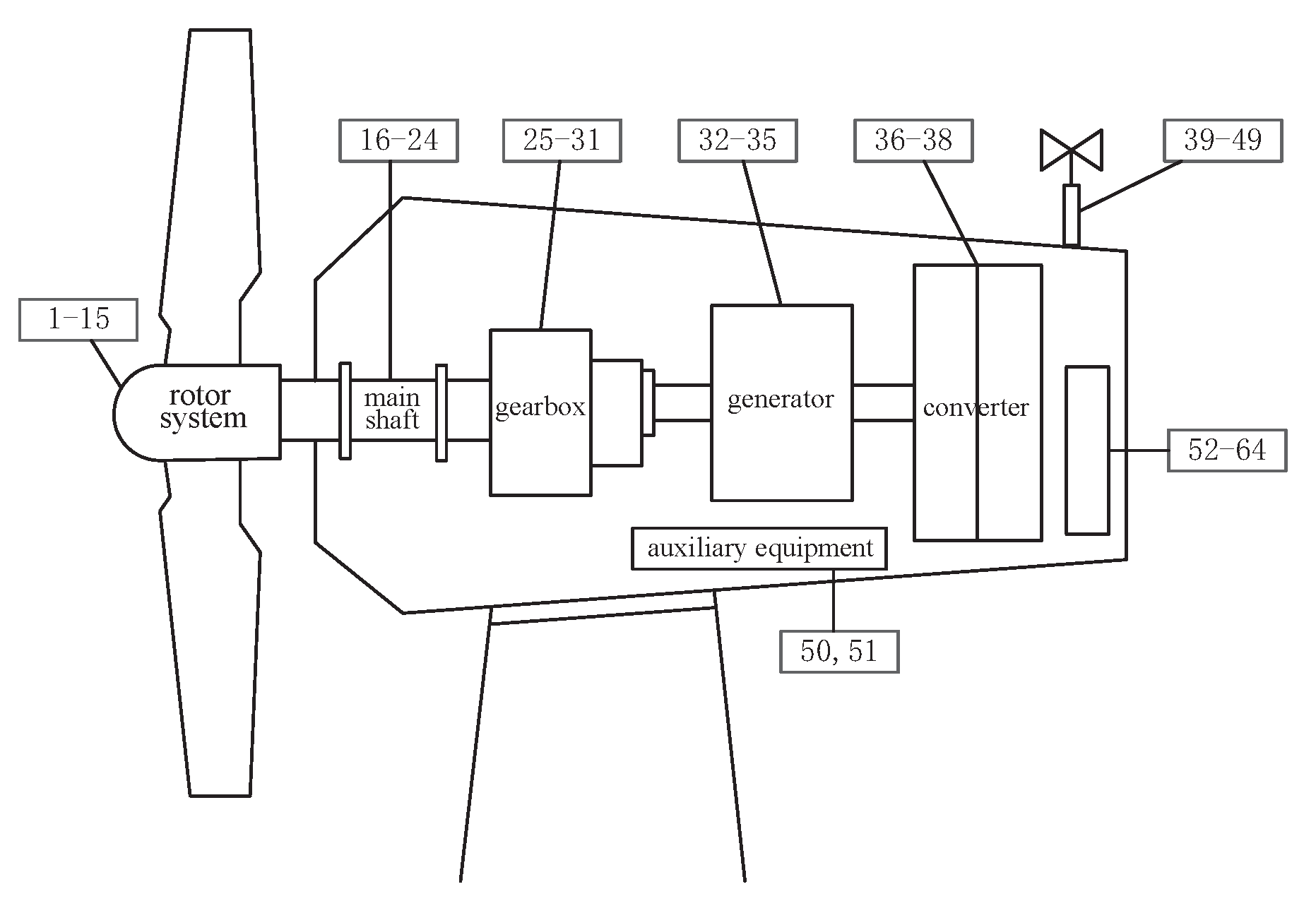
The experiment data are collected from a wind farm in the south of China. There are 33 WTs in the wind farm and the WT 8 was selected for research. Figure 7 shows the sensor structure of WT. The SCADA data collected at an interval of 10 minutes are used in experiments. The data in this WF are well-collected, with a complete record of anomaly. Figure 8 shows image of the wind farm. Table 1 shows the parameters of WTs.

Figure 7. Sensor structure of WT.

Figure 8. Image of the wind farm.

Table 1. Parameters of WTs.

No.	Parameter	Unit	No.	Parameter	Unit
1	Temp. of hub	${}^{\circ }$C	33	Temp. of generator output shaft	${}^{\circ }$C
2	Temp. of generator of blade 1	${}^{\circ }$C	34	Temp. of generator stator winding	${}^{\circ }$C
3	Temp. of generator of blade 2	${}^{\circ }$C	35	Speed of the generator	rpm
4	Temp. of generator of blade 3	${}^{\circ }$C	36	Ambient temperature of the converter	${}^{\circ }$C
5	Current of generator of blade 1	A	37	Measured torque of the converter	Nm
6	Current of generator of blade 2	A	38	Measured speed of the converter	rpm
7	Current of generator of blade 3	A	39	Wind direction
8	Function code		40	Absolute wind direction
9	Value of the encoder of blade 1A		41	Average wind direction of 1 s
10	Value of the encoder of blade 2A		42	Average wind direction of 1 min
11	Value of the encoder of blade 3A		43	Average wind direction of 10 min
12	Value of the encoder of blade 1B		44	Average wind velocity	m/s
13	Value of the encoder of blade 2B		45	Maximum wind velocity	m/s
14	Value of the encoder of blade 3B		46	Minimum wind speed	m/s
15	Angle of the cable	${}^{\circ }$	47	Average wind speed of 1 s	m/s
16	Temp. of the main bearing	${}^{\circ }$C	48	Average wind speed of 1 min	m/s
17	Pressure of the hydraulic system	bar	49	Average wind speed of 10 min	m/s
18	Speed of variable pitch for shaft 1	rpm	50	Ambient temperature	${}^{\circ }$C
19	Speed of variable pitch for shaft 2	rpm	51	Temp. of the cabin	${}^{\circ }$C
20	Speed of variable pitch for shaft 3	rpm	52	Frequency of power system	HZ
21	Vibration on x direction of node 100	g	53	Active power	kW
22	Vibration on y direction of node 100	g	54	Reactive power	kW
23	Vibration on x direction of node 101	g	55	Voltage of phase A	V
24	Vibration on y direction of node 101	g	56	Voltage of phase B	V
25	Speed of the gearbox	rpm	57	Voltage of phase C	V
26	Temp. of gearbox oil	${}^{\circ }$C	58	Current of phase A	A
27	Temp. of gearbox input shaft	${}^{\circ }$C	59	Current of phase B	A
28	Inlet temperature of the gearbox oil	${}^{\circ }$C	60	Current of phase C	A
29	Temp. of gearbox output shaft	${}^{\circ }$C	61	Average power of 1 s	kW
30	Pressure of gearbox oil pump	bar	62	Average power of 1 min	kW
31	Inlet pressure of the gearbox oil	bar	63	Average power of 10 min	kW
32	Temp. of generator input shaft	${}^{\circ }$C	64	Power factor

5.2. Model Parameters Setting

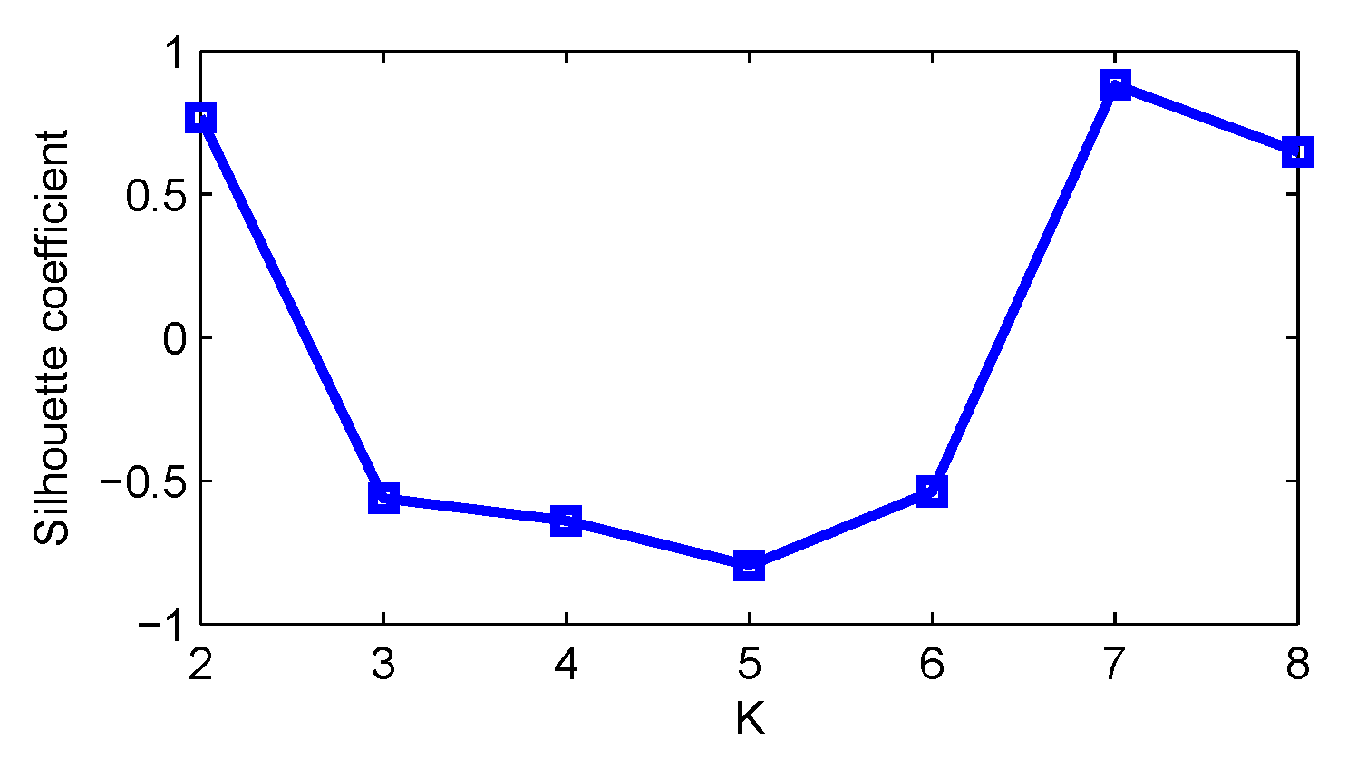
K-means clustering. There are 64 attributes in Table 1, and attributes are divided into eight categories according to the formula $k_{max}\le \sqrt{64}$. After normalization and clustering, the relation between cluster number K and SC is shown in Table 2 and Figure 9. The effect of SC (0.8814) is optimal when K = 7. Therefore, the attributes are divided into seven categories.

Table 2. Numerical relationship of SC and K.

K	SC
2	0.7699
3	−0.5612
4	−0.6385
5	0.7954
6	−0.5370
7	0.8814
8	0.6953

Figure 9. Curve of SC and K.

t-SNE dimension reduction. The attribute dimension is not less than 3, so the obtained attribute is 3 dimensions after dimension reduction. After a lot of training, the parameters setting of each class are shown in Table 3. Through the data preprocessing, the new attribute is X = 21 dimensions, and is used to input into deep neural network.

Table 3. t-SNE parameters setting of each class.

	1	2	3	4	5	6	7
Perp	100	50	40	30	25	40	40
T	3000	2000	500	1000	1000	1200	1500

deep neural network model. Each input image is normalized to 21 × 21 in this experiment, other settings as shown in Table 4. The number of second-level convolution kernels is obtained through multiple training. The specific training parameters of the optimal model obtained through multiple experiments are shown in Table 5.

Table 4. Architecture of Deep Neural Network.

The first convolution layer	6 kernels of size 6 × 6
Output the feature map	6 maps of size 16 × 16
The first pool layer	2 × 2
Output the feature map	6 maps of size 8 × 8
The second convolution layer	12 kernels of size 3 × 3
The second pool layer	2 × 2
Output the feature map	12 maps of size 3 × 3

Table 5. Training parameter settings.

learning rate:alpha	1
The number of samples in batch training:batchsize	10
Iteration number:numepochs	2

Test example. According to the settings in Table 4 and Table 5, the test example is shown in Figure 10. The normalized WT images are represented by C1, S1, C2, and S2.

Figure 10. Output process of each layer.

5.3. Cases Analysis

Experimental data includes 20,000 training images and 100 test images. The ratio of normal data to abnormal data is 1:1. The size of the input picture is 21 × 21. The following three cases were conducted: (1) Single anomaly detection of 1st attribute. (2) Multi-anomalies detection of 6th attribute. (3) Multi-anomalies detection of multi-attributes.

5.3.1. Cases 1: Single Anomaly Detection of 1st Attribute

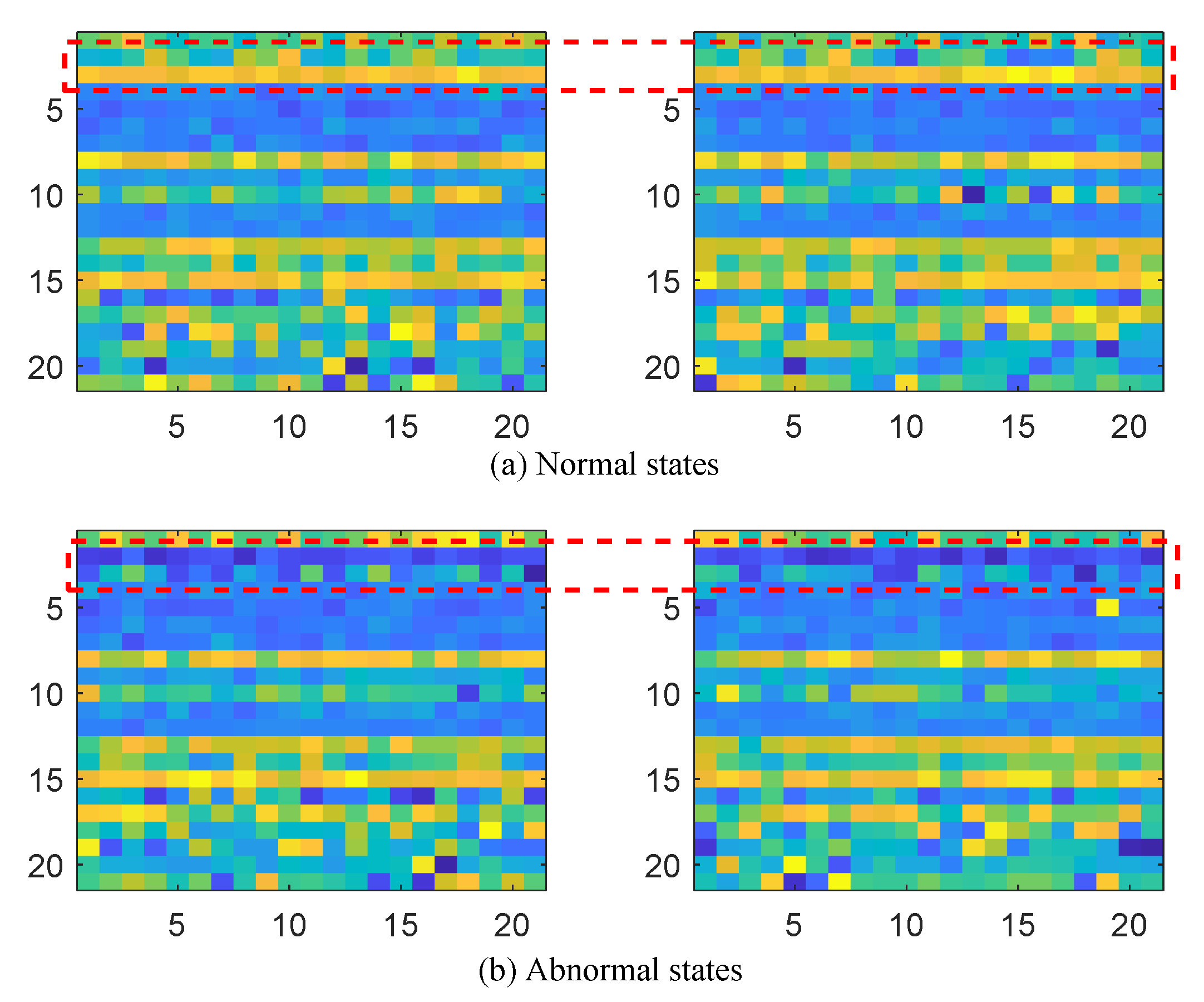
The anomaly is that the temperature of gearbox output shaft is overheating. Figure 11 is comparison of the normal and abnormal images. The size of each image is 21 × 21 and every three rows in the image belongs a category. Figure 11a are normal states at different times. Figure 11b are abnormal states at different times. The first three rows of the image represent the 1st attribute.

Figure 11. Comparison of normal and abnormal.

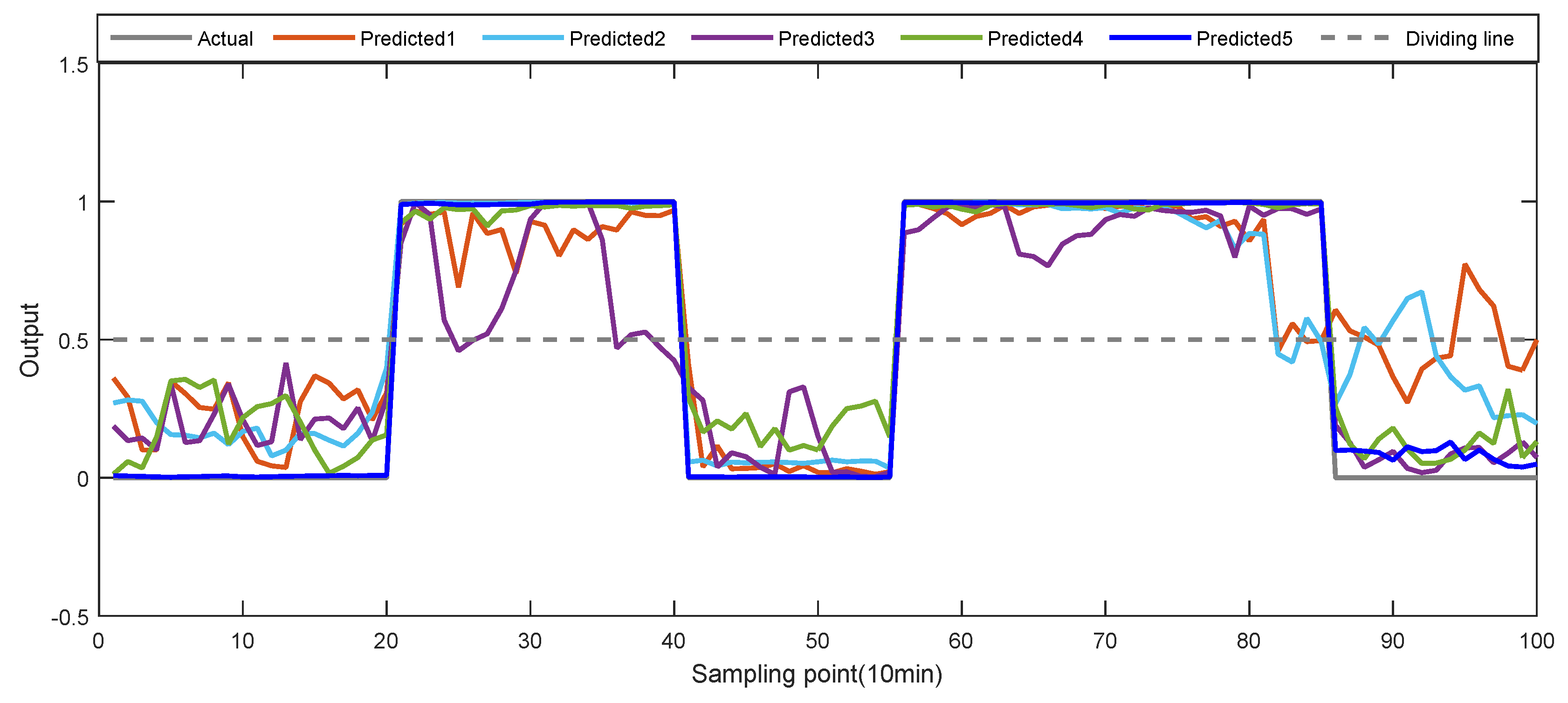
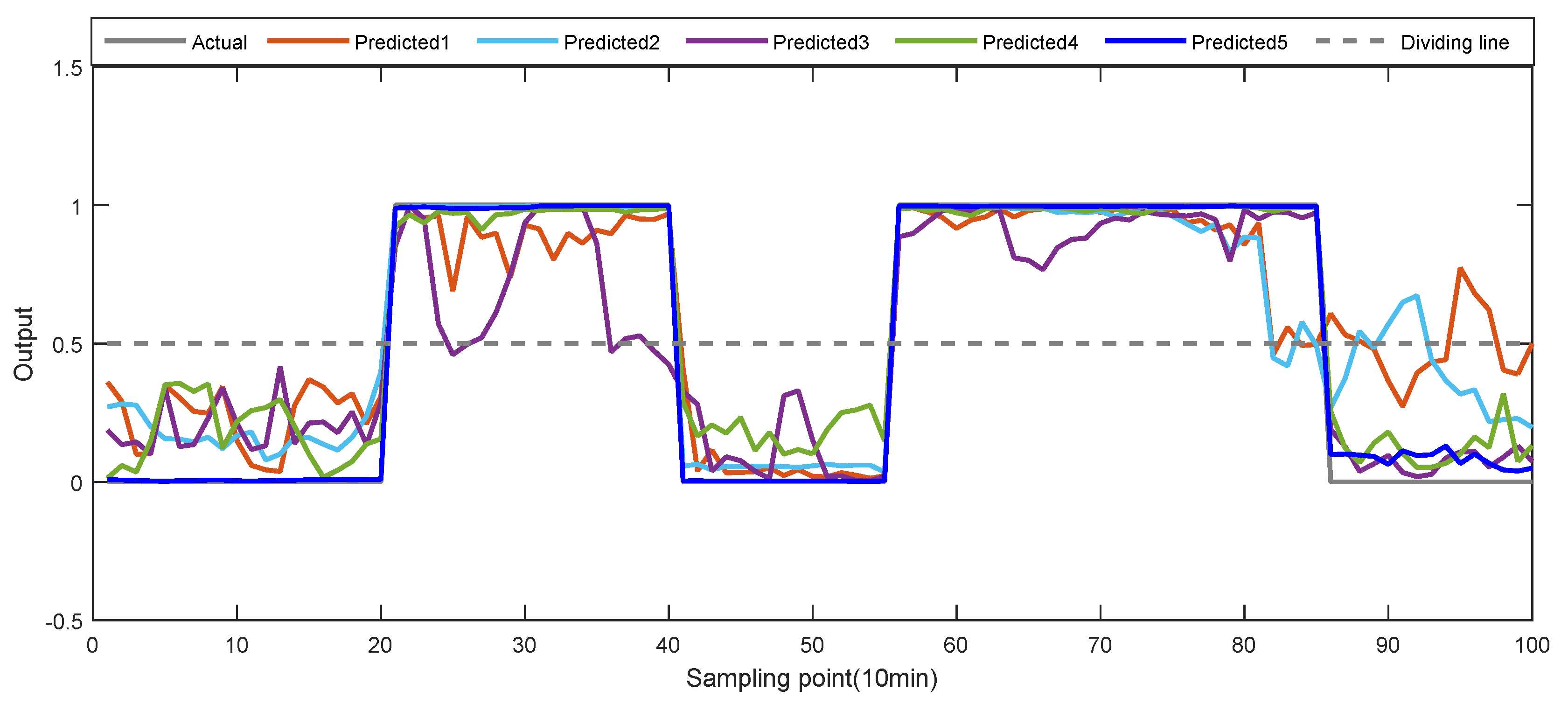
The model based on deep neural network is used to estimate the state of WT. The test samples are randomly selected. Figure 12 shows the five test experiments. The experiment including 48 normal data and 52 abnormal data. Gray lines represent actual values, five other colored lines represent predicted values. If the output value is less than 0.5, the state is 0 (abnormal), otherwise the state is 1 (normal). The result is shown in Table 6.

Figure 12. Output values of five test experiments.

Table 6. Results of five test experiments.

	1	2	3	4	5	SUM
TA	46	45	44	47	45	227
FA	6	7	8	5	7	33
TH	44	43	45	40	46	218
FH	4	5	3	8	2	22

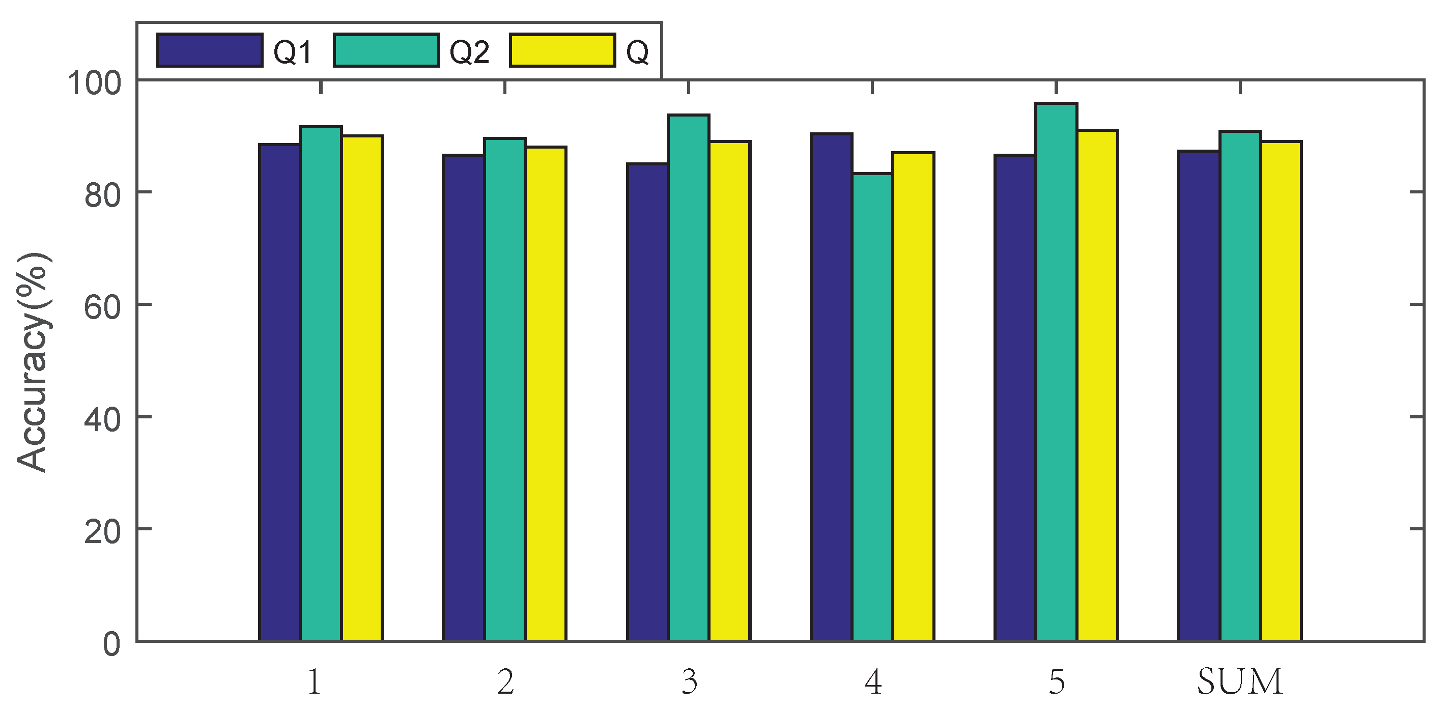
Table 7 and Figure 13 show the accuracy of Q1, Q2, Q. From the experiment results, it can be concluded that the proposed method is effective in single anomaly detection.

Table 7. Accuracy of five test experiments.

	1	2	3	4	5	Average
Q1	88%	87%	85%	90%	87%	87.4%
Q2	92%	90%	94%	83%	96%	91%
Q	90%	88%	89%	87%	91%	89%

Figure 13. Accuracy of Q1, Q2, Q.

5.3.2. Cases 2: Multi-Anomalies Detection of 6th Attribute

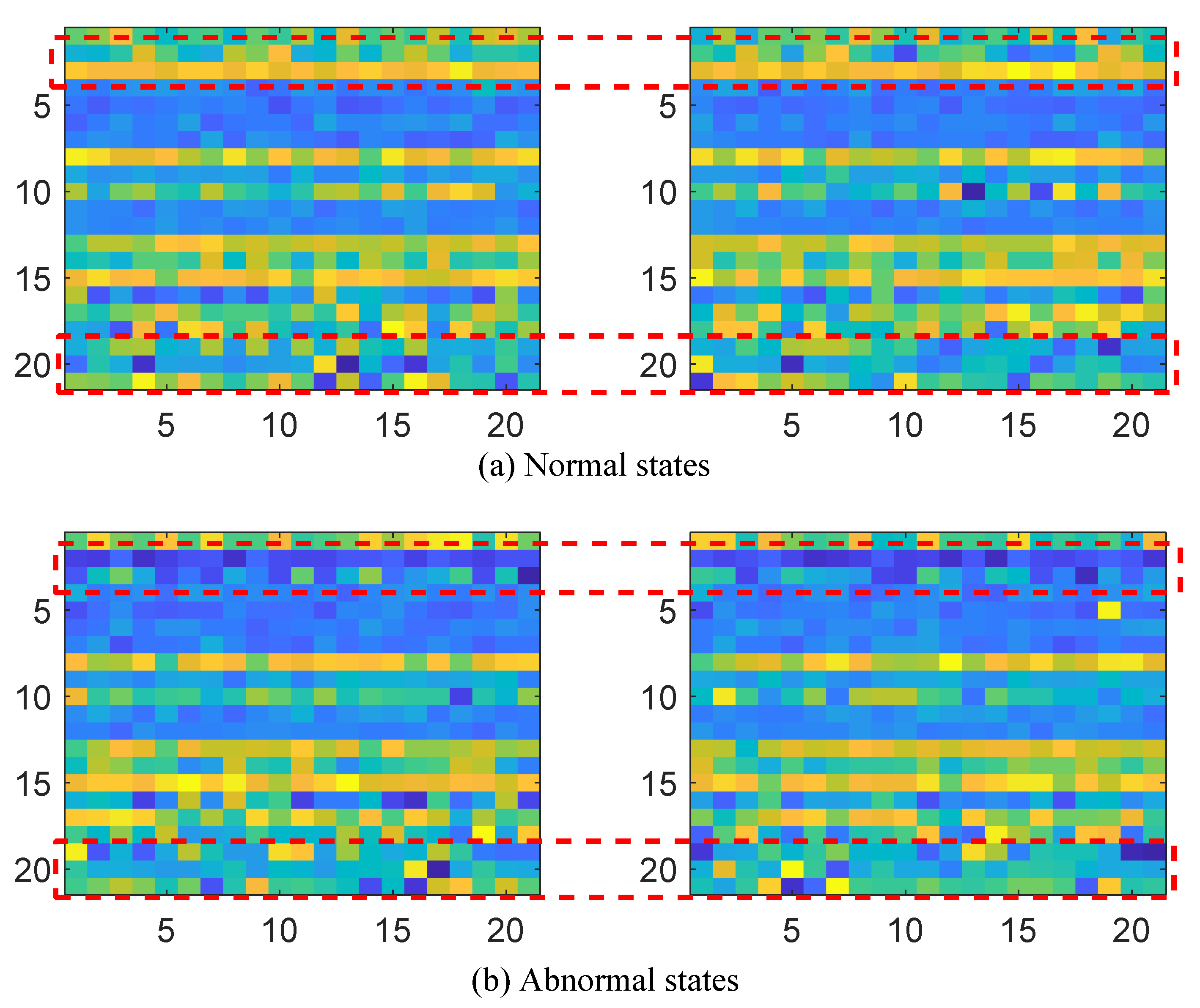
The anomalies are the speed of the generator is reduced and the speed of gearbox is reduced. Figure 14 is comparison of the normal and abnormal images. Figure 14a are normal states at different times. Figure 14b are abnormal states at different times. Rows 16 to 18 indicate the 6th attribute.

Figure 14. Comparison of normal and abnormal.

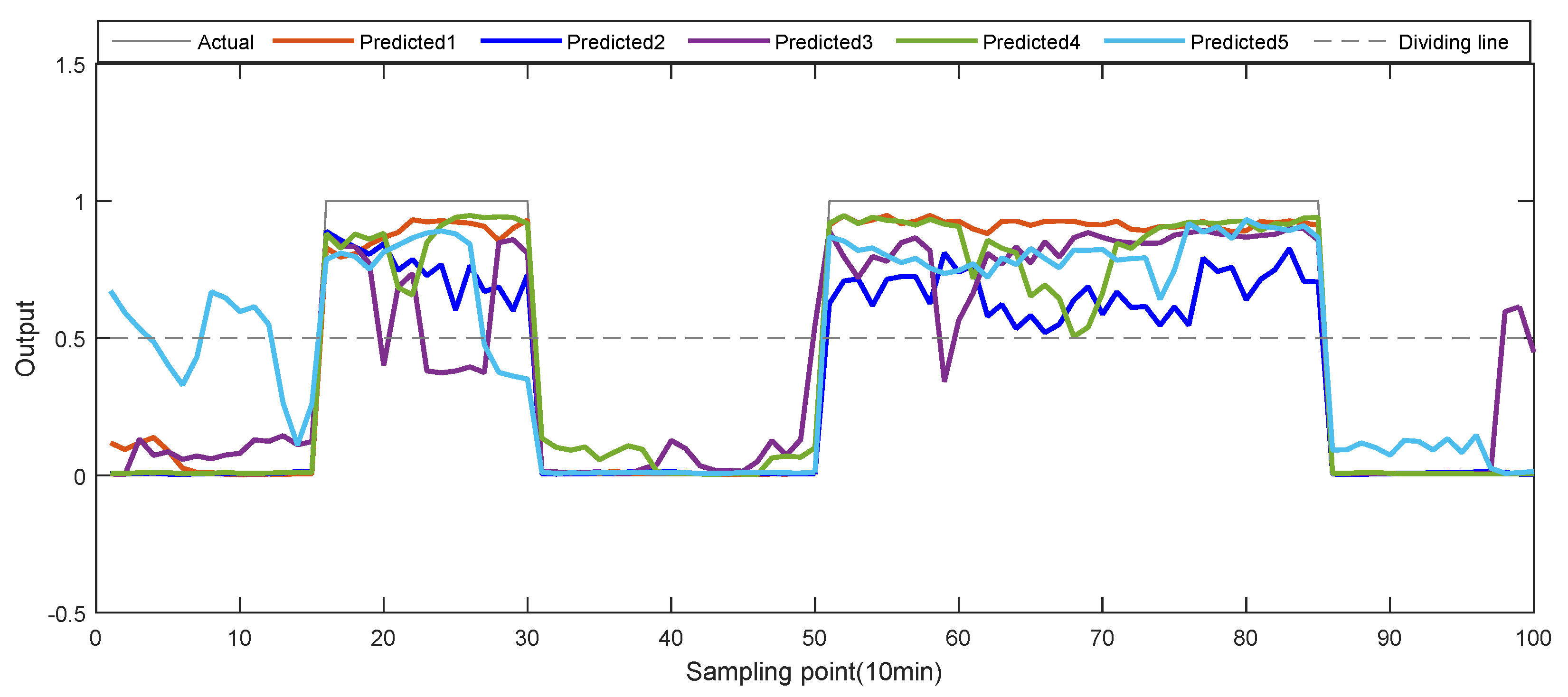
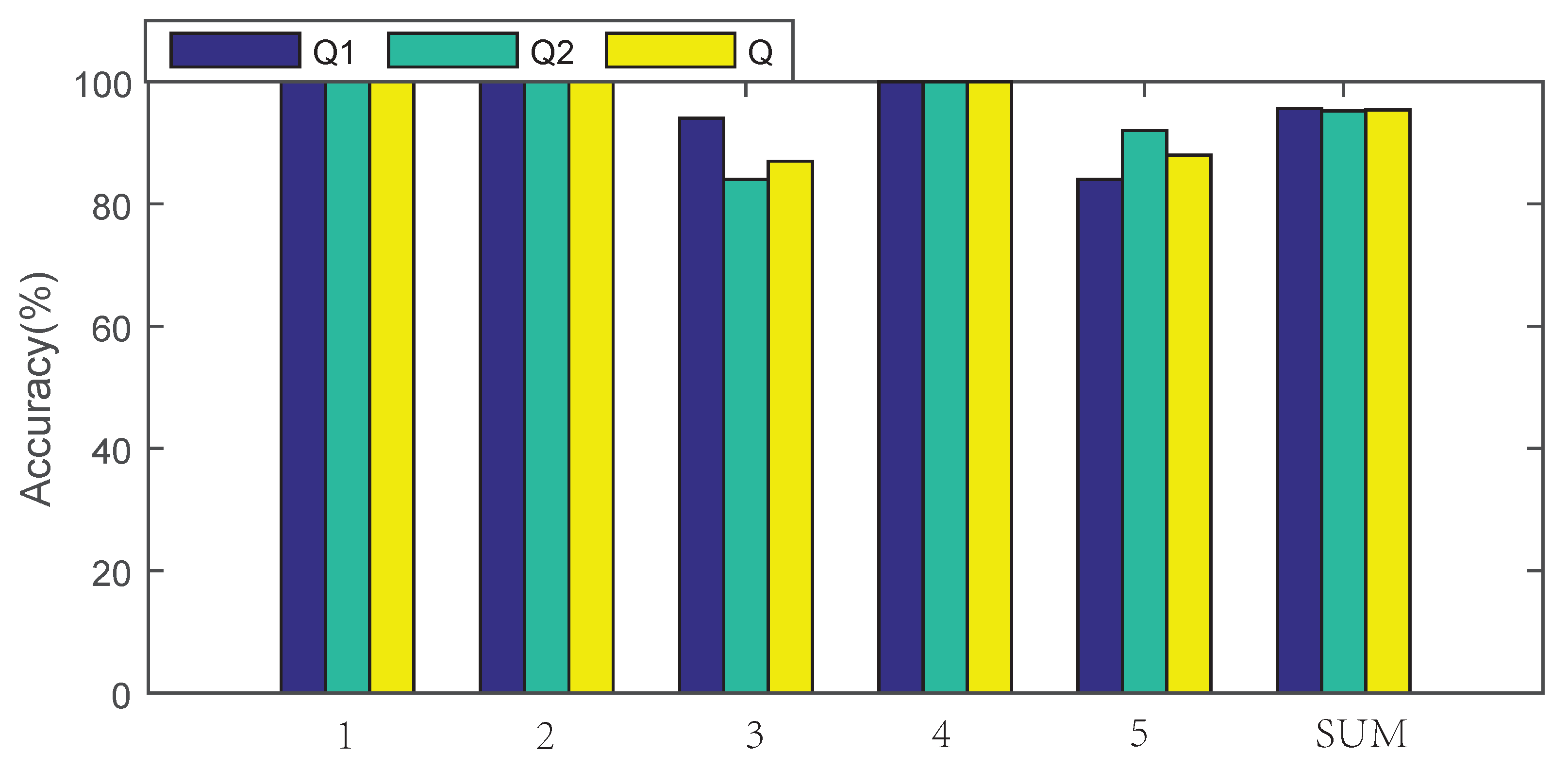
Figure 15 shows the five test experiments. The experiment including 50 normal data and 50 abnormal data. Table 8 shows five results of test experiments. Table 9 and Figure 16 show the accuracy of Q1, Q2, Q. The average accuracy is 95.4%, which is higher than case1. From the experiment results, it can be concluded that the proposed method is effective in multi-anomaly detection.

Figure 15. Output values of five test experiments.

Table 8. Results of five test experiments.

	1	2	3	4	5	SUM
TA	50	50	47	50	42	239
FA	0	0	3	0	8	11
TH	50	50	42	50	46	238
FH	0	0	8	0	4	12

Table 9. Accuracy of five test experiments.

	1	2	3	4	5	Average
Q1	100%	100%	94%	100%	84%	95.6%
Q2	100%	100%	84%	100%	92%	95.2%
Q	100%	100%	89%	100%	88%	95.4%

Figure 16. Accuracy of Q1, Q2, Q.

5.3.3. Cases 3: Multi-Anomalies Detection of Multi-Attributes

The anomalies are the temperature of gearbox oil and temperature of gearbox input shaft increase both in the 1st and 7th attributes. The attributes and anomalies are selected randomly. Figure 17 is comparison of the normal and abnormal images. Figure 17a are normal states at different times. Figure 17b are abnormal states at different times. Rows 1 to 3 indicate the 1st attribute and rows 19 to 21 indicate the 7th attribute.

Figure 17. Comparison of normal and abnormal.

Figure 18 shows the five test experiments. The experiment including 50 normal data and 50 abnormal data. Table 10 shows five results of accuracy. The average accuracy of normal state is 95.6%, the average accuracy of abnormal state is 96%. Therefore, the average accuracy of the five test experiments is 95.8%, which is higher than case1. From the experiment results, it can be concluded that the proposed method is effective in multi-anomalies detection of multi-attributes.

Figure 18. Output values of five test experiments.

Table 10. Accuracy of five test experiments.

	1	2	3	4	5	Average
Q1	88%	92%	100%	100%	100%	96%
Q2	94%	94%	90%	100%	100%	95.6%
Q	91%	93%	90%	100%	100%	95.8%

To further verify the effectiveness of the proposed method, other two methods are adopted to make the comparison: (1) BPNN method, (2) SVM method. The experiment results shown in Table 11. It can be concluded that the average accuracy of proposed method is 95.8%, and it has the best performance in the experiment.

Table 11. Comparison results of three methods.

Method	Q1	Q2	Q
BPNN	81.2%	84.8%	83%
SVM	80.4%	83.6%	82%
The proposed method	96%	95.6%	95.8%

6. Conclusions

In this paper, a wind turbine anomaly detection method based on SCADA data mining is proposed. Firstly, WT attributes collected from the SCADA system are clustered by k-means, and then the method of dimension reduction within class based on t-SNE is proposed. Finally, the detection model is trained and the abnormal or normal state is detected by the classification result 0 or 1 respectively. Three cases are conducted in this paper to demonstrate the effectiveness of the proposed method. The results show that the proposed method has good performance in three cases: (1) single anomaly detection of 1st attribute, (2) multi-anomalies detection of 6th attribute, (3) multi-anomalies detection of multi-attributes. In the future, we will continue our research on anomaly detection, and developing more effective deep learning methods to predict anomalies before they occur.

References

1. Amirat, Y.; Benbouzid, M.E.H.; Al-Ahmar, E.; Bensa, B.; Turri, S. A brief status on condition monitoring and fault diagnosis in wind energy conversion systems. Renew. Sustain. Energy Rev. 2009, 13, 2629–2636. [Google Scholar] [CrossRef]
2. Márquez, F.P.G.; Tobias, A.M.; Pérez, J.M.P.; Papaelias, M. Condition monitoring of wind turbines: Techniques and methods. Renew. Energy 2012, 46, 169–178. [Google Scholar] [CrossRef]
3. Qian, P.; Zhang, D.; Tian, X.; Si, Y.; Li, L. A novel wind turbine condition monitoring method based on cloud computing. Renew. Energy 2019, 135, 390–398. [Google Scholar] [CrossRef]
4. Zhang, F.; Wen, Z.; Liu, D.; Jiao, J.; Wan, H.; Zeng, B. Calculation and Analysis of Wind Turbine Health Monitoring Indicators Based on the Relationships with SCADA Data. Appl. Sci. 2020, 10, 407. [Google Scholar] [CrossRef]
5. Lutz, M.A.; Vogt, S.; Berkhout, V.; Faulstich, S.; Dienst, S.; Steinmetz, U.; Gück, C.; Ortega, A. Evaluation of Anomaly Detection of an Autoencoder Based on Maintenace Information and Scada-Data. Energies 2020, 13, 1063. [Google Scholar] [CrossRef]
6. Davide, A.; Francesco, C.; Francesco, N. Wind Turbine Generator Slip Ring Damage Detection through Temperature Data Analysis. Diagnostyka 2019, 20, 3–9. [Google Scholar]
7. Tang, M.; Chen, W.; Zhao, Q.; Wu, H.; Long, W.; Huang, B.; Liao, L.; Zhang, K. Development of an SVR Model for the Fault Diagnosis of Large-Scale Doubly-Fed Wind Turbines Using SCADA Data. Energies 2019, 12, 3396. [Google Scholar] [CrossRef]
8. Shao, H.; Gao, Z.; Liu, X.; Busawon, K. Parameter-varying modelling and fault reconstruction for wind turbine systems. Renew. Energy 2018, 116, 145–152. [Google Scholar]
9. Hwang, I.; Kim, S.; Kim, Y.; Seah, C.E. A survey of fault detection, isolation, and reconfiguration methods. IEEE Trans. Control Syst. Technol. 2009, 18, 636–653. [Google Scholar] [CrossRef]
10. Hameed, Z.; Hong, Y.S.; Cho, Y.M.; Ahn, S.H.; Song, C.K. Condition monitoring and fault detection of wind turbines and related algorithms: A review. Renew. Sustain. Energy Rev. 2009, 13, 1–39. [Google Scholar] [CrossRef]
11. Simani, S.; Alvisi, S.; Venturini, M. Data-Driven Control Techniques for Renewable Energy Conversion Systems: Wind Turbine and Hydroelectric Plants. Electronics 2019, 8, 237. [Google Scholar] [CrossRef]
12. Schlechtingen, M.; Santos, I.F. Wind turbine condition monitoring based on SCADA data using normal behavior models. Part 2: Application examples. Appl. Soft Comput. 2014, 14, 447–460. [Google Scholar] [CrossRef]
13. Zhang, Y.; Li, M.; Dong, Z.Y.; Meng, K. A probabilistic anomaly detection approach for data-driven wind turbine condition monitoring. Int. J. Electr. Power Energy Syst. 2019, 5, 149–158. [Google Scholar] [CrossRef]
14. Cui, Y.; Bangalore, P.; Tjernberg, L.B. An Anomaly Detection Approach Based on Machine Learning and SCADA Data for Condition Monitoring of Wind Turbines. In Proceedings of the 2018 IEEE International Conference on Probabilistic Methods Applied to Power Systems (PMAPS), Boise, ID, USA, 24–28 June 2018. [Google Scholar]
15. Kusiak, A.; Verma, A. A data-mining approach to monitoring wind turbines. IEEE Trans. Sustain. Energy 2011, 3, 150–157. [Google Scholar] [CrossRef]
16. Kusiak, A.; Verma, A. A data-driven approach for monitoring blade pitch faults in wind turbines. IEEE Trans. Sustain. Energy 2010, 2, 87–96. [Google Scholar] [CrossRef]
17. Aghenta, L.; Iqbal, T. Low-Cost, Open Source IoT-Based SCADA System Design Using Thinger. IO and ESP32 Thing. Electronics 2019, 8, 822. [Google Scholar] [CrossRef]
18. González, I.; Calderón, A.J. Integration of open source hardware Arduino platform in automation systems applied to Smart Grids/Micro-Grids. Sustain. Energy Technol. Assess. 2019, 36, 100557. [Google Scholar] [CrossRef]
19. Vargas-Salgado, C.; Aguila-Leon, J.; Chiñas-Palacios, C.; Hurtado-Perez, P. Low-cost web-based Supervisory Control and Data Acquisition system for a microgrid testbed: A case study in design and implementation for academic and research applications. Heliyon 2019, 5, e02474. [Google Scholar] [CrossRef]
20. Salgado-Plasencia, E.; Carrillo-Serrano, R.V.; Rivas-Araiza, E.A.; Toledano-Ayala, M. SCADA-Based Heliostat Control System with a Fuzzy Logic Controller for the Heliostat Orientation. Appl. Sci. 2019, 9, 2966. [Google Scholar] [CrossRef]
21. Tautz-Weinert, J.; Watson, S.J. Using SCADA data for wind turbine condition monitoring—A review. IET Renew. Power Gener. 2016, 11, 382–394. [Google Scholar] [CrossRef]
22. Larios, D.F.; Personal, E.; Parejo, A.; García, S.; García, A.; Leon, C. Operational Simulation Environment for SCADA Integration of Renewable Resources. Energies 2020, 13, 1333. [Google Scholar] [CrossRef]
23. Sun, P.; Li, J.; Wang, C.; Lei, X. A generalized model for wind turbine anomaly identification based on SCADA data. Appl. Energy 2016, 168, 550–567. [Google Scholar] [CrossRef]
24. Santos, P.; Villa, L.F.; Reñones, A.; Bustillo, A.; Maudes, J. An SVM-based solution for fault detection in wind turbines. Sensors 2015, 15, 5627–5648. [Google Scholar] [CrossRef] [PubMed]
25. Wang, L.; Zhang, Z.; Long, H.; Xu, J.; Liu, R. Wind turbine gearbox failure identification with deep neural networks. IEEE Trans. Ind. Inf. 2016, 13, 1360–1368. [Google Scholar] [CrossRef]
26. Shanlin, Y.; Yongsen, L.; Xiaoxuan, H. Study on the value optimization of k-means algorithm. Syst. Eng. Theory Pract. 2006, 2, 97–101. [Google Scholar]
27. Fukushima, K. Neocognitron: A self-organizing neural network model for a mechanism of pattern recognition unaffected by shift in position. Biol. Cybern. 1980, 36, 193–202. [Google Scholar] [CrossRef]
28. Lawrence, S.; Giles, C.L.; Tsoi, A.C.; Back, A.D. Face recognition: A convolutional neural-network approach. IEEE Trans. Neural Netw. 1997, 8, 98–113. [Google Scholar] [CrossRef]
29. Chen, Y.; Jiang, H.; Li, C.; Jia, X.; Ghamisi, P. Deep feature extraction and classification of hyperspectral images based on convolutional neural networks. IEEE Trans. Geosci. Remote Sens. 2016, 54, 6232–6251. [Google Scholar] [CrossRef]
30. He, K.; Zhang, X.; Ren, S.; Sun, J. Spatial pyramid pooling in deep convolutional networks for visual recognition. IEEE Trans. Pattern Anal. Mach. Intell. 2015, 37, 1904–1916. [Google Scholar] [CrossRef]
31. Cun, Y.L.; Bengio, Y. Word-level training of a handwritten word recognizer based on convolutional neural networks. In Proceedings of the 12th IAPR International Conference on Pattern Recognition, Jerusalem, Israel, 9–13 October 1994; pp. 88–92. [Google Scholar]
32. Nair, V.; Hinton, G. Rectified linear units improve restricted boltzmann Machines. In Proceedings of the 27th International Conference on International Conference on Machine Learning, Haifa, Israel, 21–24 June 2010; pp. 807–814. [Google Scholar]
33. LeCun, Y.; Ranzato, M. Deep learning tutorial. In Proceedings of the International Conference on Machine Learning (ICML13), Atlanta, GA, USA, 16–21 June 2013. [Google Scholar]
34. Glorot, X.; Bordes, A.; Bengio, Y. Deep sparse rectiler neural networks. In Proceedings of the Fourteenth International Conference on Artificial Intelligence and Statistics, Fort Lauderdale, FL, USA, 11–13 April 2011; pp. 315–323. [Google Scholar]
Article Metrics
Citations
Article Access Statistics
Multiple requests from the same IP address are counted as one view.