Article

Goal-Oriented Obstacle Avoidance with Deep Reinforcement Learning in Continuous Action Space

1
Department of Intelligent Robot Engineering, Hanyang University, Seoul 04763, Korea
2
Department of Electronics and Computer Engineering, Hanyang University, Seoul 04763, Korea
*
Author to whom correspondence should be addressed.
Electronics 2020, 9(3), 411; https://doi.org/10.3390/electronics9030411
Submission received: 20 January 2020 / Revised: 24 February 2020 / Accepted: 26 February 2020 / Published: 28 February 2020
(This article belongs to the Section Artificial Intelligence)

Abstract

:
In this paper, we propose a goal-oriented obstacle avoidance navigation system based on deep reinforcement learning that uses depth information in scenes, as well as goal position in polar coordinates as state inputs. The control signals for robot motion are output in a continuous action space. We devise a deep deterministic policy gradient network with the inclusion of depth-wise separable convolution layers to process the large amounts of sequential depth image information. The goal-oriented obstacle avoidance navigation is performed without prior knowledge of the environment or a map. We show that through the proposed deep reinforcement learning network, a goal-oriented collision avoidance model can be trained end-to-end without manual tuning or supervision by a human operator. We train our model in a simulation, and the resulting network is directly transferred to other environments. Experiments show the capability of the trained network to navigate safely around obstacles and arrive at the designated goal positions in the simulation, as well as in the real world. The proposed method exhibits higher reliability than the compared approaches when navigating around obstacles with complex shapes. The experiments show that the approach is capable of avoiding not only static, but also dynamic obstacles.

1. Introduction

With the recent advances in computing and sensor technologies, the prevalence of robotic devices in our everyday lives is increasing. Currently, robots are freely interacting with physical environments and navigating in them. However, realizing this in varying real-world situations can still be a daunting task. In unpredictable surroundings, such fundamental capabilities as mobile robot navigation require much attention. For mobile robots to navigate successfully in real-world environments, they need not only the ability to navigate to a goal, but also avoid collisions in a safe manner. Generally, a path planner can be employed to find a clear path in the free space of the environment. However, in varying or unknown spaces, it is hard to generate such a path. Unless the work environment is fully described, it is hard to guarantee that the generated path will not lead to a collision. Keeping track and considering all the changes in the planning stage of navigation is unfeasible. Therefore, robot navigation must include a way to detect and avoid obstacles with only local information in space and time.
Multiple types of sensors can be used to recognize occupancy in the environment such as laser scanners, sonars, depth cameras, or bumps. By using sensory data, a robot can navigate towards a clear path. Such behavior can be programmed into the navigation system. For example, when an object is at a certain predetermined distance from the robot, an action can be programmed to avoid it. However, it can be very difficult and time consuming to predict all possible situations that the robot may encounter. Recent advances in deep reinforcement learning have shown the ability to solve increasingly more complex tasks. These methods have been successfully adopted in a wide variety of fields and have been applied to robot navigation. This has made it possible to exclude the necessity of human supervision and environment-dependent manual engineering of robots. For this method to be viable, the robot needs to gather a large variety of experiences, which might be costly if performed in the real world. Owing to the generalization ability of deep learning models, it is possible to learn in a simulated environment and apply the trained network to the real world. For this reason, the network needs to have as much information about the surroundings as possible, while still outputting navigation commands in a timely manner. This creates an issue of implementing navigation systems with a large input space, such as images, which require significant computing power to facilitate the network parameters. To reduce the computing burden of standard convolution for image processing, depth-wise separable convolution was established in [1]. It has achieved comparable results with significantly reduced multiply-accumulation operations and parameters [2,3]. This allows significant amounts of image data to be used in real-time robotic applications with limited computing resources. Yet, to obtain goal-oriented navigation, the processed image data still need to be combined with the goal position information.
In this paper, we set out to overcome these challenges and propose a navigation system that learns in a simulated environment how to avoid obstacles in collaboration with goal-oriented navigation. To achieve this purpose, we use depth images and the estimated position with respect to the goal of the robot as inputs to the network. We aim to improve upon the existing approaches, have the capability of processing input signals of higher complexity, and solve the issues associated with it. The main contributions of this paper can be itemized as follows:
  • Creation of a convolutional deep deterministic policy gradient network for tackling a large amount of input data.
  • Development of a deep deterministic policy gradient network with mixed inputs for goal-oriented collision avoidance.
  • Transfer of a network, learned in a simulation, to the real environment for map-less vector navigation with depth image inputs.
The remainder of this paper is organized as follows. In Section 2, the related works are reviewed. The proposed network is described in Section 3. Training of the network is explained in Section 4, followed by experimental results given in Section 5. Finally, a summary and discussion are presented in Section 6.

2. Related Works

In an ideal situation, the robot would be fully aware of its surroundings and move in a completely known environment. In such cases, a multitude of possible algorithms exist that can plan and execute the robot motion to the goal. If all of the obstacles are known, a path planner can be employed to set a path for a robot to follow. Algorithms such as A*, RRT*, and their extensions [4,5,6,7] are quick and easy ways of obtaining a path. To obtain better or constrained paths, heuristic methods are combined with optimization algorithms [8,9,10,11]. Here, optimization algorithms, such as genetic algorithm, simulated annealing, and others, are introduced during the planning and post-processing phases to obtain the optimal path. However, if they encounter an obstacle, the planning needs to be performed again. Reactive re-planing can be performed with the D* algorithm and its extensions [12,13], but still, the map of the environment should be known beforehand or the algorithms work with the assumption that the previously known free space holds no obstacles. Obtaining a full map of the environment often can be unfeasible or even impossible, especially if the robot is deployed in a new, unknown environment. Therefore, fully planned approaches cannot always be implemented, and the obstacle avoidance strategy in unknown environments needs to be developed.
In an unknown or uncertain environment, obstacle avoidance is typically solved by using range sensors and applying predetermined logic [14]. The sensor input is used to detect the obstacles. Here, visual SLAM methods can be used to understand the environment and navigate the robot [15,16,17]. Segmentation can recognize traversable planes from a visual image or point cloud [18,19,20]. Laser, sonar, and other range sensors can detect obstacles and their shape to determine in which direction to move [14,21,22,23]. Especially, sensor readings from multiple robots through a centralized communications network are used [24]. When the surroundings have been mapped, the path planners can be updated based on set parameters for motion towards the goal. However, here, the collision avoidance is usually implemented by decoupling the object recognition and motion planning. First, an obstacle is detected, and then, the motion is selected based on policy. The policy needs to be described beforehand and based on the obstacle. It might not only be difficult to program an intelligent avoidance strategy, but also cause an issue when encountering previously unseen obstacles.
Currently, deep learning has shown great progress in dealing with large scale input data and directly producing finely-tuned policies in various applications, such as playing video games [25,26,27], stock market analysis [28,29,30], as well as various implementations in robotics [31]. Deep learning networks have been used in robotic applications to learn the navigation, as well as collision avoidance from the input signals [32,33,34,35,36]. Several applications have been developed that directly obtain motion policies from raw images [37,38,39]. Here, the motion policies are a direct result of the input image and do not require fine-tuning by an outside source. In [39], a dueling architecture-based Deep Double Q Network (D3QN) was used to obtain depth predictions from a monocular depth camera and perform collision avoidance. The network aims to avoid obstacles, but navigates without a specified goal position. Additionally, the D3QN algorithm outputs are in a discrete action space, which can result in rough navigation behaviors. In [40], the authors proposed a deep reinforcement learning model that separates the navigation towards a goal and the collision avoidance. The proposed two-stream Q network model learns the goal navigation and collision avoidance tasks separately, and the given actions are combined using an action scheduling method. The proposed approach uses a 360 laser range finder as the input and outputs actions in a discrete action space. Predetermined heuristics are used to decide the switching between navigation and obstacle avoidance actions. For the deep reinforcement learning to be capable of producing outputs in a continuous action space, the authors of [41] proposed a Deep Deterministic Policy Gradient (DDPG) network. This network was extended for map-less navigation purposes in [33] as an Asynchronous Deep Deterministic Policy Gradient (ADDPG) network. Here, measurements from a laser scanner in 10 directions and estimated robot location are used as the environmental information to navigate the robot towards a goal. A 180 laser sensor must be installed on the robot, and the state input considers only the current state of the robot. Laser sensor inputs are easily implementable in deep learning networks, especially if the number of inputs is reduced to minimize the number of learning parameters. However, they might not reflect a sophisticated scene in the environment since they generally produce information at a set height and have difficulties navigating around objects of certain shapes, as we show in Section 5.
Using deep reinforcement learning leads the network to tune its parameters based on the value function. However, without supervision, the network has to go through trial and error to explore and learn the best policy for the multitude of states it can encounter. This means that the training is difficult to perform in a real environment and tends to be done mostly in simulation. Several works [33,39,42,43] showed that deep learning networks are trainable in virtual environments and afterward transferable to the real world in robot applications. In this paper, we aim to create a goal-oriented collision avoidance navigation system that makes decisions on policies based directly on the sequential depth images and estimated goal location.

3. Deep Learning Network for Collision Avoidance in a Continuous Action Space

To tackle the problem of learning when and how to avoid obstacles from a depth image and goal location without a pre-existing map, we propose a Convolutional Deep Deterministic Policy Gradient (CDDPG) network. The CDDPG is Deep Deterministic Policy Gradient-based (DDPG) [41,44] network with depth-wise separable convolutional layers that are designed to deal with the large scale information of the depth images efficiently. DDPG networks are actor-critic networks that output an action in a continuous space.

3.1. Convolutional Deep Deterministic Policy Gradient

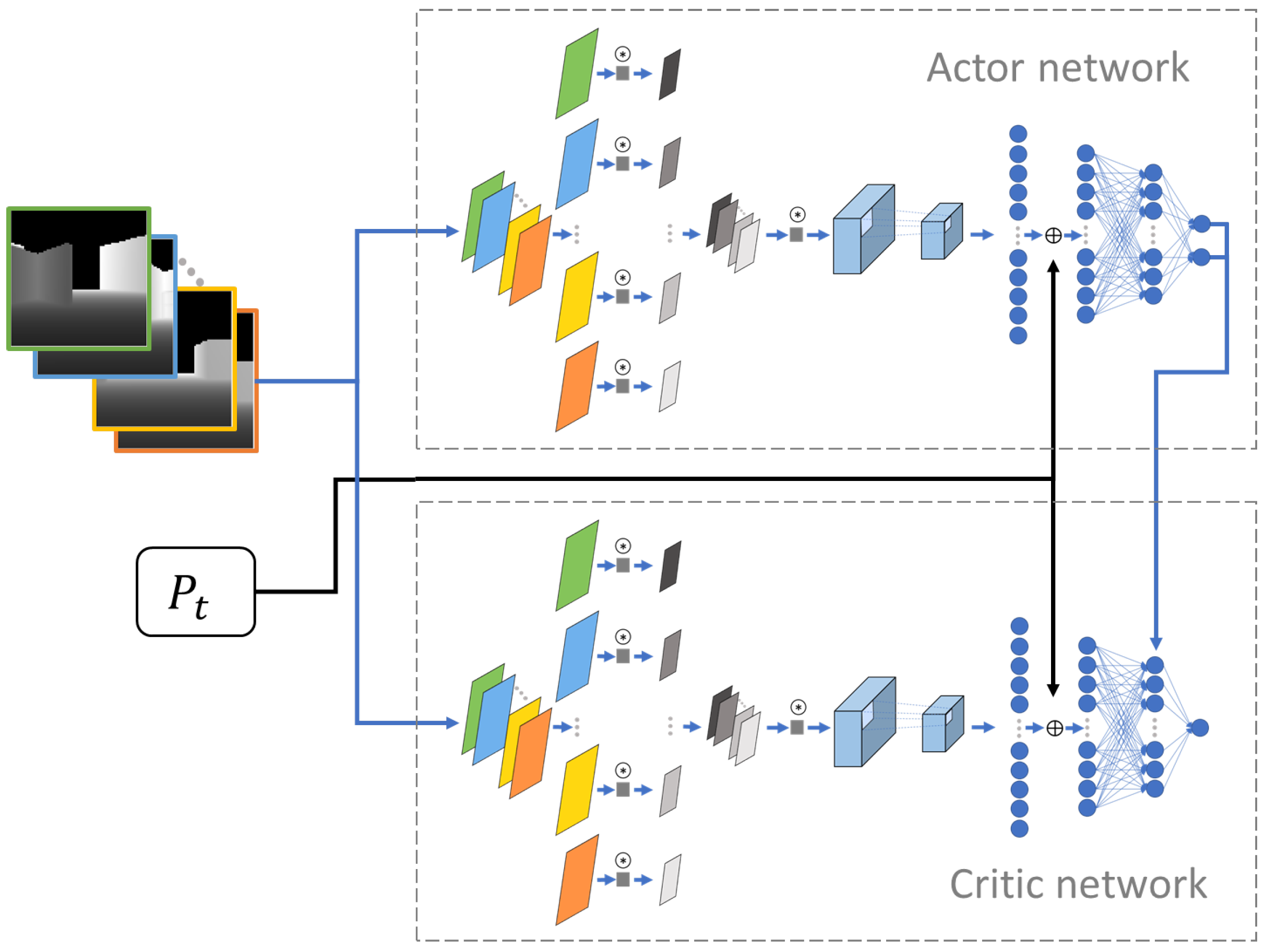
For effective goal-oriented obstacle avoidance from depth images in a continuous action space, we devised a DDPG-based network by implementing depth-wise separable convolutional layers. A DDPG-based network is an actor-critic type of network with similar structures of layer layouts for both parts, but with separate parameters. As the input of the actor network, we combined a stack of depth images with distance information to the goal, and the output was a set of real values representing angular velocity ω and linear velocity v, obtained from a continuous action space. The critic network takes the action produced by the actor, as well as the state as an input and estimates the Q-value of the current state. The structure of the actor network is visualized in Figure 1.
Due to the limited field of view of depth cameras, the navigation system should recall possible obstacles on the periphery of the robot. Therefore, it should perceive not only its current state, but also previous states. Consequently, we used a sequence of depth images as the state representation. The stack of inputs from s t n to s t serve as a short term memory to recall a possible obstacle on its periphery even though input scene s t might not recognize one. Since the state input is a pixel value array from a sequence of depth images in the range of t n ...t, the amount of input data is significantly larger than that of similar approaches using laser readings [33]. To mitigate the issue, we employed depth-wise separable convolution layers for image data processing. To obtain a multi-channel image as an input for CDDPG network from a single channel depth information, depth images from t n to t are stacked in sequential order resulting in a n + 1 channel image. First, each channel of a multi-channel input image is convolved with a filter separately, and the resulting feature maps are stacked back into a multi-channel image. Then, a 1 × 1 convolution is performed over all the channels. Rectified Linear Unit (ReLU) is used as the activation function. Max pooling is performed on the convolutional layer output, and the state is flattened.
Based on the current location estimation, the distance and angle between the robot and the goal position are calculated and expressed in polar coordinates. This information is required for goal orientation, but consists of direct numerical data that are different from the depth images. Consequently, the mixed-input approach is utilized. We added the polar coordinates as a separate input that bypassed the depth-wise separable convolution part of the network. This input is directly concatenated with the flattened layer. Further, two fully connected layers follow. The latter layer is connected to an output that produces the two values of ω and v. In the case of a critic network, the action from the actor network is added in the second fully connected layer, which is connected to a single output producing the Q-value of the state. The full network is shown in Figure 2.

3.2. Reward

Training the network is performed by employing a reinforcement learning framework. Three conditions define the reward function in our CDDPG network:
r ( s t , a t ) = r g if P t < P δ r c if c o l l i s i o n = T r u e v | ω |
If the robot’s current distance in relation to the goal position P t is less than a threshold P δ , the goal is considered reached, and a positive reward r g is applied. If a robot’s collision with an obstacle is detected, a negative reward r c is applied. Otherwise, the reward r ( s t , a t ) is calculated based on the robot’s linear and angular velocity. This design rewards the robot for linear motion and discourages unnecessary turning.

4. Training

To learn the collision avoidance with deep learning methods, training needs to be performed. Training in the real environment can be very expensive and dangerous not only to the robot, but also people and the surroundings. Therefore, a popular method to avoid this problem is to perform the training in a simulation. We employed the Robot Operating System’s (ROS) Gazebo simulator as the environment for gathering the data and performing movements of the robot.
The training was carried out on a computer equipped with an NVIDIA GTX 1080 graphics card, 32 GB of RAM, and an Intel Core i7-6800K CPU. We used a Mobile Robots Pioneer P3DX robot model and controlled its angular and linear velocities through ROS commands. Random noise was applied to the network input to increase the number of different training sets of data, to generalize the network. The input depth image at time step t was combined with the images from time steps t 1 to t n . For training, we used single-channel grayscale depth images with an image size of 80 × 64 pixels. Ten sequential images were used as a stack of input images in the network. The goal position was given in polar coordinates in regards to the robot. Here, the position of the robot was estimated from its odometry. The CDDPG network output two action values in continuous space. Once these values were obtained, random noise was applied to them. Collisions were detected at a 0.2 m distance from obstacles. Upon a collision, the episode was terminated. Otherwise, the episode was terminated when the maximum number of 500 steps was reached. The rewards for collision and reaching a goal were empirically selected as r c = 100 and r g = 80 , respectively.
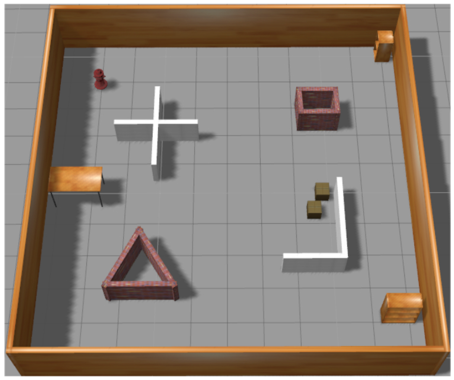
As the simulation environment for the training, we used a modified Gazebo world provided by [39], presented in Figure 3. Goal positions, as well as the robot’s starting position and pose at each episode were randomized. Since the depth images were received from only one camera that was located on the robot facing forwards, there was no reliable information about what was located behind the robot at all times. Consequently, the robot was not expected to move backward, and the minimum linear velocity was set as v m i n = 0 meters per second. During our training, the maximum linear velocity was set as v m a x = 0.5 meters per second and the maximum angular velocity was set to ω m a x = ± 1 radians per second. Each performed step in the simulation was recorded in a batch with a maximum size of 80,000. Each record consisted of { s t 1 , a t 1 , r ( s t , a t ) , c t , s t }, where c t represents the collision at time step t. Once the batch was full, old records were discarded and replaced with new ones. Network parameters were updated through learning from mini-batches of a size of 10 after each performed step. The loss was calculated as the mean squared error between the estimated Q-value and actual reward. The Adam Optimizer was used for loss minimization [45]. The list of network parameters used in training is presented in Table 1. We trained the network until the maximal Q-value converged, which took approximately 3000 episodes, taking 55 h.

5. Experiments

To validate the results of the training, experiments with the obtained network were conducted in two settings: a simulated environment in Gazebo and a real-life environment with inputs from a physical depth camera and a robot. In both setups, the same trained network was used to conduct the experiments. Quantitative and qualitative experiments were carried out where our method was compared with similar reactive obstacle avoidance approaches. For comparison purposes, we performed the same experiment with a map-less navigation method based on deep reinforcement learning proposed in [33], referred to as the ADDPG method. It employed an asynchronous DDPG network to learn navigation in a map-less environment based on single time step data of sparse laser readings and odometry. Training for this method was performed in the same environment as the CDDPG depth image-based method, depicted in Figure 3. An additional comparison was made with an Erle-rover laser obstacle avoidance package method for ROS simulations [46]. The Erle-rover method calculates the mean vector of laser readings and navigates in its direction, thus moving towards the empty space of the environment.

5.1. Experiments in the Simulated Environment

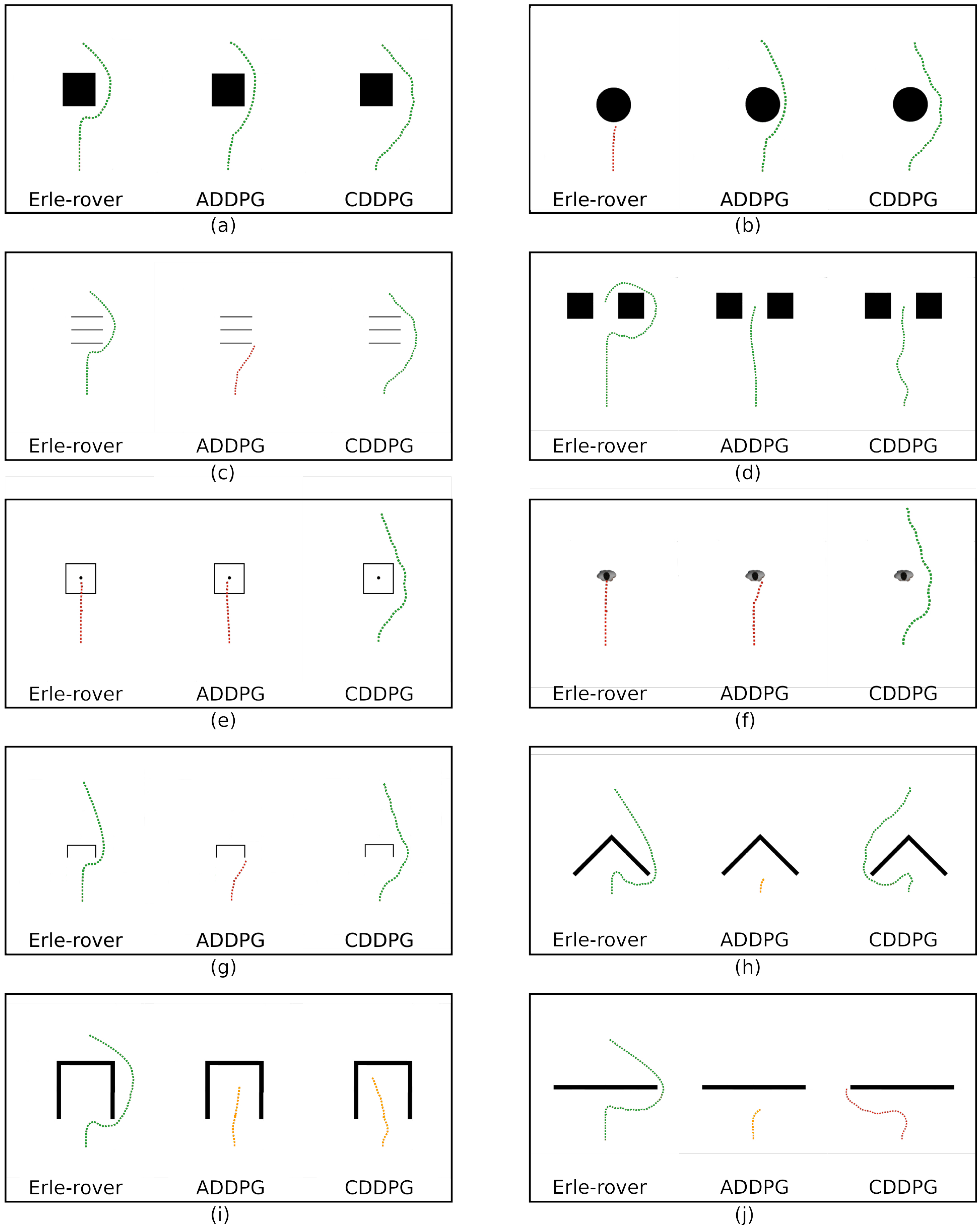
The main advantage of using input data from depth images is a more thorough scene representation. To show the benefit of a more complex representation of the environment through depth images over laser readings, avoidance around obstacles of varying complexity was explored. Naturally, a laser scan will only detect obstacles that are detectable on its plane, and a collision will occur with obstacles that cannot be perceived. However, also the geometrical composition of the obstacle can be a problem for laser-based obstacle avoidance, especially if sparse readings are used. Therefore, we performed comparison experiments of navigation around simulated objects of different compositions. This is portrayed in Figure 4. The robot had to navigate around the obstacle to a location behind it. In Figure 4d, the robot’s task was to navigate to a location between the two obstacles. From Figure 4, we can observe that sparse image readings had difficulty navigating around obstacles that did not have a solid shape. The sparse readings would register the distance to an obstacle at one time step, but after motion, would not register the obstacle at the next step. Here, a part of the obstacle would be located between the laser readings as is the case in Figure 4f, where the laser read the gap between the legs of a human and perceived it as a safe direction to move. A special case is depicted in Figure 4e, where a coffee table surface was located on a pole. The laser-based approaches could not perceive the narrow pole as an obstacle. On the contrary, the depth image collision avoidance could recognize the full shape of the obstacle and navigate around it. In the case of Figure 4h, the lack of local memory in ADDPG forced the robot to turn away and again towards an obstacle in consequent moves, thus freezing the robot and forcing it into a deadlock. However, such a situation could occur for our method as well if the robot finds itself in a situation where no improvement of the current location can be made over the span of its memory. This is portrayed in Figure 4i. Here, after navigating into the pocket, the robot would constantly turn for 10 steps in one direction and then 10 steps in the other in order to find a direction of safe movement. Since it was unable to find a safe direction, it was perpetually stuck in this motion. Due to the field of view angle restrictions of a single camera, our method may lack peripheral vision, which may lead to a collision in certain circumstances, as is depicted in Figure 4j. The robot navigated around an obstacle until it was not in view and began to turn. Since it was necessary to perform a large turn, the stack did not hold depth images of the obstacle and lost information about its location in relation to the robot.
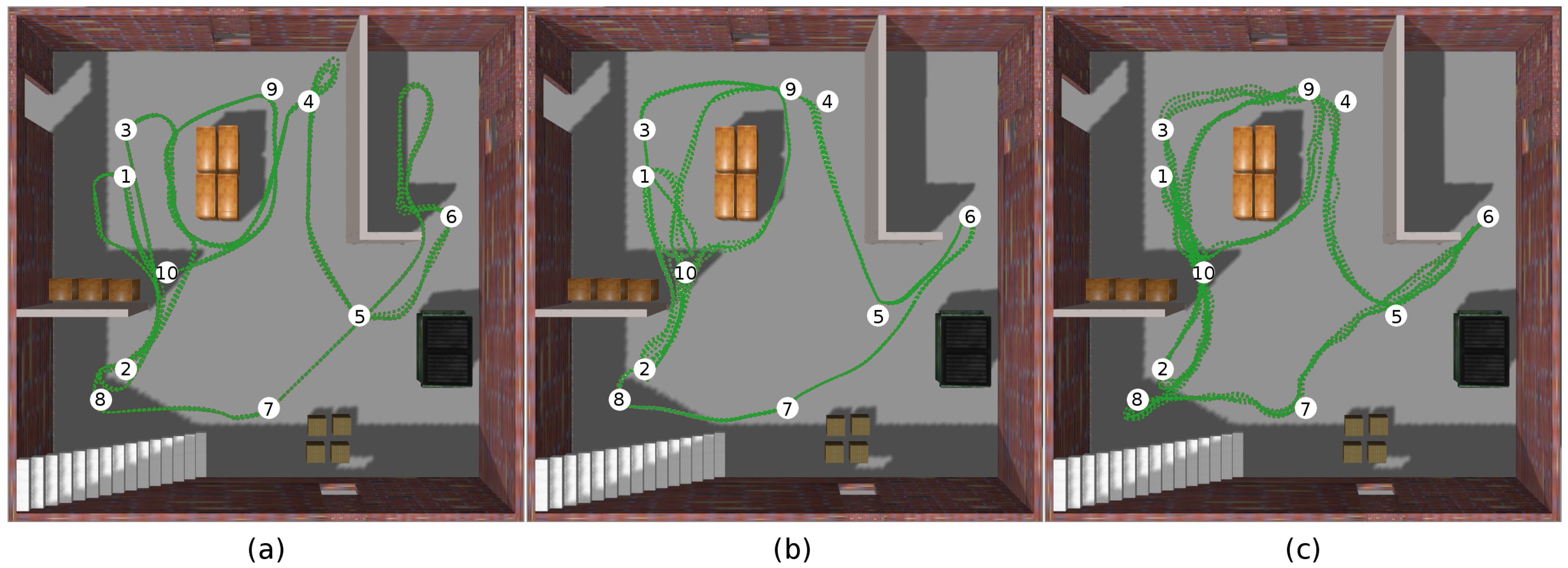
To compare the performance of the map-less navigation between multiple way-points in a simplified setting, we employed a simulated Gazebo environment. We designed a new Gazebo simulator environment for validation and performed the experiments using different obstacle models and layouts. The robot performed navigation over a course of 10 way-points for five laps in the environment while avoiding obstacles along the way. If the distance between the goal position and the robot’s estimated location was less than 30 centimeters, the goal was considered reached. As comparison metrics, we obtained the traveled distance in meters and navigation time in seconds. The performance of each method is displayed in Figure 5. The distance and time metrics over five laps are displayed in Table 2.
From the experiment, we could observe that using a more detailed sensory representation of the environment with a larger amount of data was comparable in terms of distance and time to that of ADDPG with sparse laser readings. The small increase of distance measured in our approach was due to more careful navigation around the obstacles, with an increased distance around them. The lack of peripheral vision forced the robot to keep an increased distance from the obstacles. Yet, the travel time was similar since the ADDPG method had difficulties navigating close to empty bookshelves, as is presented in Figure 4g. The shape of the bookshelves confused the navigation and forced the robot to slow down. By comparison, the rule-based approach of Erle-rover always led the robot along the safest path, disregarding a more optimal path towards the goal.

5.2. Experiments in a Real Environment

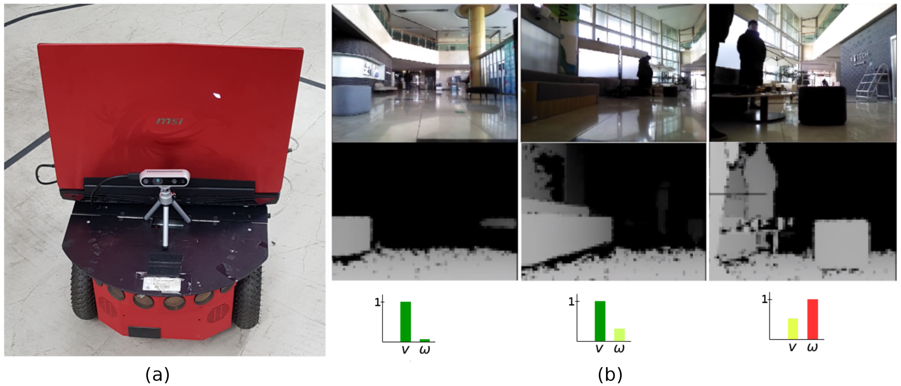
To prove the feasibility of the theoretical results obtained by the simulations, we performed experiments in a real environment and directly compared them to the results obtained by the ADDPG method. We used a Pioneer P3DX mobile robot platform on which we mounted an Intel Realsense D435 depth camera. For ADDPG implementation, we used a Velodyne Puck LiDAR scanner. A laptop with an NVIDIA GTX 980M graphics card, 32GB of RAM, and an Intel Core i7-5950HQ CPU was used to facilitate the networks. The robot setup is displayed in Figure 6a. The same as in the virtual simulation, the goal was considered to be reached at a distance of fewer than 30 centimeters. Just like during the training, the linear velocity was constrained to not exceed 0.5 m/s and the angular velocities not to exceed ±1 rad/s. An example of the proposed network output velocities in a real environment setting are presented in Figure 6b. If no obstacles were located in front of the robot, the network output the maximal linear and no angular velocity. If objects were in the way of the robot, the angular velocity was increased. When objects were close to the robot, the linear velocity was reduced and the angular velocity increased. In the presented case, the robot reduced it’s speed and performed a right turn.
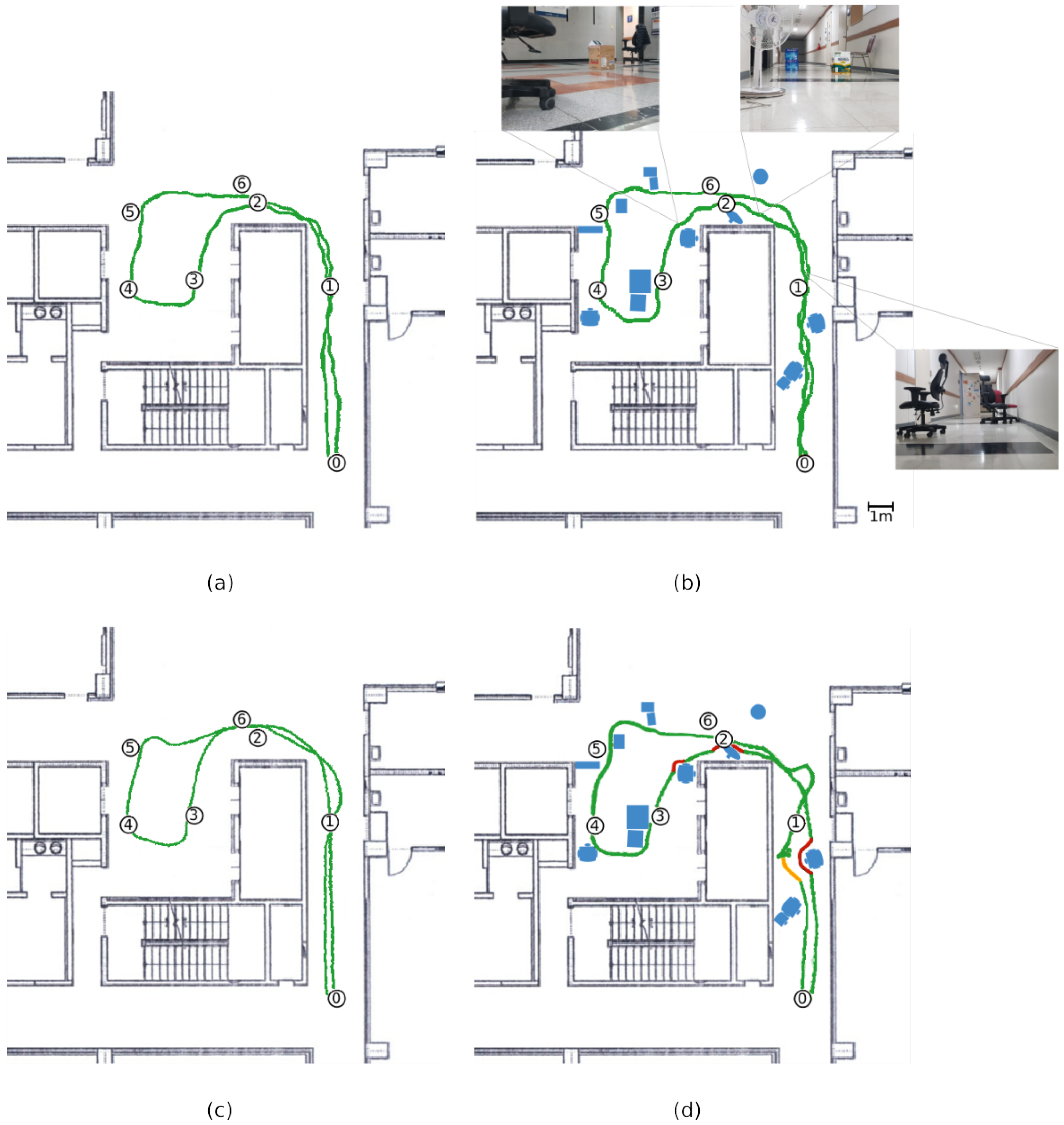
Experiments in a static environment were performed in an approximately 10 × 10 m 2 area. The robot navigated in the indoor environment arriving at the goal positions based on the sequence from 0 to 6 labeled in Figure 7. After reaching Point 6, the robot returned to the starting location. Experiments were performed in two settings. First, the CDDPG and ADDPG methods were used in an empty hallway, where the obstacles consisted of smooth walls, as visualized in Figure 7a,c, respectively. Afterward, interior objects such as chairs, fans, and boxes were added as obstacles for collision avoidance. Navigation in this environment is depicted in Figure 7b,d.
When using the CDDPG method, even though the environment was significantly different from the one during the training and the depth camera produced slightly different images from the ones in the simulation, the navigation system was able to recognize obstacles and navigate around them in both settings. The input from the depth camera could be noisy and differed significantly between sequential images. However, the effects of the noisy images were mitigated by adding random noise during the training stage. By comparison, the ADDPG method worked well in a hallway setting and could successfully navigate between the way-points. However, when additional complex obstacles were added in the environment, the ADDPG method failed to recognize or navigate around them. As depicted in Figure 7d, the robot was able to avoid such obstacles as boxes, but was unable to navigate around office chairs and a fan, where human intervention was required. Additionally, at a point where the robot was surrounded by multiple office chairs, it stalled, unable to find a clear way out of the situation. Human assistance was required to navigate the robot towards a clear path. The difference in performance was due to the laser reading passing through the mesh-like structure of the fan and registering only the support pole part of the chairs. On the contrary, our proposed approach was able to react to these obstacles. The navigation towards the goal did not differ significantly if objects were recognized. However, our proposed approach exhibited higher reliability in a varied environment.
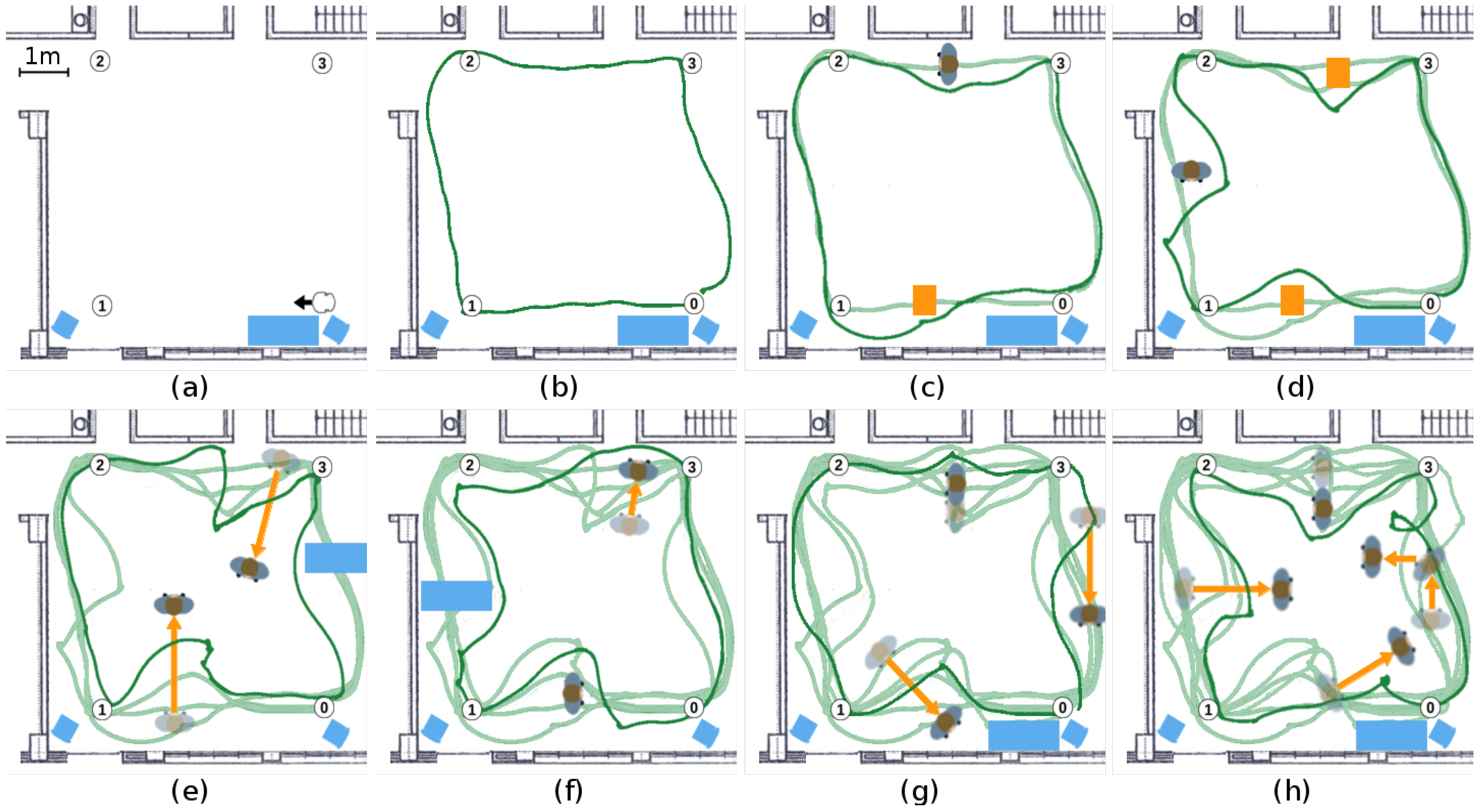
To show the capability of the proposed method working not only in static, but also dynamic environments, additional experiments were performed, as presented in Figure 8. These experiments were performed in an approximately 5 × 5 m 2 area, and four goal points were located at each of its corners. The experiment was performed by allowing the robot to navigate between the set goal points and introducing new obstacles, changing the location of previously existing obstacles and adding dynamic human obstacles. The initial layout with the location of the robot and its starting pose is presented in Figure 8a. In Figure 8b, the robot performed a circuit without obstacles between the goal points. New obstacles are introduced in Figure 8c,d. Dynamic obstacles in the form of a moving person are depicted in Figure 8e–h. The movement speed of the person was approximately matched to that of the robot. The person’s starting position was designated with an opaque and final position with a firm figure.
From these experiments, we could observe that upon introducing new or changing the location of previously seen obstacles, the robot still could perform avoidance and goal-oriented navigation. Changing the environment did not affect its performance. Moreover, our approach exhibited the capability of performing goal-oriented obstacle avoidance in the vicinity of moving obstacles. As was the case with a moving human, the robot was successful in recognizing it and finding a way to navigate around it. The robot reacted to dynamic human motion and produced motion based on it. Here, dynamic obstacle avoidance was possible without explicit motion data of the object. This showed that the CDDPG approach was capable of navigating in a dynamic environment. Additional experiments in static and dynamic environments can be viewed in the Supplementary Video https://youtu.be/nNWoabjKxIA.

6. Summary and Discussion

In this paper, a deep reinforcement learning-based algorithm was proposed for goal-oriented obstacle avoidance in continuous action space. Using depth images, a robot could safely navigate towards its goal while avoiding the obstacles. This was done by expanding the DDPG network to include depth-wise separable convolutional layers for processing the depth image data. The network could be trained in its entirety in a virtual simulator and directly transferred to be used in a real environment. Experiments were performed in both simulated and real environments to show the feasibility of the proposed network and compare it to existing approaches.
The depth image-based collision avoidance provided a more complete representation of obstacles than compared to laser-based methods. This allowed for safer navigation in environments filled with various structures. However, the choice of the number in the stack of sequential images n representing the state of the environment could be very important to how successfully the robot navigated. Since the network was not learning or mapping the features of the surroundings, the robot did not know the location of the obstacles, but rather, reacted to them when they came in view. Setting n to a value that was too low could result in a robot constantly turning towards the obstacle, once it was not in view anymore. The lack of peripheral view could be seen as a negative aspect of the proposed method as it could lead to a situation where an obstacle comes into view as the robot is turning, as shown in the experiments. This also means that the obstacle avoidance could fail if an object suddenly appeared in front of it at a close distance from the side. If an obstacle had previously not been observed, the robot would assume that the direction it was turning towards would be clear. Placing an obstacle on the side of the robot in such a case may lead to a collision. For this purpose, additional cameras on the sides of the robot or a laser sensor can be used in combination with the existing depth camera. A laser sensor should be located near the camera and scan the environment at a wider angle than the depth camera. This would allow collecting the data on the periphery. Since separate feature extraction should be performed, again, the mixed-input approach might need to be utilized to create sensor fusion within the network. The sensor fusion information would again be combined with the goal data to create a goal-oriented obstacle avoidance with sensor fusion. Such sensor fusion will be the focus of our ongoing research. Obtaining the depth images from a monocular camera instead of a depth camera, by applying a depth prediction network, is also considered. Here, pre-trained depth estimation from a monocular RGB camera network can be utilized to obtain depth images without the need for a depth camera. The output of the pre-trained network can be used as the input for obstacle avoidance, similarly to the approach presented in [39]. The effects of real depth camera noise can be mitigated by adding random noise to the simulated camera. Therefore, the network can be implemented in real-life scenarios as-is from training only in simulation. However, further training of the network in a real environment could improve the smoothness of the robot motion in real-life settings. This will be explored in the future.

Author Contributions

The authors confirm the contribution to the paper as follows: concept idea, design, software, and validation: R.C.; concept idea, design, and supervision: J.H.L. and I.H.S.; writing, original draft preparation: R.C.; writing, review and editing: J.H.L. and I.H.S. All authors read and agreed to the published version of the manuscript.

Funding

This work was supported by the Technology Innovation Program (Industrial Strategic Technology Development, 10080638) funded by the Ministry of Trade, Industry & Energy (MOTIE), Republic of Korea.

Conflicts of Interest

The authors declare no conflict of interest.

Abbreviations

The following abbreviations are used in this manuscript:
RRT*Rapidly-exploring Random Tree Star
SLAMSimultaneous Localization and Mapping
D3QNDeep Double Q Network
DDPGDeep Deterministic Policy Gradient
ADDPGAsynchronous Deep Deterministic Policy Gradient
CDDPGConvolutional Deep Deterministic Policy Gradient
ReLURectified Linear Unit
ROSRobot Operating System

References

  1. Sifre, L.; Mallat, S. Rigid-motion scattering for texture classification. arXiv 2014, arXiv:1403.1687. [Google Scholar]
  2. Howard, A.G.; Zhu, M.; Chen, B.; Kalenichenko, D.; Wang, W.; Weyand, T.; Andreetto, M.; Adam, H. Mobilenets: Efficient convolutional neural networks for mobile vision applications. arXiv 2017, arXiv:1704.04861. [Google Scholar]
  3. Sandler, M.; Howard, A.; Zhu, M.; Zhmoginov, A.; Chen, L.C. Mobilenetv2: Inverted residuals and linear bottlenecks. In Proceedings of the IEEE Conference on Computer Vision and Pattern Recognition, Salt Lake City, UT, USA, 18–22 June 2018; pp. 4510–4520. [Google Scholar]
  4. Sariff, N.; Buniyamin, N. An overview of autonomous mobile robot path planning algorithms. In Proceedings of the 2006 4th Student Conference on Research and Development, Selangor, Malaysia, 27–28 June 2006; pp. 183–188. [Google Scholar]
  5. Radmanesh, M.; Kumar, M.; Guentert, P.H.; Sarim, M. Overview of path-planning and obstacle avoidance algorithms for UAVs: A comparative study. Unmanned Syst. 2018, 6, 95–118. [Google Scholar] [CrossRef]
  6. Noreen, I.; Khan, A.; Habib, Z. A comparison of RRT, RRT* and RRT*-smart path planning algorithms. Int. J. Comput. Sci. Netw. Secur. (IJCSNS) 2016, 16, 20. [Google Scholar]
  7. Kim, Y.N.; Ko, D.W.; Suh, I.H. Confidence random tree-based algorithm for mobile robot path planning considering the path length and safety. Int. J. Adv. Rob. Syst. 2019, 16, 1729881419838179. [Google Scholar] [CrossRef]
  8. Cimurs, R.; Suh, I.H. Time-optimized 3D Path Smoothing with Kinematic Constraints. Int. J. Control Autom. Syst. 2020. [Google Scholar] [CrossRef]
  9. Ribeiro, J.; Silva, M.; Santos, M.; Vidal, V.; Honório, L.; Silva, L.; Rezende, H.; Neto, A.S.; Mercorelli, P.; Pancoti, A. Ant Colony Optimization Algorithm and Artificial Immune System Applied to a Robot Route. In Proceedings of the 2019 20th International Carpathian Control Conference (ICCC), Krakow-Wieliczka, Poland, 26–29 May 2019; pp. 1–6. [Google Scholar]
  10. Lamini, C.; Benhlima, S.; Elbekri, A. Genetic algorithm based approach for autonomous mobile robot path planning. Procedia Comput. Sci. 2018, 127, 180–189. [Google Scholar] [CrossRef]
  11. Cimurs, R.; Hwang, J.; Suh, I.H. Bezier curve-based smoothing for path planner with curvature constraint. In Proceedings of the 2017 First IEEE International Conference on Robotic Computing (IRC), Taichung, Taiwan, 10–12 April 2017; pp. 241–248. [Google Scholar]
  12. Ferguson, D.; Stentz, A. Field D*: An interpolation-based path planner and replanner. In Robotics Research; Springer: Berlin/Heidelberg, Germany, 2007; pp. 239–253. [Google Scholar]
  13. Ferguson, D.; Stentz, A. The Field D* Algorithm for Improved Path Planning and Replanning in Uniform and Non-Uniform Cost Environments; Tech. Rep. CMU-RI-TR-05-19; Robotics Institute, Carnegie Mellon University: Pittsburgh, PA, USA, 2005. [Google Scholar]
  14. Dolgov, D.; Thrun, S.; Montemerlo, M.; Diebel, J. Path planning for autonomous vehicles in unknown semi-structured environments. Int. J. Robot. Res. 2010, 29, 485–501. [Google Scholar] [CrossRef]
  15. Taketomi, T.; Uchiyama, H.; Ikeda, S. Visual SLAM algorithms: A survey from 2010 to 2016. IPSJ Trans. Comput. Vis. Appl. 2017, 9, 16. [Google Scholar] [CrossRef]
  16. Fuentes-Pacheco, J.; Ruiz-Ascencio, J.; Rendón-Mancha, J.M. Visual simultaneous localization and mapping: A survey. Artif. Intell. Rev. 2015, 43, 55–81. [Google Scholar] [CrossRef]
  17. Ko, D.W.; Kim, Y.N.; Lee, J.H.; Suh, I.H. A scene-based dependable indoor navigation system. In Proceedings of the 2016 IEEE/RSJ International Conference on Intelligent Robots and Systems (IROS), Daejeon, Korea, 9–14 October 2016; pp. 1530–1537. [Google Scholar]
  18. Lin, J.; Wang, W.J.; Huang, S.K.; Chen, H.C. Learning based semantic segmentation for robot navigation in outdoor environment. In Proceedings of the 2017 Joint 17th World Congress of International Fuzzy Systems Association and 9th International Conference on Soft Computing and Intelligent Systems (IFSA-SCIS), Otsu, Japan, 27–30 June 2017; pp. 1–5. [Google Scholar]
  19. Zhang, Y.; Chen, H.; He, Y.; Ye, M.; Cai, X.; Zhang, D. Road segmentation for all-day outdoor robot navigation. Neurocomputing 2018, 314, 316–325. [Google Scholar] [CrossRef]
  20. Niijima, S.; Sasaki, Y.; Mizoguchi, H. Real-time autonomous navigation of an electric wheelchair in large-scale urban area with 3D map. Adv. Robot. 2019, 33, 1006–1018. [Google Scholar] [CrossRef]
  21. Pham, H.; Smolka, S.A.; Stoller, S.D.; Phan, D.; Yang, J. A survey on unmanned aerial vehicle collision avoidance systems. arXiv 2015, arXiv:1508.07723. [Google Scholar]
  22. Hoy, M.; Matveev, A.S.; Savkin, A.V. Algorithms for collision-free navigation of mobile robots in complex cluttered environments: A survey. Robotica 2015, 33, 463–497. [Google Scholar] [CrossRef] [Green Version]
  23. Garcia-Cruz, X.; Sergiyenko, O.Y.; Tyrsa, V.; Rivas-Lopez, M.; Hernandez-Balbuena, D.; Rodriguez-Quiñonez, J.; Basaca-Preciado, L.; Mercorelli, P. Optimization of 3D laser scanning speed by use of combined variable step. Opt. Lasers Eng. 2014, 54, 141–151. [Google Scholar] [CrossRef]
  24. Ivanov, M.; Sergiyenko, O.; Tyrsa, V.; Mercorelli, P.; Kartashov, V.; Hernandez, W.; Sheiko, S.; Kolendovska, M. Individual scans fusion in virtual knowledge base for navigation of mobile robotic group with 3D TVS. In Proceedings of the IECON 2018-44th Annual Conference of the IEEE Industrial Electronics Society, Washington, DC, USA, 21–23 October 2018; pp. 3187–3192. [Google Scholar]
  25. Mnih, V.; Kavukcuoglu, K.; Silver, D.; Rusu, A.A.; Veness, J.; Bellemare, M.G.; Graves, A.; Riedmiller, M.; Fidjeland, A.K.; Ostrovski, G.; et al. Human-level control through deep reinforcement learning. Nature 2015, 518, 529. [Google Scholar] [CrossRef]
  26. Dann, M.; Zambetta, F.; Thangarajah, J. Integrating skills and simulation to solve complex navigation tasks in Infinite Mario. IEEE Trans. Games 2018, 10, 101–106. [Google Scholar] [CrossRef]
  27. Tampuu, A.; Matiisen, T.; Kodelja, D.; Kuzovkin, I.; Korjus, K.; Aru, J.; Aru, J.; Vicente, R. Multiagent cooperation and competition with deep reinforcement learning. PLoS ONE 2017, 12, e0172395. [Google Scholar] [CrossRef]
  28. Ding, X.; Zhang, Y.; Liu, T.; Duan, J. Deep learning for event-driven stock prediction. In Proceedings of the Twenty-Fourth International Joint Conference on Artificial Intelligence, Buenos Aires, Argentina, 25–31 July 2015. [Google Scholar]
  29. Akita, R.; Yoshihara, A.; Matsubara, T.; Uehara, K. Deep learning for stock prediction using numerical and textual information. In Proceedings of the 2016 IEEE/ACIS 15th International Conference on Computer and Information Science (ICIS), Okayama, Japan, 26–29 June 2016; pp. 1–6. [Google Scholar]
  30. Chong, E.; Han, C.; Park, F.C. Deep learning networks for stock market analysis and prediction: Methodology, data representations, and case studies. Expert Syst. Appl. 2017, 83, 187–205. [Google Scholar] [CrossRef] [Green Version]
  31. Sünderhauf, N.; Brock, O.; Scheirer, W.; Hadsell, R.; Fox, D.; Leitner, J.; Upcroft, B.; Abbeel, P.; Burgard, W.; Milford, M.; et al. The limits and potentials of deep learning for robotics. Int. J. Robot. Res. 2018, 37, 405–420. [Google Scholar]
  32. Tai, L.; Li, S.; Liu, M. A deep-network solution towards model-less obstacle avoidance. In Proceedings of the 2016 IEEE/RSJ International Conference on Intelligent Robots and Systems (IROS), Daejeon, South Korea, 9–14 October 2016; pp. 2759–2764. [Google Scholar]
  33. Tai, L.; Paolo, G.; Liu, M. Virtual-to-real deep reinforcement learning: Continuous control of mobile robots for mapless navigation. In Proceedings of the 2017 IEEE/RSJ International Conference on Intelligent Robots and Systems (IROS), Vancouver, BC, Canada, 24–28 September 2017; pp. 31–36. [Google Scholar]
  34. Zhu, Y.; Mottaghi, R.; Kolve, E.; Lim, J.J.; Gupta, A.; Fei-Fei, L.; Farhadi, A. Target-driven visual navigation in indoor scenes using deep reinforcement learning. In Proceedings of the 2017 IEEE international conference on robotics and automation (ICRA), Singapore, 29 May–3 June 2017; pp. 3357–3364. [Google Scholar]
  35. Richter, C.; Roy, N. Safe visual navigation via deep learning and novelty detection. In Proceedings of the Robotics: Science and Systems XIII, Cambridge, MA, USA, 12–16 July 2017. [Google Scholar]
  36. Zhang, J.; Springenberg, J.T.; Boedecker, J.; Burgard, W. Deep reinforcement learning with successor features for navigation across similar environments. In Proceedings of the 2017 IEEE/RSJ International Conference on Intelligent Robots and Systems (IROS), Vancouver, BC, Canada, 24–28 September 2017; pp. 2371–2378. [Google Scholar]
  37. Giusti, A.; Guzzi, J.; Cireşan, D.C.; He, F.L.; Rodríguez, J.P.; Fontana, F.; Faessler, M.; Forster, C.; Schmidhuber, J.; Di Caro, G.; et al. A machine learning approach to visual perception of forest trails for mobile robots. IEEE Robot. Autom. Lett. 2016, 1, 661–667. [Google Scholar] [CrossRef] [Green Version]
  38. Kahn, G.; Villaflor, A.; Pong, V.; Abbeel, P.; Levine, S. Uncertainty-aware reinforcement learning for collision avoidance. arXiv 2017, arXiv:1702.01182. [Google Scholar]
  39. Xie, L.; Wang, S.; Markham, A.; Trigoni, N. Towards monocular vision based obstacle avoidance through deep reinforcement learning. arXiv 2017, arXiv:1706.09829. [Google Scholar]
  40. Wang, Y.; He, H.; Sun, C. Learning to navigate through complex dynamic environment with modular deep reinforcement learning. IEEE Trans. Games 2018, 10, 400–412. [Google Scholar] [CrossRef]
  41. Lillicrap, T.P.; Hunt, J.J.; Pritzel, A.; Heess, N.; Erez, T.; Tassa, Y.; Silver, D.; Wierstra, D. Continuous control with deep reinforcement learning. arXiv 2015, arXiv:1509.02971. [Google Scholar]
  42. Rusu, A.A.; Vecerik, M.; Rothörl, T.; Heess, N.; Pascanu, R.; Hadsell, R. Sim-to-real robot learning from pixels with progressive nets. arXiv 2016, arXiv:1610.04286. [Google Scholar]
  43. James, S.; Johns, E. 3d simulation for robot arm control with deep q-learning. arXiv 2016, arXiv:1609.03759. [Google Scholar]
  44. Silver, D.; Lever, G.; Heess, N.; Degris, T.; Wierstra, D.; Riedmiller, M. Deterministic policy gradient algorithms. In Proceedings of the International Conference on Machine Learning (ICML), Beijing, China, 21–26 June 2014; pp. 387–395. [Google Scholar]
  45. Kingma, D.P.; Ba, J. Adam: A method for stochastic optimization. arXiv 2014, arXiv:1412.6980. [Google Scholar]
  46. ROS. Erle-Rover. 2016. Available online: http://wiki.ros.org/Robots/Erle-Rover (accessed on 4 July 2019).
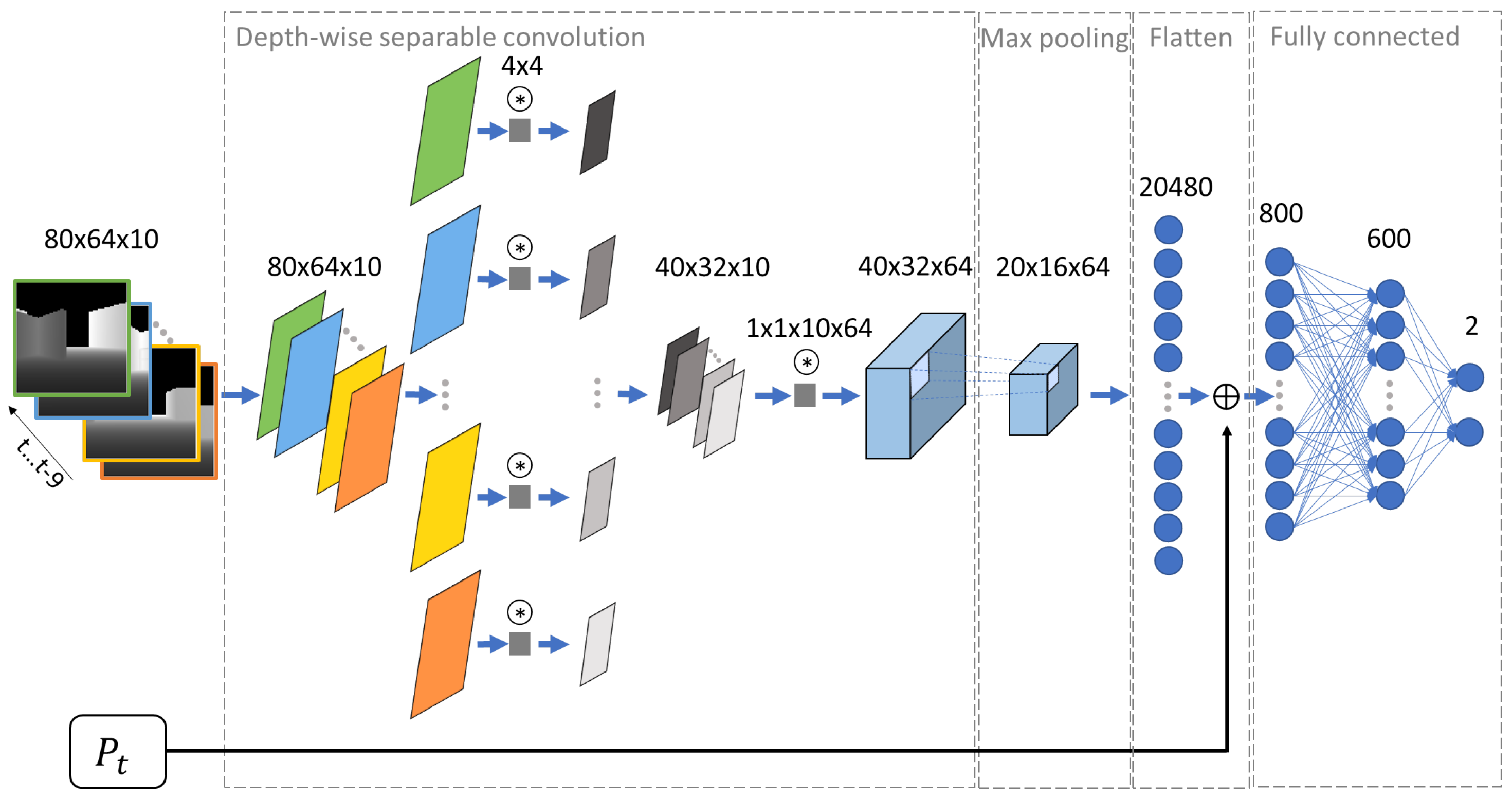
Figure 1. Architecture of the proposed actor network. Depth-wise separable convolution is performed on a stack of depth images. Max pooling is performed on the output. Positional information is concatenated with the depth information, followed by two fully connected layers and an output layer. ⊛ and ⊕ denote convolution and concatenation, respectively.
Electronics 09 00411 g001
Figure 2. Full architecture of the proposed network including the actor and critic parts. Both parts of the network use the same depth and position information as state inputs. The calculated actions from the actor are sent to the critic to update the network parameters. ⊛ and ⊕ denote convolution and concatenation, respectively.
Electronics 09 00411 g002
Figure 3. Environment in the Gazebo simulator for training.
Electronics 09 00411 g003
Figure 4. Simulation results with the shapes of different geometrical compositions. The green path designates successful motion. The red path indicates a motion resulting in a collision. The orange path designates a situation where the robot encounters a deadlock. (a) Cube, (b) sphere, (c) 3 thin walls, (d) goal point between two cubes, (e) a coffee table with a surface on a pole, (f) person, (g) empty bookshelf, (h) concave corner, (i) room, (j) long wall.
Electronics 09 00411 g004
Figure 5. Validation odometry information in a simulated environment. Numbers depict the sequence in which the robot needs to navigate to designated points. The green path visualizes the trajectory of each respective method. (a) Experimental results of the Erle-rover laser-based method. (b) Experimental results of the ADDPG sparse laser-based method. (c) Experimental results of the CDDPG depth image-based method.
Electronics 09 00411 g005
Figure 6. (a) Robot setup for experiments in a real environment. (b) Example of network outputs in a real environment. An RGB image is shown for visualization purposes, and the proposed network uses only provided depth images. v represents the linear and ω angular velocities, respectively. One represents the maximal possible value of the respective velocity.
Electronics 09 00411 g006
Figure 7. Results in the real environment. The green path depicts the robot’s movements from odometry data. Red parts of the path show the human intervention after a crash. The orange part of the path shows the human intervention after the robot encountered a deadlock. Blue shapes depict the location and shape of the obstacles. Numbers from 0 to 6 describe the locations and sequence of the target goals. Images show the robot’s view of the environment at the location. (a) CDDPG performance in an environment without added obstacles; (b) CDDPG performance in an environment with added obstacles; (c) ADDPG performance in an environment without added obstacles; (d) ADDPG performance in an environment with added obstacles.
Electronics 09 00411 g007
Figure 8. Results in the dynamic environment. The green path depicts the robot’s movements from odometry data. Blue shapes depict obstacles already in the scene, and orange shapes depict newly introduced obstacles. A human obstacle was introduced in the scene, and if it was in motion, its opaque shape designated the starting position of the motion. The motion direction is visualized by an orange arrow. Numbers from 0 to 3 describe the locations and sequence of the target goals. (a) Layout of the experiment environment. (b) Experiment without obstacles. (c,d) Experiments with new static obstacles. (e,f) Experiments with relocated static and dynamic human obstacles. (g,h) Experiments with dynamic human obstacles.
Electronics 09 00411 g008
Table 1. CDDPG network learning parameters during training.
ParameterValue
Actor Network Learning Rate0.0001
Critic Network Learning Rate0.001
Critic Network Discount Factor0.99
Soft Target Update Parameter0.001
Buffer Size80,000
Mini-Batch Size10
Random Seed Value1234
Table 2. Experimental results for each method over individual laps and average score. Distance is expressed in meters and time in seconds.
Distance (m) Time (s)
Erle-roverADDPGCDDPGErle-roverADDPGCDDPG
Lap 162.0146.2449.78168128123
Lap 263.2546.7449.97173126129
Lap 363.4146.4749.64171127125
Lap 463.6946.6649.87172125123
Lap 563.8446.6150.05172122126
Average63.2446.5449.86171.2125.6125.2