Abstract
Radio frequency interference has become a rising problem to the signal of the Global Navigation Satellite System (GNSS). An effective way to achieve anti-jamming is by using an antenna array in GNSS signal processing. However, antenna array processing will cause a decline in the accuracy of pseudo-range measurements because of the channel mismatch and some other non-ideal factors. To solve this problem, space–time or space–frequency adaptive array processing is widely used for interference cancellation while constraining the delay of each antenna at the same time. In this paper, an anti-jamming algorithm with a time-delay constraint is proposed, where one antenna is chosen as the reference and data from other antennas is corrected based on the signal received from it. The deduction and simulation results show that the proposed algorithm can effectively improve the accuracy of pseudo-range measurements without degradation of anti-jamming performance.
1. Introduction
The Global Navigation Satellite System (GNSS) has been widely used in many fields like transportation and aviation, which has greatly changed our daily lives [1,2]. There are many indicators showing the performance of GNSS receivers, such as usability, accuracy, integrity, and continuity, of which accuracy is one of the most important indicators for high precision applications [3,4,5].
However, because of the low broadcasting power and long transmitting distance, the GNSS signal is easily jammed by unintentional or intentional Radio Frequency Interference (RFI) [6,7], which has become a rising problem to high precision GNSS applications. To mitigate the influence of RFI, antenna array processing is widely used in military and some other high-end applications, because it can suppress not only narrow-band but also broadband interference [8,9]. Unfortunately, although the antenna array processing can effectively suppress RFI, it will introduce Pseudo-Range (PR) bias and affect the positioning accuracy of GNSS receivers. For example, it is shown in [10] that the PR measurement deviation introduced by the array processing is in the order of 10 ns, which prevents the array processing being used in some high accuracy-requiring scenarios where the PR measurement deviation is usually suppressed to less than 1 ns, such as the guided missiles, measurement receivers, aircraft landing systems, and so on [11,12,13]. Therefore, it is important to study the influence of antenna array anti-jamming processing on PR measurements and its improvement [14].
Much research has been done to study the effect of RFI and anti-jamming array processing on PR measurement. It can be proved that when applying the narrow-band GNSS array signal model, where the time delays of different signal frequencies are neglected, the Space Array Processing (SAP) does not cause bias in PR measurement because the received signals of each antenna only differ in carrier phase, and the weights of SAP will not affect the baseband signals of each antenna, so that high-precision of PR measurements can be achieved [15,16]. However, it has been analyzed in [17], that when the transmission channel is not ideal, the SAP is no longer effective in suppressing RFI because the non-ideality will result in a loss of array freedom in the time domain. In this case, the Space–Time Array Processing (STAP) should be chosen instead of the SAP to enhance the performance of RFI suppression. Although many studies have shown the superiority of the anti-jamming performance of STAP, the space–time filter will cause a deviation of PR measurements [18]. Therefore, the performance of anti-jamming and high precision seems to be incompatible when using the traditional SAP and STAP.
In this paper, an anti-jamming algorithm with time-delay constraint is proposed to achieve high precision PR measurements in array anti-jamming processing. In the proposed algorithm, one antenna is chosen as the reference, and data of other antennas is corrected based on the receiving signal of it, which can constrain the delay of each channel. The rest of this paper is arranged as follows: Firstly, Section 2 introduces the array model used in this paper. Secondly, in Section 3, the effect of STAP is analyzed, including the effect on Auto Correlation Function (ACF) distortion and accuracy of PR measurements. Then in Section 4, the ranging deviation suppression algorithm is proposed. After that, the simulation results are shown and analyzed in Section 5. Finally, the conclusion is drawn in Section 6.
2. Array Model
According to [19], the accuracy of pseudo-code ranging is related to the array style, and the center plane array structure is often used in high-precision applications, because in the ideal case, the phase center of this style is the geometric center, and the performance of it can be compared with that of the single antenna at the center. Therefore, the four-antenna central plane array is considered, and the central antenna is chosen as the reference in this paper, as shown in Figure 1.
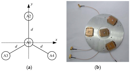
Figure 1.
Four elements with central plane array. (a) Model; (b) Physical.
In this case, the array element coordinates of the four antennas are
In general, the distance between two antennas is half a wavelength and can be expressed as:
where is the wavelength of the GNSS signal, is the corresponding radio frequency, and is the propagation speed of the radio wave.
The propagation delay of the signal between one antenna and the reference can be expressed as
where stands for the coordinate of that antenna, are the azimuth and elevation angle of received signal, respectively.
The steering vector can be denoted as
Hence, the array data can be expressed as [20]
where and are the numbers of interference and signal, respectively. is the interference signal, is the GNSS signal, and is the noise vector.
The correlation matrix of received data can be expressed as [21]
The Power Inversion (PI) is a typical blind anti-jamming criterion which does not need any prior information except a correlation matrix [22]. It nulls in the direction of strong interference by adapting the weights of antennas and is particularly suitable in the case of a weak desired signal with strong interference, such as GNSS anti-jamming processing. Therefore, the PI criterion is chosen in this paper, and the constraints of PI can be expressed as
where is the constraint vector that prevents the weights converging on zero, and it can be expressed as
An enhancement of array processing is to use STAP, which adapts time domain weights to increase the degree of array freedom without adding antennas. Figure 2 shows the STAP with elements and taps. Typically, in SAP the taps is 1.
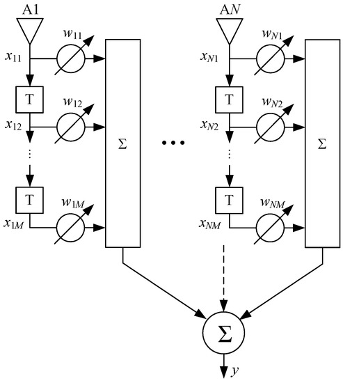
Figure 2.
Space–Time Array Processing (STAP) structure.
For the STAP structure, the sampled data in the space–time domain is composed of the received data in different sampling times, and it can be written as
where is the vector of received data in corresponding to Equation (8) in SAP, is the delay time of each tap, which is also the sampling interval.
The weights can be expressed as
The calculation method of Equation (13) can also be referred to Equations (9) and (10).
Therefore, the array output can be denoted as the weighting summation of each sampled data tap as
3. Effect of STAP on PR Accuracy
In this section, two aspects of the effect of STAP in anti-jamming are analyzed. On the one hand, a new and uncertain delay is introduced by STAP because of the delay of the space–time adaptive filter. On the other hand, the ACF peak will be unintentionally distorted as well.
3.1. Analysis of Delay Uncertainty
According to the analysis of [19] and [20], the purpose of the space–time adaptive filter is to mitigate the inconsistency of signal transmission channels. However, the characteristics of each channel may be different, and the group delay of the space–time adaptive filter is also related to many factors such as time-domain taps, interference power, interference type, interference direction, channel characteristics, and so on [23]. Therefore, the delay of space–time adaptive filter is actually uncertain.
Considering a two antenna array as an example, some typical testing scenarios are shown in Table 1.

Table 1.
Scenario settings.
The group delays in these scenarios are shown in Figure 3, which verifies the uncertainty of the space–time adaptive filter group delay.
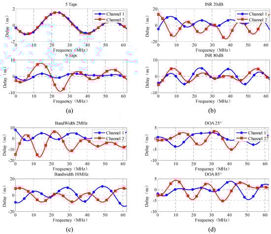
Figure 3.
Group delay of equivalent filter. (a) Scenario 1#; (b) Scenario 2#; (c) Scenario 3#; (d) Scenario 4#.
3.2. Analysis of Correlation Peak Distortion
In Equation (14), and are the weight and the input data. Since may not be linear phase, the weighting process can be treated as introducing multipath signal; thus the ACF will be distorted. Similar to the group delay of filter, is also related to many factors such as time-domain taps, interference power, interference type, interference direction, channel characteristics, etc., and all of these factors are uncontrollable. As directly determines the ACF distortion, the effect of space–time filter on ACF distortion is also uncertain.
The simulation was carried out based on the scenarios in Table 1. Applying the analysis method of [24], the combined signal of the GNSS signal, interference, and noise was used to generate the weight of STAP, while the ACFs were plotted only by weighting the GNSS signal, which is shown in Figure 4.
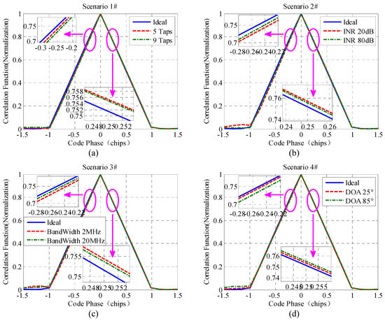
Figure 4.
Impact on correction function. (a) Scenario 1#; (b) Scenario 2#; (c) Scenario 3#; (d) Scenario 4#.
Figure 4 verifies the uncertainty of ACF distortion caused by the space–time adaptive filter. According to Figure 4, the effect of the space–time adaptive filter on the signal SCB (S Curve Bias) curve is shown in Figure 5.
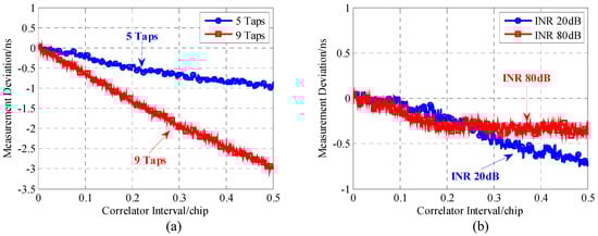
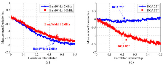
Figure 5.
Impact on S Curve Bias (SCB) curve. (a) Scenario 1#; (b) Scenario 2#; (c) Scenario 3#; (d) Scenario 4#.
It can be noted from Figure 5 that there are significant differences in PR measurement deviations in different scenarios. Particularly when the correlation interval is 0.5 chips, the PR measurement deviation reaches 3 ns in the case of Scenario 1#.
Therefore, the space–time adaptive filter not only causes the position of ACF peak to shift, but also causes the shape of ACF peak to be distorted, which means the conventional space–time adaptive filter can lead to an uncontrollable deviation of pseudo-code ranging.
4. Anti-jamming algorithm with Constrained Delay
The SAP and STAP have the following contradictions between the performance of interference suppression and PR measurement accuracy:
(1) The SAP can ensure the accuracy of PR measurement, but the anti-jamming performance will greatly degrade.
(2) The STAP can improve the anti-jamming performance, but the PR measurement will have uncertain deviation.
According to [19], the purpose of STAP is to mitigate the difference in channel transmission characteristics and improve the data consistency of each antenna.
According to the analysis in [23], the space–time processing method is used for anti-jamming, or the space anti-jamming is used after channel correction. The model is shown in Figure 6.
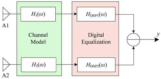
Figure 6.
Relationship between channel and digital filter.
In the model of Figure 6, and determine the PR measurement of each channel, and the following equation is satisfied when the interference is effectively suppressed:
where and are the models of antenna channels which are determined by the inherent properties of hardware, whose digital characteristics are uncontrollable but basically stable. and are determined by the digital space–time filters applying the traditional PI criterion. According to the analysis in Section 3.1, the delay of the digital filter is uncontrollable and is related to many factors.
To solve the problem of uncontrollable digital filter delay, an anti-jamming processing structure with one reference antenna is proposed, as seen in Figure 7.
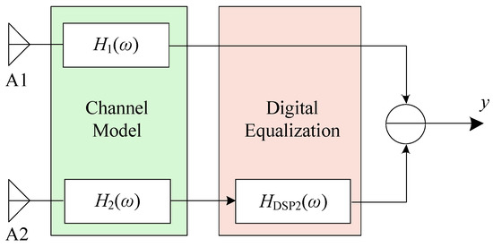
Figure 7.
Anti-jamming processing framework.
When applying the structure of Figure 7, the constraint that interference is effectively suppressed can be adapted as
where and are still determined by the properties of antennas, but is adapted to make sure Equation (16) is satisfied. Therefore, the total delay of the channel and digital filter is determined by , and the anti-jamming filter does not cause additional delay.
For the structure of Figure 6 with one reference antenna, this paper proposes a space only anti-jamming algorithm based on channel relative correction. In [23], the channel relative correction method for constrained reference array antennas has been proposed, and it has been proved that after relative correction of channel, the interference suppression can be realized by SAP rather than STAP. In the proposed algorithm, the received signal from the reference antenna does not pass the digital filter, and therefore the process of weighting will not cause additional distortion. The structure of the proposed algorithm is shown in Figure 8.
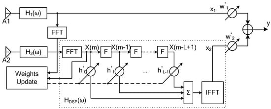
Figure 8.
Space only anti-jamming processing framework.
In Figure 8, and are channel models of antenna determined by hardware, while is the channel model of the correction filter. When the channel is effectively corrected, satisfies the constraint equation (Equation (14)). The weight is generated in the frequency domain, as well as the channel correction.
Compared with the algorithm in [23], which applies STAP after relative correction, the proposed algorithm in this section uses the simpler SAP and can effectively suppress the interference in [23]. However, the proposed algorithm enhances the computational complexity compared to the traditional SAP due to the relative correction between channels. Besides, to achieve the optimal interference suppression, more FFT points are needed, which requires more computing resources. As the channel characteristics cannot be quantitatively analyzed, the extra computing complexity cannot be precisely calculated either.
5. Simulation Experiment
5.1. Interference Suppression Performance
The testing scenarios in Table 1 were used for simulation, and the interference suppression comparison of traditional algorithm and proposed algorithm is shown in Table 2, where Difference stands for the difference of anti-jamming performance. It can be seen from Table 2 that the influence of delay constraint on the anti-jamming performance was small compared with that of the traditional algorithm, and the difference between two algorithms was less than 1 dB in the testing scenarios.
Table 2.
Interference suppression ratio.
As seen in Table 2, the anti-jamming performance differed between the traditional and the proposed algorithm.
5.2. Anti-jamming Processing Delay
In Figure 9, different channel delays of equivalent filter groups are presented, which were based on the scenarios of Table 1 while applying the proposed algorithm. The delays were significantly mitigated to less than 0.2 ns by the proposed algorithm, compared with a maximum of 30 ns in Figure 2, which applied the traditional STAP.
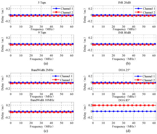
Figure 9.
Equivalent filter delay of each element under delay constraints. (a) Scenario 1#; (b) Scenario 2#; (c) Scenario 3#; (d) Scenario 4#.
5.3. Correlation Function Distortion
As shown in Figure 3, it was difficult to compare the correlation-function distortion by the ACF peak. On the other hand, the SCB curve clearly showed the correlation-function distortion and the deviation of range. Therefore, the SCB curves based on scenarios of Table 1 while applying the proposed algorithm are presented in Figure 10.
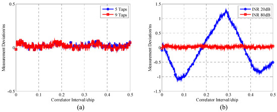
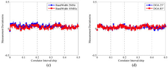
Figure 10.
SCB curve under time delay constraints. (a) Scenario 1#; (b) Scenario 2#; (c) Scenario 3#; (d) Scenario 4#.
The PR measurement deviation was effectively suppressed by the proposed algorithm, whose maximum decreased to 1.3 ns compared to 4 ns in Figure 5. It can be noted that except for Scenario 2#, in which INR was 20 dB, the deviations in other scenarios were less than 0.5 ns. The reason for the 1.3 ns deviation in Scenarios 2# is that when the INR was 20 dB, the correlation of interference between different antennas was weak, and the array weights had volatility waving.
5.4. Software Receiver Emulation
Three different anti-jamming algorithms were simulated by the Software Defined Receiver (SDR) to compare the auto-adaptive performance, including the SAP, the STAP and the proposed algorithm. Besides, the directly-passing (no interference) simulation was also carried out to set up a reference. In a 1000 ms simulation, the variation of interference is added into the data generation, the transmission channels as well as the antenna channels should ideally introduce no bias to the signal, and the code correlation interval is 0.2 chip for the tracking loop of the receiver. The steps of data generation are as follows:
Step 1: No interference at 0 ms.
Step 2: Turn on interference 1# at 200 ms (θ = 10°, φ = 10°, INR: 60 dB).
Step 3: Turn on interference 2# at 400 ms (θ = 135°, φ = 10°, INR: 60 dB).
Step 4: Change the direction of interference 1# to (θ = 300°, φ = 5°) at 600 ms
Step 5: Turn off all interference at 800 ms.
The type of interference in 1# is Gaussian white noise with bandwidth 20 MHz, while the interference in 2# is a continuous wave interference at the central frequency of the GNSS signal.
The Interference Cancellation Ratio (ICR) and the ranging performance are both simulated and presented, as shown in Figure 11.
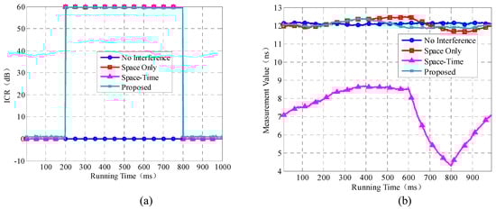
Figure 11.
Interference Cancellation Ratio (ICR) and range value in different algorithms with ideal channel. (a) ICR; (b) range value.
In Figure 11, although the ICRs of the different algorithms are almost equal, the PR measurement performance of SAP and proposed algorithm are better than that of STAP, as the PR measurement of STAP deviates from the reference and fluctuates drastically when the interference changes.
The PR measurement values were statistically analyzed, as seen in Table 3, to further compare the performance of algorithms.
Table 3.
Statistical results of ranging values (ideal channel).
As seen in Table 3, the PR measurement performance of SAP and the proposed algorithm were better than that of STAP, and the average deviation of the proposed algorithm during the whole simulation processing was 0.0673 ns from the reference.
5.5. Simulation in Non-ideal channel
In this section, the non-ideal transmission channels and antenna channels were considered. The channel model of [20] was used, and other conditions were set to be exactly the same as those of Section 5.4. The simulation results are presented in Figure 12.
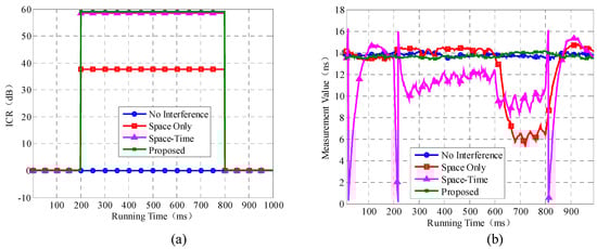
Figure 12.
ICR and range value in different algorithms with non-ideal channel. (a) ICR; (b) range value.
As seen in Figure 12, when the channel was non-ideal, the ICR of SAP, which stands for the anti-jamming ability, was lower than that of STAP and the proposed algorithm, and this is consistent with the conclusion of [17] that non-ideal channel costs the time domain degrees of freedom and deteriorates the anti-jamming performance of SAP. Moreover, as seen in Figure 12, the PR measurement of SAP deviated from the reference and fluctuated drastically, and the situation was even worse for the ranging of STAP. However, the performance of the proposed algorithm was stable without deviation, which shows that the proposed algorithm effectively mitigated the interference while introducing no bias.
Table 4 statistically analyzed the PR measurement values in the non-ideal channel to further compare the performance of algorithms.
Table 4.
Ranging performance statistics results (non-ideal channel).
As seen in Table 4, the PR measurement performance of the proposed algorithm was significantly better than that of traditional SAP and STAP, and the deviation of the proposed algorithm in different simulation steps was less than 0.4 ns. Moreover, the 1000 ms average deviation of the proposed algorithm was 0.0864 ns, compared to 1.2597 ns for SAP and 2.4353 ns for STAP. Moreover, compared to the non-jamming value of 0–200 ms, the average deviation of the proposed algorithm in the whole simulation process was about 0.0864 ns.
6. Conclusions
Antenna array processing is widely used for GNSS anti-jamming, but the traditional space–time processing will introduce deviations to the PR measurement. In this paper, the influence of STAP on pseudo-code ranging performance is analyzed. On the one hand, the delay of the space–time adaptive filter is uncertain because the space–time adaptive filter only processes the consistency of the data of each channel, and it does not have a reference delay. On the other hand, the space time filter causes uncertain distortion to the ACF as the space–time processing is similar to introducing a multipath whose characteristics are related to many factors such as the direction, power, quality of interference, and so on.
In this paper, an antenna array anti-jamming algorithm with PR measurement deviation suppression is proposed. In the proposed method, one antenna is chosen as 0 delay reference and the delay constraint for other antennas is added when generating the weights of a space–time anti-jamming filter. The simulation results show that in the testing scenarios, the PR measurement deviation of the proposed method is less than 0.5 ns without the anti-jamming performance loss. Therefore, the proposed algorithm can be used for high-precision PR measurement in antenna array anti-jamming processing.
Author Contributions
The authors confirm the contribution to the paper as follows: concept idead, desgin, software, and validation: Z.L.; concept idea, design, and supervision: F.C.; writing, original draft preparation: Y.X.; writing, review and editing: Y.S. and H.C. All authors have read and agreed to the published version of the manuscript.
Funding
This research was funded by National Natural Science Foundation of China, grant number 41604016 and 61601485.
Conflicts of Interest
The authors declare no conflict of interest.
References
- Xu, T.; Xingxing, L.; Gethin, W.R.; Craig, M.H.; Huib, d.L.; Fei, G. 1 Hz GPS satellites clock correction estimations to support high-rate dynamic PPP GPS applied on the Severn suspension bridge for deflection detection. Gps Solut. 2019, 4, 23–28. [Google Scholar]
- Hyeong-Pil, K.; Jong-Hoon, W. Analysis of ground transmitter interference range for GPS L1 signals in the ground test-bed environment of a navigation satellite system. IET Radarsonar Navig. 2019, 13, 402–409. [Google Scholar]
- Kou, Y. GPS Principles and Applications; Publishing House of Electronics Industry: Beijing, China, 2014. [Google Scholar]
- Zhao, Y.; Zhang, P.; Guo, J.; Li, X.; Wang, J.; Yang, F.; Wang, X. A New Method of High-Precision Positioning for an Indoor Pseudolite without Using the Known Point Initialization. Sensors 2018, 18, 1977. [Google Scholar] [CrossRef] [PubMed]
- Yingwei, Z. Applying Time-Differenced Carrier Phase in Non-differential GPS/IMU Tightly Coupled Navigation Systems to Improve the Position Performance. IEEE Trans. Veh. Technol. 2017, 66, 992–1003. [Google Scholar]
- Cillian, O.D.; Marco, R.; Daniele, B.; Duaardo, C.; Eduardo, C.; Joaquim, F.; Fréderic, B.; Dominic, H. Compatibility Analysis between LightSquared Signals and L1/E1 GNSS Reception. In Proceedings of the 2012 IEEE/ION Position, Location and Navigation Symposium, Myrtle Beach, SC, USA, 23–26 April 2012; pp. 447–454. [Google Scholar]
- Jang, J.; Seo, S.; Ahn, W.G.; Lee, J.; Park, J. Performance analysis of an interference cancellation technique for radio navigation. IET Radarsonar Navig. 2018, 12, 426–432. [Google Scholar] [CrossRef]
- Fante, R.L.; Vaccaro, J.J. Wideband Cancellation of Interference in a GPS Receive Array. IEEE Trans. Aerosp. Electron. Syst. 2000, 36, 549–564. [Google Scholar] [CrossRef]
- Rezazadeh, N.; Shafai, L. A Compact Microstrip Patch Antenna for Civilian GPS Interference Mitigation. IEEE Antennas Wirel. Propag. Lett. 2018, 17, 381–384. [Google Scholar] [CrossRef]
- Dai, X.; Nie, J.; Chen, F.; Ou, G. Distortionless space-time adaptive processor based on MVDR Beamformer for GNSS receiver. IET Radar Sonar Navig. 2017, 11, 1488–1494. [Google Scholar] [CrossRef]
- Rife, J.; Khanafseh, S.; Pullen, S. Navigation, interference suppression, and fault monitoring in the sea-based joint precision approach and landing system. Proc. IEEE 2009, 96, 1958–1975. [Google Scholar] [CrossRef]
- Kim, U.S.; Lorenzo, D.S.D.; Akos, D.; Gautier, J.; Enge, P.; Orr, J. Precise Phase Calibration of a Controlled Reception Pattern GPS Antenna for JPALS. In Proceedings of the PLANS 2004: Position Location and Navigation Symposium, Monterey, CA, USA, 26–29 April 2004; pp. 478–485. [Google Scholar]
- Lee, J.; Pullen, S.; Datta-Barua, S.; Lee, J. Real-Time Ionospheric Threat Adaptation Using a Space Weather Prediction for GNSS-Based Aircraft Landing Systems. IEEE Trans. Intell. Transp. Syst. 2017, 18, 1752–1761. [Google Scholar] [CrossRef]
- Daneshmand, S.; Sokhandan, N.; Zaeri-Amirani, M.; Lachapelle, G. Precise calibration of a GNSS antenna arrays for adaptive beamforming applications. Sensors 2014, 14, 9669–9691. [Google Scholar] [CrossRef] [PubMed]
- O’Brien, A.J.; Gupta, I.J. Mitigation of Adaptive Antenna Included Bias Errors in GNSS Receivers. IEEE Trans. Aerosp. Electron. Syst. 2011, 47, 524–538. [Google Scholar] [CrossRef]
- Church, C.M.; Gupta, I.J.; O’Brien, A.J. Adaptive antenna induced biases in GNSS receivers. In Proceedings of the ION 63rd Annual Meetings, Cambridge, MA, USA, 23–25 Apirl 2007; pp. 204–212. [Google Scholar]
- Zukun, L.; Junwei, N.; Feiqiang, C.; Huaming, C.; Gang, O. Adaptive Time-taps of STAP under Channel Mismatch for GNSS Antenna Arrays. IEEE Trans. Instrum. Meas. 2017, 66, 2813–2824. [Google Scholar]
- Church, C. Estimation of Adaptive Antenna Induced Phase Biases in Global Navigation Satellite Systems Receiver Measurements; The Ohio State University: Columbus, OH, USA, 2009. [Google Scholar]
- Kim, U.S.; Lorenzo, D.S.; Gautier, J. Phase effects analysis of patch antenna CRPAs for JPALS. In Proceedings of the 17th International Technical Meeting of the Satellite Division of The Institute of Navigation (ION GNSS 2004), Long Beach, CA, USA, 21–24 September 2004. [Google Scholar]
- Zukun, L.; Junwei, N.; Feiqiang, C.; Gang, O. Impact on Anti-jamming Performance of Channel Mismatch in GNSS Antenna Arrays Receivers. Int. J. Antennas Propag. 2016, 2016, 1–9. [Google Scholar]
- Zukun, L.; Junwei, N.; Youda, W.; Gang, O. Optimal Reference Element for Interference Suppression in GNSS Antenna Arrays under Channel Mismatch. IET Radarsonar Navig. 2017, 11, 1161–1169. [Google Scholar]
- Compton, R.T. The Power-Inversion Adaptive Array: Concept and Performance. IEEE Trans. Aerosp. Electron. Syst. 1979, 15, 803–814. [Google Scholar] [CrossRef]
- Zukun, L.; Huaming, C.; Feiqiang, C.; Junwei, N.; Gang, O. Blind Adaptive Channel Mismatch Equalization Method for GNSS Antenna Arrays. IET Radarsonar Navig. 2018, 12, 383–389. [Google Scholar]
- Feiqiang, C.; Junwei, N.; Baiyu, L.; Wang, F. Distortionless space-time adaptive processor for global navigation satellite system receiver. Electron. Lett. 2015, 51, 2138–2139. [Google Scholar]


© 2020 by the authors. Licensee MDPI, Basel, Switzerland. This article is an open access article distributed under the terms and conditions of the Creative Commons Attribution (CC BY) license (http://creativecommons.org/licenses/by/4.0/).