Rating the Participation in Demand Response Programs for a More Accurate Aggregated Schedule of Consumers after Enrolment Period

Abstract

Aggregation of small size consumers and Distributed Generation (DG) units have a considerable impact to catch the full flexibility potential, in the context of Demand Response programs. New incentive mechanisms are needed to remunerate consumers adequately and to recognize the ones that have more reliable participation. The authors propose an innovative approach to be used in the operation phase, to deal with the uncertainty to Demand Response events, where a certain target is requested for an energy community managed by the Aggregator. The innovative content deals with assigning and updating a Reliability Rate to each consumer according to the actual response in a reduction request. Three distinct methods have been implemented and compared. The initial rates assigned according to participation in the Demand Response events after one month of the enrolment period and the ones with higher reliability follow scheduling, performed using linear optimization. The results prove that using the proposed approach, the energy community manager finds the more reliable consumers in each period, and the reduction target achieved in DR events. A clustering algorithm is implemented to determine the final consumer rate for one month considering the centroid value.

1. Introduction

The energy sector is facing challenges due to the need for more efficiency in energy usage. More reliable and efficient energy networks and markets are desired, empowering players, enabling bidirectional communication, and finding solutions to replace fossil fuels [1,2,3]. Demand Response (DR) concept is one of the main topics in the literature due to the potential benefits and to the search to overtake the barriers and achieve successful implementation in the energy market.

1.1. Background and Motivation

Directive 2019/944 [4] defines DR as "the change of electricity load by final customers from their normal or current consumption patterns in response to market signals, including in response to time-variable electricity prices or incentive payments, or in response to the acceptance of the final customer’s bid to dell demand reduction or increase at a price in an organized market". This directive’s primary goal will be finding a way to overcome existing obstacles to the completion of the internal electricity market. Directive 2003/54/EC and Directive 2009/72/EC contributed to the conception of the electricity market as it is currently but, with these new challenges coming from Smart Grids concept introduction, several updates must be done, namely regarding the consumers’ role [5,6]. With Directive 2019/944, considering that to achieve the main goals with effectiveness, the innovation must be incentivized, and the flexibility compensated. Only after a fully functional energy market, the possibility of adding renewable energy to the actual grid, ready to deal with the uncertainties associated, can become a reality taking a new step to decarbonize the system.

Currently, and in the context of the work in this paper, the main stakeholders involved in the flexibility markets are Transmission System Operator (TSO), Distribution System Operators (DSO), Balance Responsible Parties (BRPs), Aggregator, and Retailer. TSO is responsible for the service and stability of the transmission system. Regarding DSO, it is the entity responsible for the operation of the distribution system and the power delivery to customers. The BRP role can be played by a market entity (such as wholesale supplier or retailer), or its chosen representative responsible, in charge of dealing with imbalances, paying penalties for deviations from energy schedules. Finally, the Retailer is an existing commercial entity selling electrical energy to consumers.

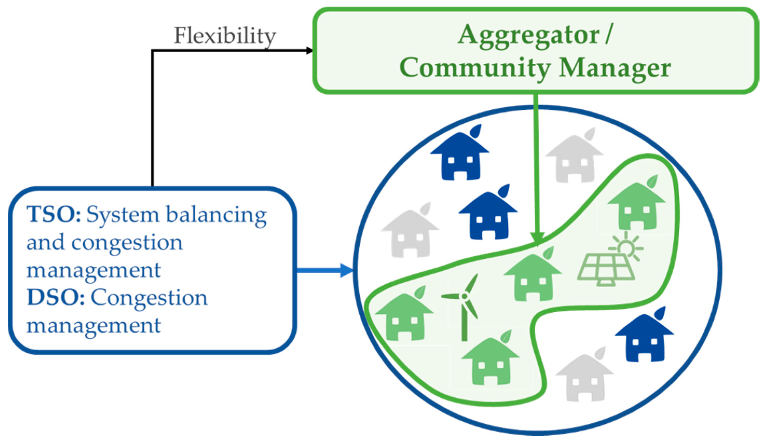
Regarding the role of the Aggregator in a local community, it depends on the market model. Still, this entity can operate in different parts of the network and use the associated resources for trading electricity and ancillary service markets. The Aggregator can also act as an intermediary for the transactions between small entities, such as consumers, and the wholesale market so it is the entity that accumulates flexibility through renewable-based generation and consumers (through DR), as Figure 1 presents. In the present paper, the Aggregator acts as a Local Energy Community (LEC) manager. In [7], LEC is defined as “an association, a cooperative, a partnership, a non-profit organization or other legal entity which is effectively controlled by local shareholders or members, generally, value- rather than profit-driven, involved in distributed generation and performing activities of a distribution system operator, supplier or aggregator at local level, including across borders”. Many benefits were previewed from this concept, namely regarding the relationship between the DSO and the communities: DSO is now allowed to manage some of the difficulties associated with the local generation (e.g., by controlling local flexibility resources) which could drastically reduce the network costs.

The consumers’ role in this market, although currently less explored and with increasing value, becomes crucial to achieving the required level of flexibility to adjust the current network to recognize a distributed, renewable, and volatile generation [8,9]. Currently, consumers do not have the right tools to access information about their consumption, in real-time or near to real-time, to actively participate in the energy market. Still, consumers are more conscious and worried with climate issues; aware of their capabilities as an active role; searching for the investment in Distributed Generation (DG), for instance in their houses; finding mechanisms to consume in a more clean, efficient, and economical way through DR [10,11].

Therefore, the creation of new players and business models developed to deal with this "new type" of players must exist, considering that not all the consumers have the same behaviour causing uncertainties to the management of the market. Services that produce benefits to only a particular group of the population may bring negative results. In this way, the consumers’ characterization and behaviour study is crucial. The referred challenges are the primary motivation for the present work. As already mentioned, being the Aggregator of the entity capable of managing a local energy community, providing the right tools to be successful. However, this entity must have reliable information about the resources to decide which one should participate in the eventuality of a DR event to avoid imbalances. The goal is to create a tool able to answer questions such as: Should the Aggregator rely on all the consumers in the community? If not, is it possible to differentiate them? How? When in a DR event, the consumers who reduce accordingly should they compensate differently? And those who do not answer?

The authors of the present paper designed a methodology that deals with the uncertainty of the small resources, focusing on the consumers with the assignment of a Reliability Rate to optimally manage the local community in cases of DR events. Previous works [12,13,14] already proposed a business model to help Aggregators, although the doubt associated with the actual response of the consumers was never considered. The action described in the paper is relevant to the operation being a simulation of a real-time reaction by the resources to DR events and how the Aggregator should manage the uncertainties associated.

1.2. Related Literature

The related literature presents distinct approaches to solve the scheduling problem when dealing with the introduction of demand-side in the energy market and how the load diagram can influence network reliability. Muhsen et al. [15] proposed a multi-objective optimization differential evolution method to solve the load scheduling problem in terms of cost and energy saving, creating a set of optimal solutions. Ilo et al. [16] considered a holistic power system architecture that gathers the relevant components in a single structure focusing on the decarbonization of the sector cost-effectively while guaranteeing data privacy and safety against external threats. Li, Dou, and Xu [17] used a firefly optimization algorithm to solve the scheduling problem of a distribution network. The simulation, prediction of the load, travel chain of electric vehicles, and different charging methods were considered to establish a predictive model, and the establishment of demand response sideload. Khalid et al. [18] presented a pricing model to delineate the rates for on-peak and shoulder-peak hours having the goal of charging a per-unit price—taking into account the consumed energy and the extra generation cost. Faria and Vale [19] proposed a method to minimize the operation costs, where the virtual power player manages DR programs and respects the consumption shifting constraints making a comparison between the advantages of DR use and DG. Proving the benefits of DR in the operation of distributed energy resources, namely when considering the lack of supply. Hu, Lu, and Chen [20] formulated a stochastic multi-objective Nash–Cournot competition model to simulate DR in an uncertain energy market. The authors considered that DR programs can reduce peak energy consumption, energy price, and carbon dioxide emissions. The lack of studies connecting the uncertainty and the actual response of the consumer in the scheduling is visible. However, these works prove the increasing influence of this new player in the transactions of the energy market.

The comprehension of the consumer’s behaviour is a significant study as their decision power is higher, and they may become the focal point of this sector. Nicholas Good [21] presented research on the suitability of behavioural economics as an approach for modelling demand response. This author reminds us that most of the studies shaped under the demand response topic assume that the end-user is always rational and an active economic agent. In this way, its concluded from this study that centrally coordinated actions may produce the best results since consumers are willing to collaborate and sacrifice thermal comfort without compensation to achieve a common objective—secure operation of the local electricity network. Ruiz et al. [22] contradicting the previous conclusion, presented a bottom-up approach based on physical end-use load models. These authors study the individual responses of combining a random sample of customers building an aggregated load Demand Response model by performing a simulation of the different reactions with an optimization algorithm based on mixed-integer linear programming. It proved that minimizing the electricity bill occurs while maintaining the consumer’s comfort level. The results from this study show that the higher the incentive offered by the Aggregator (disagreeing with [21] which believed in the insignificance of compensation for this kind of discomfort), obtain higher load reductions with this approach. Both [21,22] agree, as well as the authors of the present paper that consumers must be willing to participate in the DSM programs. They must also allow the application of more restrictive control actions, over their controllable appliances, although this implies higher losses on their comfort level. However, the authors of the present paper consider it essential to compensate them, incentivizing continuous participation in the management of the local community.

There is a necessity to find techniques to incentivize and support the participation of the small resources to decrease the uncertainty associated with them. Monfared and Ghasemi [23] proposed a value-based hourly pricing approach, concluding that the value of the electricity is not the same to end-users depending on the benefits for each consumer. The objective of the proposed methodology was to improve the effectiveness of price-based Demand Response programs implemented in a smart distribution network. Jiang et al. [24] developed a method to deal with performance and efficiency uncertainties from distributed energy resources. These authors formulate a scenario-based two-stage algorithm to solve the problem, preserving the multiple risks in the entire decision-making process. Khan et al. [25] designed a knowledge-based system for short-term load forecasting where the precision is improved by a different priority index to select similar days.

1.3. Innovations and Contributions

The proposed methodology provides innovative contributions in the field of consumers’ response uncertainty, which is a complicated matter. With the novel approach proposed, after the enrolment period, the Aggregator will be able to identify and schedule reliable consumers to participate in DR events, increasing the accuracy and dealing with the doubt. The main goal of the present paper is to provide essential means and knowledge to the entity that manages the LEC to be successful in DR implementation and use. It is critical to understand what extent each consumer can contribute to DR and be more reliable, in each period of the day. In this way, the community manager can appropriately reward the consumer for the discomfort caused by DR events. The following features are listed as innovative aspects of the methodology proposed in the present paper:

• Consider the consumer behaviour from past DR events, during a full month period as the enrolment period;
• Categorize the consumers according to their actual response;
• Remunerate the consumers according to their actual response;
• DR events with DR targets for the community being essential to understand in which consumers the Aggregator can rely on to achieve the goals;
• Collaboration between members of the community regarding local balance, highlighting the importance of the role of the prosumer and the influence of prioritizing the local generation to suppress the demand;
• Comparison between the requested reduction and the actual reduction when on DR event, being a crucial factor to increase or decrease the reliability rate;
• Interactions from the consumers’ side to improve the reliability rate, either through higher reductions or with lower tariffs;
• Incentives, through remuneration, according to the reliability rate group inserted;
• Identify the monthly reliability rate of a consumer.

According to the actual response for DR events, in different temporal ranges, a reliability rate is assigned to each consumer. This rate was calculated through three independent rates. The way of using the reliability rate through the proposed methodology depends on three methods: Basic Rate Method, Cost Rate Method, and Clustering Rate Method.

After this introduction, Section 1 presents several related works and the comparison with the proposed methodology detailed in Section 2—Materials and Methods, as well as the case study. Section 3 presents the scenarios selected, the results obtained by the application of the proposed approach to show the feasibility of the methodology and the respective discussion. Finally, Section 4 brings the conclusions from this study.

2. Materials and Methods

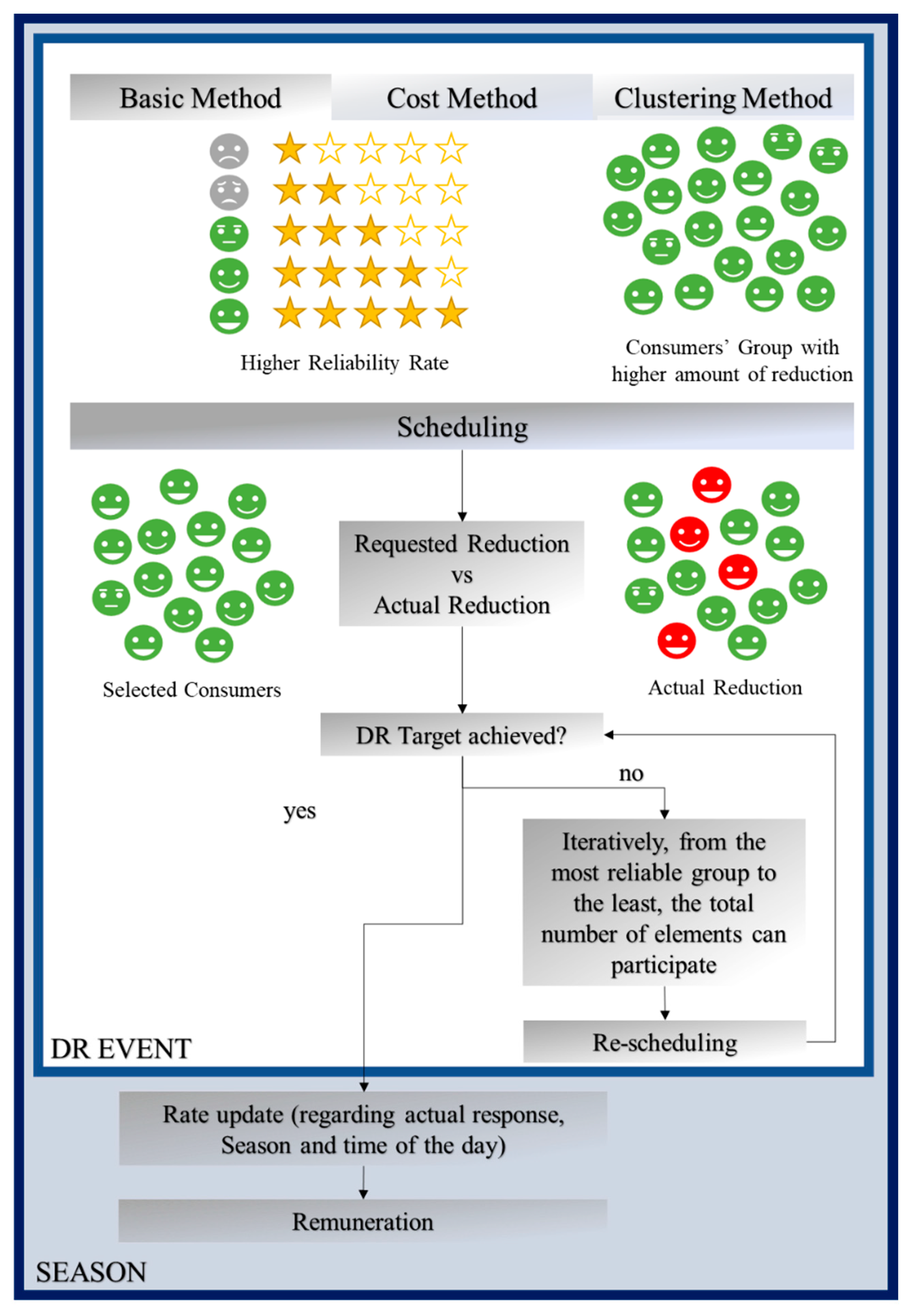
The authors implemented a methodology that gives the Aggregator, as the entity that manages the energy community, a tool to optimally manage the resources associated and have some knowledge about their reliability when participating in DR events. With this, Figure 1 shows the proposed methodology. Presenting three approaches—Basic Rate Method, Cost Rate Method, and Clustering Rate Method, and each one deals with the uncertainty of the consumer differently. These methods are applied per DR event and can be used in different contexts, namely different seasons, as the consumers’ behaviours change through the year.

In the Basic Rate Method, the selection phase considers only consumers with values higher than the nominated minimum for scheduling, i.e., for example in Figure 2 consumers with more than three “stars”, were represented as green faces, chosen to participate in DR event. The initial reliability rate considers two independent rates: Historical Rate (HR) and the Last Day Rate (LDR). The first one takes into account past information from the consumer. The second considers the reliability rate assigned to the consumer in the same period of the previous day. The Aggregator schedules its resources considering a DR target for this community. After, a comparison is made between the actual response and the requested one. In the hypothesis of not achieving the DR target in a first schedule, a re-schedule considering the remaining consumers with DR contracts is performed, allowing their reliability rate to increase by participating in the management of the local community.

The update of the final reliability rate of each consumer considers more than one independent rate related to the actual response. Although Cut-Rate (CR) has some percentage in the formulation, a higher reduction than the requested may not be enough to increase their rate. The other two, HR and LDR, have also weight in the formulation of the final reliability rate of a consumer to control the rate change speed.

In the case of the Cost Rate Method, a feature is added when updating the final reliability rate: The price also fluctuates. The entire process is similar to the primary method but introduces a new strategy for the consumer. They can change their reliability prices to increase their rates. In other words, when each group of resources is called to participate in a DR event, the ones with lower prices are selected (considering minimization of operational costs regarding the Aggregator). If the actual response surpasses the expectations, the possibilities of increasing the final reliability rate arises. The third and final approach is formulated based on clustering: The idea is to compare with the Basic Rate Method. Let’s call it the Clustering Rate Method. Mainly, the consumers are also classified by reliability rate and only the ones with a higher rate will be considered in the scheduling. However, an adaptation is considered using clustering: Only the consumers with higher values of contracted reduction are considered for the first scheduling. That is, each rate will be clustered, and the group with the higher sum of pledged reduction follows to the next phase. The remaining process stays the same.

Regarding the scheduling phase, a linear optimization is performed to minimize operation cost from the perspective of Aggregator. The scheduling input needs several parameters, and it is the responsibility of the Aggregator to gather them all to schedule all the associated resources successfully. Information such as the maximum capacity of the DG units, the external suppliers, and the reduction capacity of the consumers belonging to DR programs, as well as the consumption tariffs associated with each resource is needed. The authors considered the existence of two types of external suppliers: Regular and additional.

Equation (1) introduces the objective function of the problem:

Min OS = ∑ [P_DG (p, t) C_DG (p, t)] + ∑ [P_IDR (c, t) C_IDR (c, t)] + ∑ [P_SUPA (sa, t) C_SUPA (sa, t)]
+ ∑ [P_SUPR (sr, t) C_SUPR (sr, t)] + P_NSP(t) C_NSP (t)

(1)

The optimal scheduling is done for each period t and the different resources in the local community such as DG units (P_DG), consumers belonging to DR programs (P_IDR) and suppliers, both regular (P_SUPR) and additional (P_SUPA) are considered. The external suppliers are only applied in the case of DG units that were not able to suppress the total amount of consumption to achieve the network balance, as presented in Equation (2):

∑ [P^initial (c, t) − P_IDR (c, t)] = ∑ [P_DG (p, t)] + ∑ [P_SUPA (sa, t)] + ∑ [P_SUPR (sr, t)] + P_NSP(t)

(2)

This equation is essential and a complex problem for the network operators. The goal is to maintain the value of Non-Supplied Power (NSP)—the amount of demand not satisfied, null proving that the network is being optimally managed. In this way, several options to fulfil the demand (P^initial) requests are available: DG units and external suppliers are also included in the production side, and DR events are also considered.

Other restrictions were added to the presented optimization: Regarding the consumers who participate in DR events Equation (3) and Equation (4) control, their participation and Equation (5) and Equation (6) defines the DR target for the community. When compared with previous works from the authors, Equations (4)–(6) are an innovation.

The proposed method, as shown in Figure 2, includes a possible rescheduling with all the consumers in the impossibility of the actual response from the selected were not enough to achieve the DR target in the first stage. Giving this, the ones chosen in the scheduling should maintain the requested reduction—considered as the new P_IDR^Min in Equation (4), and only be added to the difference needed being the value of the first scheduling considered as DRtarget^min in Equation (6):

P_IDR (c, t) ≤ P_IDR^Max (c, t)

(3)

P_IDR (c, t) ≥ P_IDR^Min (c, t)

(4)

∑ [P_IDR (c, t)] ≤ DRtarget^Max (c, t)

(5)

∑ [P_IDR (c, t)] ≥ DRtarget^Min (c, t)

(6)

Regarding the distributed generation resources in the local community, they are restricted by Equations (7)–(9). Equation (7) represents the upper bound, considering the maximum capacity and Equation (8) the lower bound. The lower bound was considered for specific cases such as type wind units, which must be constrained by the resulting power from the cut-in and cut-out wind. Equation (9) gives the Aggregator more control when using the generation, restricting the amount that can be used. A similar tactic used for external suppliers:

P_DG (p, t) ≤ P_DG^Max (p, t)

(7)

P_DG (p, t) ≥ P_DG^Min (p, t)

(8)

∑ [P_DG (p, t)] ≤ P_DG^Total (p, t)

(9)

The constraints related to external suppliers are presented from Equation (10) to Equation (13). The upper bound is established by Equation (10) for additional suppliers and Equation (12) for regular suppliers. Equation (11) and Equation (13), as in DG units, restrict the total amount of generation from this source:

P_SUPA (sa, t) ≤ P_SUPA (sa, t)

(10)

∑ [P_SUPA (sa, t)] ≤ P_SUPA (t)

(11)

P_SUPR (sr, t) ≤ P_SUPR (sr, t)

(12)

∑ [P_SUPR (sr, t) ≤ P_SUPR (t)

(13)

After DR target is achieved for the DR event, there is the update of the reliability rate and the remuneration for the participants. The remuneration is considered as an incentive and done according to tariffs existing in the same reliability rate. For the three methods, the reliability rate update is the same: Considering HR, LDR, and CR in the formulation. However, for the Cost Rate Method, the consumers that were not selected for the DR event can change their cost in DR events to be selected.

As soon as the three approaches are compared, a final study is done. The authors propose to find the proper reliability rate per consumer per month, using a clustering method. The task of the clustering object is created from the need of the human to define prominent attributes and identify them as a type. Therefore, several disciplines use this method—from mathematics to biology, the goal is the same: Establishing categories for the objects and assigning individuals to the proper groups within it [26]. In this way, the selected method for the first study is a well-known partitioning clustering method: K-means. The algorithm consists in finding, iteratively, the value that represents each group—centroid. The centroid element is found when the distance between itself and the remaining is minimal. Several techniques are applied to calculate the gap, namely Euclidean distance. The results for one month will be considered, and the consumers will be represented by one reliability rate only.

The proposed methodology was studied resorting to a database formed by a real distribution network, with ten random local communities and a total of 20,310 consumers from five different types classified as Domestic, Small Commerce, Medium Commerce, Large Commerce, and Industrial. Although the consumers are the focus of this work, for the scheduling phase, the generation units were also considered in this study, highlighting Distributed Generation (DG) units, namely Small Hydro, Waste-to-energy, Wind, Photovoltaic, Biomass, Fuel Cell, and Co-generation.

Table 1. Small resources characterization in the ten communities.

CONSUMPTION
Type	Domestic	Small Commerce		Medium Commerce	Large Commerce	Industrial
# elements	10,168	9828		82	85	147
Energy (kWh)	9369.35	7983.35		11,254.75	10,880.48	23,142.48
Max Load Reduction (kW)	4684.7	3991.7		15,756.7	9792.4	20,828.2
Initial Price (m.u./kWh)	0.12	0.18		0.20	0.19	0.15
GENERATION
Type	Small Hydro	Waste-to-Energy	Wind	Photovoltaic	Biomass	Fuel Cell	CHP
# elements	25	7	254	208	25	13	16
Energy (kWh)	214.05	53.10	5866.09	7061.28	2826.57	2457.60	6910.10
Tariff (m.u./kWh)	0.0961	0.0900	0.0988	0.2889	0.1206	0.0945	0.0975

presents the characterization of all consumers and generation units in the ten local communities.

One month of information was considered for the present study. The whole database, consumption, and generation are divided into periods of 15 min, so a day has 96 periods where the first one is at 12 am and 96 is at 12 pm. The chosen historical information used for the creation of scenarios was April 2018. In this way, the database has 2880 periods.

The present study focuses on the reliability of each consumer when requested to participate in DR events. The Aggregator of the local community has DR targets according to the period of the day, and it is expected that consumers with higher reliability rate answer as requested. In the present scenarios, it was considered a DR target of 100 kW for each type of event.

For the three proposed methods, the techniques to calculate the initial and final reliability rate is different and can influence other variables—namely in the Cost Rate Method where the consumers change their cost to be considered in the scheduling. Both initial and final reliability rates have a value between 1 and 5. They are dependent on the consumers’ performances in DR events for different periods where independent rates were attributed as

Table 2. Independent rates weights.

	HR	CR	LDR
Initial	0.4	-	0.6
Final	0.33	0.33	0.33

. A Historical Rate (HR) to past information with more than one day; the Previous Day Result Rate in the same period (LDR), and the Actual Reduction Rate for the studied period (CR).

According to the stage of the method, the weights of these independent rates in the formation of the reliability rate are different. In this way, Table 2 presents the masses considered in the present case study.

3. Results and Discussion

The current section shows a comparison between three methods and the analysis done to understand the behaviour of the consumers over a month regarding the uncertainty of their participation in the management of the community.

Considering 96 periods in a day, to perform scheduling for one period, the solving time for the community as a whole is overly high to be used in a real-time situation, not considering the remaining process. Giving this, the authors opt for presenting the study only for one community: The one with a higher reliability rate, being this one the centre of the case study. In this way,

Table 3. Average rates from the local communities.

Community	1	2	3	4	5	6	7	8	9	10
Number of Elements	2501	658	3480	406	4982	1598	398	3789	1509	989
Average Rate	2.97	3.03	2.99	3.10	3.01	3.03	2.94	3.01	3.00	2.98

presents a survey of the average rate found in the communities and the one with higher value was considered.

Section 3 is subdivided into five subsections. Firstly, the results from each method which represent three subsections. After, a study of Consumer Reliability Rate Identification for the Month—k-means—where a clustering method is used to assign a reliability month rate for each consumer. Finally, a survey on Reliability Rates over different seasons. The steps taken in the first three subsections are presented in

Table 4. Study steps and criteria to compare the three methods.

	Basic Rate Method (Section 3.1)	Cost Rate Method (Section 3.2)	Clustering Rate Method (Section 3.3)
Consumer Selection by Initial Rate (Sub-section 3.X.1.)	Rate ≥ 3	Rate ≥ 3	Rate ≥ 3 and The group with higher reduction according to the clustering method
Scheduling and Re-Scheduling (Sub-section 3.X.2)	Until achieving the target in a DR event (comparison between how quick the goal can be achieved by understanding the quality of the selected samples—the more reliable consumers)
Rate Update (Sub-section 3.X.3)	Actual reduction vs. Requested Reduction	Actual reduction vs. Requested Reduction and Cost Update	Actual reduction vs. Requested Reduction
Remuneration (Sub-section 3.X.3)	Maximum tariff per rate (final minimum reward in the perspective of the Aggregator)

, as well as the criteria used to compare them. Moreover, in the same table, there is a correspondence between the subsections and the steps taken to clarify the structure of the present section.

In the analysis of the results from the three methods, there are three parts. The first one, Initial Rate, the initial number of elements per period and per group is presented. The Scheduling and Re-scheduling Results, showing the requested and the actual reduction through the month. Finally, Rate Update and Remuneration, where the final reliability rates and the remuneration are presented analyzing per period.

3.1. Basic Rate Method

The Basic Rate Method consists of only selecting the higher reliability rate consumers to the scheduling. Regarding the update of the final reliability rate for each period, considering the three independent rates and the cost associated with the DR events is not revised. Since it is the first method to be analyzed, a more detailed view of the results is done. As mentioned, April 2018 was selected, and the DR events are exhibited in

Table 5. DR (Demand Response) events.

Day	Event 1 (11:00–12:00)	Event 2 (18:00–19:00)
Sunday, 1	x	-
Thursday, 4	x	-
Saturday, 7	x	-
Tuesday, 10	-	x
Friday, 13	-	x
Monday, 16	-	x
Thursday, 19	x	-
Sunday, 22	-	x
Wednesday, 25	-	x
Saturday, 28	x	-

. As can be seen, two types of events are considered: Event 1 is between 11 am–12 am, and Event 2 is between 6 pm and 7 pm. The frequency of each occurrence in this month is five, having been performed ten events in this study.

3.1.1. Initial Reliability Rate

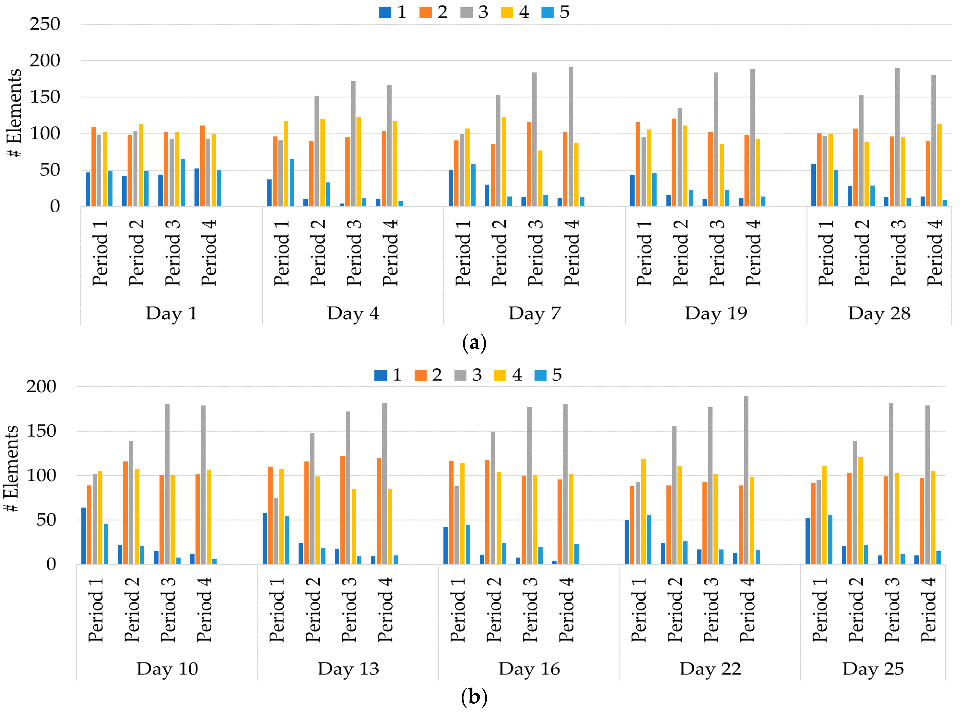
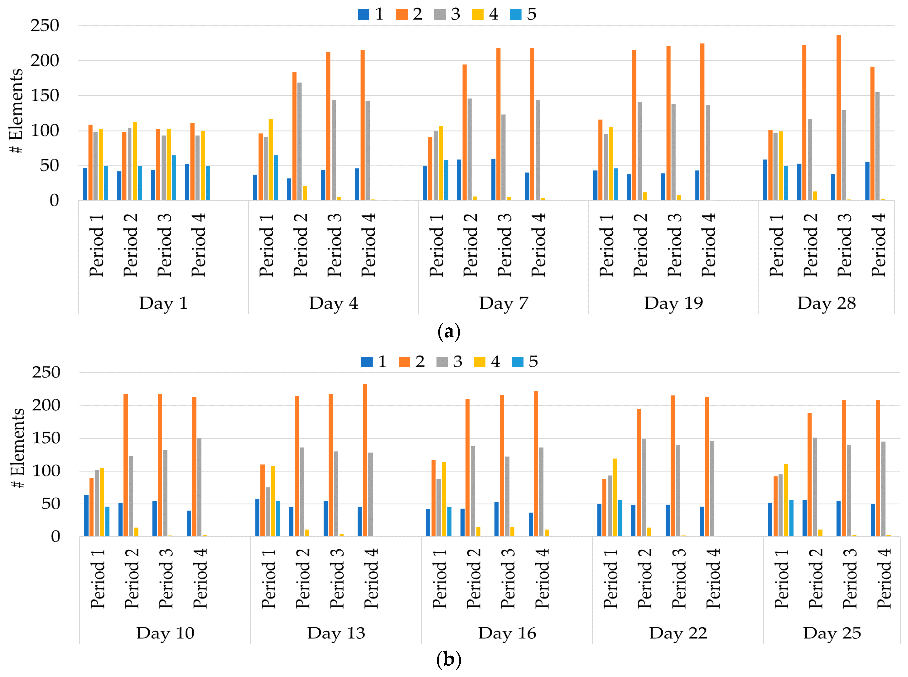
The Initial Reliability Rate considers the HR and the LDR, finding that Day 1 does not have LDR, and the Initial Reliability Rate is equal to the HR. Figure 3 shows the number of elements per group in each event day. Each event has four periods—15 min each.

Initially, on the first day of the month, a DR event between 11 am and 12 am happened. For the DR event, in Period 1 only 250 were able to participate; for Period 2 the value increased to 266; for Period 3 and Period 4 the value decreased to 260 and 243, respectively.

For the following days, the actual response in the previous day was impacted by LDR.

Day 4 also had an event between 11 am and 12 am. The Reliability Rate 4 had the highest number of elements in all the periods, counting with 167 in the last one. In this second day of Event 1, more consumers were able to participate: In Period 1 the total was 273, Period 2 was 305, Period 3 was 307 and, finally, Period 4 was the one with the lower number of elements, 292.

On Day 7, Event 1 also occurred. The number of consumers able to participate in Period 1 was 265; in Period 2 were 290; in Period 3 decreased to 277, and in the final period of the event 291 consumers were able to participate. On the third day of Event 1, Reliability Rate 3 had the highest number of elements over time.

On Day 10, the DR event occurred between 6 pm and 7 pm. For the first event of this genre, the HR was the only rate considered in this Initial Rate. For Period 1, there were 253 elements capable of participating in the scheduling; in Period 2, 15 elements were added; Period 3 increased to 22 elements and, finally, for Period 4 the number of elements reached 292.

Day 13 had an Event 2, similar to the previous day. The number of elements in Reliability Rate 1 decreased from 58 to 9 at the end of the DR event. Reliability Rate 2 increased ten elements comparing the initial and the final period. Reliability Rate 3 doubled the number of elements. Regarding Reliability Rate 4 elements, it decreased the number of elements from 108 to 85. Reliability Rate 5 also had a relative decrease in the number of elements comparing the beginning and the end of the event (−82%). Day 16 was also one of the Event 2 days. The third event of this type counted with 247 consumers in the first period of the event, 277 in the second, 298 in the third, and 306 in the final.

Regarding Day 19 from the study month, an event between 11 am and 12 am occurred, being the fourth of Event 1 type. At the beginning of the event, 247 consumers were available to participate. For the following periods, this number increased to 22, 46, and 49 elements.

The final two events from type 2 happened on Day 22 and Day 25. The number of elements increased over time for both situations, with 304 and 299 elements, respectively, being able to participate at the end of the event.

The last event of the studied month was type 1, as can be seen in Table 4. Both Reliability Rate 1 and Reliability Rate 5 decreased the number of elements over time, meaning that consumers’ rates were updated to the groups in-between. In this case, the Reliability Rate 3 had the highest number of elements in the final period of the event, and through Event 1 it was possible to notice the impact from the last day in the number of elements per period. In Period 1, when comparing the number of elements in the first day of this type of event with the last one, the total of elements able to participate decreased by 1.60%. Regarding Period 2, the number of elements increased by 1.8%. For Period 3, the impact was higher than the previous ones, increasing by 14.23%. However, Period 4 was the one with a more significant difference (24.28%).

Now, Event 2 had a distinct outcome since the percentual difference between the number of elements in the first day of this type of event (per period) and with the last one did not reach 5% in all periods. Comparing with the other occasion, maybe this period of the day brings more discomfort to the consumers and less are willing to reduce their consumption.

3.1.2. Scheduling and Re-Scheduling Results

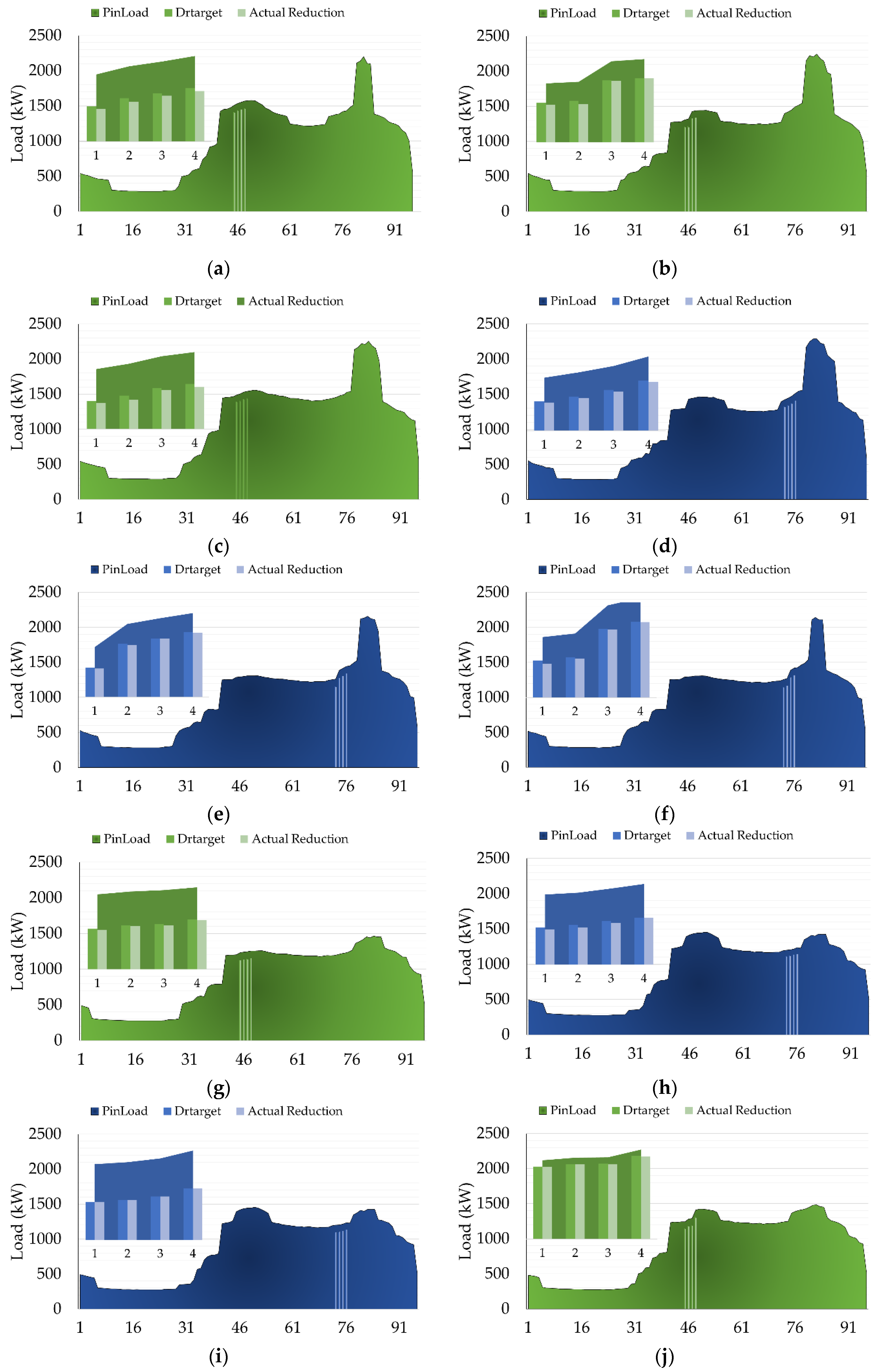
In this subsection, the results from the scheduling of the local community according to the method are presented. This method considers that all consumers with reliability rates above the nominated minimum are convoked. Still, the proposed optimization will decide which of those are selected to achieve the DR target for the events. Figure 4 shows the initial load curve for the event days (darker colour) and the values of the DR target (medium colour) and actual reduction (lighter colour) from each period. A more comprehensive chart of the DR event is also presented. Moreover, different colours were applied to ease the distinction between the type of events: One is green, and two is blue.

In the Day 1 period of the DR event, the initial load floated between 1510 and 1568 kW, with the DR target of 100 kW being achieved in all the events: Period 1 with 1402 kW; Period 2 with 1425 kW; Period 3 with 1444 kW, and Period 4 with 1459 kW. For Day 4, the initial load curve had a more significant difference between the initial and the final period of the event (1309 and 1437 kW). The actual reduction was always above the DR target—highlighting Period 1 and Period 2, where this value was more than 10 kW higher than the expected. In Day 7, the actual reduction was also above the target passing the load curve from 1489 to 1382 kW in Period 1; from 1506 to 1392 kW in Period 2; from 1529 to 1423 kW in Period 3, and from 1542 to 1432 kW in Period 4.

Between 6 pm and 7 pm on Day 10, the initial load curve increased from 1423 to 1511 kW. In this event, the DR target is achieved, and the maximum actual reduction reached 8 kW higher than the expected. Regarding Day 13, the initial load curve, at the beginning of the event had, for Period 1, 1263 kW and reached 1151 kW with the actual reduction. Regarding Period 2, decreased from 1385 to 1274 kW; Period 3 started with 1415 kW and finished with 1308 kW and, finally, for Period 4 the actual reduction were reduced from 1442 to 1339 kW. As can be seen in Figure 4f, the DR target was achieved in all periods of the event for Day 16—the maximum reduction that was completed in the first period of the event decreased the initial load from 1254 to 1142 kW.

Day 19 returns to the type 1 DR event, with the DR target being also accomplished. For Period 1 the initial load was 1232 kW, and 110 kW were reduced; Period 2 started with 1240 kW and were reduced to 106 kW; Period 3 initially had 1245 kW where 110 kW were reduced; in Period 4, 101 kW were reduced from 1254 kW.

Day 22 and Day 25 had the same type of event (1), and the actual reduction was higher than the DR, not reaching 10 kW higher than the denominated value of DR target.

The last Event 2, Day 28, the actual reduction for Period 1 was 106 kW; for Period 2 was 104 kW; for Period 3 was 107, and for Period 4 was 111 kW.

Through this stage of the study and with Method 1, the Aggregator was able to select the proper consumers initially—the ones able to reduce the DR target in the Scheduling phase being not needed to resort to a Re-scheduling in the following days: Day 13, Day 16, Day 28 resorted to Re-scheduling in Period 2 and Period 4. For Day 1 and Day 19, the opposite situation happened (Re-scheduling for Period 1 and Period 3). In Day 4, Day 22, and Day 25, the Scheduling was enough to achieve the DR target for Period 3, Period 2, and Period 4, respectively. Day 7 was the only one where all the periods from the DR event needed a Re-scheduling. In total, the Re-scheduling step was required 25 times.

3.1.3. Rate Update and Remuneration

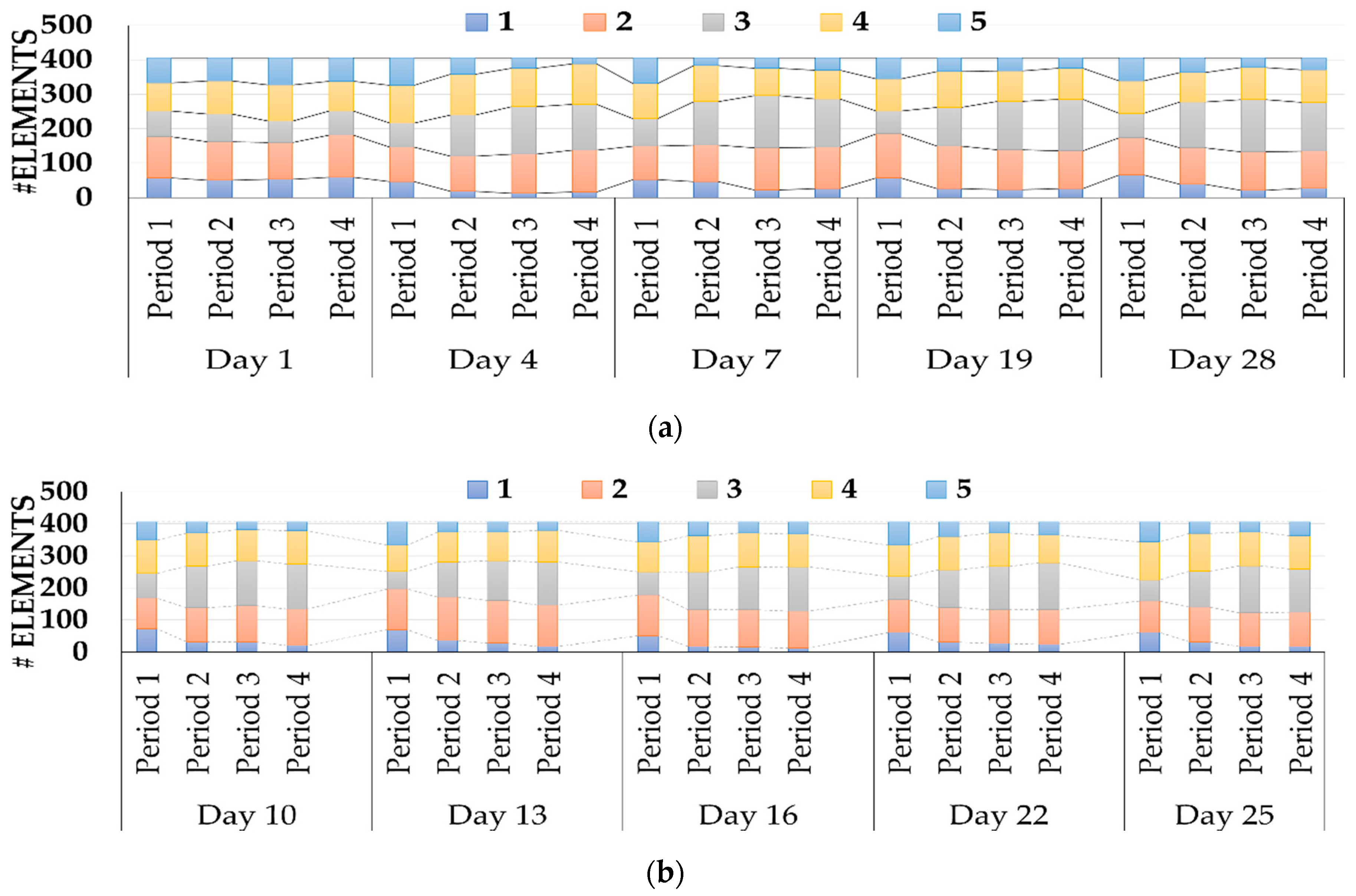
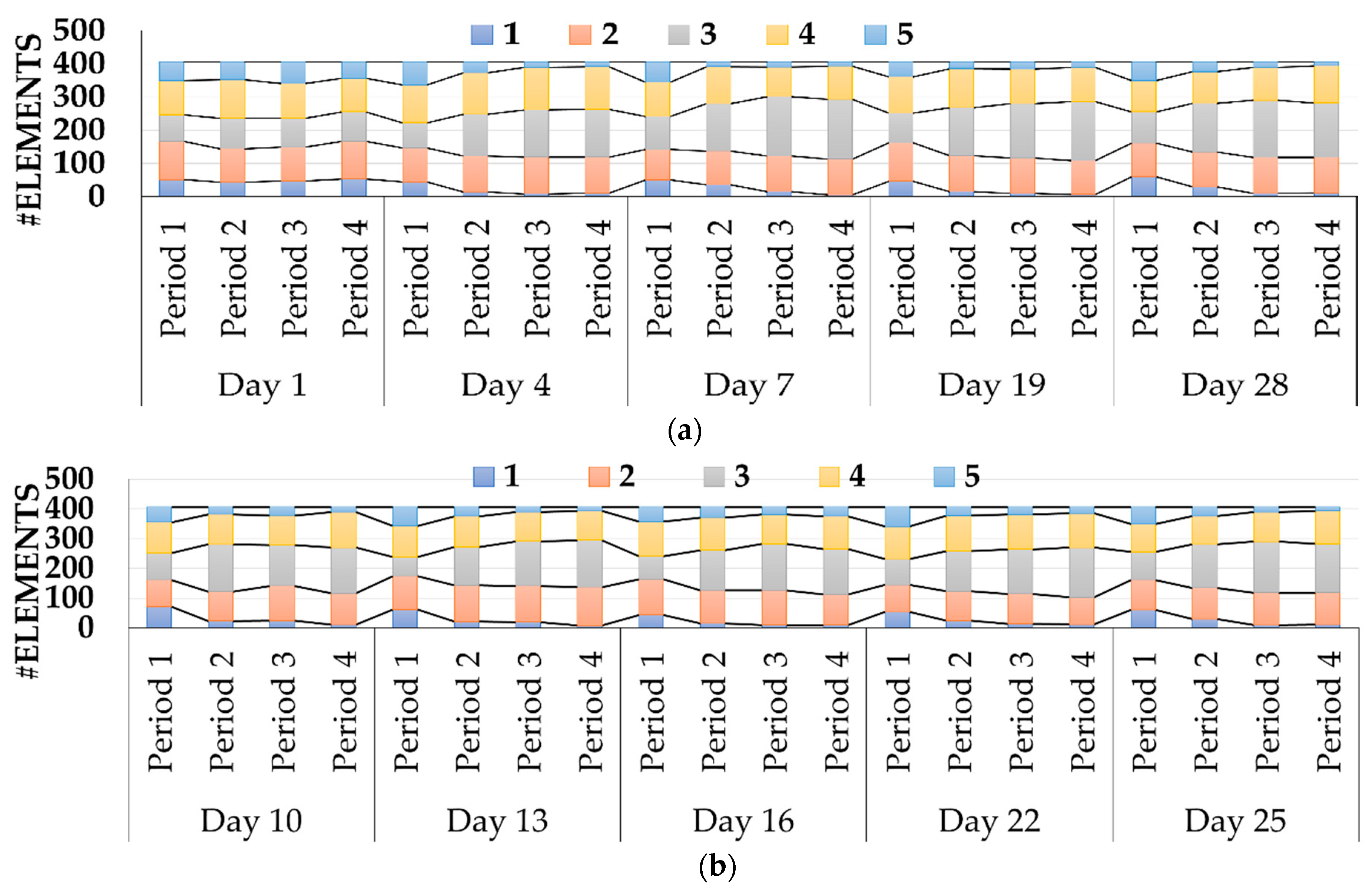
Figure 5 presents the accumulated number of elements in each group per period and day to the two events.

According to the actual response of each consumer, the reliability rate is updated to the final reliability rate of the current period. This rate is considered as LDR for the following day. Additionally with of this value, the Remuneration Rate is found for each Reliability Rate group—regarded as the maximum value detected in each group. When comparing with the results in Figure 3, where the initial number of elements per Reliability Rate was presented, for Event 1, the group with a higher difference was Reliability Rate 3—the number of elements reduced for all the DR event periods when comparing. The second group with the lower number of elements was Reliability Rate 4. For Reliability Rate 1 and Reliability Rate 2, the number of elements floated but always above the initial value. Regarding Reliability Rate 5, the highest difference record achieved an increase of 288.89% from the initial value: Day 28, Period 4—started with nine elements and finished with 35.

Applying the same analysis to the results from Figure 5b, similar conclusions can retreat: Reliability Rate 3 was the one where the frequency of negative percentages (lower number of elements than initial) was higher, followed by Reliability Rate 4. The Reliability Rate 1 and Reliability Rate 2 had increased their number of elements most of the time. The Reliability Rate 5 also had the highest increase—366.67%, on Day 10, Period 4 – started with six elements and finished with 28.

Having the updated rates,

Table 6. Remuneration.

	Day	Period 1		Period 2		Period 3		Period 4		Total Day
		(m.u.)	#	(m.u.)	#	(m.u.)	#	(m.u.)	#
Event 1	1	27.64	73	28.30	71	27.32	70	28.02	68	111.28
	4	28.33	50	28.84	60	25.06	58	25.39	53	107.62
	7	27.19	73	28.02	72	26.86	70	27.87	71	109.94
	19	28.05	75	27.11	71	27.95	70	24.91	68	108.02
	28	27.00	72	25.83	72	26.59	69	27.17	67	106.59
Total Period		138.21	-	138.10	-	133.78	-	133.36	-	543.45
	Day	Period 1		Period 2		Period 3		Period 4		Total Day
		(m.u.)	#	(m.u.)	#	(m.u.)	#	(m.u.)	#
Event 2	10	27.13	61	27.05	60	25.87	70	27.20	73	107.25
	13	26.98	73	26.63	73	25.57	58	23.85	60	103.03
	16	26.88	68	25.26	67	24.54	65	24.30	64	100.98
	22	26.44	70	26.16	69	25.84	72	25.28	82	103.72
	25	25.09	69	25.39	75	24.94	75	25.76	74	101.18
Total Period		132.52	-	130.49	-	126.76	-	126.39	-	516.16

introduces the remuneration values per period, day and event, and the number of consumers’ needs for each period to achieve the DR target (# is the number of elements).

According to the total remuneration per period, Period 4 is the one where the Aggregator spends less in the compensation of the participants in the management of the community, for both events. The total remuneration for Event 1 was higher than Event 2 because, in 14 of this event periods, the value of actual reduction was much higher than the DR event (considering values below 105 kW acceptable).

3.2. Cost Rate Method

The Cost Rate Method is a variant from the Basic Rate Method. The consumers that were not able to increase their Reliability Rate may decrease their DR event cost to be selected by the optimization in the Scheduling phase of the next period for the following DR event. As mentioned, this method and the following will not have the same detailed explanation and analysis of the Basic Rate Method.

3.2.1. Initial Reliability Rate

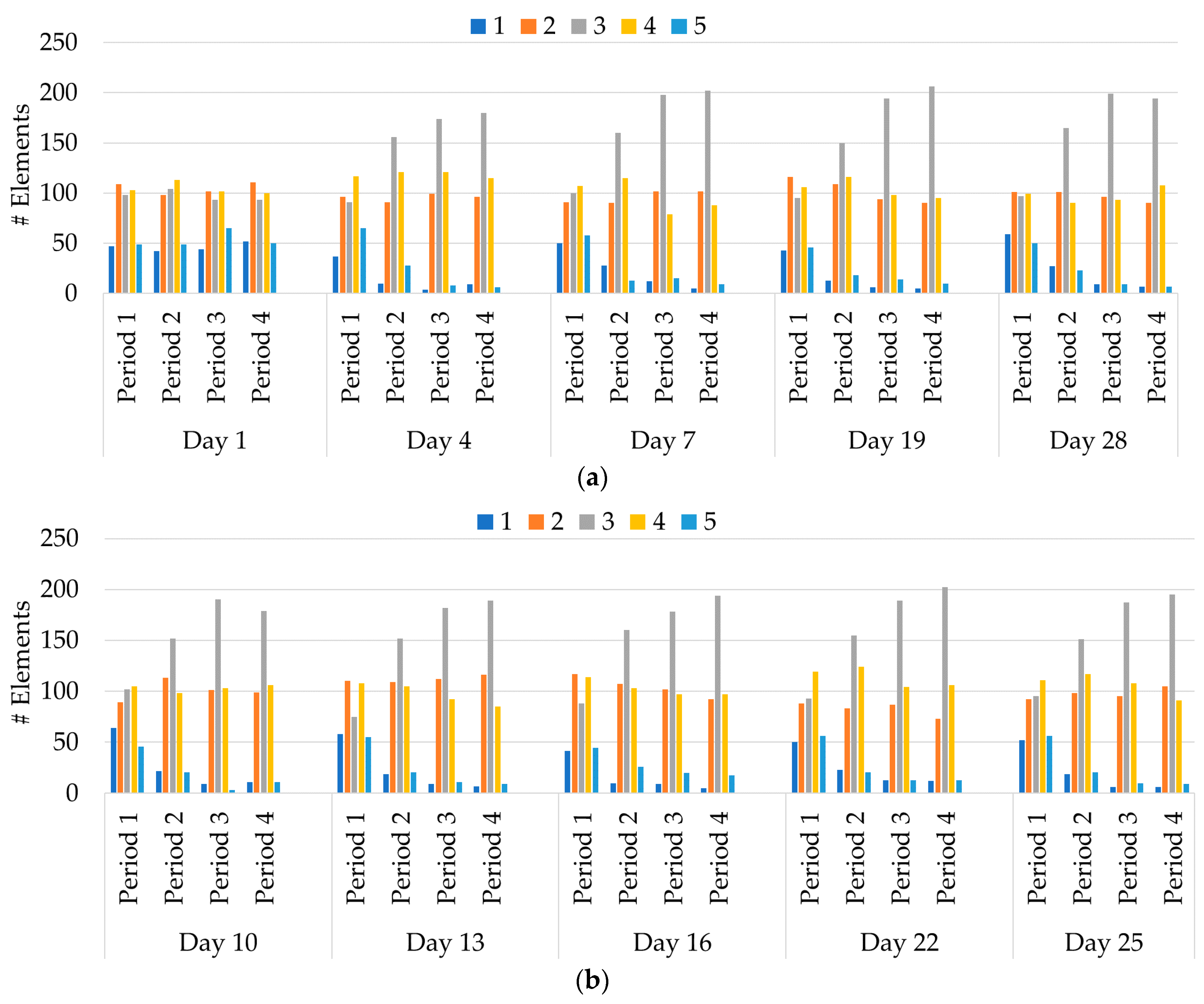
Figure 6 introduces the initial number of elements in a Reliability Rate group per day and period. The assumptions from Basic Rate Method for this phase are now applied: The initial reliability rate considers the HR and the LDR. Moreover, the first day of each event does not have an LDR so, only HR is applied. By analyzing Figure 6a, one of the points that stand out is the reduction of the number of elements from Reliability Rate 5 through the days until it reaches a null value. This fact will have a massive impact on the performance of this method—considering that only the elements with reliability rates above the denominated minimum can join the scheduling phase. If the consumers with Reliability Rate 3 and Reliability Rate 4 do not have enough reduction power available, a Re-scheduling stage will be needed to achieve the DR target. Another highlight is the fact that the number of elements from Reliability Rate 2 highly increased overtime. When comparing the number of elements in the first day of this type of event with the last one, the total of elements able to participate in Period 1 decreased by 1.60%. Regarding Period 2, the number of elements increased by 1.88%. The difference for Period 3 was the highest being −49.62% from the initial value of participants. The amount of Period 4 was also high, being −34.98%.

About Event 2, the reduction of elements for Reliability Rate 5 started right on the first day of the event, unlike Event 1. Giving this, the effect in the comparison between the number of elements in the first day with the last one was not so impactful. From Period 1 to 3, the number of elements floated but always increased. Period 4, instead, decreased by 3.27%.

3.2.2. Scheduling and Re-Scheduling Results

Due to space limitations in this paper, the results are not shown for this method. Anyway, it has been computed, and the rate update and remuneration are given in the next sub-section.

According to Figure 2, when the method that selected the consumers were not able to achieve the DR event in the Scheduling, one or several Re-scheduling must be done. In this case, a maximum of five more iterations was needed to accomplish the DR target. On Day 16 and Day 25, the first two periods were able to meet the goal in the Scheduling. For Day 7, Day 10, Day 13, Day 19, Day 22, only in Period 1 the objective was achieved with a Scheduling. In total, the Re-Scheduling step was needed 31 times.

3.2.3. Rate Update and Remuneration

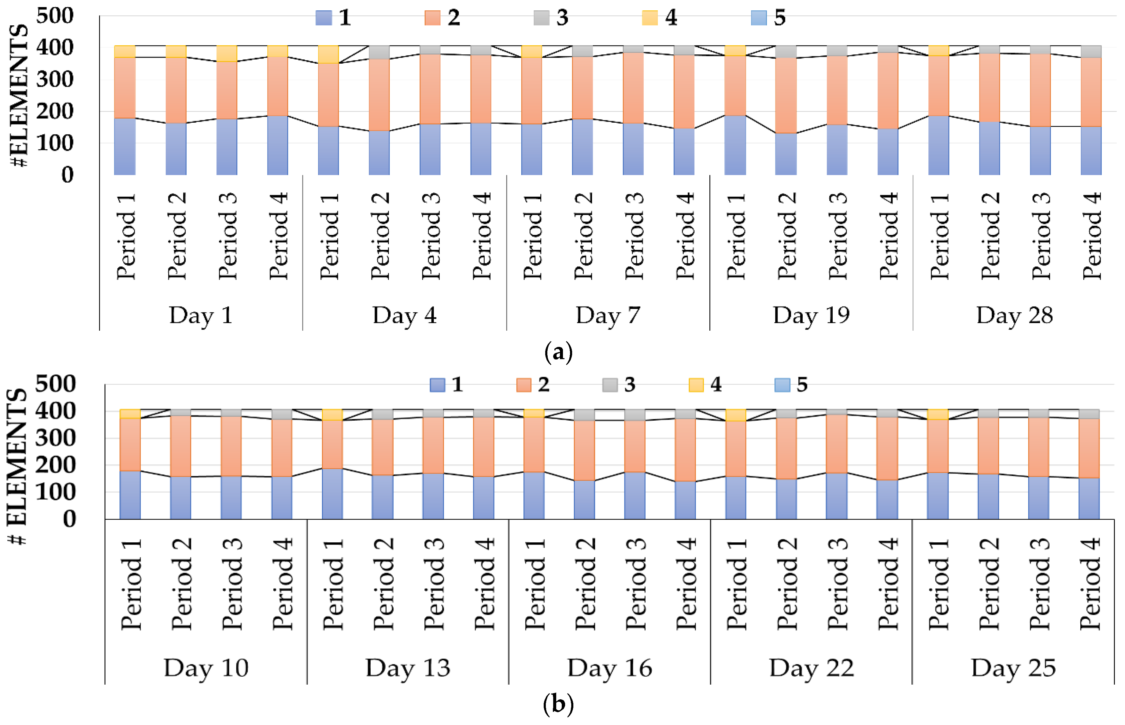
Figure 7 shows the accumulated number of elements for each Reliability Rate group per period, per day, and event. The missing Reliability Rate 5 for both events can be easily noticed.

The formula used to update the reliability rate of each consumer is the same as the Basic Rate Method but, the variant is presented here since the cost from the DR event can be updated according to the reliability rate. In Figure 7a, Reliability Rate 1 was the one with a higher increase of elements when comparing with Figure 6a—starting from +183.33% to +320.93%. Reliability Rate 2 was the other one where this percentage was maintained above 0%. The remaining saw their number of elements reduced. Regarding Figure 7b, the scenario is similar for all days: In the first period, Reliability Rate 4 still had some elements but, over time, tended to null. In this way, the final reliability rate resumed into three groups. The remuneration provided by the Aggregator to the participants and the number of participants per event is in

Table 7. Remuneration.

	Day	Period 1		Period 2		Period 3		Period 4		Total Day
		(m.u.)	#	(m.u.)	#	(m.u.)	#	(m.u.)	#
Event 1	1	27.51	73	28.26	71	28.01	70	26.94	68	110.72
	4	28.00	50	27.03	64	25.55	56	27.95	49	108.53
	7	28.30	73	25.67	33	25.48	53	26.93	41	106.38
	19	27.31	75	26.57	30	26.62	44	28.81	38	109.31
	28	28.31	72	27.98	35	26.05	41	28.33	42	110.67
Total Period		139.43	-	135.51	-	131.71	-	138.96	-	545.61
	Day	Period 1 (m.u.)		Period 2 (m.u.)		Period 3 (m.u.)		Period 4 (m.u.)		Total Day
Event 2	10	25.60	69	25.78	39	25.59	47	25.81	52	102.78
	13	25.85	73	25.04	38	25.82	48	23.96	45	100.67
	16	25.99	68	25.06	52	25.69	48	23.98	59	100.72
	22	24.92	70	23.95	64	24.40	79	25.44	57	98.71
	25	25.58	69	25.87	52	23.96	46	26.56	55	101.97
Total Period		127.94	-	125.7	-	125.46	-	125.75	-	504.85

. The period with a lower value was Period 3 for both events.

Regarding the total remuneration per day, the lower value in Event 1 was on Day 7 with 106.38 m.u. and for Event 2 was Day 22 with 98.71 m.u. When comparing Table 7 with Table 6, along with results from the remuneration of the Basic Rate Method, the number of elements needed to achieve the DR target is generally less.

3.3. Clustering Method

The Clustering Method is another variant from the Basic Rate Method. On the contrary to the Cost Rate Method, the final cost stays the same. The only difference is the technique for participant selection—a clustering method is used to split each reliability rate into groups. The one with the higher accumulated reduction from each reliability rate is selected, and all the elements are selected.

3.3.1. Initial Reliability Rate

The logic for the Initial Reliability Rate calculation is the same as previous methods, only the selection of the consumers to participate in DR events is different. In this way, the HR and the LDR are considered except on the first day of each event. Figure 8 introduces the number of elements per Reliability Rate, for each day and per period. It is also separated by type of event. The number of elements that could participate in the management of the community in the first event of type 1, for Period 1 was 250 being reduced by 1.60% by the last day. In Period 2, a little increase was noticed (1.88%) being the Reliability Rate 3 the group with more elements. For Period 3 and Period 4, the number of elements able to be selected increased by 15.77% and 27.16%, respectively.

Forward to Event 2 results in Figure 8b, Period 1 had an increase of 3.56% in the number of elements above the denominated minimum. For Period 2, the number of elements increase was the same as Event 1. Period 3 had the higher growth of elements in this event and to this comparison being 3.041%. Period 4 was the only one with a reduction, where the number of elements able to participate reduced by 0.03%.

3.3.2. Scheduling and Re-Scheduling Results

The clustering method was applied to each Reliability Rate group above three, and the selected consumers were able to participate in the Scheduling. The days where a Re-scheduling was needed for only one period in the DR event were Day 1, Day 10, and Day 13. Day 4 and Day 16 were the only days where the DR target was achieved with Scheduling in one period, and the remaining needed another iteration. On Day 7, Period 1 and Period 5 went to Re-scheduling. On Day 19 and Day 25, Period 1 and Period 2 went to Re-scheduling. On Day 22, Period 2 and Period 3 went to Re-scheduling. In total, the Re-scheduling step was needed 18 times, the lowest value from the three methods.

3.3.3. Rate Update and Remuneration

With the results from the Scheduling phase, it is possible to revise the Reliability Rate. The Clustering Method has the same formula and weights as the Basic Rate Method, and no DR event costs are changed. In this way, Figure 9 shows the results from this update. Reliability Rate 3 was the one that suffered more changes negatively, since, in all periods of Event 1, the number of elements reduced when compared with the initial value. Reliability Rate 5 was the one with a higher sum of elements when compared with the initial number; however, the maximum number of elements was never higher than 70, as well as Reliability Rate 1. In this way, most elements are concentrated between Reliability Rate 2 and Reliability Rate 4. Regarding Event 2, the picture is similar: Reliability Rate 1 and Reliability Rate 5 with fewer elements, having the last one the higher increase in Day 10, Period 3 passing from 3 to 28 elements. Over periods, regarding Reliability Rate 5, the tendency seems to increase the percentage of elements.

Forwarding to the remuneration of the participants,

Table 8. Remuneration.

	Day	Period 1		Period 2		Period 3		Period 4		Total Day
		(m.u.)	#	(m.u.)	#	(m.u.)	#	(m.u.)	#
Event 1	1	27.85	52	32.60	23	29.57	15	25.61	28	115.63
	4	31.16	28	28.00	28	26.27	25	27.29	22	112.72
	7	32.67	9	29.24	19	29.79	15	25.99	11	117.69
	19	30.93	9	29.21	9	25.67	31	26.98	24	112.79
	28	26.07	12	26.79	24	24.50	20	28.82	22	106.18
Total Period		148.68		145.84		135.80		134.69	-	565.01
Event 2	10	28.28	20	25.58	22	25.68	74	25.63	14	105.17
	13	24.03	31	24.03	32	24.06	28	25.53	17	97.65
	16	24.25	30	28.67	33	25.40	32	25.82	39	104.14
	22	24.93	34	24.02	30	24.75	43	24.59	17	98.29
	25	24.07	35	24.02	31	27.44	27	23.99	26	99.52
Total Period		125.56	-	126.32	-	127.33	-	125.56	-	504.77

presents the compensation values and the number of elements needed to achieve the DR event target. For the analysis of Event 1, the most expensive period was the first one. Still, over time the value reduced being the last one the cheapest from the perspective of the Aggregator—also, fewer members were needed to achieve the target.

In Event 2, the final remuneration per period was around 125 m.u., the lowest value achieved in both Period 1 and Period 4. This event was also the cheapest to the Aggregator (in days: 504.77 m.u.).

3.4. Consumer Reliability Rate Identification for Month—k-Means

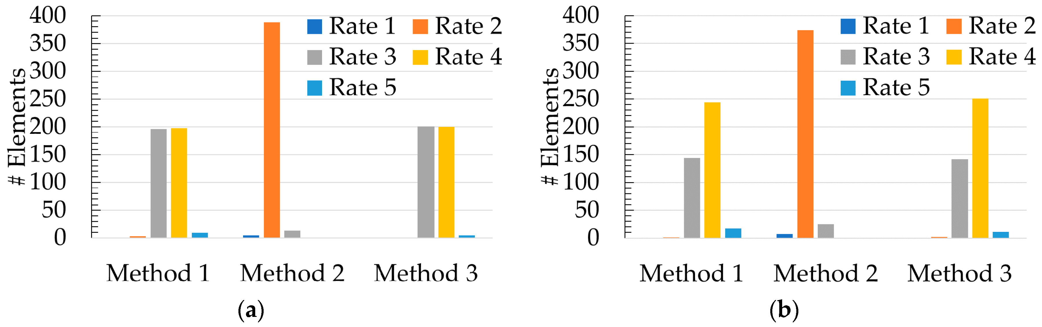
A clustering method was used to identify a Month Reliability Rate to each consumer. This approach was already applied for Clustering Rate Method. The idea is to study the centroid value to assign proper rates according to the performance of that consumer over the entire month, for both events. In this way, per consumer, a monthly curve per event was designed, and the rate was designated with the maximum value found in the mentioned curve.

Figure 10 presents the total elements per Reliability Rate. The three methods were compared, and the groups with null values were hidden. Considering that the Basic Rate Method is Method 1, Cost Rate Method is Method 2, and the Clustering Rate Method is Method 3. Starting with Method 1, Figure 10a finds the more significant number of elements between Reliability Rate 3 and Reliability Rate 4 with a total of 394 elements. The other 12 elements were attributed to Reliability Rate 2 and Reliability Rate 5.

The results from Figure 10b are similar, although Reliability Rate 4 has more elements this time: 244 elements. Moreover, Reliability Rate 4 increased the number of elements. Method 2 has the highest number of elements in Reliability Rate 2 for both events: Event 1 with 388 and Event 2 with 374. The remaining consumers were attributed to Reliability Rate 1 and Reliability Rate 3. Finally, Method 3 results were similar to Method 1. In Figure 10a, most consumers are centered between Reliability Rate 3 and Reliability Rate 4, where the remaining were assigned to the higher reliability rate. Regarding Figure 10b, Reliability Rate 4 has 251 elements when comparing with the 142 of Reliability Rate 3. The missing 13 were assigned to Reliability Rate 2 and Reliability Rate 5. To justify these results and understand the behaviour of some consumers the following

Table 9. Final Reliability Rate from selected consumers when using Method 1.

Consumer ID	Final Month Rate		Reliability Rate 1	Reliability Rate 2	Reliability Rate 3	Reliability Rate 4	Reliability Rate 5
	Event 1	Event 2
41	4.40 (4)	4.00 (4)	8	12	2	3	15
119	3.20 (3)	3.00 (3)	0	12	18	10	0
162	4.00 (4)	4.00 (4)	1	6	17	13	3
232	3.00 (3)	4.20 (4)	7	14	6	6	7
356	3.40 (3)	3.00 (3)	6	9	14	11	0

,

Table 10. Final Reliability Rate from selected consumers when using Method 2.

Consumer ID	Final Month Rate		Reliability Rate 1	Reliability Rate 2	Reliability Rate 3	Reliability Rate 4	Reliability Rate 5
	Event 1	Event 2
41	1.80 (2)	2.00 (2)	16	24	0	0	0
119	2.00 (2)	1.80 (2)	16	20	4	0	0
162	2.00 (2)	2.40 (2)	11	25	2	2	0
232	1.60 (2)	2.00 (2)	23	16	0	1	0
356	2.20 (2)	2.00 (2)	16	19	5	0	0

and

Table 11. Final Reliability Rate from selected consumers when using Method 3.

Consumer ID	Final Month Rate		Reliability Rate 1	Reliability Rate 2	Reliability Rate 3	Reliability Rate 4	Reliability Rate 5
	Event 1	Event 2
41	4.00 (4)	4.40 (4)	3	9	8	12	8
119	3.20 (3)	3.00 (3)	1	12	17	10	0
162	4.00 (4)	4.00 (4)	1	6	17	13	3
232	2.80 (3)	3.60 (4)	7	17	8	5	3
356	3.40 (3)	3.00 (3)	6	9	14	11	0

present the results from five selected consumers for Method 1, Method 2, and Method 3, respectively.

Consumer 41 and Consumer 162 were assigned to Reliability Rate 4 for both events in Method 1 and Method 3. In Method 2, both decreased two levels. Consumer 119 and Consumer 356 were assigned by Method 1 and Method 3 to Reliability Rate 3 and by Method 2 to Reliability Rate 2. Consumer 232, in Method 1, was assigned to Reliability Rate 3 in Event 1 and Reliability Rate 4 in Event 2. In Method 2, the Reliability Rate 2 was attributed to this consumer. Finally, Method 3 was assigned the Reliability Rate 3 in both events.

3.5. Reliability Rates over Different Seasons

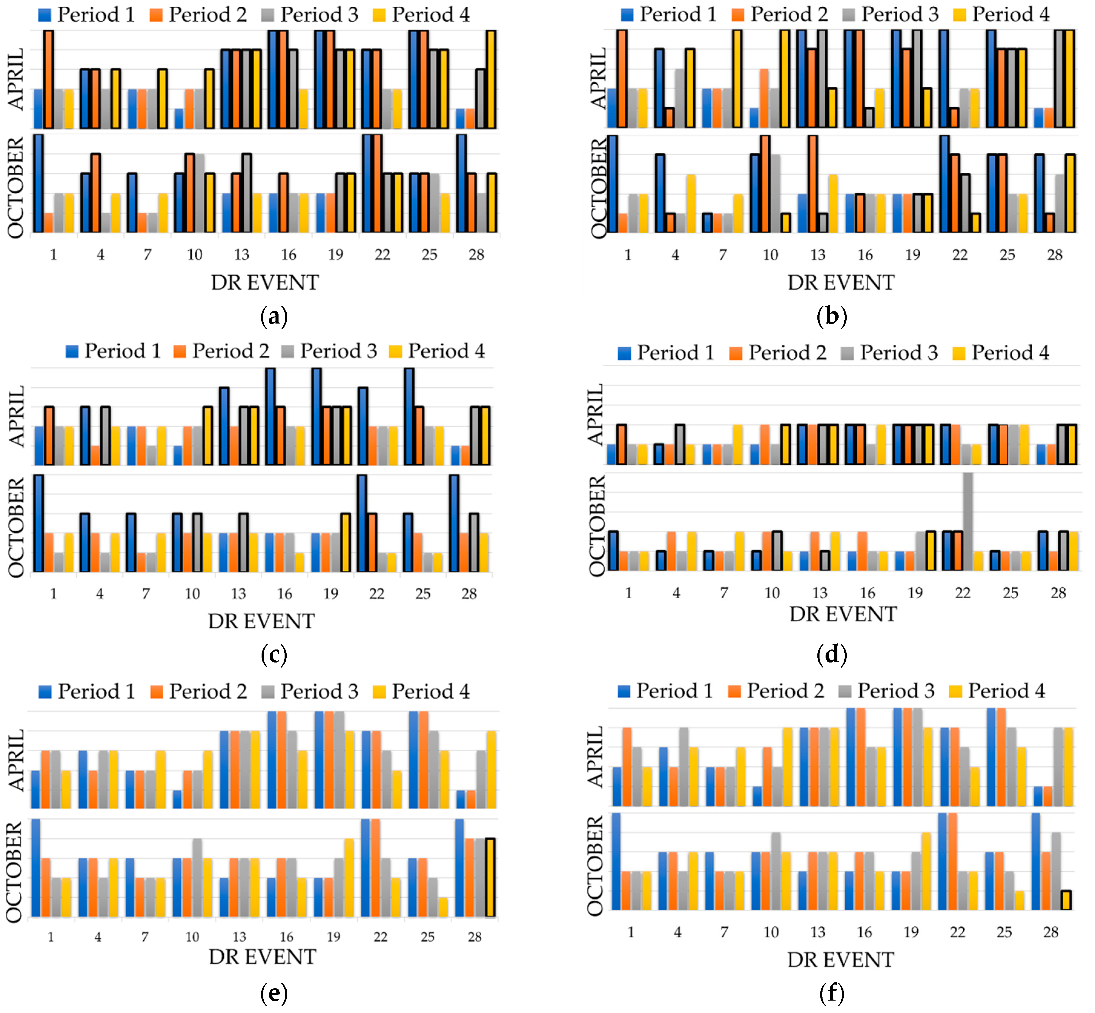
From the previous sub-sections, one consumer was chosen by the authors to examine the behaviour and the possibility of reliability change throughout the year. In this way, prior results from April were compared with a month in another season with October in Autumn being chosen. October 2018, in Portugal, was classified as usual regarding air temperature and as dry concerning precipitation. The month of April 2018 was pouring and normal regarding air temperature.

Figure 11 presents both initial and final rates for Consumer 41 to the ten different events simulated in these months. The highlight rates (black outline) represent the times when the consumer was selected to participate in the scheduling. Method 1, for both months, was the one that considered more times in the management of the local community.

On the contrary, Method 3 only chooses this costumer one time. Using a clustering approach where only the ones with the higher value of reduction are adopted, it can be concluded that a re-scheduling was needed in the DR event from October 28, also considering the consumers with Reliability Rate 4. In this way, the detailed overview of Method 1 and Method 2 was done. Regarding the comparison between the initial and final rate for both months, studying the availability and the possibility of reliability change through seasons, for Method 1, for the selected consumer the results were inferior in October since there was a decrease in the reliability rate 30% across the several DR events comparing with 18% from April. The highest share is represented by the equal reliability rate: 45% in October and 55% in April and the periods where the reliability rate increased represent 25% and 28% for October and April, respectively. However, the actual response from this consumer did not have a considerable difference between the selected months and seasons. The authors of the present paper consider that further studies must be done regarding the number of days submitted to DR programs, differences between periods of the day and compensation. Regarding Method 2, the values were worst in April since 70% of the reliability rates decrease over the DR events.

The authors are aware that this study did not represent all communities but goes according to what was said by Srivastava et al. [27] in their research understanding the willingness of the consumers to accept limits on the use of smart appliance-based DR program in return for a recompense. One of the main conclusions from these authors was that consumers are motivated by the amount of compensation they would receive for the flexibility given. Since one of the main focuses of the small consumers is the comfort—the abdication of this goal would require high remuneration. Therefore, this method must be reformulated.

4. Conclusions

The solution proposed in the present paper has as the main goal of defining a proper approach to aid the Aggregator in the complex management of small resources in a local community, taking into account the uncertainty associated with the demand response. The literature presents fewer approaches considering this problem. Hence, the authors introduce, as a noble factor from previous works, a Reliability Rate that will be useful to decide which consumers this entity may trust in a certain period for a DR event with a specific DR target. The goal is to minimize the operation costs, for the Aggregator, with an optimization to manage all the resources associated with this entity— small consumers and DG are considered, and still achieve the DR target when DR events occur. The case study had a dataset with information from all the resources for a whole month. Regarding the Scheduling phase, the proposed methodology is suitable to be used as a tool to aid the Aggregator in the management of a local community where DR targets are applied. Although some periods need Re-scheduling, it is considered as a successful approach to deal against the uncertainty of the consumers and a step forward when comparing with previous works by the authors since the DR target was always achieved. The technique of aggregate consumers with higher reduction power between the rates with more reliability was the one with lower failures. Additionally, from the perspective of the Aggregator, the one with lower remuneration costs.

By analyzing results from three methods, the duration of the DR event as an impact on the actual response of the consumers. Independent of the event, when comparing the first period and the remaining, a notorious increase of Reliability Rate 3 can be noticed. Several conclusions can be withdrawn from this study:

• A 15-min interval between actualizations of the actual response is a bearable time for a DR event to have more reliable answers and understand the condition of each consumer;
• The Aggregator, as a community manager, must take into account not only the past information but also the actual response for the previous event in the calculation of the initial rate to consider the results of earlier events. Although the historic quota is relevant, the behaviour of the consumer and recent information may indicate a change useful for the reliability;
• The remuneration for participating in DR programs is essential. When the value of compensation decreases, the consumers were less willing to contribute to the balance of the local community.

Overall, the approach implemented in this paper is found to be useful in assessing and rewarding the consumers’ performance, giving reliability signals to the Aggregator after the enrolment phase, in opposition to traditional approaches where consumer participation in DR is assessed in each event individually.

Anyway, more improvements and further studies are needed. As future work, authors intend to investigate: The behaviour of consumer—according to the period of the day, day of the week, and month or even to an entire season. The ways to incentivize their participation is to increase their reliability rate since the consumption habits can vary through the year and the right remuneration is crucial.