Article

sDeepFM: Multi-Scale Stacking Feature Interactions for Click-Through Rate Prediction

1
Guangxi Cloud Computing and Big Data Collaborative Innovation Center, Guilin 541004, China
2
Guangxi Key Laboratory of Image Graphics and Intelligent Processing, Guilin University of Electronic Technology, Guilin 541004, China
*
Author to whom correspondence should be addressed.
Electronics 2020, 9(2), 350; https://doi.org/10.3390/electronics9020350
Submission received: 20 January 2020 / Revised: 13 February 2020 / Accepted: 17 February 2020 / Published: 19 February 2020
(This article belongs to the Special Issue Regularization Techniques for Machine Learning and Their Applications)

Abstract

:
For estimating the click-through rate of advertisements, there are some problems in that the features cannot be automatically constructed, or the features built are relatively simple, or the high-order combination features are difficult to learn under sparse data. To solve these problems, we propose a novel structure multi-scale stacking pooling (MSSP) to construct multi-scale features based on different receptive fields. The structure stacks multi-scale features bi-directionally from the angles of depth and width by constructing multiple observers with different angles and different fields of view, ensuring the diversity of extracted features. Furthermore, by learning the parameters through factorization, the structure can ensure high-order features being effectively learned in sparse data. We further combine the MSSP with the classical deep neural network (DNN) to form a unified model named sDeepFM. Experimental results on two real-world datasets show that the sDeepFM outperforms state-of-the-art models with respect to area under the curve (AUC) and log loss.

1. Introduction

The click-through rate (CTR) prediction task is to estimate the probability of a user’s clicks on certain delivered ads for a given user, commodity, and interactive behavior, and to measure the popularity of the ads. Therefore, accurate click-through rate estimation can reduce the invalid delivery of ads, which is directly related to the revenue and user experience of the advertising platform. Various systems were developed by different companies [1,2,3]. As the most critical part of online advertising, advertising click rate estimation has very important theoretical research and practical value.
Professor Domingos at Washington University pointed out that the features used are a key factor in the success of many machine learning projects [4]. The classification of things by human beings is mainly based on the common characteristics and differences between things. Similarly, the classifier relies on descriptive information that can make contact and distinguish between things. This information represents the features of things. However, it is still a very challenging task in constructing features to provide an accurate click-through rate estimation for ads, which is subject to several aspects. Firstly, it is too costly to construct features manually. Feature generation is the process of portraying things from different angles and sides. However, the feature dimensions of advertising data are usually extremely high, and it is almost impossible to hand-craft all the meaningful combinations [5]. Therefore, a structure that can automatically construct the feature combinations is a core issue that needs to be addressed in current click-through rate estimation tasks. Secondly, the traditional models that automatically construct feature interactions focus mainly on low-order features or higher-order features, and the features built are relatively simple. How to mine features with different scales from multiple angles to ensure the diversity of information learned by the model is a key issue. Thirdly, advertising data are extremely sparse and high-dimensional [6]. When learning the parameters of k-order features, few samples satisfy the requirement that all the k features of a sample are not 0, leading to difficulty in learning k-order features. Thus, how to learn the higher-order features in the extremely sparse data is also a key issue.
For example, logistic regression (LR), as the most classic classifier, has the advantages of simple form, good interpretability of the model, and fast training speed. However, it cannot construct features automatically and relies too much on artificially constructed features. Degree-2 Polynomial Margin (POLY2) [7] can learn the second-order combination features. However, if the combination of a feature does not appear in the training set, the weights of corresponding terms cannot be fully learned, thus reducing the accuracy of prediction. In particular, when dealing with the data using the method of one-hot to process the features, the eigenvector becomes extremely sparse. The data become sparser after POLY2 crosses the features, leading to the inability for most weights of the cross features to be learned because of a lack of effective data. Factorization machines (FM) [8] express features through hidden vectors such that the weights of second-order combined features can be decomposed into the product of two implicit vectors. However, since the calculation of the higher-order features cannot be simplified, the time complexity is very high. In general, FM only considers the first- and second-order features, which is also a limitation of FM. The field-aware factorization machine (FFM) [9] introduces the concept of a field based on the FM model and proposes a factorization machine oriented to the feature fields. Each feature will learn different implicit vectors according to different feature fields, which makes the learning more elaborate. However, it also brings the problem that the model is too complex and the time complexity is too high. With the improvement of computation force and the breakthrough of theory, neural networks are becoming increasingly popular in the machine learning field [10]. Deep learning technology with autonomous learning ability was widely researched and made surprising progress in feature learning [11]. Especially in the click-through rate prediction system, the deep learning method basically replaced the traditional machine learning models in academia and industry. The Wide&Deep [12] proposed by Google is an early influential CTR prediction scheme based on a deep learning model. This model jointly trains the wide part which is a single-layer neural network and the deep part which is a multi-layer deep neural network. The wide part pays more attention to the memory, while the deep part pays more attention to the generalization and inference. However, the Wide&Deep relies too much on artificially constructed features. The factorization machine deep neural network (FNN) [13] obtains a dense embedding vector of each feature through pre-training an FM model and combines all embedding vectors as the input of a deep neural network (DNN). The advantage is that it uses the intermediate product from the embedding vector of FM to reduce the features, and the deep neural network can not only perform the nonlinear changes of higher order, but also has the function of feature extraction. The disadvantage is that, considering the time complexity, the factorization machine can only extract combinations of the second-order features, and the deep neural network is complex and difficult to train and converge. The product-based neural network (PNN) [14] changes the structure of Wide&Deep by adding crossed features to the input of the neural network. The pairwise cross-calculation of eigenvectors can be seen as FM, which can construct features artificially. The attentional factorization machine (AFM) [15] filters the meaningless features through the attention mechanism, solving the problem that the middle layer may produce useless features and even increase the noise, which can interfere with the model on the feature combination. However, the limitation of PNN and AFM is that only low-order features are considered. DeepFM [16] divides the embedding vector into two parts. One part is the input of FM, while the other is the input of a deep neural network. DeepFM considers the low-order features and higher-order features, but the output is only combined as FM and DNN. We want a new way of constructing features, which can achieve higher accuracy. xDeepFM [17] is one of the most advanced models that integrates the Compressed Interaction Network (CIN) and DNN modules, which can help the model to learn high-order feature in both explicit and implicit ways, while the integrated linear module and deep neural module also enable the model to have both memory and generalization ability. However, the model is too complex and the executing time of the model is too long.
In order to solve these problems, we designed a new feature extraction structure called multi-scale stacking pooling (MSSP). The core idea is to construct multiple observers with different angles and horizons to explore the features from multiple angles and scales in multi-scale space. Each detector learns parameters by factor decomposition to solve the problem that it is difficult to learn higher-order features in sparse data. Our model outperforms the state-of-the-art models on two public datasets. The primary contributions of the proposed model sDeepFM can be summarized as follows:
  • A novel structure named multi-scale stacking pooling based on different receptive fields for multi-scale feature extraction is proposed, which mines high-order and low-order features in different local information from the directions of depth and width to ensure the diversity of extraction features.
  • By learning parameters using factorization, the parameters of cross-terms are no longer independent of each other. With more hidden vectors of higher-order features, the model has more samples to learn, which largely alleviates the difficulty of learning higher-order features in sparse data.

2. Methods

2.1. Problem Description

For the dataset containing n instances and m views, D = { ( x i , y i ) | i = 1 , , n } , in which X T = ( x ( 1 ) T , , x ( m ) T ) and y i { 0 , 1 } is the label of the i-th instance. For the click-through rate problem, 0 represents no click, and 1 represents click. Our task is to learn a function f : R I 1 × × R Im { 0 , 1 } . If y i R , it is a regression problem.

2.2. Model Description

As shown in Figure 1, the proposed sDeepFM model includes three modules, namely, a data input processing module, an automatic feature interaction module, and an output processing module. The input module is mainly used to receive and preprocess the original data. The function of the automatic feature interaction module is to generate diverse features. The module consists of two parts: multi-scale stacking pooling (MSSP) and a DNN. MSSP mines the high-order and low-order features in different local fields of view from the depth and width angles to ensure the diversity of the extracted features; DNN is dedicated to exploring high-order implicit information between features. The output processing module maps the two parts of features to the same dimension and inputs them into the last prediction layer after fusion. Finally, the prediction result is the predicted click-through rate of an advertisement.

2.2.1. The Input Processing Module

In the task of predicting the click-through rate for display ads, the features used usually include classification features, such as the genders of users and the city they are in. Classification features cannot be directly used for calculation, and usually require one-hot encoding preprocessing. If classification feature C has M possible values in the dataset, C is encoded into an m-dimensional vector composed of binary elements. The one-hot encoding is shown in Equation (1).
C = ( b 1 , b 2 , , b M ) ,
where i = 1 M b i = 1 , and b i { 0 , 1 } . In the DNN, nodes of the input layer are fully connected with the hidden layer. Using the original encoded feature vectors directly as the input of the hidden layer will lead to huge computational overhead. Therefore, we propose adding an embedding layer between the input layer and the first hidden layer to reduce the number of input units of DNN. Firstly, each one-hot encoded vector is mapped into a fixed-dimensional embedded vector, and then all the embedded vectors which an instance contains corresponding to the features are spliced together as the input. The initial values of the embedded vectors are set randomly, and the mappings of the embedded vectors are jointly trained as a part of the model; then, the weights are obtained through learning.

2.2.2. The Automatic Feature Interaction Module

The automatic feature interaction module is the core of the model, which consists of three parts. The first part is the proposed method of constructing features: multi-scale stacking pooling (MSSP). MSSP bidirectionally stacks multi-scale features from depth and width, which is responsible for mining high-order and low-order features in different local views. The second part is the DNN module, which is responsible for exploring high-order implicit information between features.
  • Multi-scale stacking pooling
For predicting click-through rates of display advertising, it is of great significance to observe data from multiple perspectives to construct rich features. Similar to humans observing objects, if the detected angles are different, the states observed tend to be different. Furthermore, if the receptive fields are different, the details captured are different. Drawing on this idea, we construct multiple observers which observe from different angles and receptive fields. For example, some observers observe the interaction behavior of user, some observe the attributes of commodity, and some observe the information of shops. At the same time, the receptive fields observed by these observers are also different. Some observers have large receptive fields, and the scale of the constructed features is relatively rough, which can capture the global information of the data, corresponding to the high-order features; some observers have small receptive fields, and the scale of the constructed features is relatively fine, which can capture more details, corresponding to the low-order features. Through these observers with different angles and different fields of view, we can mine features in multi-scale space and ensure the diversity of information learned by the model. This is the newly proposed feature extraction method called multi-scale stacking pooling (MSSP), which is defined as
MSSP = [ MVP 1 ( 1 ) , , MVP w ( d ) ]   ( d 1 , 2 , 3 , , m ,     w Z * ) ,
where MVP ( d ) denotes the observers described above, m is the highest order of the features, and d represents the depth of observation, that is, the size of the receptive field. A larger d denotes a deeper observation and a larger receptive field. In this way, the model captures the global information and constructs the higher-order features. On the contrary, a smaller d denotes a lighter observation and smaller receptive field. In this way, more detailed information is featured, and the model constructs the lower-order features. Each MVP ( d ) observes the feature set { f 1 , f 2 , , f d } . Different feature sets mean different observation angles. Additionally, w represents the number of MVP ( d ) , which is the width of the horizontal stack lever of the model. Of course, a wider model is not better, as an excessively wide model will lead to over fitting. We discuss the two parameters w and d in our experiments.
For each MVP ( d ) , the full-order interactive features from the first order to the highest order in the feature set { f 1 , f 2 , , f d } are learned, and the model is expressed as in Equation (3).
MVP ( d ) = i 1 = 1 I 1 + 1 i m = 1 I m + 1 w i 1 i m ( p = 1 m z i p ( p ) ) ,
where z i p ( p ) = { 1   i p = I p + 1 x i p ( p )   otherwise   .
The number of parameters in Equation (3) is p = 1 m ( I p + 1 ) , which is too huge to learn. Inspired by the FM method of reducing the number of parameters through low-rank decomposition, we reduce the number of parameters through CP decomposition, and we can decompose the calculation of the weight solution as follows:
w i 1 i m = f = 1 k p = 1 m a i p , f ( p ) ,
where K is the size of the embedded vector. We substitute Equation (4) in Equation (3) to obtain a simplified expression.
y = i = 1 I 1 + 1 i m = 1 I m + 1 w i 1 i m ( p = 1 m z i p ( p ) )     = f = 1 k ( i 1 = 1 I 1 z i 1 ( 1 ) a i p , f ( 1 ) + a I 1 + 1 , f ( 1 ) ) ( i m = 1 I m z i m ( m ) a i m , f ( m ) + a I m + 1 , f ( m ) ) .
After simplifying the expression with CP decomposition, the number of parameters reduces to k f = 1 m ( I p + 1 ) = k × n + k × m = O ( k ( n + m ) ) , in which, m << n. The time complexity is the number of parameters of one MVP ( d ) . According to Equation (2), MSSP consists of w MVP ( d ) ; thus, the time complexity and parameter complexity of MSSP is O ( wk ( n + m ) ) , in which m << n. The complexity of the model is linear, which can ensure the model is applicable for online advertising recommendation tasks. Meanwhile, parameter factorization makes the parameters of the cross terms independent of each other, ensuring that high-order features can be effectively learned in sparse data.
  • DNN component
In terms of the ability to express complex functions, a neural network with a shallow structure has certain limitations and cannot represent high-dimensional complex functions, but a deep neural network can be very expressive. Therefore, it is meaningful to introduce a deep neural network to research feature expression for big data mining and predictive analysis of CTR. We use a feed-forward neural network containing multiple hidden layers to learn the high-order interaction information between features, where the embedded layer is fully connected with the first hidden layer. The output of the first hidden layer is calculated by
h 1 = f ( W 0 h 0 + b 0 ) ,
where h 1 is the output vector of the first hidden layer, W 0 is the weight of the embedded layer to the first hidden layer, and b 0 is the bias of the first hidden layer. Both the number of nodes in each hidden layer and the number of the hidden layers can be adjusted. Each node between the hidden layers is fully connected, and the output of the l + 1 -th hidden layer is calculated according to Equation (7), where W l is the weight between the l -th hidden layer and the l + 1 -th hidden layer, h l is the output of the l -th hidden layer, and b l is the bias of the   l + 1 -th hidden layer.
h l + 1 = f ( W l h l + b l ) .

2.2.3. The Output Processing Module

The function of the output processing module is to fuse the features from three parts of the automatic feature interaction module for the last prediction layer. To prevent the feature dimension differences from affecting the contribution of the three modules to the model, we map the three-part features to the same dimension, and then merge them as the input of the final prediction layer. The input vector is expressed as
h L = [ y MSSP , y D N N ] .
The last prediction layer is expressed as
h p = sigmoid ( W L h L + b L ) ,
where W L is the weight of the feature mapping layer to the prediction layer, h L is the output of the mapping layer, and b L is the bias of the prediction layer. The sigmoid function is employed as the activation function to calculate the predicted click-through rates.

2.3. Model Learning

In this section, we introduce the learning of the model. Firstly, the loss function is introduced, then the training process of the model is introduced, and finally how to predict the click-through rate of advertisements through our model is introduced.

2.3.1. The Loss Function

Our loss function is log loss, which is defined as follows:
L ( h p , y ) = log ( 1 + exp ( y h p ) ) ,
where hp is the result calculated by Equation (9), i.e., the probability of a user’s click on an advertisement, and y is the actual label. Through the loss function, we can calculate the error between the predicted value and the real value, which provides the benchmark for model learning.

2.3.2. Training Process

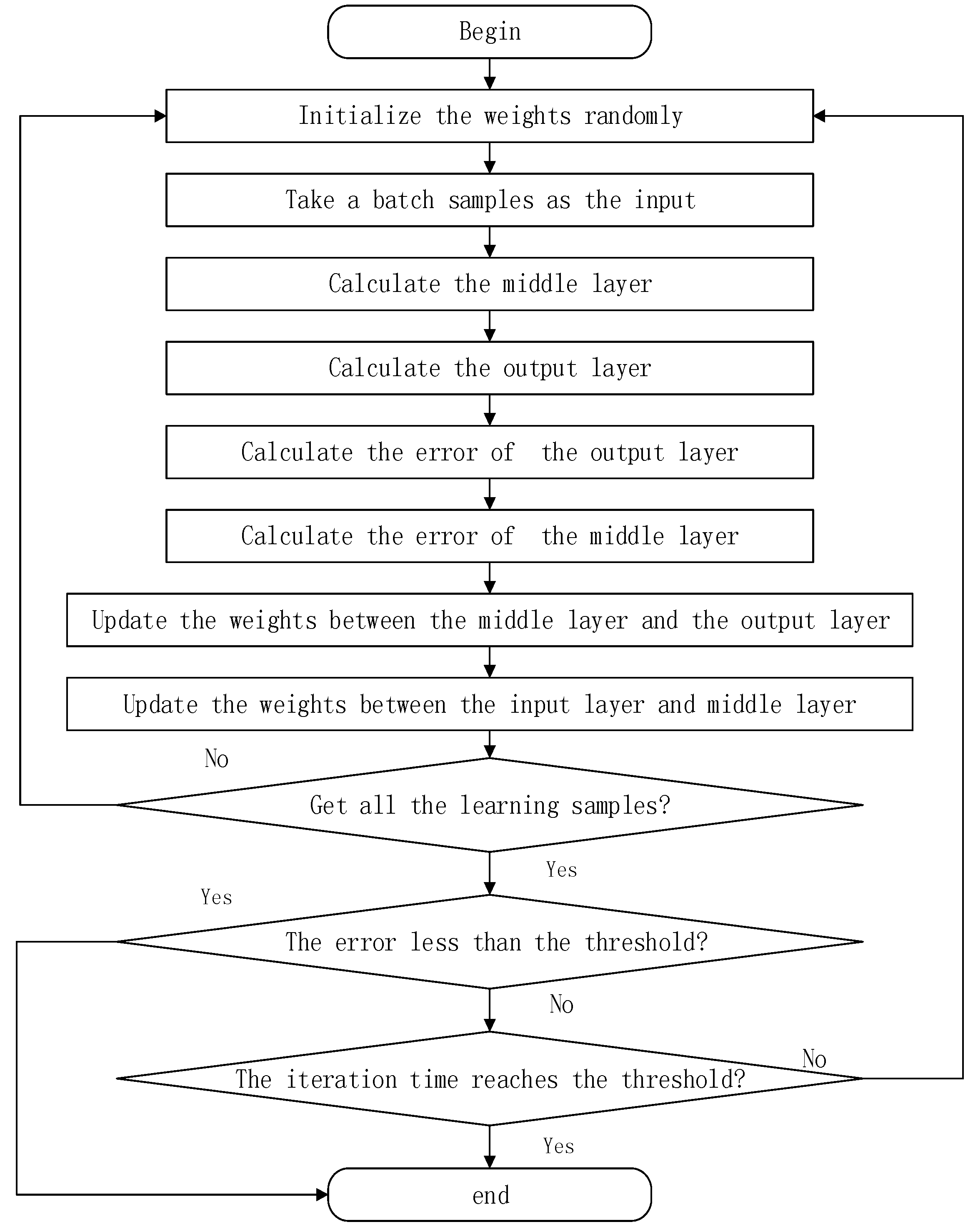
During training, the predicted value is calculated by transmitting it forward through the hidden layer. Then, by comparing the predicted value with the real value, the error is calculated and the weight of each element is modified by back propagation. When the error is less than the threshold, or the iteration time reaches the threshold, the training is stopped. The whole training process is shown in Figure 2.

2.3.3. Click-Through Rate Prediction Based on Multi-Scale Stacking Network

According to user behaviors, product attributes, and advertisement attributes, the multi-scale stacked network model is used to predict whether a user will click on an advertisement, which judges whether a user is a potential high-value customer. The implementation steps of CTR prediction based on the multi-scale stacked network are as follows:
  • The dataset is divided into a training set and a test set. There are different ways to partition different datasets. The datasets that have time can be divided by time, while the datasets without time can be divided by random sampling.
  • To preprocess the dataset, we firstly classify all features with low occurrence times as the same feature while setting a threshold to reduce the dimension of features, which can prevent overfitting to some extent. Secondly, since a numerical feature with a large variance is not conducive for model learning, we carry out log transformation for values greater than 2.
  • The one-hot coding transformation is applied to the classification features, and each feature after the transformation is mapped to an embedded vector with a fixed dimension. All embedded vectors corresponding to the features of a sample are spliced together as the input. The initial value of the embedded vector is set randomly.
  • The MSSP structure is used to construct the high-order and low-order features in different local fields from the depth and width angles.
  • The multi-scale features are fused, and then input to the last prediction layer. Finally, the model outputs the prediction results.
  • The error between the predicted value and the real value is calculated, and the weight of each unit is modified by back propagation. Iterative training is continued to reduce the error until the error is less than the threshold or the iteration times reach the threshold.
  • The learned model is used to predict the test set to find potential high-value customers and guide the distribution of advertisements.

3. Experiments

To objectively evaluate the performance of the proposed algorithm, two public datasets are used in this paper. Both datasets are derived from real advertising data and are the most classic datasets in CTR prediction research. We use two popular metrics, area under the curve (AUC) and log loss, to evaluate the performance of all methods. The experiments are carried out from four aspects. The first aspect is to show the comparison between our MSSP and a model that only mines low-order features. The purpose is to analyze the effectiveness of MSSP in merging low-order and high-order features. The second aspect is to show a comparison of sDeepFM with the DNN module and the current mainstream model, to prove that sDeepFM reaches an advanced level. The third aspect is to discuss the impact of the hyperparameters on the model. The fourth aspect is to discuss the run time efficiency of the model.

3.1. Dataset Description

Criteo: The Criteo dataset comes from a world-renowned internet advertising company whose business focuses on advertising redirection. The data include the user’s personal information, the times the ad was clicked and displayed, the advertising identifier (ID), and other information.
Avazu: The Avazu dataset is derived from the click-through prediction contest published by Avazu on Kaggle in 2015. The dataset consists of 24 columns, all of which are categorical features, and a few of which are numeric ids. Table 1 presents the detailed description of the Criteo and Avazu datasets.

3.2. Evaluation Metrics

AUC: The area under the curve (AUC) is commonly used as a summary measure of the receiver operating characteristic (ROC) curve [18]. As a numerical value, a classifier with a larger AUC is better.
Log loss: Log loss is a commonly used objective function for classification problems, which the model also needs to minimize. We regard it as an intuitive evaluation to measure the effect of the model.
It is worth noting that a 0.001 increase in AUC or a 0.001 decrease in log loss for a CTR prediction task is considered a significant achievement, as mentioned in previous papers [12,15,16].

3.3. Data Preprocessing

To reduce the dimension of the feature and to prevent overfitting to some extent, we classify all the features with less frequency as the same feature set according to their occurrence frequency. The thresholds for classification of Criteo and Avazu were set to {10, 5}, respectively. Secondly, since the numerical properties with large variances are not conducive to learning, we applied a log transformation to the values greater than 2. Thirdly, we randomly selected 80% of the samples for training, and the remaining data were divided into a verification set and a test set. By dividing the data into training, testing, and validation sets, a more consistent stopping criterion could be acquired [19].
For fairness, all our comparison models used the following parameters: (1) dropout 0.5; (2) network structure 400-400; (3) optimizer Adam; (4) activation function Rectified Linear Units (ReLU). In addition, our MSSP has two unique parameters, the stacking deep lever and stacking wide lever. The stacking deep lever was set to 5, and the stacking wide lever was set to the highest order of the two datasets, i.e., 39 in Criteo and 23 in Avazu.

3.4. Experimental Results

3.4.1. Effect of Multi-Scale-Stacking Pooling

This part of experiment was mainly to verify the necessity of higher-order features. The comparison models we adopted, i.e., LR, FM, and AFM, are all models without a deep module. The experimental results are shown in Table 2. Compared with the other models, our model presents great improvement. Our model was superior, mainly because, from multiple perspectives, multi-scale stacking pooling can capture multi-scale features from the first order to the highest order and can effectively integrate high-order and low-order features. In contrast, LR uses only first-order features; FM uses only the first-order and second-order features. AFM adds an attention mechanism to second-order features, but cannot find higher-order features. The experimental results show that it is not enough to learn only low-order features (first-order features and second-order features) and that higher-order features can provide more information for the model, whereby our model learned the higher-order features effectively.

3.4.2. Effect of sDeepFM

Since DNN has certain advantages in exploring high-order implicit information between features, at present, the mainstream models add a deep module. In this part, we further combine the MSSP with the classical DNN to form a unified model named sDeepFM. This part of the experiment is mainly to show a comparison of sDeepFM with the most advanced models at present. As can be seen from Table 3, sDeepFM outperformed all the reference models. Our model shows great improvement over the classical DNN module, which proves the effectiveness of the MSSP module. In comparison, DeepFM integrates FM with DNN, while PNN and xDeepFM construct feature interactions through a product layer, CIN, and multi-head self-attention, before combining with DNN. Unlike the above models, our model sDeepFM determines feature interactions in a completely new way. The experimental results show that our idea is effective and reaches an advanced level. In general, the AUC at 0.7–0.9 indicates that the predicted results have high accuracy. Because of the huge amount of data, even reaching the level of one billion in practical applications, a 0.001 increase in the AUC or a 0.001 decrease in log loss for a CTR prediction task will bring extra millions of dollars each year. Our model improved the results by 0.0014–0.0273 compared with previous models, which can be considered a significant achievement.

3.4.3. Effect of Hyperparameters

  • Effect of stacking width and depth
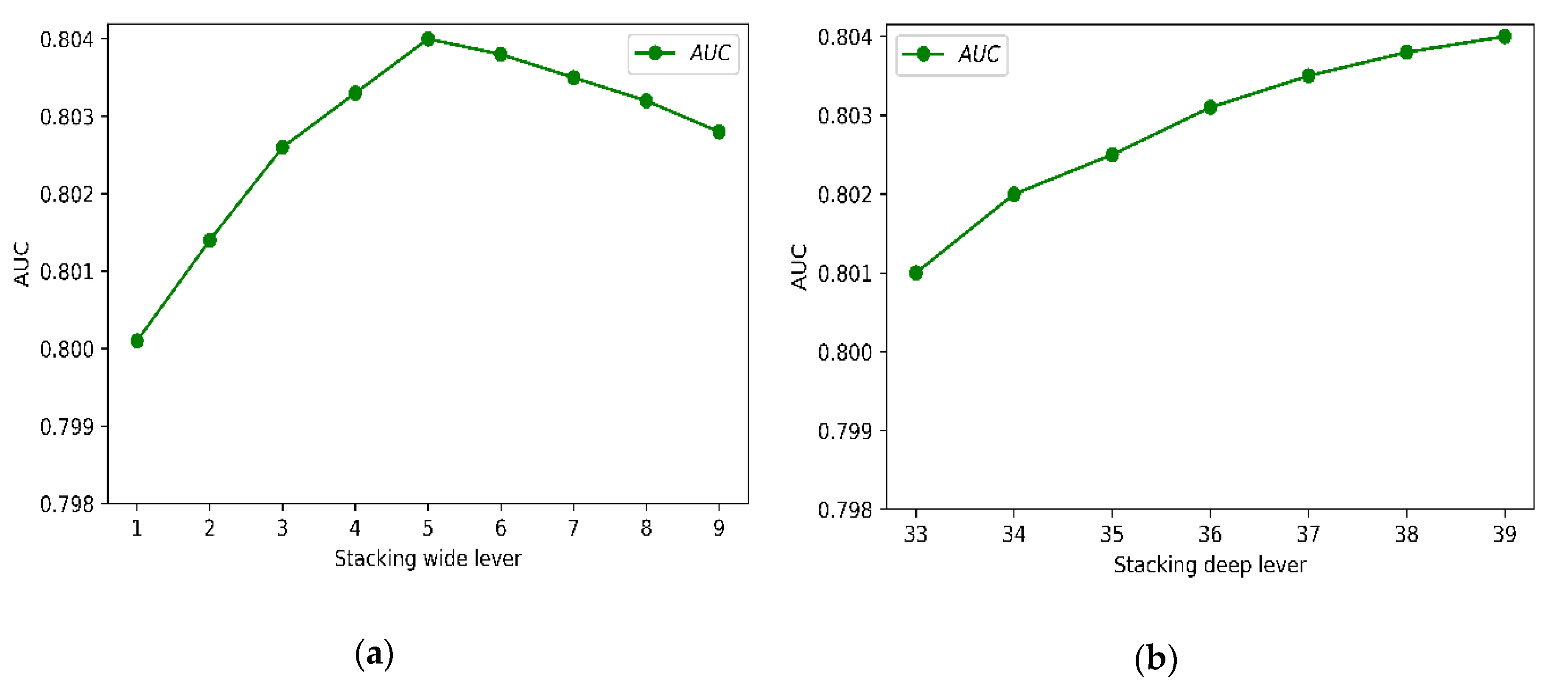
Our model proposed in this paper has two unique parameters, namely, stacking width and depth, which represent the number of detectors and the order of constructed features. Taking the Criteo dataset as an example, we explore the effect of stacking width and depth for MSSP. As shown in Figure 3, when the stacking width was 5 and the stacking depth was 39 (the number of fields in the dataset was also 39), the model reached the optimal result. For stacking deep lever, a higher-order feature results in better performance of the model, which proves that higher-order features can bring useful information to the model. For stacking wide lever, when the order was too high, the model became worse. The reason is that too many MVPs make the model too complex and lead to overfitting.
  • Effect of dropout
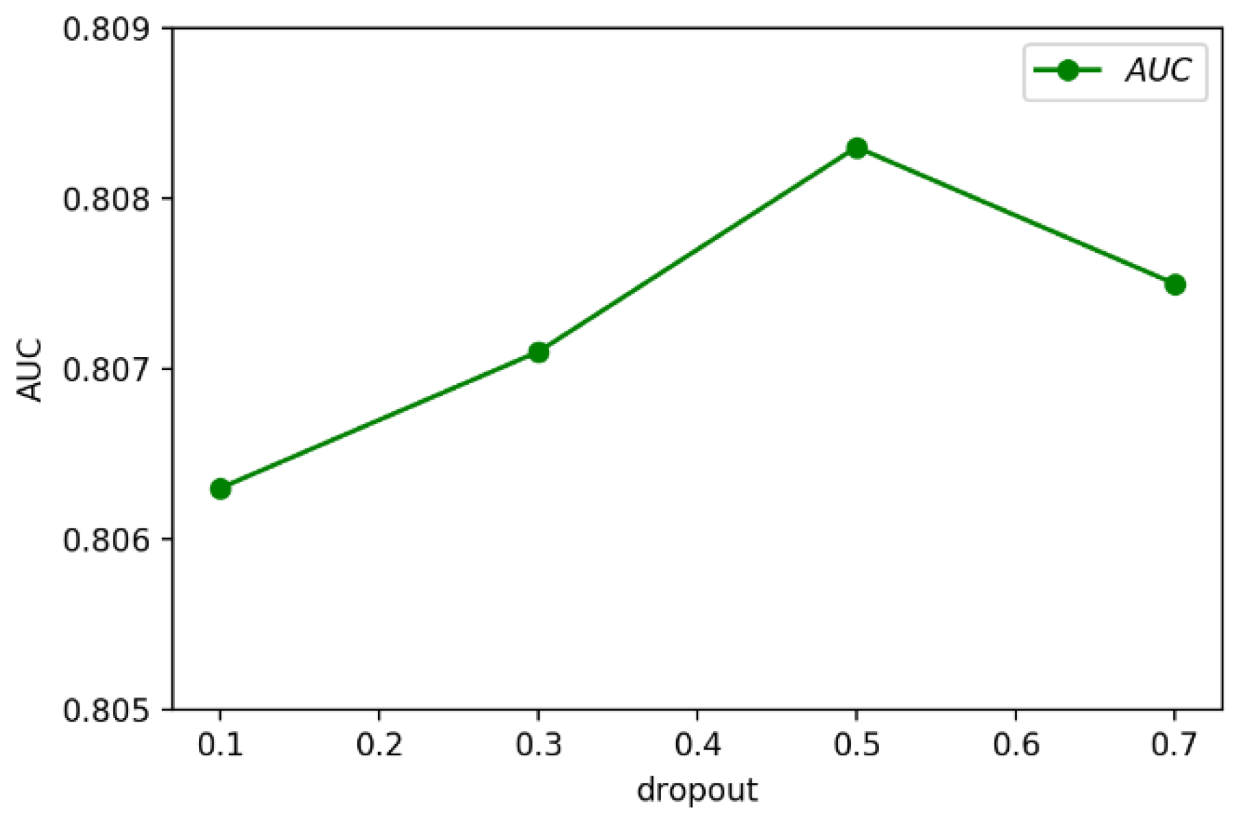
Dropout [20] is a simple and effective regularization method for preventing the model from overfitting, whose mechanism is to stop the neurons of the model working with a certain probability when the model is in the forward propagation stage. Since the neurons which stop working are not exactly the same in each forward propagation stage, the model does not rely too much on local features, thus improving the generalization ability of the model and reducing the risk of overfitting. We explore the effect of dropout on our model by comparing the performance of different dropouts from low to high as 0.1, 0.3, 0.5, and 0.7.
As shown in Figure 4, with the increase in dropout, the AUC of the model increased at first, and then declined when the dropout was greater than 0.5. This is mainly due to the inactivation of too many nodes, which affects the stability of the model. When the dropout was 0.5, only 50% of the neural network nodes were deactivated, and the hidden layer could still learn useful information on a whole. Meanwhile, the parameters and dependencies between nodes were greatly reduced, resulting in the highest AUC. With the further increase in dropout, more and more neurons were deactivated, leading to the disappearance of a large number of dependencies between nodes and a decline in learning ability; thus, the performance of the model worsened.
  • Effect of activation function
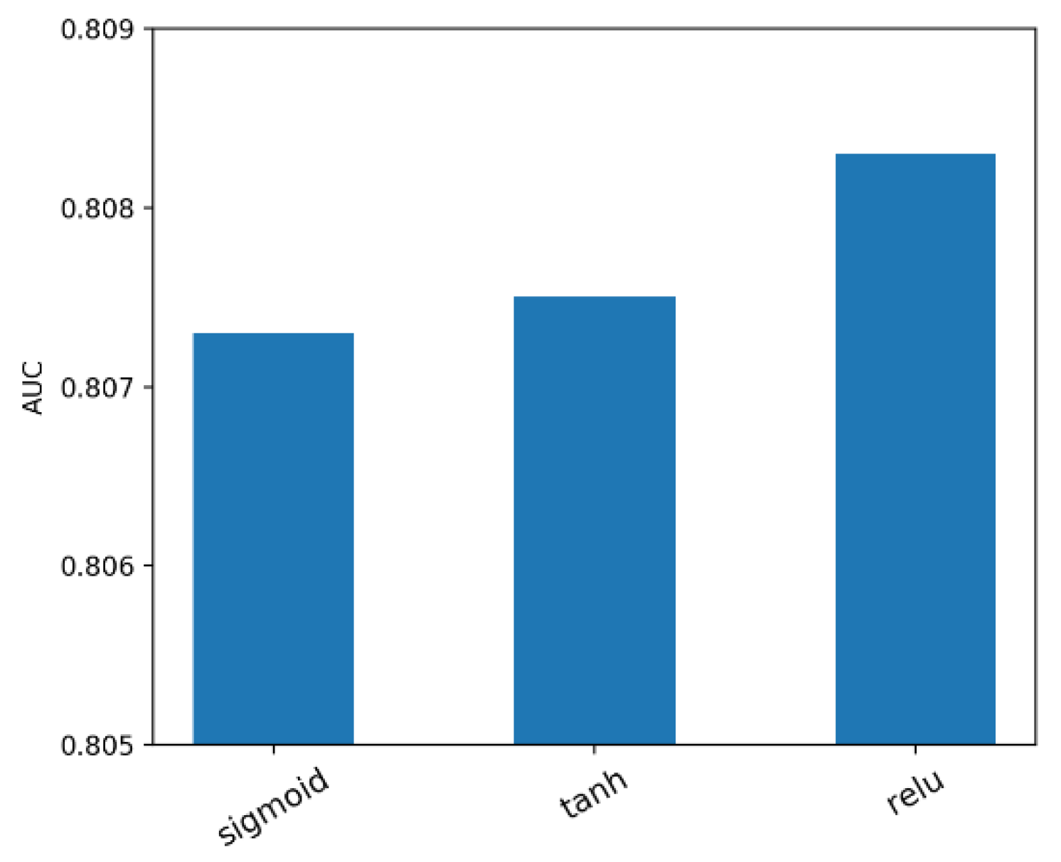
The most important reason for deep neural networks fitting nonlinear data distributions that linear models cannot fit is the existence of an activation function in the neural network. Choosing the appropriate activation function for a deep neural network model can not only avoid the problem of gradient dispersion, but also accelerate the convergence speed of the model and reduce the training time. At present, the common activation functions usually have the properties of piecewise linearity or nonlinearity with an exponential shape such as sigmoid, tanh, and ReLU. As shown in Figure 5, we compared the performance of the model with different activation functions and found that the model with ReLU performed best. Both sigmoid and tanh require an exponential operation, which can slow the calculation speed, facilitating gradient disappearance and gradient explosion. However, the gradient of ReLU is constant when the function is greater than 0, which has a better effect on avoiding gradient dispersion and accelerating the convergence for the model. Therefore, in view of the characteristics of CTR prediction with large input data, the ReLU function is more appropriate for the model than other activation functions, which is demonstrated in our experiment.
  • Effect of number of neurons
Increasing the number of neurons per layer can add to the complexity of the model. We compared the performance of our model with different numbers of neurons. As shown in Figure 6, increasing the number of neurons was not always beneficial. With the increase in the number of neural units, the performance of the model was initially improved. However, upon reaching a certain threshold, if the number of neural units continued to increase, the model became too complex, thus leading to overfitting and difficulty in optimization, thereby degrading the performance to some extent.

3.4.4. Discussion of Run Time Efficiency

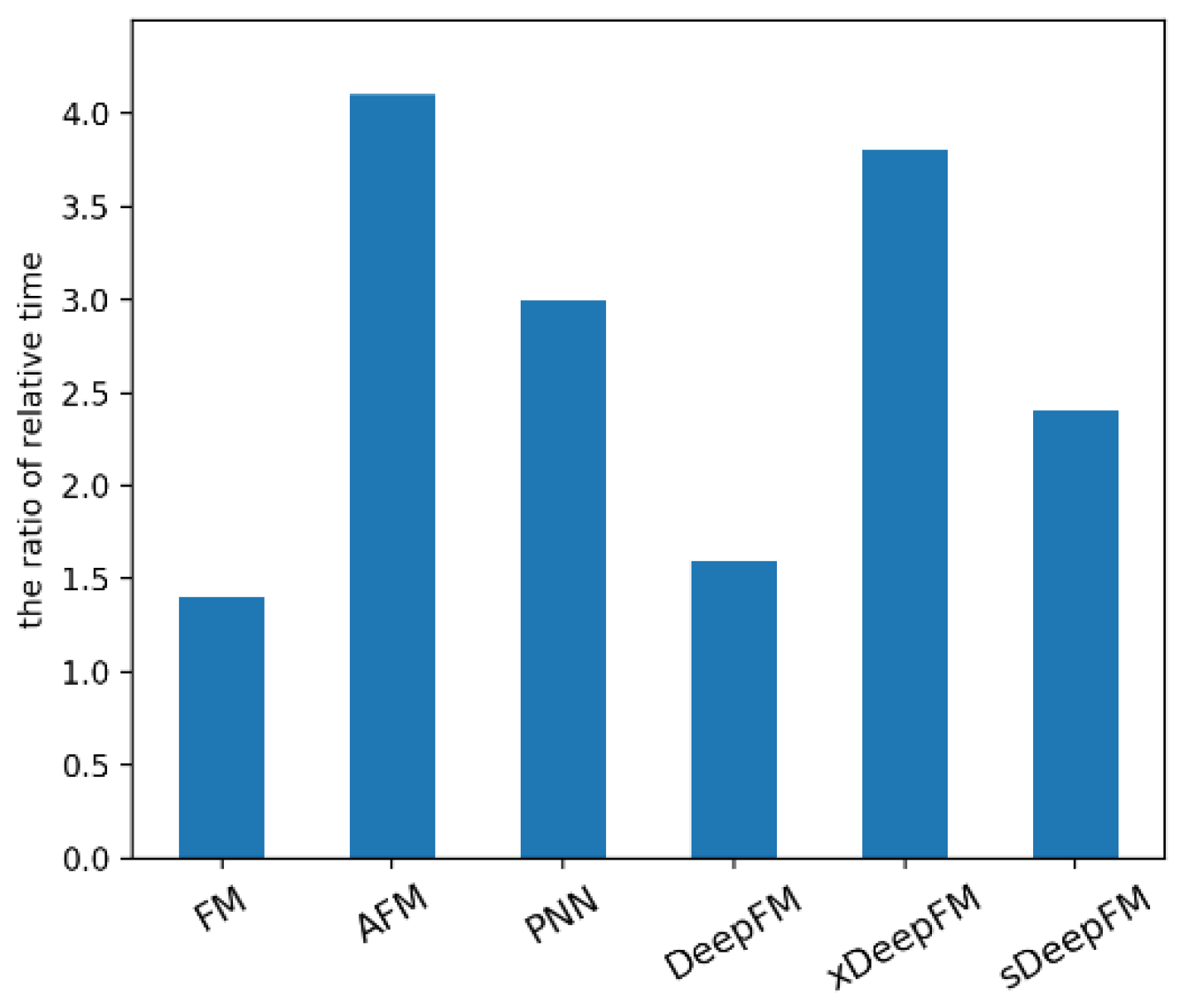
The training process of deep learning usually requires a lot of time and computing resources, which is an important reason for the development of deep learning. Since a real business scenario is oriented toward massive data, the training speed of the deep neural network is crucial for the implementation of algorithms. In this section, we compare the training efficiency of different models on the Criteo dataset by using the ratio of relative time calculated by the following formula: Tdl/Tlr, where Tdl and Tlr are the training time of the deep learning model and logistic regression model, respectively. The graphics card we used for training was Tesla P100. As shown in Figure 7, the abscissa represents the name of the models, while the ordinate shows the ratio of relative time. We can conclude that AFM required the longest training time, followed by xDeepFM and PNN, then our model, and finally DeepFM and FM. Gains of AUC performance and model complexity need to be achieved at the cost of time. Our model was slightly slower than the fastest FM within an acceptable range, but the enhancement of AUC was relatively large. Compared with AFM, xDeepFM, and PNN, the AUC and time performance were both improved.

4. Conclusions

In this paper, we proposed multi-scale stacking pooling based on different receptive fields for extracting multi-scale features, which mines the high-order and low-order features in different local fields with bidirectional stacking of the multi-view features from depth and width. The structure is an effective way of combining low-order and high-order features to ensure the diversity of extracted features. Through the exploratory research of real data, this paper confirmed the necessity of fusing high-order features and low-order features. Moreover, parameter factorization resulted in the cross terms being no longer independent of each other, ensuring that the high-order features could be effectively learned in sparse data. We also made a meaningful exploration of the hyperparameters of sDeepFM. On two public datasets, our model outperformed the state-of-the-art models. Our method of multi-scale stacking pooling is a transplantable operation, and other neural networks can refer to our structure and further innovate it, which has certain significance for future research. Furthermore, we are now entering the era of data, where mining the information of user data can bring great value to enterprises. Thus, this will be a hot topic for future academic and industrial research.
Due to the limited experimental research conditions, this work is still limited. The research of deep learning in CTR prediction is not deep enough. Neural networks have the disadvantage of being sensitive to initial weights, and unsupervised pre-training can improve this shortcoming. How to use unsupervised learning, using some common unsupervised modules such as auto encoder and restricted Boltzmaner, to optimize the initial DNN in CTR prediction problems is an interesting topic. Furthermore, the attention mechanism is currently a hot direction. How to integrate the advanced attention method into our model is a subject worth studying.

Author Contributions

B.Q. provided the methodology for our project. Y.L. carried out the formal analysis. M.Y. guided the paper. X.C. helped with modeling and validation. J.C. was responsible for the conceptualization of our project. Y.C. wrote the code for the software and designed the validation experiments. All authors have read and agreed to the published version of the manuscript.

Funding

This work was partially supported by the National Natural Science Foundation of China (61762025), the Guangxi Key Research and Development Program (AB17195053, AB18126053), the Natural Science Foundation of Guangxi of China (2017GXNSFAA198226, 2019GXNSFDA185007), Guilin Science and Technology Development Program (20180107-4), the Innovation Project of GUET Graduate Education (2019YCXS051), and the Guangxi Colleges and Universities Key Laboratory of Intelligent Processing of Computer Image and Graphics (No. GIIP201603).

Conflicts of Interest

The authors declare no conflicts of interest.

References

  1. Covington, P.; Adams, J.; Sargin, E. Deep neural networks for Youtube recommendations. In Proceedings of the 10th ACM Conference on Recommender Systems, New York, NY, USA, 15–19 September 2016; pp. 191–198. [Google Scholar]
  2. He, X.; Pan, J.; Jin, O.; Xu, T.; Liu, B.; Xu, T.; Candela, J.Q. Practical lessons from predicting clicks on ads at facebook. In Proceedings of the Eighth International Workshop on Data Mining for Online Advertising, New York, NY, USA, 24 August 2014; pp. 1–9. [Google Scholar]
  3. Richardson, M.; Dominowska, E.; Ragno, R. Predicting clicks: Estimating the click-through rate for new ads. In Proceedings of the 16th International Conference on World Wide Web, Banff, AB, Canada, 8–12 May 2007; pp. 521–530. [Google Scholar]
  4. Domingos, P. A few useful things to know about machine learning. Commun. ACM 2012, 55, 78–87. [Google Scholar] [CrossRef] [Green Version]
  5. Rendle, S. Factorization machines with libfm. ACM Trans. Intell. Syst. Technol. 2012, 3, 1–22. [Google Scholar] [CrossRef]
  6. Shan, Y.; Hoens, T.R.; Jiao, J.; Wang, H.; Yu, D.; Mao, J.C. Deep crossing: Web-scale modeling without manually crafted combinatorial features. In Proceedings of the 22nd ACM SIGKDD International Conference on Knowledge Discovery and Data Mining, San Francisco, CA, USA, 22 September 2016; pp. 255–262. [Google Scholar]
  7. Chang, Y.W.; Hsieh, C.J.; Chang, K.W.; Ringgaard, M.; Lin, C.J. Training and testing low-degree polynomial data mappings via linear svm. J. Mach. Learn. Res. 2010, 11, 1471–1490. [Google Scholar]
  8. Rendle, S.; Schmidt-Thieme, L. Pairwise interaction tensor factorization for personalized tag recommendation. In Proceedings of the Third ACM International Conference on Web Search and Data Mining, New York, NY, USA, 3–6 February 2010; pp. 81–90. [Google Scholar]
  9. Juan, Y.; Zhuang, Y.; Chin, W.S.; Lin, C.J. Field-aware Factorization Machines for CTR Prediction. In Proceedings of the ACM Conference on Recommender Systems, Boston, MA, USA, 15–19 September 2016. [Google Scholar]
  10. Wang, G.; Li, Q.; Wang, L.; Zhang, Y.; Liu, Z. Elderly fall detection with an accelerometer using lightweight neural networks. Electronics 2019, 8, 1354. [Google Scholar] [CrossRef] [Green Version]
  11. Zhang, C.; Fu, Y.; Deng, F.; Wei, B.; Wu, X. Methane Gas Density Monitoring and Predicting Based on RFID Sensor Tag and CNN Algorithm. Electronics 2018, 7, 69. [Google Scholar] [CrossRef] [Green Version]
  12. Cheng, H.-T.; Koc, L.; Harmsen, J.; Shaked, T.; Chandra, T.; Aradhye, H. Wide & deep learning for recommender systems. In Proceedings of the 1st Workshop on Deep Learning for Recommender Systems, Boston, MA, USA, 15 September 2016; pp. 7–10. [Google Scholar]
  13. Zhang, W.; Du, T.; Wang, J. Deep learning over multi-field categorical data: A case study on user response prediction. In Proceedings of the European Conference on Information Retrieval, Padua, Italy, 20–23 March 2016; pp. 45–57. [Google Scholar]
  14. Qu, Y.; Cai, H.; Ren, K.; Zhang, W.; Yu, Y.; Wen, Y.; Wang, J. Product-based neural networks for user response prediction. In Proceedings of the IEEE 16th International Conference on Data Mining, Barcelona, Spain, 12–15 December 2016; pp. 1149–1154. [Google Scholar]
  15. Xiao, J.; Ye, H.; He, X.; Zhang, H.; Wu, F.; Chua, T.S. Attentional Factorization Machines: Learning the Weight of Feature Interactions via Attention Networks. arXiv 2017, arXiv:1708.04617. [Google Scholar]
  16. Guo, H.; Tang, R.; Ye, Y.; Li, Z.; He, X.; Dong, Z. DeepFM: An end-to-end wide & deep learning framework for CTR prediction. arXiv 2018, arXiv:1804.04950. [Google Scholar]
  17. Lian, J.; Zhou, X.; Zhang, F.; Chen, Z.; Xie, X.; Sun, G. Xdeepfm: Combining explicit and implicit feature interactions for recommender systems. In Proceedings of the 24th ACM SIGKDD International Conference on Knowledge Discovery & Data Mining, London, UK, 19–23 August 2018; pp. 1754–1763. [Google Scholar]
  18. Walter, S.D. The partial area under the summary ROC curve. Stat. Med. 2005, 24, 2025–2040. [Google Scholar] [CrossRef] [PubMed]
  19. Abbas, F.; Feng, D.; Habib, S.; Rahman, U.; Rasool, A.; Yan, Z. Short term residential load forecasting: An improved optimal nonlinear auto regressive (narx) method with exponential weight decay function. Electronics 2018, 7, 432. [Google Scholar] [CrossRef] [Green Version]
  20. Srivastava, N.; Hinton, G.; Krizhevsky, A.; Sutskever, I.; Salakhutdinov, R. Dropout: A simple way to prevent neural networks from overfitting. J. Mach. Learn. Res. 2014, 15, 1929–1958. [Google Scholar]
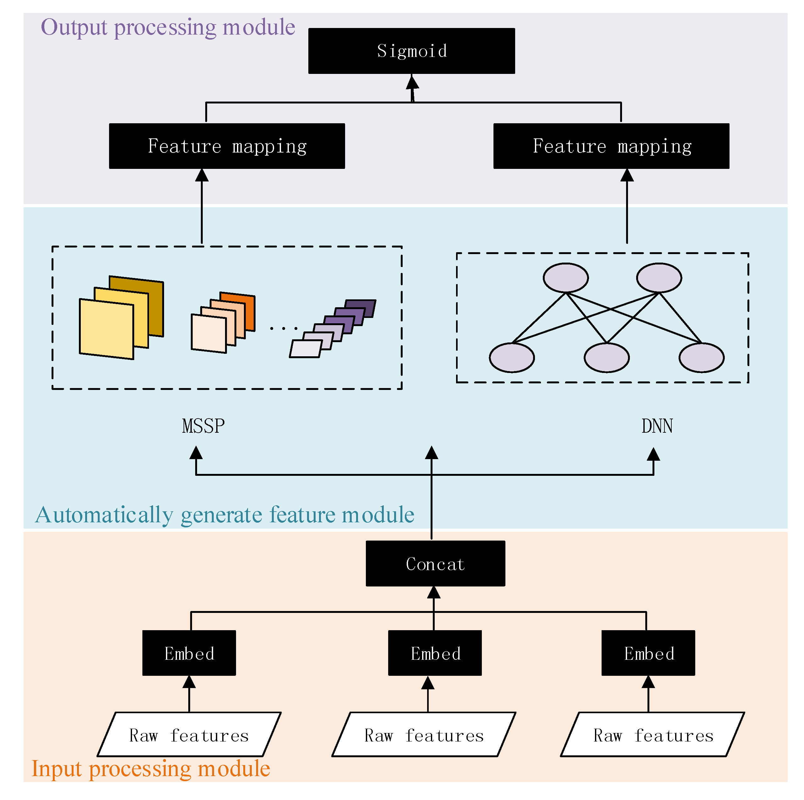
Figure 1. The whole structure of sDeepFM.
Electronics 09 00350 g001
Figure 2. Process of model training.
Electronics 09 00350 g002
Figure 3. (a) Description of effects of stacking width lever; (b) description of effects of stacking deep lever.
Electronics 09 00350 g003
Figure 4. The impact of dropout on the model.
Electronics 09 00350 g004
Figure 5. The impact of activation function on the model.
Electronics 09 00350 g005
Figure 6. The impact of the number of neurons on the model.
Electronics 09 00350 g006
Figure 7. The run time efficiency of the models.
Electronics 09 00350 g007
Table 1. The statistics of Criteo and Avazu.
DataSamplesFieldsFeatures
Criteo45,840,61739998,960
Avazu40,428,967231,544,488
Table 2. Comparison of multi-scale stacking pooling (MSSP) with other models without a deep neural network (DNN) module. LR—logistic regression; FM—factorization machine; AFM—attentional factorization machine; AUC—area under the curve.
CriteoAvazu
AUCLog LossAUCLog Loss
LR0.78100.46900.75880.3962
FM0.78230.46880.77010.3855
AFM0.79400.45800.77150.3853
MSSN0.80400.44740.77440.3829
Table 3. Comparison of MSSP with other models without a DNN module. PNN—product-based neural network.
CriteoAvazu
AUCLog LossAUCLog Loss
DNN0.80060.45200.77300.3850
PNN0.80380.44830.77500.3827
DeepFM0.80500.44750.77510.3829
xDeepFM0.80690.44520.77630.3819
sDeepFM0.80830.44360.77710.3811