1. Introduction
The ever-declining petroleum resources have forced worldwide nations to optimize the energy mix for sustainable development. In the global search for clean, renewable and safe energy sources, solar power is most concerned due to its ubiquitous existence, inexhaustible amount, and high-level safety. The past decade has witnessed tremendous growth in the global photovoltaic market, and this trend is still continuing. At the end of 2019, the world’s total photovoltaic capacity has reached 580 GW, which is increased by 20.1% compared with 2018 [
1]. In China, it is expected that the cumulative installed photovoltaic capacity will be rocketed from 130 GW by 2017 [
2] to approximately 2.7 TW by 2050 [
3].
Despite the fast growth rate, photovoltaic systems are still confronted with the challenge of enhancing efficiency. Solar cells typically exhibit nonlinear power–voltage curves [
4], and are very sensitive to external conditions [
5]. Given the invariably changing irradiance and temperature, it is crucial to keep all solar cells generating at maximal power point (MPP) so as to enhance the conversion efficiency of photovoltaic systems. To this end, various maximal power point tracking (MPPT) techniques have been presented, displaying different features including accuracy, tracking speed, algorithm complexity, steady-state oscillation, hardware installation, and cost [
6,
7,
8,
9,
10,
11].
Direct methods such as Perturb and Observe (P&O) and Incremental Conductance (InC) have been proposed to directly calculate the MPP. In the P&O method, the control unit will slightly increase or decrease the output voltage, measuring and comparing output power until MPP is reached. The InC method calculates MPP by comparing incremental conductance and module conductance. Both methods offer good extendibility to different scales of photovoltaic systems, but are of limited dynamic response and is susceptible to oscillation around the MPP [
12]. In both methods, the perturbation step size is a key parameter, as a small step size lowers tracking speed but a large step size reduces tracking accuracy [
13]. As a trade-off, the variable step size has been presented. For instance, a two-stage algorithm is incorporated into the P&O method to achieve coarse tracking in the first stage and fine tracking in the second stage to reduce response time [
14]. In a variable step size InC method, direct control of the scaling factor is proposed to increase the speed of convergence while maintaining tracking accuracy [
15]. However, the steady-state oscillation problem is still not completely excluded. Moreover, under asymmetrical conditions such as hot-spotting or partial shading, both methods cannot guarantee effective tracking of global MPP [
16].
Recently, a variety of algorithm-based MPPT methods (a.k.a. soft MPPT methods) have been presented, including artificial neural networks (ANN) [
17,
18,
19,
20,
21], fuzzy logic (FL) [
22,
23,
24], grey wolf [
25], artificial bee colony [
26], particle swarm optimization (PSO) [
27,
28,
29,
30], etc. These methods provide robust and versatile performance, and are generally capable of tracking global MPP under various conditions. For ANN methods, MPP voltage is accurately calculated through improved network architecture such as back-prorogation network [
17] and radial basis function network [
18], or through optimization algorithms such as genetic algorithm [
19] and gradient descent momentum algorithm [
20]. By incorporating the auto-scaling method into the FL controller, fast transient tracking speed and good convergence around MPP are jointly achieved [
22]. Based on a PSO algorithm featured by reducing swarm size, global MPP has been tracked with fast convergence speed under partial shading conditions [
27]. However, these methods usually require complex mathematical models and calculations, and the effectiveness of these methods usually relies on careful selection of model parameters or massive data training in advance. For instance, the ANN MPPT adopted in [
21] registered training with data obtained in one year. The membership function in FL MPPT also requires sufficient experiments and modifications to be built properly [
23]. Upon a sharp change of photovoltaic system characteristics or ambient conditions, these methods also require more time to learn and to adapt [
31].
On the contrary, fractional open-circuit voltage (FOCV) is a widely adopted MPPT method in practice due to its low calculation complexity, easy implementation and cost-effectiveness [
32,
33,
34]. Though it tracks MPP in an indirect way, it has fast-tracking speed and minimal requirements of sensors, and is of comparable accuracy in most situations [
35]. The main problem of the FOCV method is the disturbed output power due to the common practice of disconnecting PV panel from the load during open-circuit voltage measurement. This measuring period not only results in temporal loss of power, but also affects the accuracy of tracked MPP. To solve this problem, methods such as pilot cell [
36] and semi pilot cell [
37] have been proposed, in which pilot cells are used for measuring open-circuit voltage. For these two methods, the representativeness of the pilot cells is a big issue, esp. in non-uniform insolation conditions. In addition, the semi pilot cell method results in increased ripple of output power. In order to realize interruption-free output power, an online FOCV method has been proposed [
38]. The open-circuit voltage is calculated through a model based on the results of multiple sensors, including current, voltage and temperature, which increases complexity in both calculation and hardware implementation.
In this paper, we present an improved traversal FOCV method with easy implementation and uninterrupted output power. The open-circuit voltage of each solar cell is measured on-site through consecutively switching in or out, solving the representativeness issue. Meanwhile, the output power is not disturbed as the number of power generating cells remains constant. The proposed method will be explained in detail in the following sections, and will be compared with the pilot cell and semi pilot cell methods in both time-varying irradiance and spatial-varying irradiance conditions.
2. Proposed Method
The traditional fractional open-circuit voltage method is based on the approximation that the MPP voltage has a linear relationship with open-circuit voltage. The whole panel is connected with the load in the powering session, and is disconnected from the load in the tracking session to measure open-circuit voltage and estimate MPP of the whole panel. This method has two problems: (1) MPP is estimated for the whole panel rather than specific solar cells; (2) during the tracking session the power loss is 100% and fluctuations are inevitable.
One improving method is the pilot cell (PC) method, in which an individual pilot cell is set aside on the photovoltaic panel, as is shown in
Figure 1a. The pilot cell can be tested periodically or continuously, while the remaining solar cells generate power to the load. It avoids power loss of the whole photovoltaic panel while open-circuit voltage measurement is in process. However, the problem still exists in that electrical characteristics of the pilot cell may not be representative of all solar cells in the system, and thus the calculated MPP might not be accurate for the entire photovoltaic panel.
Another improving method is the semi pilot cell (SPC) method. As is shown in
Figure 1b, a selected semi-pilot cell is either connected with an antiparallel bypass diode (Path ①) to generate power with other solar cells on the panel, or connected with a voltage sensor (Path ②) for open-circuit voltage measurement. In the latter condition, the bypass diode turns on to maintain the current on the panel. The semi-pilot cell method increases output power for small-scale photovoltaic systems, but the changing amount of generating solar cells increases the fluctuation of generated power. Still, the measured open-circuit voltage of the chosen semi-pilot cell is not representative of all solar cells in the photovoltaic panel.
The presented on-site traversal fractional open-circuit voltage method is shown in
Figure 2. Each solar cell was connected with a bypass diode and a couple of reverse single pole double throws (SPDTs). Here, Schottky diodes were selected as bypass diodes for their low forward voltage drop and high switch frequency, which was suitable for the fast switching in and out in the proposed method. In the SPDTs, Point 1 was connected with the specific solar cell. Point 2 was connected with other cells in the panel in series. Point 3 was connected with the voltage sensor. Only one voltage sensor was needed in the proposed method, as it was shunt with Point 3 of all SPDTs. Assuming that the total amount of solar cells is N in the photovoltaic system, the proposed method operates as follows:
- (1)
The mth solar cell (m = 1, 2, ..., N−1) is connected with voltage sensor through Point 3 for open-circuit voltage measurement, while all other N − 1 solar cells are connected to load through Point 2 and are generating power.
- (2)
SPDTs of the mth solar cell and the (m + 1)th solar cell changes simultaneously. For the mth solar cell, SPDTs switch from Point 3 to Point 2. For the (m + 1)th solar cell, SPDTs switch from Point 2 to Point 3.
- (3)
After the switch change in (2), the mth solar cell is connected to the panel for power generation, while the (m + 1)th solar cell is connected with voltage sensor for open-circuit voltage measuring.
- (4)
This process proceeds as all solar cells in the panel are measured in the traversal.
In the proposed method, every independent solar cell owns its non-overlapping measurement window phase with equal time length Δ
t. The operation cycle
T of the entire system is:
For simplicity, assume that the output voltage of a single cell is
u0(
t). Throughout the entire cycle T, the output voltage of the panel to the load
uout(
t) is:
It can be seen from Equation (2) that, constant number of generating solar cells is the key to reduced ripple and stable output. The fast switching speed of power electronics enables real-time measurement for the open-circuit voltage of each solar cell, and since the measurement is performed on-site rather than representatively, the obtained MPP of the whole panel is more accurate compared with the PC method or SPC method.
For large scale photovoltaic systems, the principle of the proposed method can also be extended to implement on a solar panel scale. In this circumstance, each panel serves as an independent unit for measuring open-circuit voltage and determining local MPP. Compared with solar cell scale implementation, which usually requires on-chip integrated electronics, processing and control on the solar panel scale can be achieved via circuit boards, which offers more flexibility and better compatibility for existing systems.
Regardless of cell scale or panel scale implementation, the proposed method provides the feasibility that all units can be specifically controlled using SPDTs. Based on this, the measuring sequence can be further extended as sequential, random, or depending on the task. Such a feature is especially helpful when combined with distributed sensing of environmental conditions, e.g., when a hot spot or shaded spot has been sensed, the location-specific solar cell/panel can be instantly on-site measured to adjust the MPP of the whole system.
3. Modeling of Solar Cells
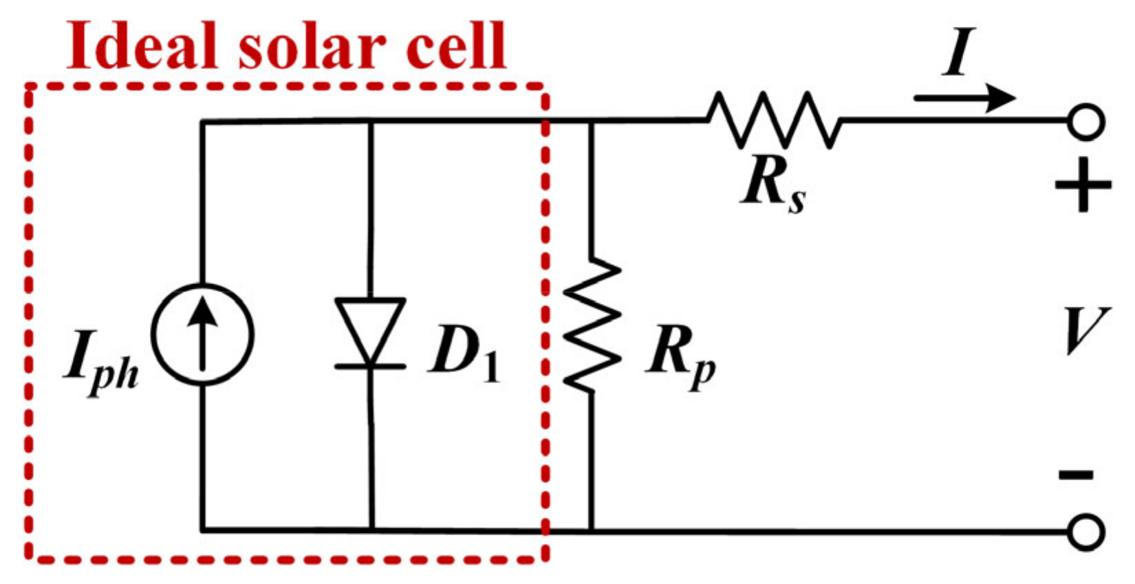
The practical solar cell is usually modeled as an ideal solar cell with parallel and serial resistances. As is shown in
Figure 3,
Iph is the ideal current source,
D1 is the inherent diode,
Rp represents leakage current, and
Rs represents the internal power loss due to current flow.
The
I-
V relation of
Figure 3 is described as:
where
I is the output current of the solar cell,
Vt is the thermal voltage of the diode and is equal to
kT/
q, in which
k is the Boltzmann constant,
q is the electron charge, and
T is the junction temperature in Kelvin.
Is is the diode reverse saturation current,
N is the quality factor of the diode, and
V is the output voltage of the solar cell.
Assuming that
Rp is infinite and
Rs = 0, Equation (3) can be simplified as:
In open-circuit condition
I = 0, so Equation (4) can be rewritten as:
where
Voc is the open-circuit voltage of the solar cell.
Denoting
γ as the ratio between
Iph and
Is:
Output current
I can be obtained from Equations (3), (5) and (6):
Since γ >> 1, the general trend depicted in Equation (7) is that I decreases as V increases. Maximally when V = Voc, the output current I is zero.
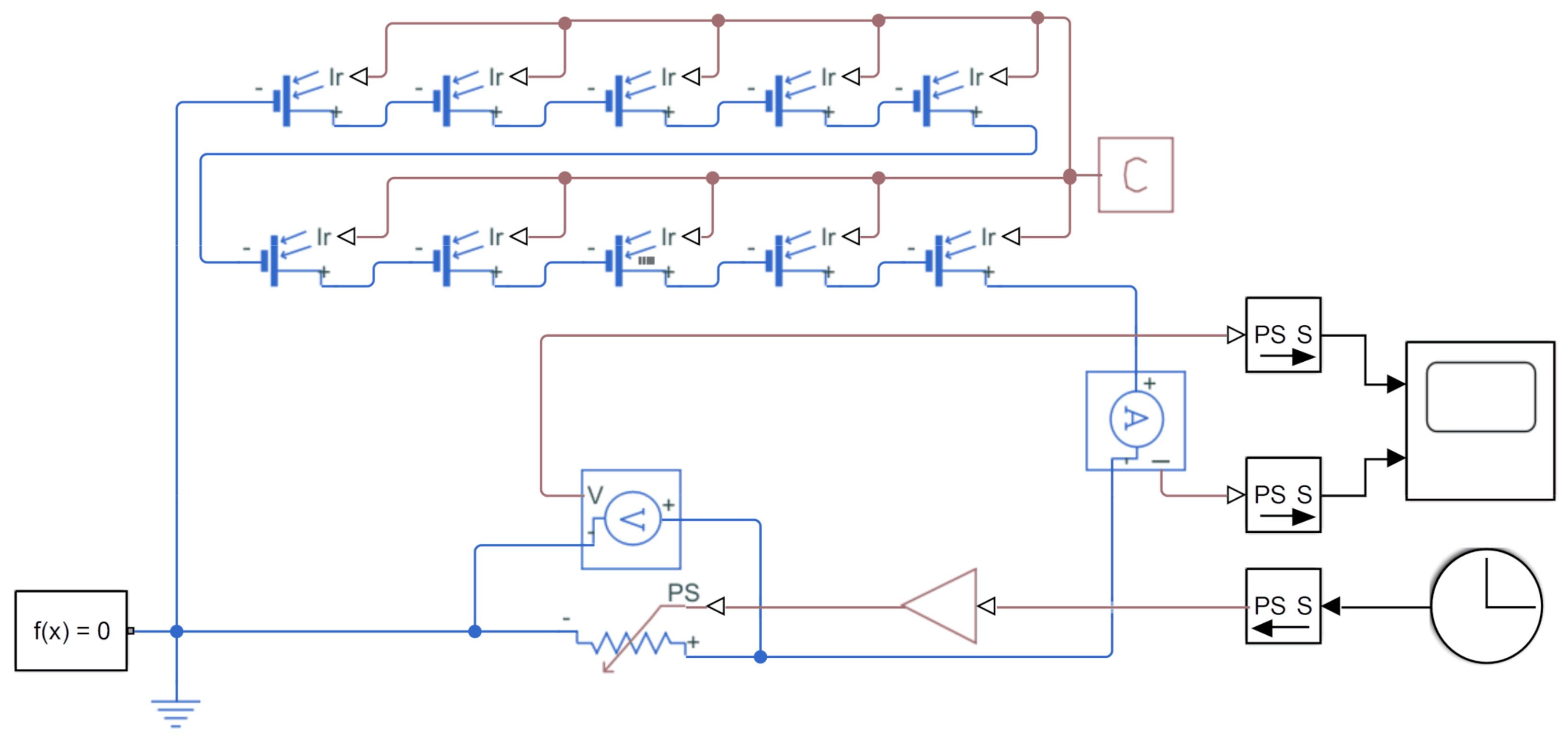
The output performance of solar cells is simulated using MATLAB/Simulink, and the testing circuit is shown in
Figure 4. The circuit consists of ten solar cells in series whose input irradiance
Ir is given by a constant irradiance
C. The parameters of the solar cells are:
Voc = 0.6 V,
Isc = 6 A. The load resistance is increasing with time from 0 to a finite value to collect data from short-circuit status to almost open-circuit status. Solar irradiance is set as 1000, 800, 600, 400 and 200 W/m
2, and ambient temperature is set as 0, 25, and 50 °C, respectively.
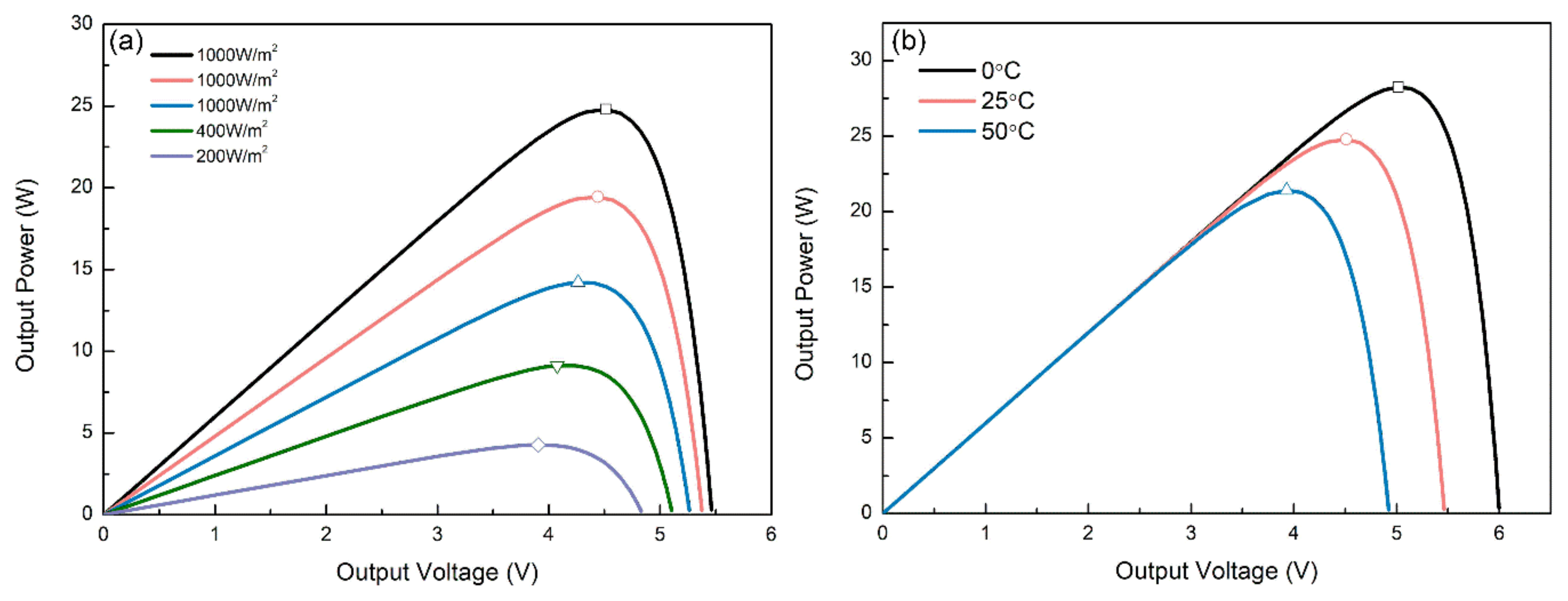
The simulated
P-
V curves of the solar cells under different irradiations and temperatures are shown in
Figure 5. For
Figure 5a, the temperature was set to 25 °C, while for
Figure 5b, the irradiance was set as 1000 W/m
2. It can be seen clearly that MPP drifts with irradiations and temperatures. The output power increased with increasing solar irradiance but decreased with increasing temperature. Since output power changed more conspicuously under different light irradiance than under different temperatures, the following simulation works were majorly focused on different light irradiance.
In a photovoltaic system, the MPP voltage
Vmpp of the solar cell keeps an approximately linear relationship to its open-circuit voltage
Voc:
where
k is a proportionality factor, and is mainly decided by characteristics of the solar cell instead of environmental conditions. Usually,
k is in the range of [0.75, 0.85].
Based on the simulation results of
Figure 5, the relationship between solar irradiance
Ir,
Voc,
Vmpp, and
k is shown in
Table 1. Subsequently,
k is set to be the average value of 0.81 in the following circuit simulation.
4. Circuit Simulation
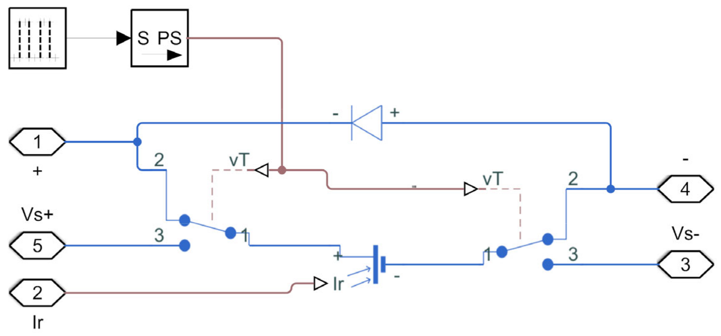
Based on the above solar cell model,
Figure 6 shows the schematic of an independent unit, consisting of a solar cell, a couple of reverse SPDTs, and a bypass diode. The connection method of these three components is the same as
Figure 2. The entire unit had five ports. Ports 1 and 4 were the anode and cathode of this unit, which is for serial connection with other units in the main circuit. Ports 3 and 5 were the open-circuit voltage measurement ports, which were connected to the voltage sensor. Port 2 is the light irradiance input. The two SPDTs were under the control of a common input pulse for the aim of synchronous switch operation. The solar cell was connected with other units when SPDTs were turned to Point 2, or connected with the voltage sensor when SPDTs were turned to Point 3.
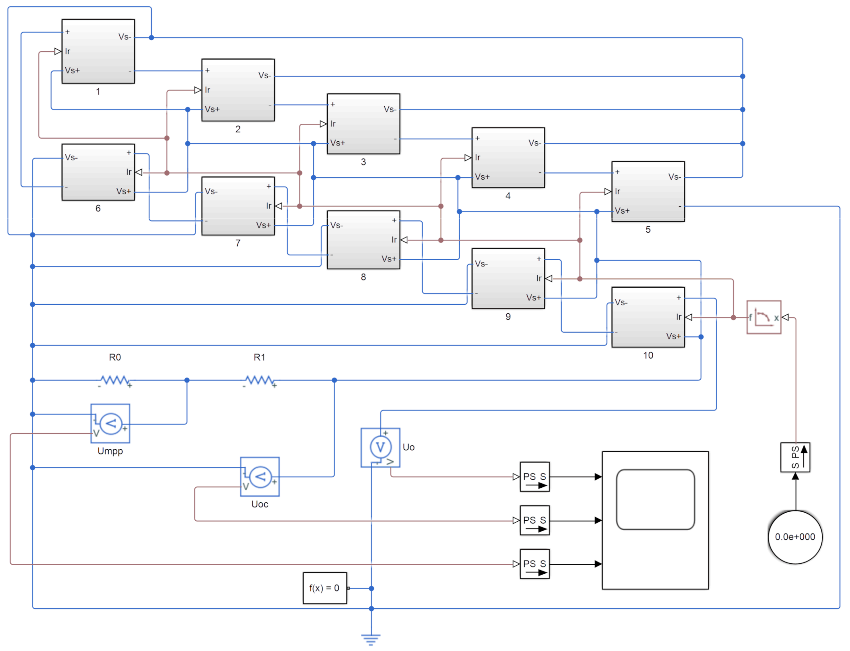
The independent unit in
Figure 6 is packaged into a block, and in
Figure 7, 110 such blocks are shown. The ports on the encapsulated block correspond to ports in a single unit. Port 1 (+) and Port 4 (−) in all blocks were connected in series, so that if SPDTs were turned to Point 2, all solar cells cascaded. Port 3 (Vs−) and Port 5 (Vs+) in all blocks were connected in parallel, so that if one couple of SPDTs was turned to Point 3, the solar cell connected with the SPDTs was shunt with the voltage sensor for MPP calculation. Voltage sensor U
o measured the output voltage of the whole system. Voltage sensors U
oc and U
mpp measured the open-circuit voltage and MPP voltage of the testing cell, respectively. The resistance value of
R0 and
R1 satisfy the expression of
R0/(
R0+
R1) =
k, so that open-circuit voltage and MPP voltage are in accordance with Equation (8). The measured MPP voltage can be transferred to subsequent DC–DC converters to achieve maximum output power. The ten couples of SPDTs in the blocks are controlled by sequential pulses, so that the solar cells in Blocks 1–10 are consecutively connected to the voltage sensor for open-circuit voltage measuring.
In order to compare the proposed method with the conventional PC method and SPC method, two case studies were applied. One was the time-varying irradiance case, in which all solar cells were subject to the same irradiance varying with time. The other was the spatial-varying irradiance case, in which solar cells were subject to constant but different irradiance according to their respective location.
In the time-varying irradiance case,
Figure 8a shows the typical solar irradiance curve from 0 to 24 h, which is set as the environmental condition. The curve rose above zero after 4 h, reached a maximum of 1000 W/m
2 at 12.27 h, and fell to zero after 20 h. The time period 9–15 h contained 70.7% of total solar irradiance, and 11–13 h contained 40.0% of total solar irradiance. Thus, the following comparison of simulation results is majorly conducted in these two time periods.
Figure 8b shows the output voltage of SPC method, the time-varying trend of which is in accordance with that of the solar irradiance curve in
Figure 8a. Output voltage was generated between 4–20 h, and the maximum voltage of 6.001 V was obtained at around 12.27 h. However, due to the repetitive switch in and out of the semi pilot cell, the fluctuation of the output voltage was severe. As is shown in the inset of
Figure 8b, in the time period of 11.52 h–11.59 h, a high voltage value corresponding to an output of ten solar cells (semi pilot cell switched in) reached 5.996 V, and the low voltage value corresponding to an output of nine solar cells (semi pilot cell switched out) reacheed 5.396 V. This would result in an increased ripple factor. Due to the slight irradiance increase in the time period shown in the inset of
Figure 8b, both high and low voltages also exhibited the fine increase from 5.994 V to 5.996 V and from 5.395 V to 5.396 V, respectively. The output voltages of the PC method and the proposed method were similar with much fewer ripples, as is shown in
Figure 8c. The curves were almost identical because all blocks were subject to the same time-varying irradiance, so that results were similar whether the testing solar cell was fixed or varied. The enlarged curve details in
Figure 8c shows that, in the time period of 11.52 h–11.59 h, the output voltage of the PC method slightly increased from 5.396 V to 5.397 V, and the output voltage of the proposed method slightly increased from 5.395 V to 5.396 V. Both rises are in a linear relationship to the solar irradiance value. The reduced ripple effect in both PC and the proposed method is majorly due to the steady number of output solar cells. Theoretically, the ripple factor of the PC method and the proposed method should be the same. However, considering the high-frequency noise induced by switching, the ripple factor of the proposed method is slightly higher than that of the PC method. Obviously, compared with the SPC method, the output power of the PC method and the proposed method were more stable.
The ripple factor of the output voltage is defined as the ratio of the peak-to-peak value of ripple voltage to the absolute value of the DC component. The ripple factors of the PC, SPC, and the proposed method are shown in
Table 2. It can be seen that, compared with the SPC method, the ripple factor of the proposed method is decreased by 88.6% during 11–13 h and decreased by 53.44% during 9–15 h. The ripple effect of the proposed method is generally comparable to the PC method. The slight increase is mainly due to the high-frequency noise caused by switching.
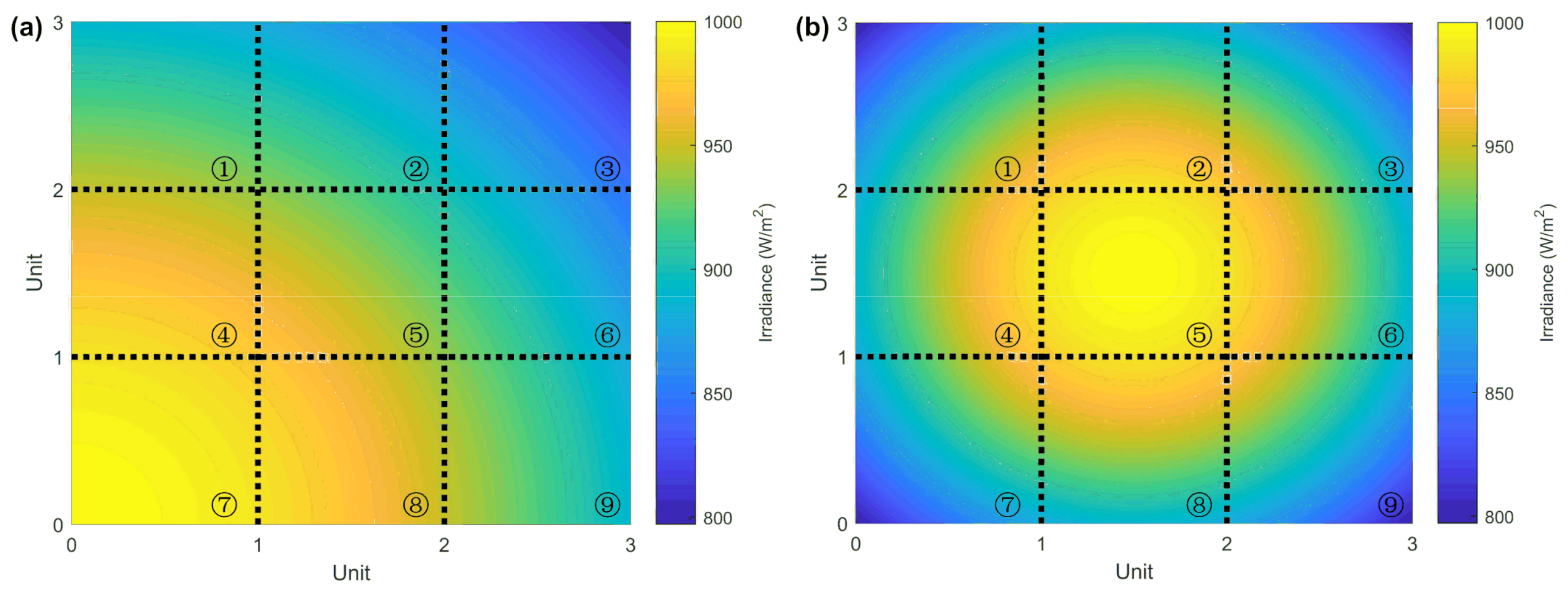
In the spatial-varying irradiance case, nine solar cells were divided into different regions in which the light irradiance radiated from one angle or center symmetrical, as is shown in
Figure 9a,b respectively. The irradiance distribution in
Figure 9a is denoted by corner irradiation, while that in
Figure 9b is denoted by middle irradiation. In both spatial distributions, maximal and minimal light irradiance were controlled to be 1000 W/m
2 and 800 W/m
2. The average light irradiance in both distributions was 925.5 W/m
2. The testing solar cell was denoted by the 10th solar cell, and was under constant light irradiance of 800 W/m
2. In the initial simulation step, i.e.,
t = 0, the 10th solar cell was connected with and measured by the voltage sensor to obtain its open-circuit voltage
V10,oc and MPP voltage
V10,mpp. In the PC method, the 10th solar cell was steadily connected with the voltage sensor. In the SPC method, the 10th solar cell was alternatively switched in and out with other solar cells, and MPP calculation took place only when it was switched out. The switching duty cycle was set as 1:10. In the proposed method, all ten solar cells were connected to the voltage sensor in the sequence of 10, 1, 2…, 9, repetitively, each exhibiting the duty cycle of 1:10.
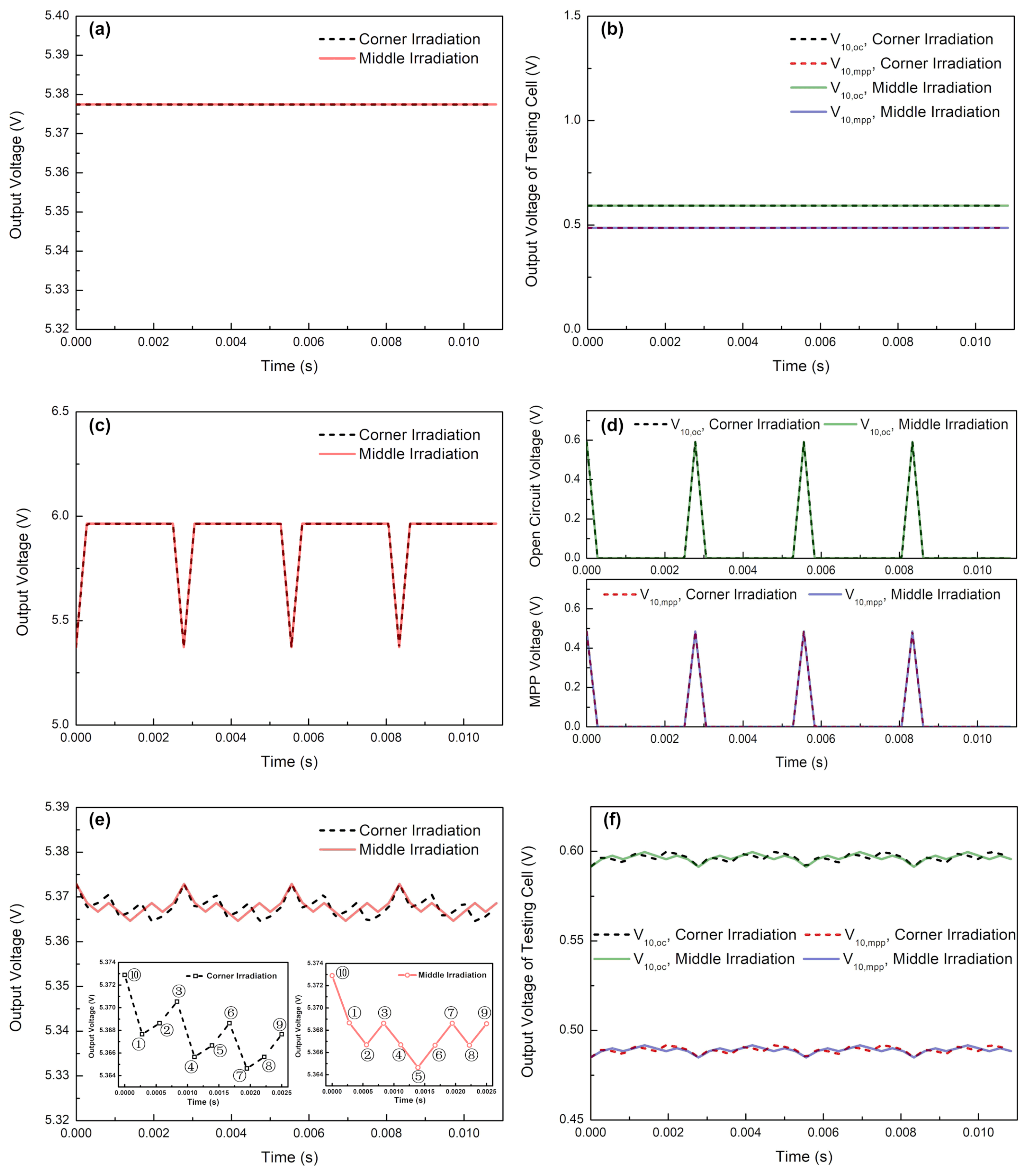
Figure 10 compares the output voltage of the proposed method with PC and SPC methods. For the PC method, as is shown in
Figure 10a, the output voltage of the system was generated by nine solar cells steadily, and thus output voltage curve was a flat line representing 5.38 V. Since the average light irradiance in both corner irradiation and middle irradiation was the same, the difference in the output voltage can be neglected.
Figure 10b shows the curve of
V10,oc and
V10,mpp for the tested 10th solar cell. As the 10th solar cell was under constant irradiance of 800 W/m
2, regardless of corner irradiation or middle irradiation, both
V10,oc and
V10,mpp were identical flat lines in two spatial-varying irradiance cases. For the SPC method,
Figure 10c shows the output voltage of all solar cells. Again due to the same average light irradiance, output voltage curves were the same for corner and middle irradiation. Still, output voltage curves fluctuated between 5.96 V and 5.37 V, corresponding to ten and nine solar cells switched in. In
Figure 10d, the voltage curves
V10,oc and
V10,mpp of the SPC method were characterized by a series of spikes, which were in synchronization with the measurement window phase of the 10th solar cell. Still, both
V10,oc and
V10,mpp values of the chosen semi pilot cell were constant, which cannot reflect the spatial distribution differences.
Figure 10e,f shows the results of the proposed method. It can be seen from
Figure 10e that, by consecutively changing the testing solar cell, different spatial distributions of irradiance can be traced, as output voltage curves of corner irradiation and middle irradiation are different. The two insets in
Figure 10e show the detailed changing process of output voltage in corner irradiation and middle irradiation, with the numbers indicating the specific solar cell under measurement. The trend of the changing output voltage was in accordance with the light irradiance distribution shown in
Figure 9.
Figure 10f shows the
V10,oc and
V10,mpp curves of the proposed method. For corner irradiation and middle irradiation, the voltage curves in the two cases were no longer identical, proving the effectiveness of the proposed method in tracing spatially variant irradiance. Since
V10,mpp is changing with each solar cell, all solar cells in the photovoltaic system can be set at its MPP. In this way, the optimization of output power can be achieved at an arbitrary location, which is suitable to be combined with distributed sensing and applied in smart photovoltaic systems.
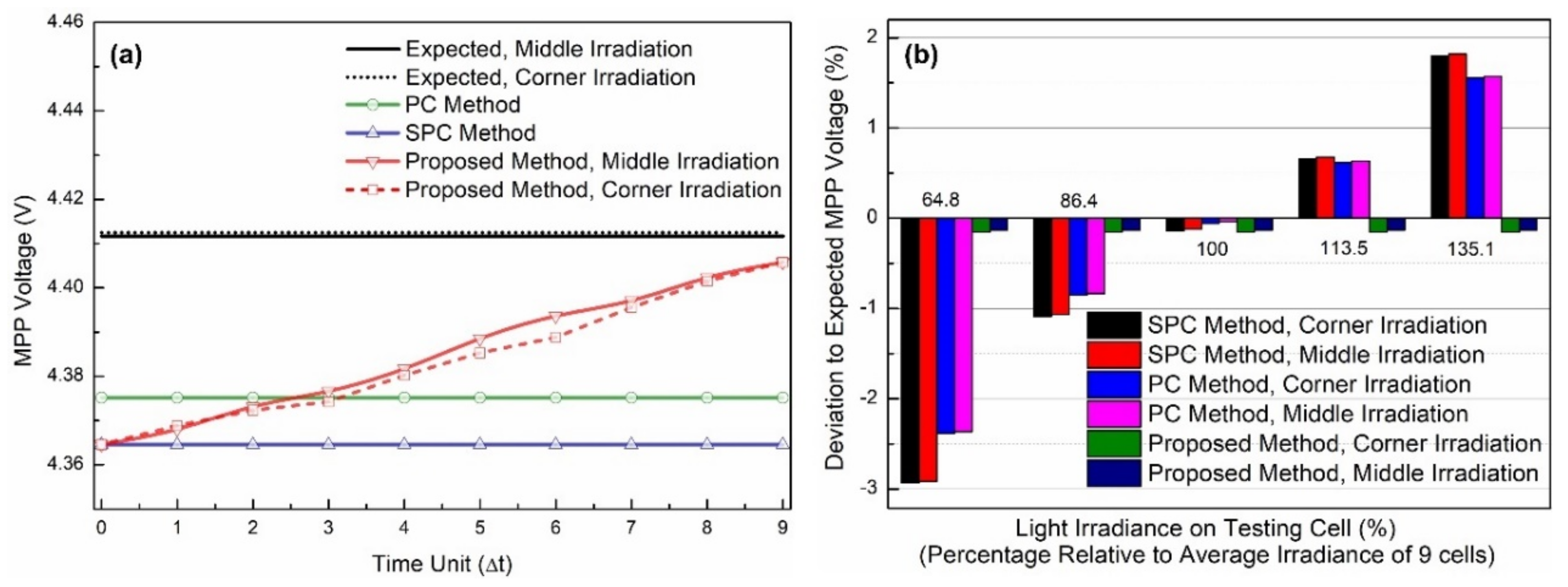
For PC, SPC and the proposed method,
Figure 11 compares the obtained MPP voltage with expected MPP voltage in corner irradiation and middle irradiation. The expected MPP voltage is simulated for the nine solar cells with irradiance distributions shown in
Figure 9, via sampling output voltage and current under different loads. For both corner and middle irradiation, the expected MPP voltage is 4.413 V. In
Figure 11a, the time unit Δ
t represents the measurement window. For PC and SPC method, since the chosen cells are under constant irradiance in both spatial distributions, the chosen cells reflect the constant MPP voltage of 4.375 V and 4.365 V after nine time units, respectively. However, for the proposed method, because each solar cell is consecutively measured, the MPP voltage value is continuously updating. After nine time units, all solar cells have been traversed, and the updated MPP voltages of 4.406 V in both distributions are much closer to the expected MPP voltages, demonstrating higher accuracy of 99.85% compared with the PC method (99.15%) and SPC method (98.92%).
Figure 11b further points out that the deviation to expected MPP voltage is relevant to light irradiance on the testing cell, which is expressed as a percentage to average irradiance on nine solar cells. It can be seen that, for PC and SPC methods, the deviation increases as the percentage increases or decreases. Only when light irradiance on the testing cell equals average irradiance, the deviation can be controlled below 0.14%. When the percentage reduces to 64.8% or increases to 135.1%, the deviation can be up to −2.93% and 1.81%, respectively. While for the proposed method, the deviation is controlled to be less than 0.15% regardless of the testing cell irradiance percentage, which again proves the effectiveness of the proposed method in situations with spatially varying irradiance.
5. Experiment
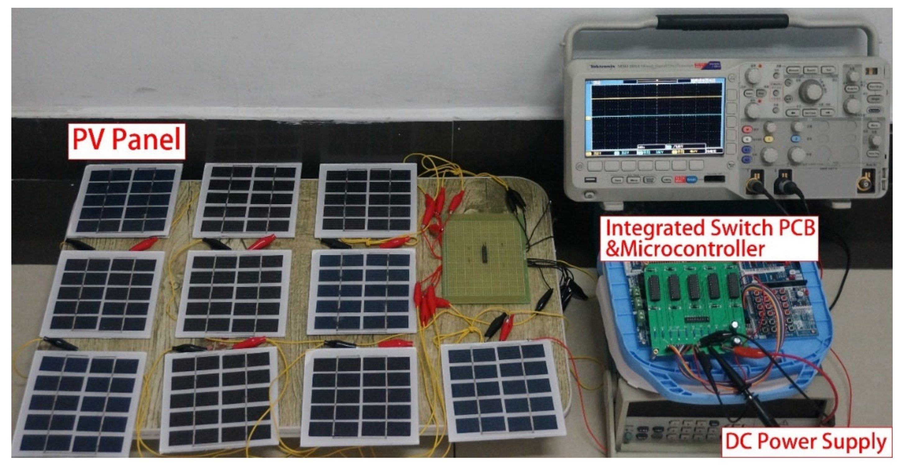
Experimental verification of the proposed on-site traversal FOCV method was conducted on the solar panel scale. The output characteristics of the ten solar panels (6 W) were: Voc = 7.2 ± 0.2 V, Isc = 1.1 ± 0.1 A. The ten pairs of SPDTs were realized by five integrated analog switch chips MAX394EPP, each with two pairs of SPDTs. The micro-controller STC90C516RD+ is selected as the controlled pulse generator. The pulse width was set to be 200 ms, i.e., the measurement time window for each solar panel was 200 ms, and one cycle of system operation was 2 s. The control strategy was based on the precision timing of the crystal oscillator, so that interrupt service routine was called every 200 ms to alter the voltage level of analog switch input. The ten pairs of SPDTs were thus switched on and off consecutively. The output voltage of nine solar panels in series
Vout was recorded on an oscilloscope.
Figure 12 shows the photo of the experimental system, including ten solar panels, SPDT switch circuitry integrated on printed circuit board, micro-controller and oscilloscope, as well as a DC power supply for powering analog switches and the micro-controller.
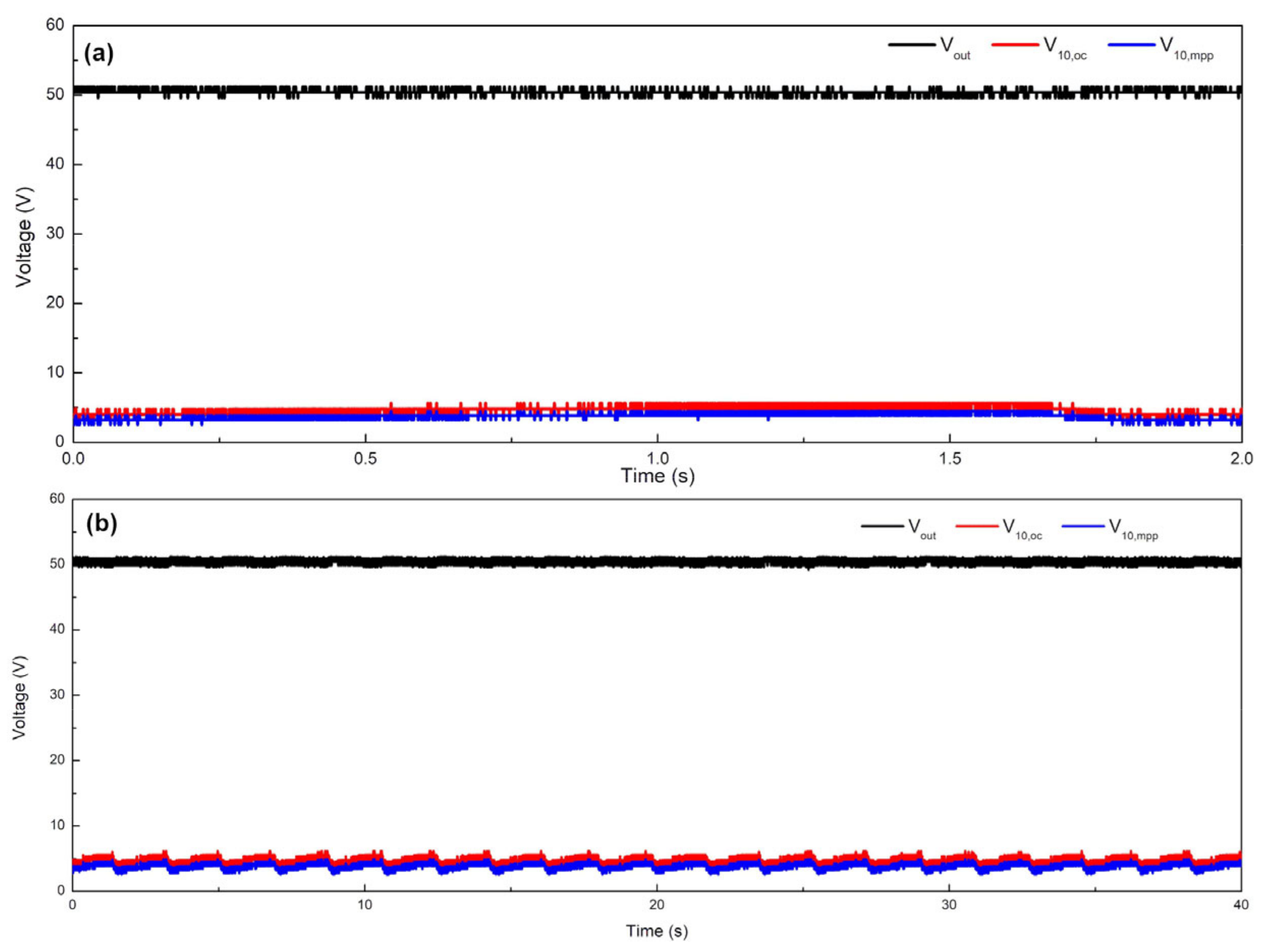
During the test, the light irradiance of the ten solar panels was controlled to be around 785 W/m
2.
Figure 13 shows the testing results under constant light irradiance. In
Figure 13a,
Vout reaches 50.4 V and its waveform is generally stable. During the 2 s system cycle, both
V10,oc and
V10,mpp experiencd slight changes due to non-uniform light irradiance distribution on all solar panels. The fluctuations of the
V10,oc and
V10,mpp curves also demonstrated that the diverse output performance of each solar panel can be effectively traced by the proposed method. The average value of
V10,oc was approximately 4.76 V, and the average value of
V10,mpp is 3.85 V. The output voltage curves in 20 system cycles have also been tested. As is shown in
Figure 13b, both
V10,oc and
V10,mpp exhibit clear periodicity, while V
out remains generally stable throughout 40 s. The periodicity of
V10,oc and
V10,mpp is in accordance with fluctuations within one system cycle. The ripple factor of V
out is 1.55%, which is mainly due to switch operations. The obtained MPP voltage can be further transferred to DC–DC converter to adjust load capacity to achieve maximum output power and to enhance conversion efficiency under real environmental conditions. Since the experimental fluctuations of
V10,oc and
V10,mpp curves reflect the non-uniform performance of all solar panels, it is expected that the proposed method is applicable both in constant irradiance and in time-varying or spatial-varying irradiance environment.
6. Discussion
The proposed method offers the possibility to combine with distributed sensing by locating and controlling specific solar cells or solar panels. As the size and cost of switching elements and control units on circuit boards are continuously decreasing, it is expected that the cost of the proposed method can be contained at a relatively low level. Integration and packaging technologies such as the Package-on-Package (PoP) will also help to reduce the cost for on-chip realization. The endurance of the electronic switches has been significantly improved over the years, so that the reliability of the system will be enhanced to match the lifetime of the solar cells or solar panels.
Despite the efficiency loss arising from the fact that the output voltage of one unit is not connected to the load for purpose of measurement, it is expected that the dual advantages of enhanced MPP accuracy and reduced ripple factor outweigh such efficiency loss. Moreover, for large scale photovoltaic systems with more than 100 units, the efficiency loss can be diluted to approximately 1%. In the distributed sensing configuration, the number of units can be even higher due to the exclusion of laying restrictions, which renders the efficiency loss negligible.
The installation complexity of the proposed method is relatively low. As can be seen from
Figure 6 and
Figure 7, all units are connected using the same schematic, so that required circuits take
The form of blocks of the unit circuit and the connection can be achieved by a plug-in through corresponding pins on the solar unit and the required circuits. The installation complexity can be further reduced if the unit circuit is integrated on-chip for solar cells or solar panels.
The chief advantage of the proposed method is the ability to measure FOCV and calculate MPP based on specific solar cells or solar panels, which offers the possibility of novel MPPT configuration through combination with distributed sensing. Based on this, future works can be carried out concerning remote control strategies, traverse conditions, and environmental limit conditions, etc. These future works will incorporate distributed sensing into optimizing MPP algorithms, which is conducive to enhancing efficiency and simplifying management for smart photovoltaic systems.


