Abstract
How to locate missing rods within a micro-structure composed of a grid-like, finite set of infinitely long circular cylindrical dielectric rods under the sub-wavelength condition is investigated. Sub-wavelength distances between adjacent rods and sub-wavelength rod diameters require super-resolution, beyond the Rayleigh criterion. Two different methods are proposed to achieve this: One builds upon the multiple scattering expansion method (MSM), and it enforces strong sparsity-prior information. The other is a data-driven method that combines convolutional neural networks (CNN) and recurrent neural networks (RNN), and it can be applied in effect with little knowledge of the wavefield interactions involved, in much contrast with the previous one. Comprehensive numerical simulations are proposed in terms of the missing rod number, shape, the frequency of observation, and the configuration of the tested structures. Both methods are shown to achieve suitable detection, yet under more or less stringent conditions as discussed.
1. Introduction
Micro-structures most of the time consist of a number of elements of the same nature, which are distributed in a periodic fashion within a certain region of space, and the characteristic size of such elements and their spacing usually are sub-wavelength—measured w.r.t. the wavelength of operation for the time-harmonic single-frequency electromagnetic signals assumed to be operated upon [1]. Such micro-structures may have a number of applications in industry and daily life, so a good understanding and analysis is necessary. Furthermore, they prove to be, in view of their high behavioral complexity, a good testbed for novel imaging procedures.
The micro-structure investigated in the present contribution is in accord with the above, and it is made of of a grid-like set of a finite number of infinitely-long (those would be long enough in experimental practice to neglect end effects) circular cylindrical dielectric rods, the radius of each rod being quite small and the adjacent rods being also quite close to one another, the diameter and spacing being less, even far less, than half a wavelength. Since the geometrical features of the micro-structure are sub-wavelength, the main challenge is how to achieve meaningful localization, resolution-enhanced, or better said, super-resolved, if some defects were to arise in the considered micro-structure.
Yet, super-resolution is hard to achieve by conventional methods with the geometrical features with which one is faced. This calls for smart approaches, while trying to mitigate computational costs and being reliable even if the data are erroneous or scarce. As a result, conventional methods need to be evolved for proper prior information to be accounted for, while data-driven methods can certainly provide some new paths of the solution, relying not on strong priors, in contrast, but extensive data computations beforehand
In any case, a good understanding of the physics as the support of the wavefield analysis remains a prerequisite, and the characterization of the material structures from electromagnetic fields scattered under given illuminations should be analyzed in a proper mathematical framework; so, herein, two methods are proposed to carry out the forward modeling of the micro-structure under investigation.
The closed-form multiple scattering expansion method (MSM) is specialized to the circular cylindrical rod case, involving standard cylindrical wave expansion of the fields tailored to circular boundaries, and it is quite accurate for the investigated structure due to the peculiar geometry of the rods; non-circular rods could however be treated, but far more intricate expansions should be devised (see [2] as a good example);this is left aside here in view of the subwavelength features and associated prototype(s) as well.
Another approach, more brute force yet applicable to any geometry of rods whether needed, is the well-known method of moments (MoM), which converts the integral equations that describe the field into a discrete system, choosing for simplicity MoM with pulse basis functions and delta testing functions thereafter.
Once having modeled the forward problem, the inverse one can, as hinted at in the above, be tackled by various methods from analytical ones to learning ones.
An analytical method based on sparsity information is proposed first, which takes sparsity as (strong) a priori and which relies on MSM in order to deal with the wavefield due to the interacting circular cylinders. Considering the system we are faced with, one can assume that missing rods are few compared with the rods effectively present, so those missing ones can be treated as a few non-zero contrast sources (to be determined during probing), located somewhere inside the periodic structure.
Examples of such an approach are found in [3] (this is about looking for a radiating source in a metal micro-structure since the MSM easily stands for perfectly electrically conducting rods) and in [4] and, for the most elaborate analysis in that framework, ref. [5] (those last two contributions apply to variously damaged planarly-layered fiber-based laminates). One should also, without pretense to exhaustivity in a fast evolving field, refer to [6] with specific zero-order simplifications within the MSM during the fault detection of a diffraction grating and in a linearized setting of the inversion (tailored to band-gap photonic crystals now) to [7]; there exist similar developments in elasticity, pioneered in particular in [8], but their full coverage is beyond the scope of this brief tour of the literature especially as they involve intricate elasticity issues that tend to differ much from the electromagnetic ones.
As for an initial work by the authors using MSM and a sparsity constraint compared with standard time reversal, whose behavior is readily explained by first-order homogenization of the micro-structure whenever contrasts are low enough, the reader being referred to [9].
Now, in great contrast with the above, one can focus on deep neural networks since those are known to play an important role among numerous learning methods during this era of big data, the increase of the number of layers sharply improving the performances. That is, unlike analytical methods for which the problem is explicitly defined and domain knowledge carefully engineered in the solution, as insisted upon in the above, learning methods do not benefit from prior knowledge, or, better said, do not require it, and instead, they make use of large datasets to learn the unknown solution to the inverse problem.
Quite many contributions have already been made by researchers in the imaging field, with different architectures proposed for different situations [10,11]. Convolutional neural networks (CNN) and recurrent neural networks (RNN) are two of the most important deep learning models, and they are widely used in tasks like natural language processing, image processing, and pattern recognition, to mention but a few fields of application.
CNN is a type of artificial deep learning neural network designed to analyze visual images, while RNN is designed to process sequential data and recognize patterns, which have achieved good results in text generation, machine translation, and face detection [12,13]. As for electromagnetics, many use CNN to deal with the inverse scattering problem [14,15,16]. RNN is also applied in magnetic resonance image reconstruction [17], while there exist works on the equivalence between wave dynamics and recurrent neural networks [18].
The mapping from the collected field data to the information of the region of interest (ROI) by CNN is also dealt with by the present authors as described in a previous contributions [19] and, later on, [20]. Notice that, compared with using the images of the ROI as the output, as was illustrated in those two, the index of rods as the output contains less information (from the former, the size and shape of rods and distance between rods can be interpreted).
The main focus of the present contribution is to confirm first that a sparsity-constrained inversion can be built effectively and provide a proper diagnosis of missing rods, yet that it pales in comparison in many aspects with respect to a novel combination of two known tools of the deep learning community, as convolutional neural networks and recurrent neural networks, pending the computational cost of dealing with large amounts of data to get the most versatile solver.
The work is organized as follows. In this section, we introduced the issues at stake and quickly toured the literature. In Section 2, the problem is modeled and the solutions sketched. In Section 3, the sparsity-constrained inversion is described, with proper use of previous references, and numerical simulations illustrate the performances. In Section 4, the RNN and CNN are designed to end up with the combined CRNN approach, with various numerical simulations as well. A brief recapitulation and an outline of on-going investigations and of the developments envisaged are in Section 5.
2. Modeling of the Problem
2.1. The Micro-Structure under Investigation
An illustration of the dielectric micro-structure as considered in a laboratory-controlled experiment carried out in a microwave anechoic chamber is proposed in Figure 1 (left); refer to [20] where a prototype involving metal rods, not polymeric ones now, was introduced first and antennas inside, not outside, being described earlier in [3].
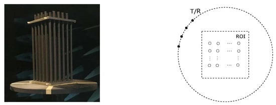
Figure 1.
Illustration of the experiment in an anechoic chamber (left) and 2D modeling (right).
The corresponding model involves a finite number of circular cylindrical rods in a given region of interest (ROI). Those are assumed of infinite length in the vertical direction, and the 2D cross-section of the micro-structure considered is sketched in Figure 1, right. The rods are indexed from one to L, from left to right, top to bottom in the figure, where L is their total number if a sound micro-structure (in effect, one considers rows and columns, L even, but other distributions could be considered as well). Rods are homogeneous, linear, and isotropic, their common relative dielectric permittivity being denoted as , their relative permeability being the unit, ; some of them may be absent, or equivalently, this means that they exhibit a relative permittivity . Each rod (if present obviously) is of the same radius R, and the center-to-center distance between adjacent rods is d, all those quantities being a fraction of the wavelength at the operation frequency (radii one-tenth of a wavelength or less and spacings at most half a wavelength will be considered). Several transverse-magnetic (TM) polarized transmitters and receivers are put outside the ROI on the same circular line S, at a subwavelength distance from the micro-structure center.
2.2. Method of Moments
The electromagnetic interaction between the wave and material object is described by the Helmholtz wave equation. Applying Green’s theorem to it and taking into account the classical conditions of the continuity of the fields and of radiation at infinity, this problem can be appraised from an integral representation of the TM electric field (with a single vertical component) consisting of two coupled integral equations, observation and state equations. The solution requires their discrete counterparts, which are obtained in an algebraic framework using the method of moments [21]. The state equation describes the electrical field when the transmitter emits,
where is the total scalar-valued electric field, the incident one, k the wave number in air, and the 2D scalar Green’s function, being the dielectric contrast defined as , and D represents the ROI. Correspondingly, the observation equation is written as:
where is the scattered field and S represents the observation region. is the contrast source, and two operators and are defined as:
so and can be calculated as:
To tackle the above numerically, the ROI is divided into M small cells, as depicted in Figure 2, within which the electric field and dielectric permittivity are assumed to be constant. The method of moments in effect transfers the integral equation into a linear system as is well-known, here pulse basis functions and delta testing functions being used for simplicity. Let us emphasize that the MoM works for any shape of rod, so the hypothesis of circular rods is not a restriction to it.
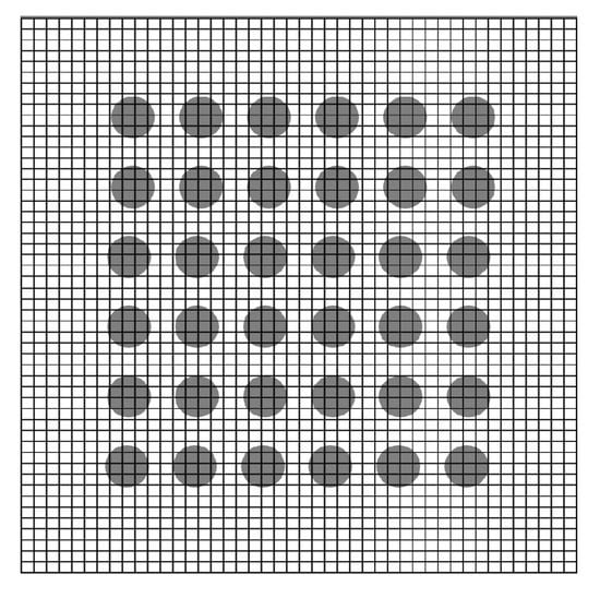
Figure 2.
ROI divided into M × M cells.
2.3. Multiple Scattering Expansion Method
The direct problem can be modeled from the physics of the interaction between a known interrogating wave and a known object. The multiple scattering expansion method is the mathematical formalism used to describe the propagation of a wave through a collection of scatterers and is already thoroughly applied in acoustics and optics, e.g., [22], and many others, e.g., [4,5,7] and a number of references quoted in those. In the research, line sources are used to illuminate the structure; sources are of unit amplitude and radiate a field , with zeroth-order first-kind Hankel function and the distance between the observation point and line source. For the completeness and self-consistency of the contribution, we go into the formulation in some detail now.
In the vicinity of the l-th rod, the exterior electric field in local coordinates is written as:
where and are the first-kind Bessel function of m-th order and the Hankel function of m-th order, k is the wave number in air, and are the coordinates of the observation point within the local coordinate system originated at the center of this l-th rod.
The field outside a given rod then is the sum of fields scattered by all rods and the emitting source,
where L is the number of rods as already introduced, the location of l-th rod, and the location of the source. Applying Graf’s addition theorem to Equation (7) and expressing the global field expansion into the local coordinates of the l-th cylinder, one arrives at:
where:
so the matrix form is
where (, ) are the local polar coordinates of , meaning the position of cylinder j vs. cylinder l, and are the local polar coordinates of . The interior field expansion within rod l in such a local system is:
where is one if a line source is present and zero otherwise, are the polar coordinates of the line source in the local coordinate system associated with the l-th rod. The boundary continuity conditions sketched in Figure 3 are expressed in terms of cylindrical harmonic reflection and transmission coefficients:
in matrix form,
and the expression of is:
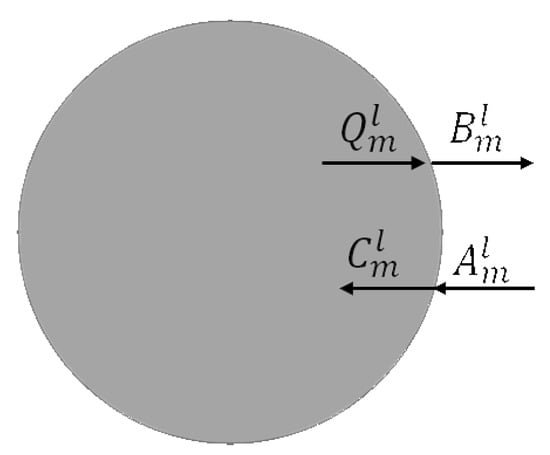
Figure 3.
Cylindrical wave expansion coefficients; see the text.
To calculate the aforementioned reflection and transmission coefficients, the boundary conditions of the TM field, within the cylindrical coordinate system, are enforced, and , , , and follow. The field computed accordingly is easily applied in the sparsity-constrained inversion; see Section 3.
2.4. Comparison of the Two Modeling Methods
To quickly illustrate the reliability of the two approaches in the present case, MSM and MoM, comparisons are proposed in Figure 4, with or without missing rods. The parameters of the micro-structure for this comparison are dielectric contrast , , , at a 3 GHz operation frequency. There are 36 rods when the micro-structure is sound, reduced to 33 when damaged (missing ones in the example are numbered 2, 12, and 30, but this would work for any other arrangement). A single source is set at location (0.72, 0), and thirty-six receivers that are equally-spaced on the circular line of observation at (0.72 from the center) collect the scattered fields.
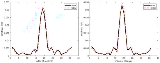
Figure 4.
Comparison of the two modeling methods for a contrast of 2.5 with three missing rods (left), numbered 2, 12, and 30 (not shown), and no missing ones (right). MSM, multiple scattering expansion.
Not only for the case shown here when the dielectric contrast is equal to , but in effect as observed up to such a contrast reaching of the order of 10, the scattered fields calculated by MSM and MoM match; though there still exists a difference at some receivers, which might be caused by the discrimination of MoM, i.e., the number of cells used in it, herein the region of interest in divided into cells, and/or the truncation of the cylinder wave expansion (the upper mode number being automatically chosen, Reference [5] and a number of previous references quoted therein) within the MSM.
3. The Sparsity-Constrained Inversion
The proposed method is based on direct modeling by means of the multiple scattering expansion, which is handy as one can model complicated interacting wavefields in a fast and accurate way. Imaging performances are expected to be good since much prior information is provided as well. The sparsity-constrained method is built so as to get the index solution from the collected fields. The number of missing rods is just a few compared with the one of the normal rods. In the problem we are faced with, missing rods can be treated as equivalent sources of unknown location. Equivalence theory then provides a link between collected data and expansion coefficients of such equivalent sources, any non-zero element indicating the index of a missing rod.
3.1. A Sketch of the Method of Operation
The starting point of the analysis is the Lippmann–Schwinger integral formulation:
where E denotes the single-component total electric field due to the well-organized sound micro-structure, and quantities with ∼above are associated with the disorganized structure that exhibits missing rods. is the cross-sectional area of the l-th missing rod, and is Green’s function for the case that the line source is located at when there are no missing rods. One has:
and:
where are the polar coordinates of in the local coordinate system w.r.t. the l-th missing rod. Substituting Equations (17) and (18) into Equation (16), is calculated by Equation (15). Therefore,
where if the l-th rod is missing, parameter is non-zero, and is zero otherwise, indicates the parameter corresponding to the l-th rod and m-th mode and the j-th rod and n-th mode. We remind that a more theoretical background and a pioneering use in the photonic crystal realm were given in [7]. Refer to [4,5] for non-destructive testing of planar fiber laminates.
Comparison of in Equation (19) with Green’s function in Equation (17) shows that the calculation of the former can be performed as that of the latter, save changing to . As are coefficients of the field due to an interior line source, can be interpreted as those due to a cylindrical source.
Considering for generality a receiver array with elements and a source array with elements, for the -th source, the values of collected by the receiver array are made of a column vector with dimension , the position of the n-th receiver element, subscript T marking the transpose, so , being the coefficient vector associated with the l-th rod, and . With a low-frequency incident field, provided that the radius of the rod , can be smaller than one, so M = int is reduced to zero without a security factor. As the expression is invariant with the sources, taking different as columns, the data matrix Y is defined as , and denoting ,
Letting and adding Gaussian noise from geometry uncertainty and material parameters, the problem is summarized as:
From the multi-static response matrix, getting the indexes of the missing rods is ill-posed. If the l-th rod is missing, the corresponding element in is non-zero. If only a few rods are missing, most elements in are null, and is sparse; sparsity can be evaluated via an norm counting the number of non-zero elements. The optimal problem can be stated as:
where the parameter is decided by the noise variance.
Exhaustive enumeration of all possible locations of non-zero entries in , which is NP hard, is required for the norm. Another way to appreciate the sparsity works when there are enough collected data, as the norm provides good approximation of the norm, being:
in which based on numerical trials, so the optimization is rewritten as:
and can be tackled by applying the gradient descent method on the Lagrangian form,
where parameter realizes a trade-off between the sparsity and quality of data fit. If increases, more weight is on the sparsity. Using gradient descent to update and select the parameter by the L-curve methods, one can solve the optimization problem with which we are faced. When ,
so for each update,
where and ; should be small enough to not affect the solution behavior.
3.2. Results of the Sparsity-Constrained Method
The performance of the sparsity-constrained method for different missing rod numbers is studied first: missing one rod, two rods, and three rods; see Figure 5. The SNR is equal to 30 dB, and the rod contrast is equal to 2.5. All geometrical features are as in the modeling considered before, save that 36 sources are considered at the same locations as the 36 receivers. As shown, the identification of the missing rod index is reached.
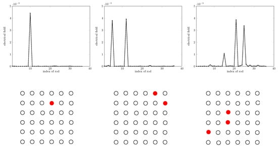
Figure 5.
Retrieval for 1, 2, and 3 missing rods, left to right, and sketches of the micro-structure. MSM, multiple scattering expansion.
In the same setting unless otherwise specified, tests for different values of d and of R were carried out in order to further validate the robustness of the method. Figure 6 displays the result in the case of different radii of the rods. Figure 7 displays this for different distances between rods. It turns out that the proposed method works suitably.
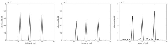
Figure 6.
Retrieval for different radii, from left to right, . Spacing d is kept at . Missing rods (not shown) are of indexes 12, 20, and 30.
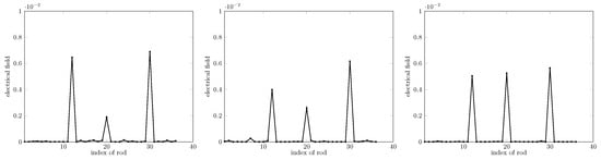
Figure 7.
Retrieval for different spacings d, from left to right, . The rods’ radius R remains . Missing rods (not shown) are of indexes 12, 20, and 30.
Again, in the same setting unless otherwise specified, the cases of different contrast values are considered. As shown in Figure 8, obviously, when the contrast of a rod is as high as 7.5, the sparsity-constrained method does not succeed in locating a missing one. Much testing carried out pinpointed that the highest value of contrast yielding reliable results is about seven, too high a contrast, thus being a limitation of the proposed method.
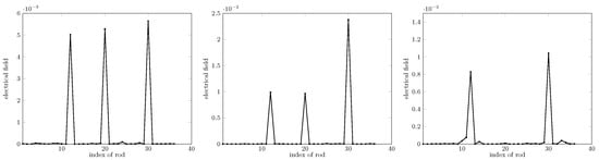
Figure 8.
Retrieval for different dielectric contrast values, from left to right. Contrasts are 2.5, 5, and 7.5, respectively. Missing rods (not shown) are of indexes 12, 20, and 30.
4. CRNN Learning Method Based on Combining CNN and RNN
The main question is now to see whether or not one can leave aside most priors and deploy as indicated in the Introduction a proper blend of convolutional neural networks (CNN) and recurrent neural networks (RNN) to achieve super-resolution imaging of the micro-structure when damaged, most of the computational burden being with the construction of the field data base and not with the solution of the inverse problem with which we are faced.
4.1. Main Principles
Without going back to the abundant literature that we presented in the Introduction, CNN is known to have strong local modeling capabilities and can extract the features of interest. RNN is recurrent in nature as it performs the same function for every input of data while the output of the current input depends on the past computation. Therefore, the proposed approach combines CNN and RNN to take advantage of both of them. CNN processes the initial collected field and recognizes the features, and RNN uses the known features to make sense of the field and put together a cohesive description, the reconstruction information being shared across the multiple iterations of said process. Figure 9 sketches the proposed frame, denoted from now on as CRNN (C meaning combined).
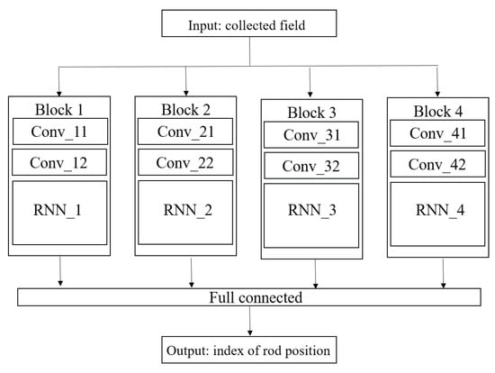
Figure 9.
Architecture of the proposed combined RNN (CRNN) structure.
4.2. CRNN Probing of The Micro-Structure
Let us consider the already investigated micro-structure to emphasize the main attributes of CRNN. As shown, the input of the structure is the field collected by the 36 receivers when the ROI is illuminated by 36 transmitters at the same distance 0.72, and the distance between rods d is equal to , while the radius of the rod is equal to (at 3 GHz); thus, the size of the input is . Meanwhile, the output is the index of the rods, i.e., a list of data containing only two values, for example , the size of which is the number of rods, wherein represents a normal (present) rod and one represents a missing rod. Three-thousand examples in total are used to train the network here. One example of the dataset is given in Figure 10, the real part of the collected field being the input of the network and the index of the rod being its output.
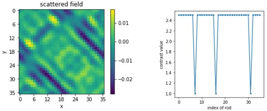
Figure 10.
Example of the dataset.
In this structure, four parallel blocks compose the main body, each block containing two convolutional components and one recurrent neural network layer; in each convolutional component, one convolutional layer with batch normalization and the ReLU function is applied to achieve feature extraction. The convolutional layer with a well-chosen kernel size in each block has the ability to extract local features. ReLU, a non-saturated function, is chosen as the activation function, and applying it to the output of a linear transformation can produce a non-linear transformation. Batch normalization normalizes the input and hidden layers by scaling the activations to alleviate the internal covariate shift [23].
The details of the RNN layer are shown in Figure 11, each RNN layer having 64 cells with the same structure. The input of the RNN is made of the extracted features coming from the convolutional components, and the output is combined with another three outputs from another three blocks. After a linear transform, the output of the structure is the corresponding index of the rod position.
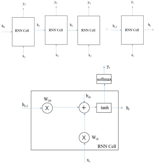
Figure 11.
Details of the RNN layer and the RNN cell.
As for the choice of the RNN cell, two types have been considered: the simple RNN and the gated recurrent units (GRUs) [24]. The detail of the simple RNN is shown at the bottom of Figure 11; the t-th cell receives both and the state from the last cell , then produces the for the next cell. The GRU enjoys some changes w.r.t. simple RNN, both being shown to have similar performance however.
The loss function that we henceforth use is:
in which N is the number of samples at each iteration. For the i-th sample, and are the prediction value generated from the RNN and the ground truth, respectively.
The learning algorithm chosen is the Adam algorithm [25] (sketched for completeness in Appendix A), which is an adaptive learning rate optimization algorithm, an algorithm for first-order gradient-based optimization of stochastic objective functions, based on adaptive estimates of lower order moments. It derives from the optimization methods AdaGrad [26] and RMSProp [27]. It leverages the power of adaptive learning rate methods to find individual learning rates for each parameter. The Adam algorithm has been designed to combine the advantages of AdaGrad, which works well with sparse gradients, and of RMSProp, which works well in on-line and non-stationary settings.
Coding is realized in its entirety on the Pytorch platform. Figure 12 shows the iteration curve during training. The GPU NVIDIA Quadro M620 was used, which took about 35 min to perform a training.
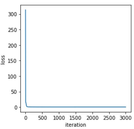
Figure 12.
Iteration curve during the training.
4.3. Results of CRNN
Different tests from the configuration of the micro-structure, including the rod shape, to the method of observation, including the frequency and number of observations, were preformed in order to validate the performance of the proposed network.
Three-thousand datasets collected at 3 GHz by the application of the MoM were used to train the network, and one-hundred examples (again with MoM), which were not included in the training set, were used to test the performance of the designed network.
In Figure 13, three different examples are displayed: 1 missing rod, 2 missing rods, and 3 missing rods. The error is 0.0029, where it is defined as the mean squared error. For 1 GHz, with the same configuration as for 3 GHz, the error reaches 0.0036, instead of 0.0029 when the frequency is 3 GHz, yet CRNN still achieves the correct localization of missing rods (notice that all distances are absolute, the 3 GHz frequency being chosen as the nominal one).
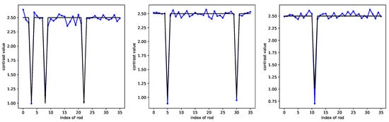
Figure 13.
CRNN retrieval at the 3 GHz operation frequency, from left to right: 1, 2, and 3 missing rods (the black line represents the ground truth, the blue line the CRNN results).
To be in better accord with the experiments under way, we only took the data for which one single transmitter radiates from 36 positions all around the micro-structure and for which there is only a single receiver that can collect the scattered field, directly faced by the transmitter (180 ). As a result, in this forward-scattering configuration, the number of collected field data is quite reduced, from to for each sample. As one can see in Figure 14, there are larger fluctuations, and the error is increased; yet, the index of missing rods can still be recognized.

Figure 14.
CRNN retrieval with fewer data (the black line represents the ground truth, the blue line the CRNN results).
To illustrate the potential influence of the shape of the rods, another training set for rods with a square shape was used to check the performance, the side of the square being equated to and the rods being spaced by . In Figure 15, the identification of the missing rod index performs well.
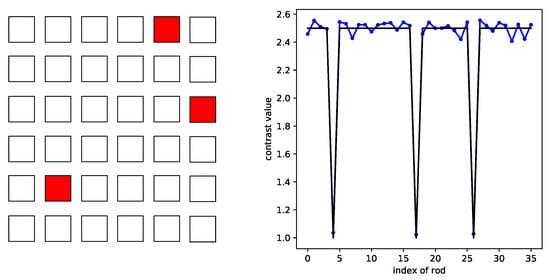
Figure 15.
CRNN retrieval for the square shaped rod distribution (the black line represents the ground truth, the blue line the CRNN results).
For now, the maximum missing rod number was limited to three, and to extend the validation, a complementary analysis where the maximum number of missing rods was five was run. The condition was the same as before: 3000 examples as the training set, another 100 examples as the test set. The localization results for different numbers of missing rods are shown in Figure 16, which are still acceptable.
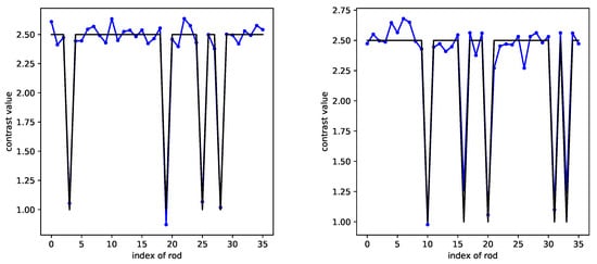
Figure 16.
CRNN retrieval for four (left) and five (right) missing rods (the black line represents the ground truth, the blue line the CRNN results).
5. Conclusions
In this contribution, two different methods have been proposed to realize the identification of the missing rod index within a dielectric micro-structure for different practical situations.
The sparsity-constrained method highly depends on a good understanding of the physics behind the scene, and the result is quite accurate and the calculation fast for each sample with different sizes of rods and distances between rods. Compared with the CRNN method, there is no need for a large number of data for training. However, it is strictly tailored to circular cylindrical rods, and the attached coordinate system, i.e., if the shape of the rods were to change, a new analysis should be run, while as seen from the CRNN results, the learning method still achieves good detection for square shaped rods.
The combination of RNN and CNN can indeed take advantage of both of them: CNN extracts the information from the initial field input; RNN uses the recurrent cell to avail itself of the inner linkage between fields. The potential of RNN then should be emphasized. Compared with using images of the ROI as the output [19,20], the index of rods as the output contains little information, since from the former, the size and shape of the rods and the distance between rods can be interpreted easily. In forthcoming works, RNN will be used to process time-sequenced fields, computed by FDTD or measured when pulses (synthetically generated from wideband time-harmonic illuminations) impinge on the structure.
In a rather different perspective, yet well aside this contribution, it would also be interesting to move onto Bayesian inference methodologies as seen in [28], about the inversion of conductors, wherein a binary enforcement mechanism (a pixel is either air or a reflector) is developed in a probabilistic framework.
The two approaches as proposed should not be limited to 2D geometries; the extension to 3D ones can be considered, though more complicated, whereas the application to controlled-laboratory data as mentioned is mandatory. A hybrid method combining the analytical method and the learning one could benefit from the physical background and contribute to the learning procedure from different aspects, which signals a new path [29,30].
Yet, the acquisition of enough useful data and the proper design and combination of methods are still facing difficulty. In some contrast, since in the experiment, the positions and other characteristics of the rods and antennas may be uncertain, this will also help to better appreciate the effect of data errors on the retrievals, beyond the standard Gaussian noise hypothesis.
Author Contributions
The work herein was completed as part of the Ph.D. investigation of P.R., advised by D.L. and M.S. All authors read and agreed to the published version of the manuscript.
Funding
No specific funding save the one provided by CNRS, CentraleSupélec, and University Paris-Saclay as the parent entities of the laboratory and employers benefited this investigation. P.R. is otherwise individually funded by the Chinese Scholarship Council.
Conflicts of Interest
The authors declare no conflict of interest.
Appendix A. Sketch of the Adam Optimization Algorithm, and Suppress All Else
| Algorithm A1: Sketch of the Adam Optimization Algorithm. |
|
References
- Ammari, H.; Zhang, H. A mathematical theory of super-resolution by using a system of sub-wavelength Helmholtz resonators. Commun. Math. Phys. 2015, 337, 379–428. [Google Scholar] [CrossRef]
- Maystre, D. Electromagnetic scattering by a set of objects: An integral method based on scattering operator. Prog. Electromagn. Res. 2006, 57, 55–84. [Google Scholar] [CrossRef][Green Version]
- Tu, H.; Serhir, M.; Ran, P.; Lesselier, D. On the modeling and diagnosis of a micro-structured wire antenna system. In Proceedings of the 2018 International Conference on Microwave and Millimeter Wave Technology (ICMMT), Chengdu, China, 7–11 May 2018; p. 8563875. [Google Scholar] [CrossRef]
- Liu, Z.; Lesselier, D.; Zhong, Y. Electromagnetic imaging of damages in fibered layered laminates via equivalence theory. IEEE Trans. Comput. Imaging 2018, 4, 219–227. [Google Scholar] [CrossRef]
- Liu, Z.; Li, C.; Zhong, Y.; Lesselier, D. Electromagnetic modeling of damaged fiber-reinforced laminates. J. Comput. Phys. 2020, 409, 109318. [Google Scholar] [CrossRef]
- Brancaccio, A.; Solimene, R. Fault detection in dielectric grid scatterers. Opt. Express 2015, 23, 8200–8215. [Google Scholar] [CrossRef] [PubMed]
- Groby, J.P.; Lesselier, D. Localization and characterization of simple defects in finite-sized photonic crystals. J. Opt. Soc. Am. A 2008, 25, 146–152. [Google Scholar] [CrossRef] [PubMed]
- Groby, J.P.; Wirgin, A.; De Ryck, L.; Lauriks, W.; Gilbert, R.; Xu, Y. Acoustic response of a rigid-frame porous medium plate with a periodic set of inclusions. J. Acoust. Soc. Am. 2009, 126, 685–693. [Google Scholar] [CrossRef]
- Ran, P.; Liu, Z.; Lesselier, D.; Serhir, M. Diagnostic within a dielectric micro-structure: Time-reversal and sparsity-constrained imaging. In Proceedings of the 13th European Conference on Antennas and Propagation (EUCAP), Krakow, Poland, 31 March–5 April 2019; p. 8740223. [Google Scholar]
- Lucas, A.; Iliadis, M.; Molina, R.; Katsaggelos, A.K. Using deep neural networks for inverse problems in imaging: Beyond analytical methods. IEEE Signal Process. Mag. 2018, 35, 20–36. [Google Scholar] [CrossRef]
- Massa, A.; Marcantonio, D.; Chen, X.; Li, M.; Salucci, M. DNNs as applied to electromagnetics, antennas, and propagation—A review. IEEE Antennas Wirel. Propag. Lett. 2019, 18, 2225–2229. [Google Scholar] [CrossRef]
- Cho, K.; van Merrienboer, B.; Gulcehre, C.; Bahdanau, D.; Bougares, F.; Schwenk, H.; Bengio, Y. Learning phrase representations using RNN encoder-decoder for statistical machine translation. arXiv 2014, arXiv:1406.1078v3. [Google Scholar]
- Mikolov, T.; Kombrink, S.; Burget, L.; Černocký, J.; Khudanpur, S. Extensions of recurrent neural network language model. In Proceedings of the 2011 IEEE International Conference on Acoustics, Speech and Signal Processing (ICASSP), Prague, Czech Republic, 22–27 May 2011; pp. 5528–5531. [Google Scholar] [CrossRef]
- Wei, Z.; Chen, X. Deep-learning schemes for full-wave nonlinear inverse scattering problems. IEEE Trans. Geosci. Remote. Sens. 2019, 57, 1849–1860. [Google Scholar] [CrossRef]
- Cui, L.; Zhang, Y.; Zhang, R.; Liu, Q.H. A modified efficient KNN method for antenna optimization and design. IEEE Trans. Antennas Propag. 2020, 68, 6856–6866. [Google Scholar] [CrossRef]
- Zhang, R.; Sun, Q.; Zhang, X.; Cui, L.; Wu, Z.; Chen, K.; Wang, D.; Liu, Q.H. Imaging hydraulic fractures under energized steel casing by convolutional neural networks. IEEE Trans. Geosci. Remote. Sens. 2020, 1–9. [Google Scholar] [CrossRef]
- Qin, C.; Schlemper, J.; Caballero, J.; Price, A.N.; Hajnal, J.V.; Rueckert, D. Convolutional recurrent neural networks for dynamic MR image reconstruction. IEEE Trans. Med Imaging 2019, 38, 280–290. [Google Scholar] [CrossRef] [PubMed]
- Hughes, T.W.; Williamson, I.A.D.; Minkov, M.; Fan, S. Wave physics as an analog recurrent neural network. arXiv 2019, arXiv:1904.12831. [Google Scholar] [CrossRef] [PubMed]
- Ran, P.; Qin, Y.; Lesselier, D. Electromagnetic imaging of a dielectric micro-structure via convolutional neural networks. In Proceedings of the 27th European Signal Processing Conference (EUSIPCO), A Coruna, Spain, 2–6 September 2019; p. 8903073. [Google Scholar] [CrossRef]
- Ran, P.; Qin, Y.; Lesselier, D.; Serhir, M. Subwavelength micro-structure probing by binary-specialized methods: Contrast source and convolutional neural networks. IEEE Trans. Antennas Propag. 2020, 1. [Google Scholar] [CrossRef]
- Jones, D.S. Field computation by moment methods. Comput. J. 1969, 12, 37. [Google Scholar] [CrossRef]
- Botten, L.C.; Nicorovici, N.A.P.; Asatryan, A.A.; McPhedran, R.C.; de Sterke, C.M.; Robinson, P.A. Formulation for electromagnetic scattering and propagation through grating stacks of metallic and dielectric cylinders for photonic crystal calculations. Part I. Method. J. Opt. Soc. Am. A 2000, 17, 2165–2176. [Google Scholar] [CrossRef]
- Ioffe, S.; Szegedy, C. Batch normalization: Accelerating deep network training by reducing internal covariate shift. arXiv 2015, arXiv:1502.03167. [Google Scholar]
- Chung, J.; Gulcehre, C.; Cho, K.; Bengio, Y. Empirical evaluation of gated recurrent neural networks on sequence modeling. arXiv 2014, arXiv:1412.3555. [Google Scholar]
- Kingma, D.P.; Ba, J. Adam: A method for stochastic optimization. arXiv 2014, arXiv:1412.6980. [Google Scholar]
- Duchi, J.; Hazan, E.; Singer, Y. Adaptive subgradient methods for online learning and stochastic optimization. J. Mach. Learn. Res. 2011, 12, 2121–2159. [Google Scholar]
- Tieleman, T.; Hinton, G. Lecture 6.5-Rmsprop, Coursera: Neural Networks for Machine Learning; Technical Report; University of Toronto: Toronto, ON, Canada, 2012. [Google Scholar]
- Wang, F.; Liu, Q.H. A Bernoulli–Gaussian binary inversion method for high-frequency electromagnetic imaging of metallic reflectors. IEEE Trans. Antennas Propag. 2020, 68, 3184–3193. [Google Scholar] [CrossRef]
- Sanghvi, Y.; Kalepu, Y.; Khankhoje, U.K. Embedding deep learning in inverse scattering problems. IEEE Trans. Comput. Imaging 2020, 6, 46–56. [Google Scholar] [CrossRef]
- Wei, Z.; Chen, X. Physics-inspired convolutional neural network for solving full-wave inverse scattering problems. IEEE Trans. Antennas Propag. 2019, 67, 6138–6148. [Google Scholar] [CrossRef]
Publisher’s Note: MDPI stays neutral with regard to jurisdictional claims in published maps and institutional affiliations. |
© 2020 by the authors. Licensee MDPI, Basel, Switzerland. This article is an open access article distributed under the terms and conditions of the Creative Commons Attribution (CC BY) license (http://creativecommons.org/licenses/by/4.0/).