Article

Utilising Deep Learning Techniques for Effective Zero-Day Attack Detection

1
Division of Cybersecurity, Abertay University, Dundee DD1 1HG, UK
2
Electronic and Electrical Engineering Department, University of Strathclyde, Glasgow G1 1XQ, UK
3
InfoSec Research Team, University of Namur, 5000 Namur, Belgium
*
Author to whom correspondence should be addressed.
Electronics 2020, 9(10), 1684; https://doi.org/10.3390/electronics9101684
Submission received: 14 September 2020 / Revised: 30 September 2020 / Accepted: 3 October 2020 / Published: 14 October 2020
(This article belongs to the Special Issue Advanced Cybersecurity Services Design)

Abstract

:
Machine Learning (ML) and Deep Learning (DL) have been used for building Intrusion Detection Systems (IDS). The increase in both the number and sheer variety of new cyber-attacks poses a tremendous challenge for IDS solutions that rely on a database of historical attack signatures. Therefore, the industrial pull for robust IDSs that are capable of flagging zero-day attacks is growing. Current outlier-based zero-day detection research suffers from high false-negative rates, thus limiting their practical use and performance. This paper proposes an autoencoder implementation for detecting zero-day attacks. The aim is to build an IDS model with high recall while keeping the miss rate (false-negatives) to an acceptable minimum. Two well-known IDS datasets are used for evaluation—CICIDS2017 and NSL-KDD. In order to demonstrate the efficacy of our model, we compare its results against a One-Class Support Vector Machine (SVM). The manuscript highlights the performance of a One-Class SVM when zero-day attacks are distinctive from normal behaviour. The proposed model benefits greatly from autoencoders encoding-decoding capabilities. The results show that autoencoders are well-suited at detecting complex zero-day attacks. The results demonstrate a zero-day detection accuracy of 89–99% for the NSL-KDD dataset and 75–98% for the CICIDS2017 dataset. Finally, the paper outlines the observed trade-off between recall and fallout.

1. Introduction

Central to tackling the exponential rise in cyber-attacks [1,2], is Intrusion Detection Systems (IDS) systems that are capable of detecting zero-day cyber-attacks. Machine Learning (ML) techniques have been extensively utilised for designing and building robust IDS [3,4]. However, while current IDS can achieve high detection accuracy for known attacks, they often fail to detect new, zero-day attacks. This is due to the limitations of current IDS, which rely on pre-defined patterns and signatures. Moreover, current IDS suffer from high false-positive rates, thus limiting the performance and their practical use in real-life deployments. As a result, large numbers of zero-day attacks remain undetected, which escalate their consequences (denial of service, stolen customer details, etc.).
According to Chapman [5], a zero-day attack is defined as “a traffic pattern of interest that, in general, has no matching patterns in malware or attack detection elements in the network” [5]. The implications of zero-day attacks in real-world are discussed by Bilge and Dumitras [6]. Their research focuses on studying their impact and prevalence. The authors highlight that zero-day attacks are significantly more prevalent than suspected, demonstrating that, out of their 18 analysed attacks, 11 (61%) were previously unknown [6]. Their findings showed that a zero-day attack can exist for a substantial period of time (average of 10 months [6]) before they are detected and can compromise systems during that period. Additionally, Nguyen and Reddi [7] refer to a statistical study that shows that 62% of the attacks are identified after compromising systems. Moreover, the number of zero-day attacks in 2019 exceeds the previous three years [8]. All of these considerations highlight the clear and urgent need for more effective attack detection models.
One of the main research directions to detect zero-day attacks relies on detecting outliers (i.e., instances/occurrences that vary from benign traffic). However, the main drawback of the available outlier-based detection techniques is their relatively low accuracy rates as a result of both high false-positive rates and high false-negative rates. As discussed, the high false-negative rates leave the system vulnerable to attack, while the high false-positive rates needlessly consume the time of cyber security operation centres; indeed, only 28% of investigated intrusions are real [9]. Ficke et al. [10] emphasise the limitations that false-negative could bring to IDS development, for example, it reduces IDS effectiveness.
Sharma et al. [11] proposed a framework to detect zero-day attacks in Internet of Things (IoT) networks. They rely on a distributed diagnosis system for detection. Sun et al. [12] proposed a Bayesian probabilistic model to detect zero-day attack paths. The authors visualised attacks in a graph-like structure and introduced a prototype to identify attacks. Zhou and Pezaros [13] evaluated six different supervised ML techniques; using the CIC-AWS-2018 dataset. The authors use decision tree, random forest, k-nearest neighbour, multilayer perceptron, quadratic discriminant analysis, and gaussian naïve bayes classifiers. The authors do not fully detail how these supervised ML techniques are trained on benign traffic solely to be utilised for unknown attacks detection or how zero-day (previously unseen) attacks are simulated and detected. Moreover, transfer learning is used to detect zero-day attacks. Zhao et al. [14] used transfer learning to map the connection between known and zero-day attacks [14]. Sameera and Shashi [15] used deep transudative transfer learning to detect zero-day attacks.
Furthermore, ML is used to address Zero-day malware detection. For example, Abri et al. evaluated the effectiveness of using different ML techniques (Support Vector Machine (SVM), Naïve Bayes, Multi-Layer Perceptron, Decision trees, k-Nearest Neighbour, and Random Forests) to detect zero-day malware [16], while Kim et al. [17] proposed the use of Deep-Convolutional Generative Adversarial Network (DCGAN).
In this paper, we propose utilising the capabilities of Deep Learning (DL) to serve as outlier detection for zero-day attacks with high recall. The main goal is to build a lightweight intrusion detection model that can detect new (unknown) intrusions and zero-day attacks, with a high recall (true-positive rate) and low fallout (false-positive rate). Accordingly, having a high detection capability of zero-day attacks will help to reduce the complications and issues that are associated with new attacks.
The contributions of this work are threefold;
  • Proposing and implementing an original and effective autoencoders model for zero-day detection IDS.
  • Building an outlier detection One-Class SVM model.
  • Comparing the performance of the One-Class SVM model as a baseline outlier-based detector to the proposed Autoencoder model.
The rest of the paper is organised as follows; the background is presented in Section 2, Section 3 discusses the related work showing the results and approaches of recent IDS research. Section 4 describes the datasets that are used and how zero-day attacks are simulated. In Section 5, the proposed models are explained. Section 6 presents the experimental results and findings. Finally, the paper is concluded in Section 7.

2. Background

In this section, the models utilised in this investigation are discussed. Section 2.1 describes the deep-learning based autoencoder model and Section 2.2 describes an unsupervised variant of a support vector machine model.

2.1. Autoencoders

The model that is proposed in this manuscript principally benefits from the autoencoder characteristics and attributes. The objective is that the autoencoder acts as a light-weight outlier detector, which could then be used for zero-day attacks detection, as further discussed in Section 5.2.
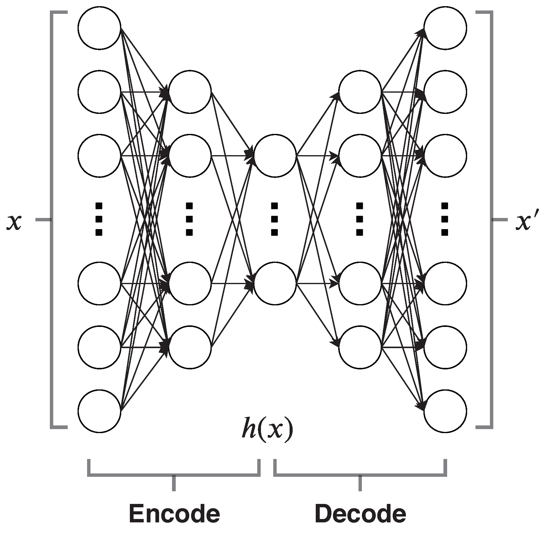
Rumelhart et al. [18] first introduced autoencoders in order to overcome the back propagation in unsupervised context using the input as the target. Autoencoders are categorised as self-supervised, since the input and the output are particularly the same [19]. As defined by Goodfellow et al. [20], an Autoencoder is “a neural network that is trained to attempt to copy its input to its output” [20]. Figure 1 illustrates the basic architecture of an autoencoder. The architecture of an autoencoder and the number of hidden layers differ based on the domain and the usage scenario.
Formally, given an input X , an autoencoder is trained in order to minimise the reconstruction error, as demonstrated in Equation (1) [19].
ϕ : X F ψ : F X ϕ , ψ = argmin ϕ , ψ | | X ( ϕ ψ ) X | | 2
such that ϕ and ψ represent the encoding and decoding functions, respectively.
Commonly, the reconstruction error of an input x is represented as the difference between x and x , such that:
x = g ( f ( x ) )
where f ( x ) is the encoding function, constructing the encoded vector of x; g ( x ) is the decoding function, restoring x to its initial value
The reconstruction error is defined by a function that represents the difference between the input x and the reconstructed input x . Mean square error and mean absolute error are common functions that are used in order to calculate the reconstruction error, as shown in Equations (2) and (3), respectively.
M S E = i = 1 N ( x x ) 2
M A E = i = 1 N | x x |
Supposing that the encoding function f ( x ) is single layer network with a linear function, the Autoencoder is viewed as equivalent to Principal Components Analysis (PCA) [21].
Autoencoders were originally used for dimensionality reduction and feature learning [22,23]. However, many other applications have been recently proposed. These applications include: word semantics [24], image compression [25], image anomaly detection [26], denoising [27], and others.

2.2. One-Class SVM

The SVM is one of the most well-established supervised ML techniques. Given the training samples, an SVM is trained to construct a hyperplane in a high-dimensional space that best separates the classes [28]. This hyperplane is a line in two dimensions case, a plane in the case of three dimensions (3D) or higher dimensions (n-dimensional). When data are not linearly separable, a kernel is used to map the input features/data to a non-linear higher dimensional space, in which a hyperplane would best separate the classes. The SVM kernels include; linear, polynomial, Gaussian, and Radial Basis Function (RBF).
Formally, given two classes, the minimisation problem of SVM is represented, as shown in Equation (4) [29].
min w R d | | w | | 2 + C i N max ( 0 , 1 y i f ( x i ) ) f ( x i ) = ( w T x i + b )
where C is a regularisation parameter to represent the trade-off between ensuring that x i is on the expected side of the plane and increasing the margin. Based on Equation (3), the data points fall in one of three places based on y i f ( x i ) . If  y i f ( x i ) is greater than 1, then the point is outside the margin and it does not contribute to the loss. If  y i f ( x i ) equals 1, then the point is on the margin. Finally, if  y i f ( x i ) is less than 1, then the point contributes to the loss, as it is on the wrong side [30].
In contrast to its supervised counterpart, the One-Class SVM is an unsupervised variant. It is defined as a model that is capable of detecting “Novelty” [31]. The goal of One-Class SVM is to fit a hyperplane that acts as a boundary which best includes all the training data and excludes any other data point. The result of training a One-Class SVM is seen as a spherically shaped boundary [32]. Because One-Class SVM is considered to be one of the most established outlier-based ML techniques, it provides an ideal comparison for assessing the performance of a deep neural network based autoencoder.
Formally, given a class with instances { x 1 , , x N } , and a mapping function φ ( ) that maps the features to a space H, the goal of One-Class SVM is to fit a hyperplane Π in H that has the largest distance to the origin, and all φ ( x i ) lie at the opposite side of hyper-plane to the origin [33].

3. Related Work

IDS is defined as “a system or software that monitors a network or systems for malicious activity”. Generally, IDSs can either be Network Intrusion Detection System (NIDS) or Host Intrusion Detection System (HIDS). NIDS monitors the network and communication while HIDS monitors the internal operation and log files [34]. Based on their detection techniques, IDSs are classified into Signature-based IDS, which relies on known signatures of prior and known attacks, and Anomaly-based IDS, which relies on patterns [35]. When compared to signature-based IDS, anomaly-based IDS perform better with complex attacks and unknown attacks.
In the past decade, researchers developed multiple techniques in order to enhance the robustness of anomaly-based IDS. Subsequent to a long period of using statistical methods to detect cyber anomalies and attacks, the need for ML emerged. Because of the sophistication of cyber-attacks, statistical methods were rendered inadequate to handle their complexity. Therefore, with the advancement of ML and DL in other domains (i.e., image and video processing, natural language processing, etc.), the researchers adopted these techniques for cyber use. Nguyen and Reddi [7] discuss the importance and benefit ML can provide to cybersecurity by granting a ‘robust resistance’ against attacks.
Based on the analysis of recent IDS research [36], ML has dominated the IDS research in the past decade. The analysis shows that Artificial Neural Networks (ANN), SVM, and k-means are the prevailing algorithms. Buczak and Guven [37] analyse the trends and complexity of different ML and DL techniques used for IDS. Moreover, recent research is directed towards the use of DL to analyse network traffic, due to the DL capabilities of handling complex patterns. Due to the complexity and challenges that are associated with encrypted traffic, building robust and reliable DL-based IDSs is crucial. Aceto et al. [38] describe this advancement in traffic encryption, as it ‘defeats traditional techniques’ that relies on packet-based and port-based data. At the beginning of 2019, 87% of traffic was encrypted [39], which emphasises on the growth and, thus the need for corresponding IDs. Research has utilised flow-based features as the building block for training and analysing IDSs in order to handle encrypted and non-encrypted traffic. The benefit of flow-based features, when compared to packet-based ones, relies on the fact that they can be used with both encrypted and unencrypted traffic and also they characterise high-level patterns of network communications. New DL approaches have recently been used to build robust and reliable IDS. One of these techniques is autoencoders.
In the cyber security domain, autoencoders are used for feature engineering and learning. Kunang et al. [40] used autoencoders for feature extraction, features are then passed into an SVM for classification. KDD Cup’99 and NSL-KDD datasets are both used for evaluation. The evaluation of the model, using autoencoder for feature extraction and SVM for multi-class classification, has an overall accuracy of 86.96% and precision of 88.65%. The different classes accuracies show a poor performance, as follows: 97.91%, 88.07%, 12.78%, 8.12%, and 97.47% for DoS, probe, R2L, U2R, and normal, respectively; a precision of 99.45%, 78.12%, 97.57%, 50%, and 81.59% for DoS, probe, R2L, U2R, and normal, respectively.
Kherlenchimeg and Nakaya [41] use a sparse autoencoder to extract features. The latent representation (the bottleneck layer of the autoencoder) is fed into a Recurrent Neural Network (RNN) for classification. The accuracy of the IDS model while using the NSL-KDD dataset is 80%. Similarity, Shaikh and Shashikala [42] focus on the detection of DoS attacks. They utilise a Stacked Autoencoder with an LSTM network for the classification. Using the NSL-KDD dataset, the overall detection accuracy is 94.3% and a false positive rate of 5.7%.
Abolhasanzadeh [43] used autoencoders for dimensionality reduction and the extraction of bottleneck feature. The experiments were evaluated while using the NSL-KDD dataset. In a similar fashion, Niyaz et al. [44] used autoencoders for unsupervised feature learning. They used the NSL-KDD dataset. Additionally, AL-Hawawreh et al. [45] used deep autoencoders and trained them on benign traffic in order to deduce the most important feature representation to be used in their deep feed-forward ANN.
Shone et al. [46] use a Stacked Non-Symmetric Deep Autoencoder to refine and learn the complex relationships between features that are then used in the classification using random forest technique. The authors used both the KDD Cup’99 and NSL-KDD datasets.
Farahnakian and Heikkonen [47] used a deep autoencoder to classify attacks. The deep autoencoder is fed into a single supervised layer for classification. Using the KDD Cup’99 dataset, the highest accuracies are 96.53% and 94.71% for binary and multi-class classification respectively.
In agreement with our manuscript, Meidan et al. [48] utilised the encoding-decoding capabilities of autoencoders to learn normal behaviour in IoT networks setup. Subsequently, IoT botnet and malicious behaviour are detected when the autoencoder reconstruction fails. Bovenzi et al. [49] emphasised the need for adaptive ML models to cope with the heterogeneity and unpredictability of IoT networks. The authors propose a two-stage IDS model, where they leverage the autoencoder capabilities in the first stage of their IDS.

4. Datasets

Two mainstream IDS datasets are chosen in order to evaluate the proposed models. The first is the CICIDS2017 dataset [50], which was developed by the Canadian Institute for Cybersecurity (CIC). The CICIDS2017 dataset covers a wide range of recent insider and outsider attacks. It comprises a diverse coverage of protocols and attacks variations and, finally, it is provided in a raw format which enables researchers the flexibility of processing the dataset. Therefore, the CICIDS2017 dataset is well-suited for evaluating the proposed models.
The CICIDS2017 dataset is a recording of a five-day benign, insider and outsider attacks traffic. The recorded PCAPs are made available. Table 1 summarises the traffic recorded per day. The raw files of the CICIDS2017 dataset are pre-processed, as described in Section 5.1. The full CICIDS2017 description and analysis is available in [51,52].
The second dataset is the NSL-KDD [53]. NSL-KDD was released by the CIC in order to overcome the problems of the KDD Cup’99 dataset [54]. The KDD Cup’99 dataset was the dataset of choice for evaluating more than 50% of the past decade IDS [36], followed by the NSL-KDD dataset, which was used for evaluating over 17% of IDS. However, the KDD Cup’99 has multiple drawbacks, as discussed thoroughly in [55]. These drawbacks include class imbalance and redundant records. Additionally, Siddique et al. [56] discussed the warnings provided to the UCI lab advising not to use KDD Cup’99 dataset in further IDS research. Consequently, NSL-KDD fits for the evaluation purpose of this manuscript, as well as the comparison with relevant research.
The NSL-KDD dataset covers normal/benign traffic and four cyber-attack classes, namely, Denial of Service (DoS), probing, Remote to Local (R2L), and User to Root (U2R). The NSL-KDD dataset is available in two files ‘KDDTrain+.csv’ and test file ‘KDDTest+.csv’. Similar to the KDD Cup’99, the NSL-KDD dataset is provided in comma separated value (csv) feature files. Each instance is represented with its feature values alongside the class label. The feature files undergo categorical features encoding to be appropriate for ML usage. The KDD Cup’99 and NSL-KDD datasets are analysed in [54]; furthermore, NSL-KDD is studied in [57].

5. Methodology, Approach and Proposed Models

In this section, the pre-processing of the datasets is discussed, followed by the explanation of the proposed, showing both the training and evaluation processes. Subsequently, Section 6 details the evaluation and results.

5.1. CICIDS2017 Pre-Processing

The process that is involved in preparing the CICIDS2017 dataset for use is described as follows. Firstly, ‘.pcap’ files of the CICIDS2017 dataset are split based on the attack type and the timestamps provided by the dataset. This process results in a separate ‘.pcap’ file for each attack class. Secondly, the ‘.pcap’ files are processed to generate bidirectional flows features. As highlighted by Rezaei and Liu [58], with the advancement and complexity of networks and relying on encrypted traffic, features need to be suitable for both encrypted and unencrypted traffic analysis. The authors also indicate that flow-based features are better-suited for modern IDS development. Based on the analysis of recent IDSs by Aceto et al. [38], flow and bidirectional flow features are the most commonly used. Thirdly, features with high correlation are dropped in order to minimise model instability. Algorithm 1 describes the process of dropping highly correlated features. A threshold of ‘0.9’ is used. Features with correlation less than the threshold are used for training. Finally, features are scaled using a Standard Scalar. It is important to mention that only benign instances are used in selecting the features and scaling in order to ensure zero influence of attack instances.
Algorithm 1 Drop correlated features
Input: Benign Data 2D Array, N, Correlation Threshold
Output: Benign Data 2D Array, Dropped Columns
1:
c o r r e l a t i o n _ m a t r i x d a t a . c o r r ( ) . a b s ( )
2:
u p p e r _ m a t r i x c o r r e l a t i o n _ m a t r i x [ i , j ]    { i , j N : i < = j }
3:
d r o p p e d i { i N : c o r r e l a t i o n _ m a t r i x [ i , * ] > t h r e s h o l d }
4:
d a t a d a t a . d r o p _ c o l u m n s ( d r o p p e d )
5:
return d a t a , d r o p p e d
As aforementioned, the goal is to train models using benign traffic and evaluate their performance to detect attacks. Therefore, normal/benign traffic solely is used for training. The normal instances are divided into 75% for training and 25% for testing/validation [59] by using sklearn train_test_split function with the shuffling option set to True (https://scikit-learn.org/stable/modules/generated/sklearn.model_selection.train_test_split.html). Furthermore, each of the attack classes then mimics a zero-day attack, thus assessing the ability of the model to detect its abnormality. Because the NSL-KDD dataset is split into training and testing, attacks in both files are used for evaluation.

5.2. Autoencoder-Based Model

The building block for the proposed Autoencoder is an Artificial Neural Network (ANN). For hyper-parameter optimisation, random search [60] is used in order to select the architecture of the network, number of epochs, and learning rate. Random search is known to converge faster than grid search to a semi-optimal set of parameters. It is also proved to be better than grid search when a small number of parameters are needed [61]. Finally, it limits the possibility of obtaining over-fitted parameters.
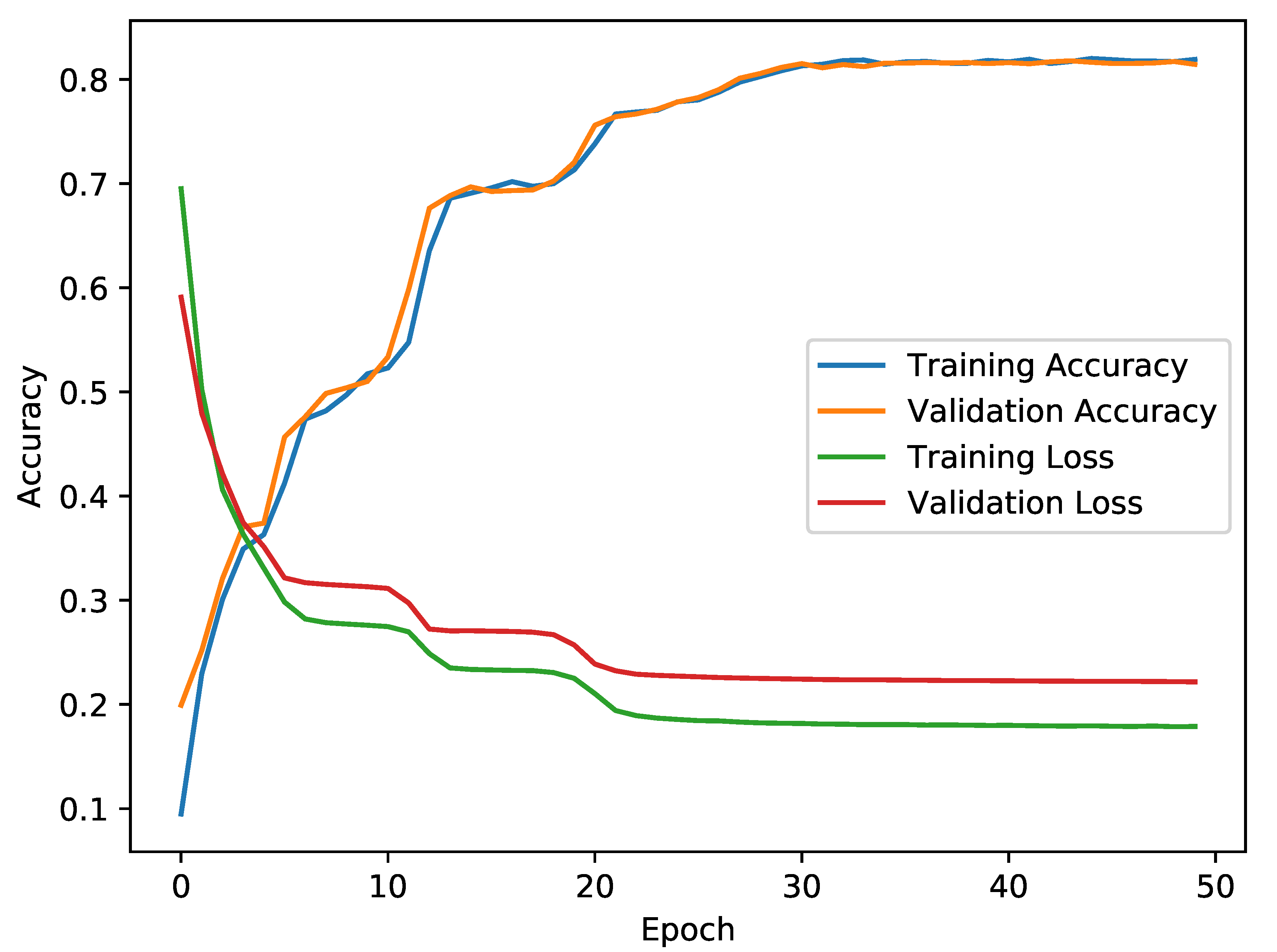
Once the hyper-parameters are investigated, the model is trained, as detailed in Algorithm 2. First, the benign instances are split into 75%:25% for training and validation, respectively. Subsequently, the model is initialised using the optimal ANN architecture (number of layers and number of hidden neurons per layer). Finally, the model is trained for n number of epochs. The loss and accuracy curves are observed in order to verify that the autoencoder convergence.
Once the model converges, as rendered in Figure 2, the model is evaluated using Algorithm 3. An attack instance is flagged as a zero-day attack if the Mean Squared Error (MSE) (reconstruction error) of the decoded ( x ) and the original instance (x) is larger than a given threshold. For the purpose of evaluation, multiple thresholds are assessed: 0.05, 0.1, 0.15. These thresholds are chosen based on the value that is chosen by the random search hyper-parameter optimisation. The threshold plays an important role in deciding the value at which an instance is considered a zero-day attack, i.e., what MSE between x and x is within the acceptable range.
Algorithm 2 Autoencoder Training
Input: benign_data, ANN_architecture, regularisation_value, num_epochs
Output: Trained Autoencoder
1:
t r a i n i n g = 75 % i b e n i g n _ d a t a
2:
t e s t i n g = b e n i g n _ d a t a t r a i n i n g ¯
3:
a u t o e n c o d e r b u i l d _ a u t o e n c o d e r ( A N N _ A r c h i t e c t u r e , r e g u l a r i s a t i o n _ v a l u e )
4:
b a t c h _ s i z e 1024
5:
a u t o e n c o d e r . t r a i n ( b a t c h _ s i z e , n u m _ e p o c h s , t r a i n i n g , t e s t i n g )
6:
return a u t o e n c o d e r
Algorithm 3 Evaluation
Input: Trained Autoencoder, attack, thresholds
Output: Detection accuracies
1:
d e t e c t i o n _ a c c u r a c i e s { }
2:
p r e d i c t i o n s m o d e l . p r e d i c t ( a t t a c k )
3:
for t h t h r e s h o l d s do
4:
   a c c u r a c y ( m s e ( p r e d i c t i o n s , a t t a c k ) > t h ) / l e n ( a t t a c k )
5:
   d e t e c t i o n _ a c c u r a c i e s . a d d ( t h r e s h o l d , a c c u r a c y )
6:
end for
7:
return d e t e c t i o n _ a c c u r a c i e s

5.3. One-Class SVM Based Model

One-Class SVM is trained using the benign instances. In order to train the One-Class SVM, a ‘ ν ’ value was specified. As defined by Chen et al., “ ν [0, 1], which is the lower and upper bound on the number of examples that are support vectors and that lie on the wrong side of the hyperplane, respectively”. [62]. The ν default value is 0.5, which includes 50% of the training sample in the hyperplane. However, for the purpose of this experiment, multiple ν values were chosen (0.2, 0.15, 0.1). These values were used in otder to evaluate and assess the autoencoder performance.
Algorithm 4 shows the process of training the One-Class SVM mode. Similar to the model that is discussed in Section 5.2, 75% of the benign samples are used to fit the One-Class SVM model. Unlike the Autoencoder model, where the evaluation relies on a threshold, a One-Class SVM trained model outputs a binary value {0,1}. The output represents whether an instance belongs to the class to which the SVM is fit. Hence, each attack is evaluated based on how many instances are predicted with a ‘0’ SVM output.
Algorithm 4 One-Class SVM Model
Input: benign_data, nu_value
Output: Trained SVM
1:
t r a i n i n g = 75 % i b e n i g n _ d a t a
2:
t e s t i n g = b e n i g n _ d a t a t r a i n i n g ¯
3:
o n e c l a s s s v m O n e C l a s s S V M ( n u _ v a l u e , r b f )
4:
o n e c l a s s s v m . f i t ( t r a i n i n g )
5:
return o n e c l a s s s v m

6. Experimental Results

6.1. CICIDS2017 Autoencoder Results

As mentioned, 75% of the benign instances is used to train the Autoencoder. The autoencoder optimised architecture for the CICIDS2017 dataset is comprised from an ANN network with 18 neurons in both the input and the output layers and 3 hidden layers with 15, 9, 15 neurons respectively. The optimal batch size is 1024. Other optimised parameters include mean square error loss, L2 regularisation of 0.0001 and for 50 epochs.
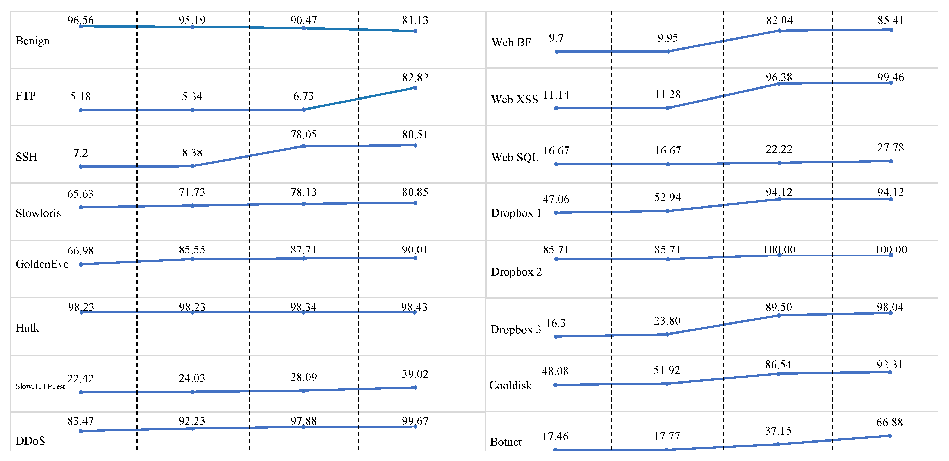
Figure 3 summarises the autoencoder accuracy of all CICIDS2017 classes. It is crucial to note that accuracy is defined differently for benign. Unlike attacks, for benign class, the accuracy represents the rate of instances not classified as zero-day (i.e., benign) which reflects the specificity and for the attack classes it represents the recall.
By observing Figure 3, benign accuracy is 95.19%, 90.47% and 81.13% for a threshold of 0.15, 0.1 and 0.05 respectively. Moreover, for the different attack detection accuracy, it is observed that there are three categories. Firstly, attacks that are very different from benign (for example, Hulk and DDoS), the detection accuracy is high regardless the threshold [92–99%]. Secondly, classes that are slightly different from benign (for example, SSH Brute-force and Port scanning), an accuracy rise is observed for lower thresholds. This emphasise the threshold’s role. Thirdly, classes that are not distinguishable from benign traffic, they are detected but with a lower accuracy (for example, Botnet, SQL Injection and DoS-SlowHTTPTest).
By observing Figure 3, different categories can be seen, (a) classes with a stable detection accuracy (i.e., line), and (b) classes with a prompt rise in detection accuracy in the right-most slice (0.05 threshold). Finally, the benign accuracy (top left) falls within an acceptable range with different thresholds.

6.2. CICIDS2017 One-Class SVM Results

Table 2 summarises the One-Class SVM results. By observing the One-Class SVM results, two assertions are identified, (a) the detection accuracy is not affected significantly by changing ν value, and (b) the classes with high detection accuracy in the Autoencoder results (Figure 3 are also detected by the One-Class SVM; however, the One-Class SVM fails to detect the two other categories (rise in detection accuracy with small thresholds and low detection accuracy). This is due to the limitations of the One-Class SVM algorithm which attempts to fit a spherical hyperplane to separate benign class from other classes, however, classes that fall into this hyperplane will always be classified as benign/normal.
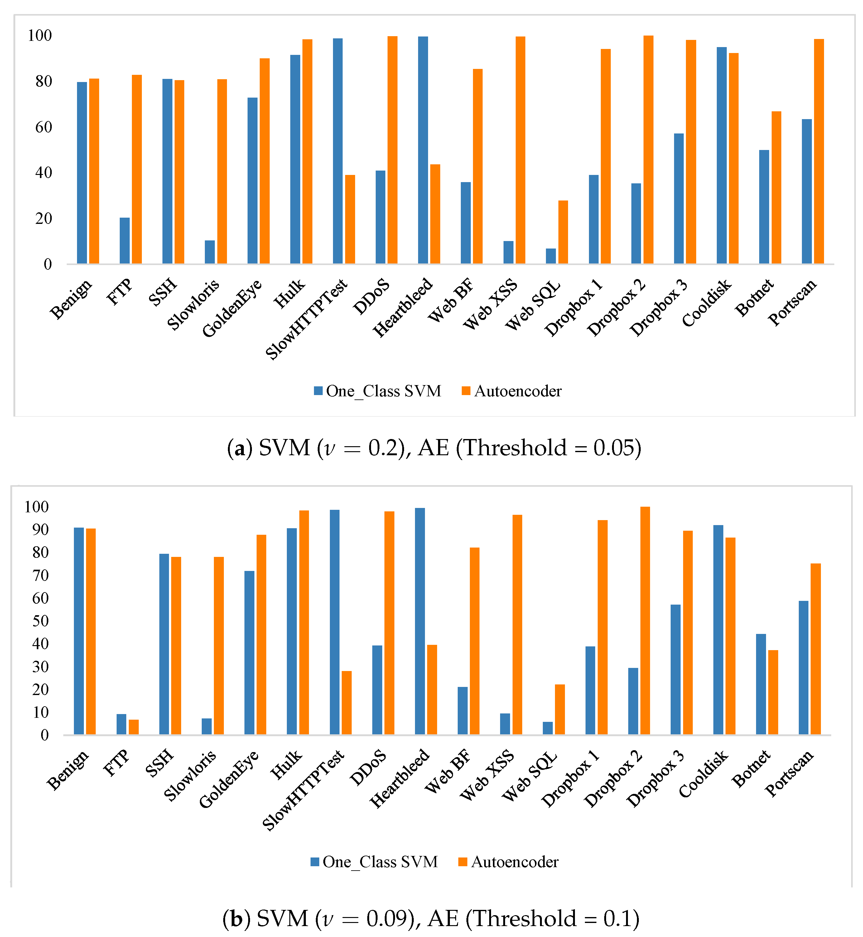
This can further be visualised in Figure 4. One-Class SVM is well suited for flagging recognisable zero-day attacks. However, autoencoders are better suited for complex zero-day attacks as the performance rank is significantly higher. Furthermore, Figure 4 shows a class by class comparison of the performance of autoencoder versus One-Class SVM. Figure 4a plots the results using One-Class SVM ν = 0.2 and autoencoder threshold of 0.05, while Figure 4b plots the results using One-Class SVM ν = 0.09 and autoencoder threshold of 0.1.

6.3. NSL-KDD Results

The autoencoder optimised architecture for the NSL-KDD dataset is comprised from an ANN network with 122 neurons in both the input and output layers and three hidden layers with 100, 60, 100 neurons, respectively. The optimal batch size is 1024. Other optimised parameters include mean absolute error loss, L2 regularisation of 0.001, and for 50 epochs.
Table 3 shows the autoencoder results for the NSL-KDD dataset. As aforementioned, attacks in both the KDDTrain+ and KDDTest+ files are used in order to evaluate the model. Similar to the results that are discussed in Section 6.1, the trade-off between the threshold choice and the true negative rate is observed.
Furthermore, when compared to the most recent available autoencoder implementation for detecting zero-day attacks in the literature [63], the autoencoder that is proposed in this manuscript largely outperforms the performances of [63]. The work proposed by Gharib et al. [63] used a hybrid two stage autoencoder to detect normal and abnormal traffic. Training on KDDTrain+ file and testing on KDDTest+, the overall accuracy of their proposed model is 90.17%, whereas the proposed autoencoder in this manuscript the overall accuracy is 91.84%, 92.96%, and 91.84% using a threshold of 0.3, 0.25, and 0.2, respectively. It is important to highlight that Gharib et al. [63] do not mention details regarding how they define anomalies or zero-day attacks or the classes they use in the testing process. Moreover, as summarised in Table 4, it is shown that the proposed approach in this manuscript outperforms the Denoising Autoencoder that is proposed in [64], specifically with the KDDTest+ instances with the authors accuracy is capped by 88%, while this manuscript reaches 93%.
Table 5 summarises the NSL-KDD One-Class SVM results. The results show a similar detection trend. This is due to the limited number and variance of attacks that are covered by the NSL-KDD dataset.

7. Conclusions and Future Work

The work that is presented in this manuscript proposes a new outlier-based zero-day cyber-attacks detection. The main goal was to develop an intelligent IDS model that is capable of detecting zero-day cyber-attacks with a high detection accuracy while overcoming the limitations of currently available IDS. This manuscript purposes and evaluates an autoencoder model to detect zero-day attacks. The idea is inspired by the encoding-decoding capability of autoencoders.
The results show high detection accuracy for the autoencoder model for both the CICIDS2017 and the NSL-KDD. The CICIDS2017 zero-day detection accuracy reaches 90.01%, 98.43%, 98.47%, and 99.67% for DoS (GoldenEye), DoS (Hulk), Port scanning, and DDoS attacks. Moreover, the NSL-KDD detection accuracy reached 92.96%, which outperforms the only available zero-day autoencoder-based detection manuscript [63].
Furthermore, the autoencoder model is compared to an unsupervised outlier-based ML technique; One-Class SVM. One-Class SVM is a prominent unsupervised ML technique that detects outliers. The one-class SVM mode presents its effectiveness in detecting zero-day attacks for NSL-KDD datasets and the distinctive ones from the CICIDS2017 dataset. When compared to One-Class SVM, autoencoder demonstrates its surpassing detection accuracy. Furthermore, both of the models demonstrate low miss rate (false-positives). Future work involves evaluating the proposed models with datasets that cover special purpose network IDS (e.g., IoT and Critical Infrastructure networks), which will comprise insights into adapting the proposed models, as well as proposing and adapting other ML techniques to use for zero-day attack detection. The source code for building and evaluating the proposed models will be made available through an open-source GitHub repository.

Author Contributions

Conceptualization, H.H., R.A. and X.B.; Formal analysis, H.H., R.A. and J.-N.C.; Investigation, H.H.; Methodology, H.H., R.A., C.T. and X.B.; Project administration, X.B.; Software, H.H.; Supervision, E.B. and X.B.; Validation, R.A., C.T., E.B. and X.B.; Writing—original draft, H.H.; Writing—review & editing, R.A., J.-N.C., E.B. and X.B. All authors have read and agreed to the published version of the manuscript.

Funding

This research received no external funding.

Conflicts of Interest

The authors declare no conflict of interest.

References

  1. Kaloudi, N.; Li, J. The AI-Based Cyber Threat Landscape: A Survey. ACM Comput. Surv. 2020, 53. [Google Scholar] [CrossRef] [Green Version]
  2. Hindy, H.; Hodo, E.; Bayne, E.; Seeam, A.; Atkinson, R.; Bellekens, X. A Taxonomy of Malicious Traffic for Intrusion Detection Systems. In Proceedings of the 2018 International Conference On Cyber Situational Awareness, Data Analytics and Assessment (Cyber SA), Glasgow, UK, 11–12 June 2018; pp. 1–4. [Google Scholar]
  3. Khraisat, A.; Gondal, I.; Vamplew, P.; Kamruzzaman, J. Survey of Intrusion Detection Systems: Techniques, Datasets and Challenges. Cybersecurity 2019, 2, 20. [Google Scholar] [CrossRef]
  4. Hindy, H.; Brosset, D.; Bayne, E.; Seeam, A.; Tachtatzis, C.; Atkinson, R.; Bellekens, X. A Taxonomy and Survey of Intrusion Detection System Design Techniques, Network Threats and Datasets. arXiv 2018, arXiv:1806.03517. [Google Scholar]
  5. Chapman, C. Chapter 1—Introduction to Practical Security and Performance Testing. In Network Performance and Security; Chapman, C., Ed.; Syngress: Boston, MA, USA, 2016; pp. 1–14. [Google Scholar] [CrossRef]
  6. Bilge, L.; Dumitraş, T. Before We Knew It: An Empirical Study of Zero-Day Attacks in the Real World. In Proceedings of the 2012 ACM Conference on Computer and Communications Security (CCS ’12), Raleigh, NC, USA, 16–18 October 2012; pp. 833–844. [Google Scholar] [CrossRef]
  7. Nguyen, T.T.; Reddi, V.J. Deep Reinforcement Learning for Cyber Security. arXiv 2019, arXiv:1906.05799. [Google Scholar]
  8. Metrick, K.; Najafi, P.; Semrau, J. Zero-Day Exploitation Increasingly Demonstrates Access to Money, Rather than Skill—Intelligence for Vulnerability Management; Part One; FireEye Inc.: Milpitas, CA, USA, 2020. [Google Scholar]
  9. Cisco. Cisco 2017 Annual Cyber Security Report. 2017. Available online: https://www.grouppbs.com/wp-content/uploads/2017/02/Cisco_2017_ACR_PDF.pdf (accessed on 20 July 2020).
  10. Ficke, E.; Schweitzer, K.M.; Bateman, R.M.; Xu, S. Analyzing Root Causes of Intrusion Detection False-Negatives: Methodology and Case Study. In Proceedings of the 2019 IEEE Military Communications Conference (MILCOM), Norfolk, VA, USA, 12–14 November 2019; pp. 1–6. [Google Scholar]
  11. Sharma, V.; Kim, J.; Kwon, S.; You, I.; Lee, K.; Yim, K. A Framework for Mitigating Zero-Day Attacks in IoT. arXiv 2018, arXiv:1804.05549. [Google Scholar]
  12. Sun, X.; Dai, J.; Liu, P.; Singhal, A.; Yen, J. Using Bayesian Networks for Probabilistic Identification of Zero-Day Attack Paths. IEEE Trans. Inf. Forensics Secur. 2018, 13, 2506–2521. [Google Scholar] [CrossRef]
  13. Zhou, Q.; Pezaros, D. Evaluation of Machine Learning Classifiers for Zero-Day Intrusion Detection–An Analysis on CIC-AWS-2018 dataset. arXiv 2019, arXiv:1905.03685. [Google Scholar]
  14. Zhao, J.; Shetty, S.; Pan, J.W.; Kamhoua, C.; Kwiat, K. Transfer Learning for Detecting Unknown Network Attacks. EURASIP J. Inf. Secur. 2019, 2019, 1. [Google Scholar] [CrossRef]
  15. Sameera, N.; Shashi, M. Deep Transductive Transfer Learning Framework for Zero-Day Attack Detection. ICT Express 2020. [Google Scholar] [CrossRef]
  16. Abri, F.; Siami-Namini, S.; Khanghah, M.A.; Soltani, F.M.; Namin, A.S. The Performance of Machine and Deep Learning Classifiers in Detecting Zero-Day Vulnerabilities. arXiv 2019, arXiv:1911.09586. [Google Scholar]
  17. Kim, J.Y.; Bu, S.J.; Cho, S.B. Zero-day Malware Detection using Transferred Generative Adversarial Networks based on Deep Autoencoders. Inf. Sci. 2018, 460–461, 83–102. [Google Scholar] [CrossRef]
  18. Rumelhart, D.E.; Hinton, G.E.; Williams, R.J. Learning Internal Representations by Error Propagation; Technical Report; California Univ San Diego La Jolla Inst for Cognitive Science: San Diego, CA, USA, 1985. [Google Scholar]
  19. Stewart, M. Comprehensive Introduction to Autoencoders. 2019. Available online: https://towardsdatascience.com/generating-images-with-autoencoders-77fd3a8dd368 (accessed on 21 July 2020).
  20. Goodfellow, I.; Bengio, Y.; Courville, A. Deep Learning; MIT Press: Cambridge, MA, USA, 2016. [Google Scholar]
  21. Barber, D. Implicit Representation Networks; Technical Report; Department of Computer Science, University College London: London, UK, 2014. [Google Scholar]
  22. Hinton, G.E.; Salakhutdinov, R.R. Reducing the Dimensionality of Data with Neural Networks. Science 2006, 313, 504–507. [Google Scholar] [CrossRef] [PubMed] [Green Version]
  23. Zabalza, J.; Ren, J.; Zheng, J.; Zhao, H.; Qing, C.; Yang, Z.; Du, P.; Marshall, S. Novel Segmented Stacked Autoencoder for Effective Dimensionality Reduction and Feature Extraction in Hyperspectral Imaging. Neurocomputing 2016, 185, 1–10. [Google Scholar] [CrossRef] [Green Version]
  24. Liou, C.Y.; Cheng, W.C.; Liou, J.W.; Liou, D.R. Autoencoder for Words. Neurocomputing 2014, 139, 84–96. [Google Scholar] [CrossRef]
  25. Theis, L.; Shi, W.; Cunningham, A.; Huszár, F. Lossy Image Compression with Compressive Autoencoders. arXiv 2017, arXiv:1703.00395. [Google Scholar]
  26. Zhou, C.; Paffenroth, R.C. Anomaly Detection with Robust Deep Autoencoders. In Proceedings of the 23rd ACM SIGKDD International Conference on Knowledge Discovery and Data Mining, Halifax, NS, Canada, 13–17 August 2017; pp. 665–674. [Google Scholar]
  27. Creswell, A.; Bharath, A.A. Denoising Adversarial Autoencoders. IEEE Trans. Neural Netw. Learn. Syst. 2018, 30, 968–984. [Google Scholar] [CrossRef] [PubMed] [Green Version]
  28. Cortes, C.; Vapnik, V. Support-Vector Networks. Mach. Learn. 1995, 20, 273–297. [Google Scholar] [CrossRef]
  29. Ng, A. Part V: Support Vector Machines|CS229 Lecture Notes. 2000. Available online: http://cs229.stanford.edu/notes/cs229-notes3.pdf (accessed on 21 July 2020).
  30. Zisserman, A. The SVM classifier|C19 Machine Learning. 2015. Available online: https://www.robots.ox.ac.uk/~az/lectures/ml/lect2.pdf (accessed on 21 July 2020).
  31. Schölkopf, B.; Williamson, R.C.; Smola, A.J.; Shawe-Taylor, J.; Platt, J.C. Support Vector Method for Novelty Detection. Adv. Neural Inf. Process. Syst. 2000, 12, 582–588. [Google Scholar]
  32. Tax, D.M.; Duin, R.P. Support Vector Data Description. Mach. Learn. 2004, 54, 45–66. [Google Scholar] [CrossRef] [Green Version]
  33. Wang, S.; Liu, Q.; Zhu, E.; Porikli, F.; Yin, J. Hyperparameter Selection of One-Class Support Vector Machine by Self-Adaptive Data Shifting. Pattern Recognit. 2018, 74, 198–211. [Google Scholar] [CrossRef] [Green Version]
  34. Hodo, E.; Bellekens, X.; Hamilton, A.; Tachtatzis, C.; Atkinson, R. Shallow and Deep Networks Intrusion Detection System: A Taxonomy and Survey. arXiv 2017, arXiv:1701.02145. [Google Scholar]
  35. Hamed, T.; Ernst, J.B.; Kremer, S.C. A Survey and Taxonomy of Classifiers of Intrusion Detection Systems. In Computer and Network Security Essentials; Daimi, K., Ed.; Springer International Publishing: Cham, Switzerland, 2018; pp. 21–39. [Google Scholar] [CrossRef]
  36. Hindy, H.; Brosset, D.; Bayne, E.; Seeam, A.K.; Tachtatzis, C.; Atkinson, R.; Bellekens, X. A Taxonomy of Network Threats and the Effect of Current Datasets on Intrusion Detection Systems. IEEE Access 2020, 8, 104650–104675. [Google Scholar] [CrossRef]
  37. Buczak, A.L.; Guven, E. A Survey of Data Mining and Machine Learning Methods for Cyber Security Intrusion Detection. IEEE Commun. Surv. Tutor. 2016, 18, 1153–1176. [Google Scholar] [CrossRef]
  38. Aceto, G.; Ciuonzo, D.; Montieri, A.; Pescapé, A. Toward effective mobile encrypted traffic classification through deep learning. Neurocomputing 2020, 409, 306–315. [Google Scholar] [CrossRef]
  39. Rashid, F.Y. Encryption, Privacy in the Internet Trends Report|Decipher. 2019. Available online: https://duo.com/decipher/encryption-privacy-in-the-internet-trends-report (accessed on 14 September 2020).
  40. Kunang, Y.N.; Nurmaini, S.; Stiawan, D.; Zarkasi, A.; Jasmir, F. Automatic Features Extraction Using Autoencoder in Intrusion Detection System. In Proceedings of the 2018 International Conference on Electrical Engineering and Computer Science (ICECOS), Pangkal Pinang, Indonesia, 2–4 October 2018; pp. 219–224. [Google Scholar]
  41. Kherlenchimeg, Z.; Nakaya, N. Network Intrusion Classifier Using Autoencoder with Recurrent Neural Network. In Proceedings of the Fourth International Conference on Electronics and Software Science (ICESS2018), Takamatsu, Japan, 5–7 November 2018; pp. 94–100. [Google Scholar]
  42. Shaikh, R.A.; Shashikala, S. An Autoencoder and LSTM based Intrusion Detection Approach Against Denial of Service Attacks. In Proceedings of the 2019 1st International Conference on Advances in Information Technology (ICAIT), Chickmagalur, India, 25–27 July 2019; pp. 406–410. [Google Scholar]
  43. Abolhasanzadeh, B. Nonlinear Dimensionality Reduction for Intrusion Detection using Auto-Encoder Bottleneck Features. In Proceedings of the 2015 7th Conference on Information and Knowledge Technology (IKT), Urmia, Iran, 26–28 May 2015; pp. 1–5. [Google Scholar]
  44. Javaid, A.; Niyaz, Q.; Sun, W.; Alam, M. A Deep Learning Approach for Network Intrusion Detection System. In Proceedings of the 9th EAI International Conference on Bio-Inspired Information and Communications Technologies (Formerly BIONETICS), New York, NY, USA, 3–5 December 2016; pp. 21–26. [Google Scholar]
  45. AL-Hawawreh, M.; Moustafa, N.; Sitnikova, E. Identification of Malicious Activities In Industrial Internet of Things Based On Deep Learning Models. J. Inf. Secur. Appl. 2018, 41, 1–11. [Google Scholar] [CrossRef]
  46. Shone, N.; Ngoc, T.N.; Phai, V.D.; Shi, Q. A Deep Learning Approach To Network Intrusion Detection. IEEE Trans. Emerg. Top. Comput. Intell. 2018, 2, 41–50. [Google Scholar] [CrossRef] [Green Version]
  47. Farahnakian, F.; Heikkonen, J. A Deep Auto-encoder Based Approach for Intrusion Detection System. In Proceedings of the 2018 20th International Conference on Advanced Communication Technology (ICACT), Chuncheon, Korea, 11–14 February 2018; p. 1. [Google Scholar]
  48. Meidan, Y.; Bohadana, M.; Mathov, Y.; Mirsky, Y.; Shabtai, A.; Breitenbacher, D.; Elovici, Y. N-BaIoT—Network-Based Detection of IoT Botnet Attacks Using Deep Autoencoders. IEEE Pervasive Comput. 2018, 17, 12–22. [Google Scholar] [CrossRef] [Green Version]
  49. Bovenzi, G.; Aceto, G.; Ciuonzo, D.; Persico, V.; Pescapé, A. A Hierarchical Hybrid Intrusion Detection Approach in IoT Scenarios. Available online: https://www.researchgate.net/profile/Domenico_Ciuonzo/publication/344076571_A_Hierarchical_Hybrid_Intrusion_Detection_Approach_in_IoT_Scenarios/links/5f512e5092851c250b8e934c/A-Hierarchical-Hybrid-Intrusion-Detection-Approach-in-IoT-Scenarios.pdf (accessed on 14 September 2020).
  50. Canadian Institute for Cybersecurity. Intrusion Detection Evaluation Dataset (CICIDS2017). 2017. Available online: http://www.unb.ca/cic/datasets/ids-2017.html (accessed on 15 June 2018).
  51. Panigrahi, R.; Borah, S. A Detailed Analysis of CICIDS2017 Dataset for Designing Intrusion Detection Systems. Int. J. Eng. Technol. 2018, 7, 479–482. [Google Scholar]
  52. Sharafaldin, I.; Habibi Lashkari, A.; Ghorbani, A.A. A Detailed Analysis of the CICIDS2017 Data Set. In Information Systems Security and Privacy; Mori, P., Furnell, S., Camp, O., Eds.; Springer International Publishing: Cham, Switzerland, 2019; pp. 172–188. [Google Scholar]
  53. Canadian Institute for Cybersecurity. NSL-KDD Dataset. Available online: http://www.unb.ca/cic/datasets/nsl.html (accessed on 15 June 2018).
  54. Tavallaee, M.; Bagheri, E.; Lu, W.; Ghorbani, A.A. A Detailed Analysis of the KDD CUP 99 Data Set. In Proceedings of the 2009 IEEE Symposium on Computational Intelligence for Security and Defense Applications, Ottawa, ON, Canada, 8–10 July 2009; pp. 1–6. [Google Scholar]
  55. Tobi, A.M.A.; Duncan, I. KDD 1999 Generation Faults: A Review And Analysis. J. Cyber Secur. Technol. 2018, 1–37. [Google Scholar] [CrossRef]
  56. Siddique, K.; Akhtar, Z.; Khan, F.A.; Kim, Y. Kdd Cup 99 Data Sets: A Perspective on the Role of Data Sets in Network Intrusion Detection Research. Computer 2019, 52, 41–51. [Google Scholar]
  57. Bala, R.; Nagpal, R. A Review on KDD CUP99 and NSL-KDD Dataset. Int. J. Adv. Res. Comput. Sci. 2019, 10, 64. [Google Scholar] [CrossRef] [Green Version]
  58. Rezaei, S.; Liu, X. Deep Learning for Encrypted Traffic Classification: An Overview. IEEE Commun. Mag. 2019, 57, 76–81. [Google Scholar] [CrossRef] [Green Version]
  59. Guggisberg, S. How to Split a Dataframe into Train and Test Set with Python. 2020. Available online: https://towardsdatascience.com/how-to-split-a-dataframe-into-train-and-test-set-with-python-eaa1630ca7b3 (accessed on 17 August 2020).
  60. Bergstra, J.; Bengio, Y. Random Search for Hyper-parameter Optimization. J. Mach. Learn. Res. 2012, 13, 281–305. [Google Scholar]
  61. Liashchynskyi, P.; Liashchynskyi, P. Grid Search, Random Search, Genetic Algorithm: A Big Comparison for NAS. arXiv 2019, arXiv:1912.06059. [Google Scholar]
  62. Chen, P.H.; Lin, C.J.; Schölkopf, B. A Tutorial on ν-Support Vector Machines. Appl. Stoch. Model. Bus. Ind. 2005, 21, 111–136. [Google Scholar] [CrossRef]
  63. Gharib, M.; Mohammadi, B.; Dastgerdi, S.H.; Sabokrou, M. AutoIDS: Auto-encoder Based Method for Intrusion Detection System. arXiv 2019, arXiv:1911.03306. [Google Scholar]
  64. Aygun, R.C.; Yavuz, A.G. Network Anomaly Detection with Stochastically Improved Autoencoder Based Models. In Proceedings of the 2017 IEEE 4th International Conference on Cyber Security and Cloud Computing (CSCloud), New York, NY, USA, 26–28 June 2017; pp. 193–198. [Google Scholar]
Publisher’s Note: MDPI stays neutral with regard to jurisdictional claims in published maps and institutional affiliations.
Figure 1. Autoencoder Architecture.
Electronics 09 01684 g001
Figure 2. Autoencoder Convergence Curves.
Electronics 09 01684 g002
Figure 3. CICIDS2017 Autoencoder Detection Results Summary Per Class.
Electronics 09 01684 g003
Figure 4. CICIDS2017 Autoencoder, One-Class SVM Comparison.
Electronics 09 01684 g004
Table 1. CICIDS2017 attacks.
DayTraffic
MondayBenign
TuesdaySSH & FTP Brute Force
WednesdayDoS/DDoS & Heartbleed
ThursdayWeb Attack (Brute Force, XSS, Sql Injection) & Infiltration
FridayBotnet, Portscan & DDoS
Table 2. CICIDS2017 One-Class Support Vector Machine (SVM) Results.
ClassAccuracy
ν 0.20.150.1
Benign (Validation)89.81%84.84%79.71%
FTP Bruteforce10.19%15.16%20.29%
SSH Bruteforce79.51%80.26%80.95%
DoS (Slowloris)7.66%8.38%10.37%
DoS (GoldenEye)71.87%72.39%72.85%
DoS (Hulk)90.69%91.35%91.55%
DoS (Slowhttps)98.59%98.66%98.71%
DDoS39.35%39.94%40.96%
Heartbleed99.49%99.54%99.58%
Web BF21.1%23.41%35.84%
Web XSS9.58%9.76%10.13%
Web SQL5.77%6.31%6.85%
Infiltration-Dropbox 138.89%38.89%38.89%
Infiltration-Dropbox 229.41%35.29%35.29%
Infiltration-Dropbox 357.14%57.14%57.14%
Infiltration-Cooldisk92.15%93.8%94.91%
Botnet44.23%46.15%50%
PortScan59.27%60.04%63.43%
Table 3. NSL-KDD Autoencoder Results.
ClassAccuracy
Threshold 0.30.250.2
KDDTrain+.csv
Normal (Validation)78.81%77.63%78.81%
DoS98.15%98.16%98.15%
Probe99.89%99.94%99.89%
R2L83.12%96.48%83.12%
U2R84.62%100%84.62%
KDDTest+.csv
Normal84.82%84.42%84.82%
DoS94.67%94.67%94.67%
Probe100%100%100%
R2L95.95%96.5%95.95%
U2R83.78%89.19%83.78%
Table 4. NSL-KDD Performance Comparison with Recent Literature. (Highest accuracy in Bold).
YearReferenceApproachTrain:Test % of KDDTrain+KDDTrain+ AccuracyKDDTest+ Accuracy
This paperAE th = 0.3
AE th = 0.25
AE th = 0.2
75 : 2588.92%
94.44%
88.92%
91.84%
92.96%
91.84%
2019[63]2 AEs--90.17%
2017[64]AE
Denoising AE
80 : 2093.62%
94.35%
88.28%
88.65%
Table 5. NSL-KDD One-Class SVM Results.
ClassAccuracy
ν 0.20.150.1
KDDTrain+.csv
Normal (Validation)89.9%85.14%80.54%
DoS98.13%98.14%98.14%
Probe97.74%98.77%99.52%
R2L49.35%52.26%81.71%
U2R78.85%80.77%82.69%
KDDTest+.csv
Normal88.12%86.02%84.72%
DoS94.67%94.67%94.69%
Probe99.55%99.91%100%
R2L80.17%82.22%90.31%
U2R78.38%78.38%83.78%