1. Introduction
A stereo correspondence algorithm uses a stereo image pair as an input and produces an estimated disparity map (a new image) as an output [
1,
2]. The estimation of a disparity map is a fundamental problem in computer vision. This problem has been addressed in multiple domains such as outdoor mapping and navigation [
3] and 3DTV [
4].
With additional information about the stereo vision system, a disparity map can be transformed into a map of distances. Therefore, in addition to the term disparity map, the terms range map and depth map also appear in the literature.
The accuracy of stereo correspondence algorithms can be assessed by the evaluation of disparity maps, either qualitatively or quantitatively. A quantitative (or objective) approach is robust against several human-related biasing factors, offering advantages over a qualitative (subjective) approach. This assessment has practical applications such as component and procedure comparison, parameter tuning, supports decision-making by researchers and practitioners, and in general, to measure the progress in the field. It is useful to be able to quantify the quality of these disparity maps in order to benchmark range-finding devices and stereo correspondence algorithms [
5].
Among the existing quantitative approaches used to estimate the accuracy/quality of disparity maps, Mean Squared Error (
MSE), Root Mean Squared Error (
RMSE) [
6], Mean Relative Error (
MRE) [
7], and the percentage of Bad Matched Pixels (
BMP) [
8] have been used extensively. A modification of the Multi-Scale Structural Similarity (
MS-SSIM) index for range image quality assessment was proposed in [
9], while the Sigma Z-Error (
SZE) objective measure was introduced in [
10]. The strengths of the
BMP and
MRE measures are combined in the Bad Matching Pixel Relative Error (
BMPRE) measure [
11].
The results of objective measures are used as inputs for quantitative evaluation methodologies, which aim to evaluate the performance of stereo algorithms. Among the existing quantitative evaluation methodologies, Middlebury’s methodology is commonly used [
12]. It uses the percentage of
BMP as the error measure. As an alternative to this evaluation methodology, the
groups methodology has been proposed [
13].
Among the current research in the field of stereo vision, disparity estimation based on deep learning methods [
14] and real-time disparity estimation for high-resolution images [
15] have been extensively studied, and significant progress has been made.
This paper proposes new disparity map evaluation measures, as modified versions of the original Image Quality Assessment (IQA) methods. The modification consists of the introduction of the capability to handle missing data in both the ground-truth disparity map (due to the lack of measures to determine ground-truth data) and in the estimated disparity map (due to the lack of an applied algorithm for image disparity estimation). The paper is focused also on consistency evaluation of the proposed measures using the two conceptually different state-of-the-art evaluation methodologies described in [
12,
13]. The obtained results show that the methodology extensions proposed in this research provide more accurate image disparity algorithm ranking.
The rest of this paper is organized as follows. The next section will describe the methodologies and dataset used for disparity maps’ evaluation. This is followed by the sections for experimental evaluation of known and the newly proposed objective error measures. The comparison of the results is shown in the next section. Finally, the conclusions are stated in the last section.
3. Disparity Evaluation Using Objective Measures
Although there are a number of techniques for assessing the similarity between two images [
18], simple pixel-based objective measures are generally used to assess the similarity between the ground-truth and the estimated disparity maps.
In most stereo applications, range images are obtained through range-finding devices or from structured light techniques. These methods often produce unknown regions (regions where the stereo algorithm fails to compute a depth estimate or regions where the range finder is shadowed by an obstacle). These unknown regions must be handled properly in order to obtain an accurate score from the quality metric. The local-based quality metric, termed
R-SSIM [
9], is capable of handling missing data in both the disparity map under evaluation and ground-truth data. Missing data in the disparity map may be associated with a fault of the stereo correspondence algorithm under evaluation.
In this section, pixel-based objective measures will be described first, and then, the local objective measures based on the Structural SIMilarity Index (
SSIM) [
19] will be introduced.
3.1. Disparity Evaluation Using Pixel-Based Objective Measures
The five commonly used pixel-based error measures are considered for the disparity map evaluation—
MSE,
MRE,
SZE,
BMP, and
BMPRE.
MSE is formulated as:
where
and
are the ground-truth and estimated disparity maps, respectively, and
N is the image size in pixels. However, the
MSE measure does not distinguish well between disparity estimates with a large number of small errors and disparity estimates with a small number of large errors.
The
MRE measure is formulated as:
while the
SZE measure is defined as [
10]:
where
f is the focal length,
B is the stereo system baseline (i.e., the distance between camera optical centers), and
is a constant added to avoid the instability due to missing estimations. In our research, it is assumed that
, while the value of the constant is
= 1. This measure is based on the inverse relation between disparity and depth using the magnitude of the disparity estimation error. It aims to measure the impact of a disparity estimation error on the 3D reconstruction. This impact depends on the true distance along the Z optical axis between the stereo camera system and the captured point and the point position according to the estimated disparity map.
The
BMP measure is formulated as [
12]:
where
is a binary function defined as:
and
is the error threshold, which was fixed to one pixel in our research (commonly used error threshold).
The
BMPRE measure is formulated as [
11]:
where
is a function defined in order to avoid divisions by zero:
is the disparity error magnitude, computed as the absolute difference between the estimated disparity and the true disparity value:
and
is the ratio between
and the true disparity value—the relative error:
The BMPRE measure considers, in a simple way, both the error magnitude and the inverse relation between depth and disparity. Moreover, the impacts of these considerations are not simple at all, since they allow a proper and deeper quantitative evaluation of disparity maps than the evaluation obtained using the BMP. In contrast to error measures that consider the inverse relation between depth and disparity (SZE), the BMPRE does not require additional information about the stereo camera system.
The pixel-based objective scores for the disparity maps of Tsukuba, Venus, Teddy, and Cones, estimated by the
PMF and the
ADCensus stereo correspondence algorithms [
12], are shown in
Table 1 (better objective scores of stereo algorithms for all stereo image pairs, criteria, and the complete dataset are highlighted in grey). The averaging of the 12 objective scores (4 stereo pairs × 3 criteria) points out the success of the algorithm on the global (dataset) level. These objective values can also be viewed as errors introduced by stereo algorithms (the lower, the better), i.e., the accuracy of the algorithms can be observed through them.
The obtained
PMF and
ADCensus scores using the
BMP measure are identical to the Middlebury stereo evaluation results [
12]. Furthermore, the
BMP and
BMPRE measures, for the Cones and the Teddy images, indicate a superior accuracy of the
PMF algorithm. On the contrary, they indicate a superior accuracy of the
ADCensus algorithm for the Tsukuba and the Venus images. On the other side, the
MRE scores indicate a superior accuracy of the
PMF algorithm. Although the
SZE and
MSE scores depend on the stereo image pair selection and criteria used, it can be concluded that the
PMF algorithm provides better disparity accuracy than the
ADCensus algorithm. If the accuracy of the disparity map is observed through the average value, based on the
BMP measure, the advantage is on the side of the
ADCensus algorithm, while for the remaining four objective measures, the
PMF algorithm provides a disparity map with better accuracy. Consequently, the selection of the error measure, in the evaluation process, has a great impact on the algorithm selection.
3.2. Disparity Evaluation Using SSIM-Based Objective Measures
The
SSIM index is a very popular algorithm for image quality evaluation. The basic idea behind the
SSIM technique is that the images of natural scenes are rich in structures and that the human eye is sensitive to structural distortions. The index describes the quality by comparing the local luminance (mean value), contrast (local variance), and structure (local correlation) between the reference and the test image using an 11 × 11 window [
19]. The dynamic range of this measure is [−1, 1]. The Universal Image Quality Index (
UIQI) [
20] is a special case of the
SSIM index. It is used to quantitatively assess a structural distortion between two images, and the dynamic range of this measure is also [−1, 1]. Both measures are calculated in the local regions of the image, using a moving window. The final quality indexes are obtained as the mean of all local quality values.
The Multi-Scale
SSIM or
MS-SSIM index [
21] is the most popular variation of the
SSIM index. It utilizes the
SSIM algorithm over several scales. The reference and distorted images are iteratively driven through a low-pass filter and down-sampled by a factor of two. The resulting image pairs are processed with the
SSIM algorithm. The
MS-SSIM algorithm compares details across resolutions in a multiplicative manner, providing the overall image quality score [
21].
The
R-SSIM algorithm is a variation of the
MS-SSIM algorithm with the ability to handle unknown regions or missing data in disparity maps’ evaluation [
9]. Treating unknown regions depends on their appearance—on the reference (ground-truth) image or on the distorted (estimated) image. Pixels in the unknown regions of the reference image should be ignored in objective measure calculations. Pixels in the unknown regions of the distorted image should be ignored when they fall inside the sliding window used to calculate the local objective value, but the objective value of the unknown pixels themselves should be set to zero.
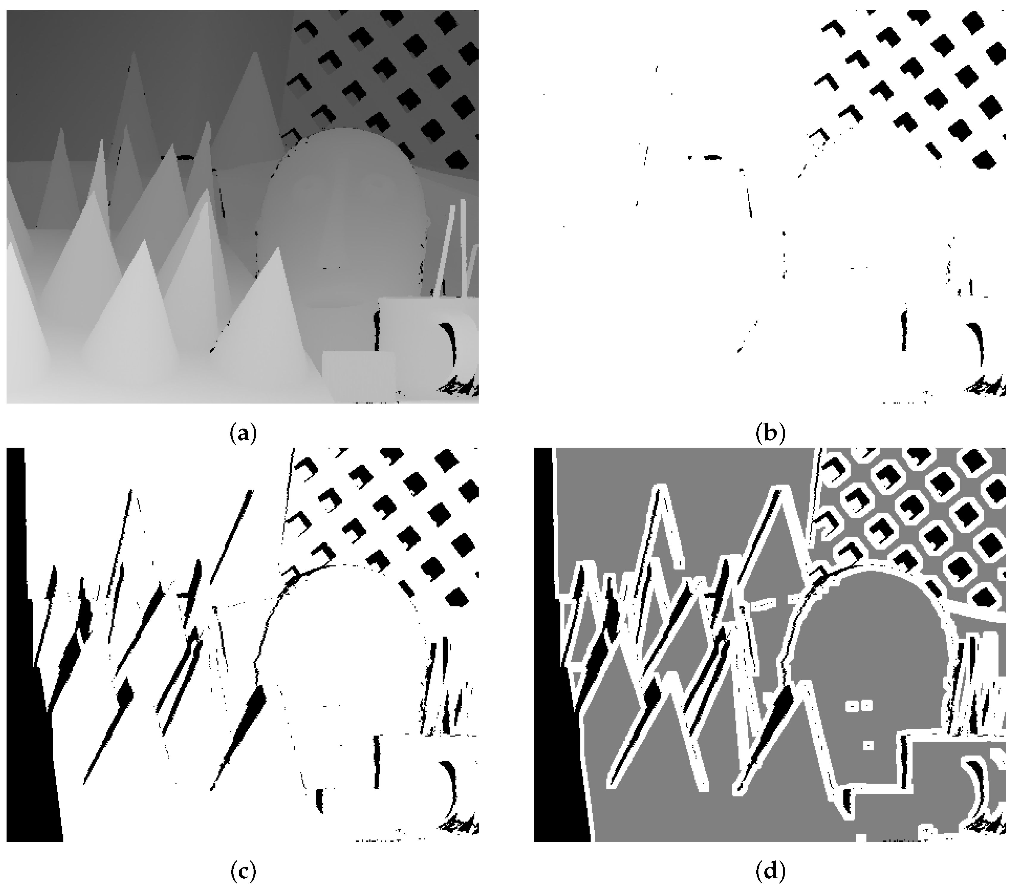
Figure 3 shows and explains how the
R-SSIM algorithm was implemented on one scale. The same idea in this research is applied for the
UIQI and
SSIM objective measures, and these modified measures we named as
and
.
Figure 3a depicts an 11 × 11 patch in the ground-truth (reference) disparity image where unknown pixels are shown in black.
Figure 3b shows the same patch in the estimated (test) disparity image, which also contains unknown (black) pixels.
Figure 3c shows the Gaussian weighting function, which is used in local
SSIM/
MS-SSIM calculations, and
Figure 3d shows it in the renormalized variant with ignored unknown (black) pixels. Finally,
Figure 3e shows a map of the
SSIM values of that patch, and
Figure 3f shows its modification, where the pixel in the middle was calculated from
Figure 3a,b,d. In
Figure 3f, the unknown region from
Figure 3b is indicated in black with a
SSIM score of zero, while the unknown region from
Figure 3a (shown in white) will be ignored in the final
R-SSIM score.
The
SSIM-based objective evaluations for the disparity maps of the Tsukuba, Venus, Teddy, and Cones images, estimated using the
AdaptWeight and the
TreeDP stereo correspondence algorithms [
12], are shown in
Table 2 (better objective scores of stereo algorithms for all stereo image pairs and complete dataset are highlighted in grey).
UIQI local scores are calculated using a sliding window of 8 × 8 pixels and a uniform weighting function [
20]. For these window-based measures, it is not reasonable to consider three criteria (
all,
nonocc, and
disc) used for pixel-based error measures [
9]. The averaging of the four stereo pairs’ obtained error scores points out the success of the algorithm on the global (dataset) level.
Generally, we can notice that the scores after the modification (, , and R-SSIM) are higher than the scores provided by the original objective measures (UIQI, SSIM, and MS-SSIM). Objective image quality measures without and with modification provide equal scores in situations where both disparity maps (ground-truth and algorithm computed) do not contain unknown regions (Venus image and AdaptWeight algorithm). Nevertheless, modified objective measures yield more real and precise results. Furthermore, it can be noticed that the objective measures give results that differ on the used algorithm and the selected image pair. Based on the objective measures, it can be concluded that the AdaptWeight algorithm provides disparity estimations that are closer to the ground-truth data than the TreeDP disparity map calculations.
Confirmation of the precedence of the
AdaptWeight stereo algorithm over the
TreeDP algorithm (measured by objective scores;
Table 2) can be seen in
Figure 4.
By visual inspection of the disparity maps from
Figure 4, it can be concluded that the disparity map obtained with the
AdaptWeight algorithm is closer to the ground-truth disparity map than the map obtained with the
TreeDP algorithm. Therefore, the objective similarity scores of the
AdaptWeight obtained map are higher than the
TreeDP generated one (
Table 2).
4. A New Local-Based Objective Measures for Disparity Evaluation
In this research, new objective measures are proposed for disparity image evaluation. Despite the SSIM-based objective measures, we used four state-of-the-art local-based objective image quality measures, which we adapted for range image quality assessment.
The gradient-based objective image quality assessment measure,
, is based on the preservation of gradient magnitudes and orientations [
22]. A comparison of gradient information is carried out at the local level in a 3 × 3 window, after which the local values of information preservation are used to determine the final quality score. As a result, a numerical
value is obtained that reflects the quality of the test image—the accuracy with which the original gradient information is presented in the test image. The
values are in the range [0, 1].
Gradient Magnitude Similarity Deviation (
GMSD) is also a gradient-based image quality assessment measure, which calculates a local similarity between the gradient magnitude maps of reference and test images in order to create a Local Quality Map (LQM) of the image degradation/similarity, in a 3 × 3 window. After this step, the standard deviation of the LQM is calculated in order to achieve a final image quality estimate:
GMSD [
23]. In this research, we used the mean value of the LQM (Gradient Magnitude Similarity Mean (
GMSM)) as a final quality score.
The Riesz transform and Visual contrast sensitivity-based feature SIMilarity index (
RVSIM) is a full reference IQA method, which combines Riesz transform and visual contrast sensitivity [
24].
RVSIM takes full advantage of the monogenic signal theory and log-Gabor filter by exploiting the contrast sensitivity function to allocate the weights of different frequency bands. At the same time, gradient magnitude similarity is introduced to obtain the gradient similarity matrix using a 3 × 3 window. Then, the monogenic phase congruency matrix is used to construct the pooling function and obtain the
RVSIM index.
Perceptual fidelity Aware
MSE (
PAMSE) is a variant of
MSE, produced by introducing an l2-norm structural error term to it, using a 7 × 7 Gaussian filter [
25]. Lower
PAMSE values indicate a higher similarity between the compared images, contrary to the other three local-based measures (
,
GMSM and
RVSIM) for which higher values indicate higher similarity.
For local-based objective measures , GMSM, RVSIM, and PAMSE, in this research, a new filtering method has been proposed to treat the unknown regions from disparity maps. Unlike the R-SSIM in which, for each pixel influenced by the unknown regions, a new computed value is calculated from the sliding window, in this approach, the new value for pixels affected by unknown regions is determined as the average value of valid (unaffected) local objective scores.
The range adapted objective measures, based on the four previously mentioned measures, are named in this research as
,
,
, and
.
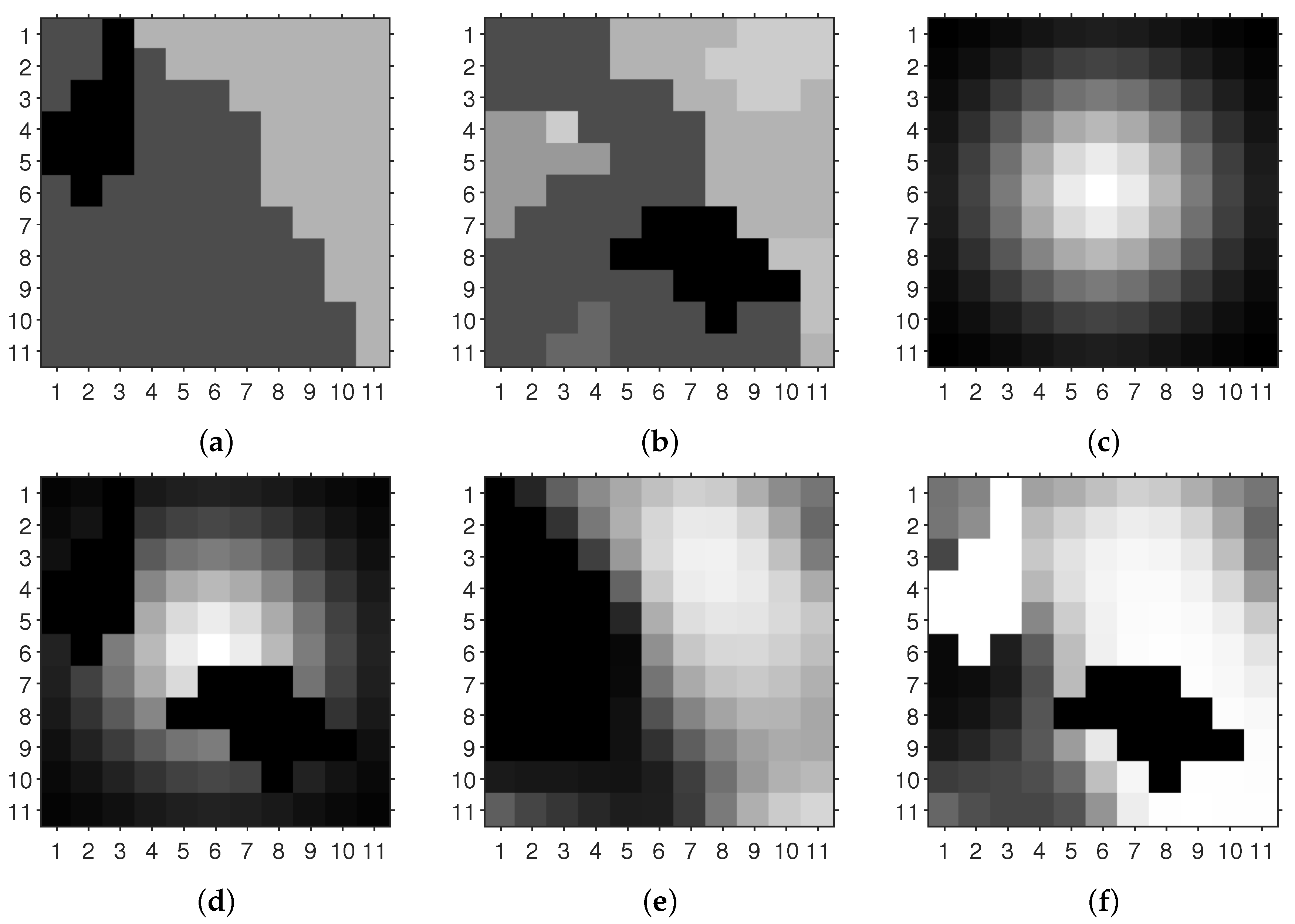
Figure 5 shows and explains how this adaptation was implemented for
GMSM, which is also valid for
and
RVSIM.
Figure 5a depicts a patch in the ground-truth (reference) image where there are some unknown pixels (shown in black), while
Figure 5b shows the same patch in the computed range image, which also contains unknown (black) pixels.
Figure 5c shows these unknown pixels and pixels affected by them (shown in white), in a 3 × 3 local-based objective calculations.
Figure 5d illustrates the proposed filtering method, where the objective score for the pixel numbered with one should be calculated from four local scores of unaffected pixels (shown as red squares), while the objective score for the pixel numbered with two should be the same as a local score of the only one unaffected pixel in a 3 × 3 neighborhood. Finally,
Figure 5e shows a map of the
GMSM values of that patch, and
Figure 5f shows its modification, where affected pixels were calculated using the proposed filtering method. In
Figure 5f, the same unknown region from
Figure 5b is indicated in black, with a
GMSM score of zero, while the unknown region in
Figure 5a (shown in white) will be ignored in the final
score. Since
PAMSE has an inverted scale (lower is better), the unknown pixels from the computed disparity image are penalized using the maximum disparity value, which is 255 for 8 bit/pixel grayscale images. Furthermore, for the PAMSE objective measure, it should be taken into account that the window size is 7 × 7 pixels, which will give a larger number of affected pixels.
The local-based objective evaluations for the disparity maps of the Tsukuba, Venus, Teddy, and Cones images, estimated using the
AdaptWeight and the
TreeDP stereo algorithms [
12], are shown in
Table 3 (better objective scores of stereo algorithms for all stereo image pairs and the complete dataset are highlighted in grey).
Image quality scores after the modification (
,
,
, and
) differ from image quality scores provided using original implementations that do not handle unknown regions (
,
GMSM,
RVSIM, and
PAMSE). Objective image quality measures without and with modification provide equal scores for the Venus image and the
AdaptWeight algorithm, for the same reason mentioned for the
SSIM-based measures—neither disparity map contains unknown regions. The results vary according to the choice of the objective algorithm, where the
AdaptWeight algorithm provides disparity estimations that are closer to the ground-truth data than the
TreeDP disparity map calculations (see
Figure 4), which is also valid for the previously described
SSIM-based objective measures (see
Table 2).
5. Results
In this research, fifty disparity stereo algorithms used in Middlebury’s dataset [
12] were analyzed, where 34 algorithms were used in [
9], and the 16 other algorithms were chosen among the state-of-the-art stereo algorithms. In order to perform image disparity algorithm evaluation, two methodologies were applied: Middlebury’s methodology and the
groups methodology.
The ranking of these algorithms using pixel-based objective measures was done by sorting the average ranks obtained for different stereo image pairs (Tsukuba, Venus, Teddy and Cones) and criteria (all, nonocc, and disc); this means that for the 12 rank values’ averaging while using SSIM-based and proposed local-based objective measures, the algorithms ranking was done by sorting the average ranks obtained for the four stereo image pairs (four ranking values averaging). The final algorithm rank was obtained by sorting the average ranks of all objective measures-based ranks.
A part of the ranked stereo correspondence algorithms according to Middlebury’s evaluation methodology (
BMP-based) and the rest of the considered objective measures are listed in
Table 4.
It can be observed that
Table 4 lists 20 different stereo algorithms, and the best one of them is
TSGO [
12], which is reported among the top-five by all objective measures’ rankings. Furthermore, it can be noticed that the algorithm rank in some cases differs significantly based on the objective measure used, i.e., the
IGSM algorithm is the best ranked according to the
BMP pixel-based measure, but it is ranked 25th using the
objective measure. This algorithm is positioned in 13th place on the global (final) level. For the bottom ranked algorithms (
DP,
SSD+MF,
PhaseDiff, and
SO [
12]), there is a high level of agreement between objective-based rankings.
The affiliation of the above 20 selected algorithms with
groups for the different objective error measures, according to the
groups methodology [
13], using 12 (pixel-based)/four (local-based) score errors, is shown in
Table 5. The lower label values identify the algorithms with better accuracy. The last row of the table shows the number of
subsets (labels) for each objective measure.
It can be seen that the first four average-based ranked stereo correspondence algorithms (
Table 4) are members of almost all the instances of the
sets. There are two exceptions: the
GC+LocalExp algorithm for the
measure and
PM-Forest for the
error measure. The worst average-based ranked algorithms belong to the
subsets with higher labels.
If we look at the individual ranks of the stereo correspondence algorithm
AdaptingBP (
Table 4), it can be concluded that this algorithm is positioned from first to 13th place. Based on all objective measures, it is in third place. The accuracy of this algorithm was better evaluated using the
groups methodology, where
Table 5 shows that it belongs to the
group by all objective measures.
The Linear Correlation (LC) between average error values of objective measures applied for all the 50 stereo correspondence algorithms is shown in
Table 6. From this table, it can be noticed that
SZE,
,
, and
have a weak mean correlation with the other objective measures (italicized scores in the last row). Moreover, we can see that proposed local-based measures
and
have a high correlation with the other measures (bolded scores in the last row). Knowing that
BMP and
BMPRE are the most frequently used measures in the literature (anchor points), we can see that the proposed
and
modifications can be good alternatives for them (bolded mutual scores), where
is computationally more efficient.
The correlation between objective measures can be illustrated through scatter plots.
Figure 6 shows the scatter plots of
and
, local-based objective error measures, versus
BMP and
BMPRE, pixel-based error measures, where each point (star) represents the average error of the utilized stereo algorithms (four values averaging for
/
and 12 values averaging for
BMP/
BMPRE). Scatter plots between these objective measures confirm the results given in
Table 6. It can be observed that
correlates better with
BMPRE (
Table 6, LC = 0.96) than
BMP (
Table 6, LC = 0.90). This can be explained by the fact that the
objective measure is also sensitive to disparity error magnitudes as the
BMPRE measure. For the disparity maps that are closer to the ground-truth (higher
and lower
BMP/
BMPRE values), the correlation between
and
BMP/
BMPRE objective measures is almost linear (in the upper left corner in the scatter plots). The degree of agreement between
and
BMP/
BMPRE is lower, which is visible through a big spreading of the objective scores on the scatter plots.
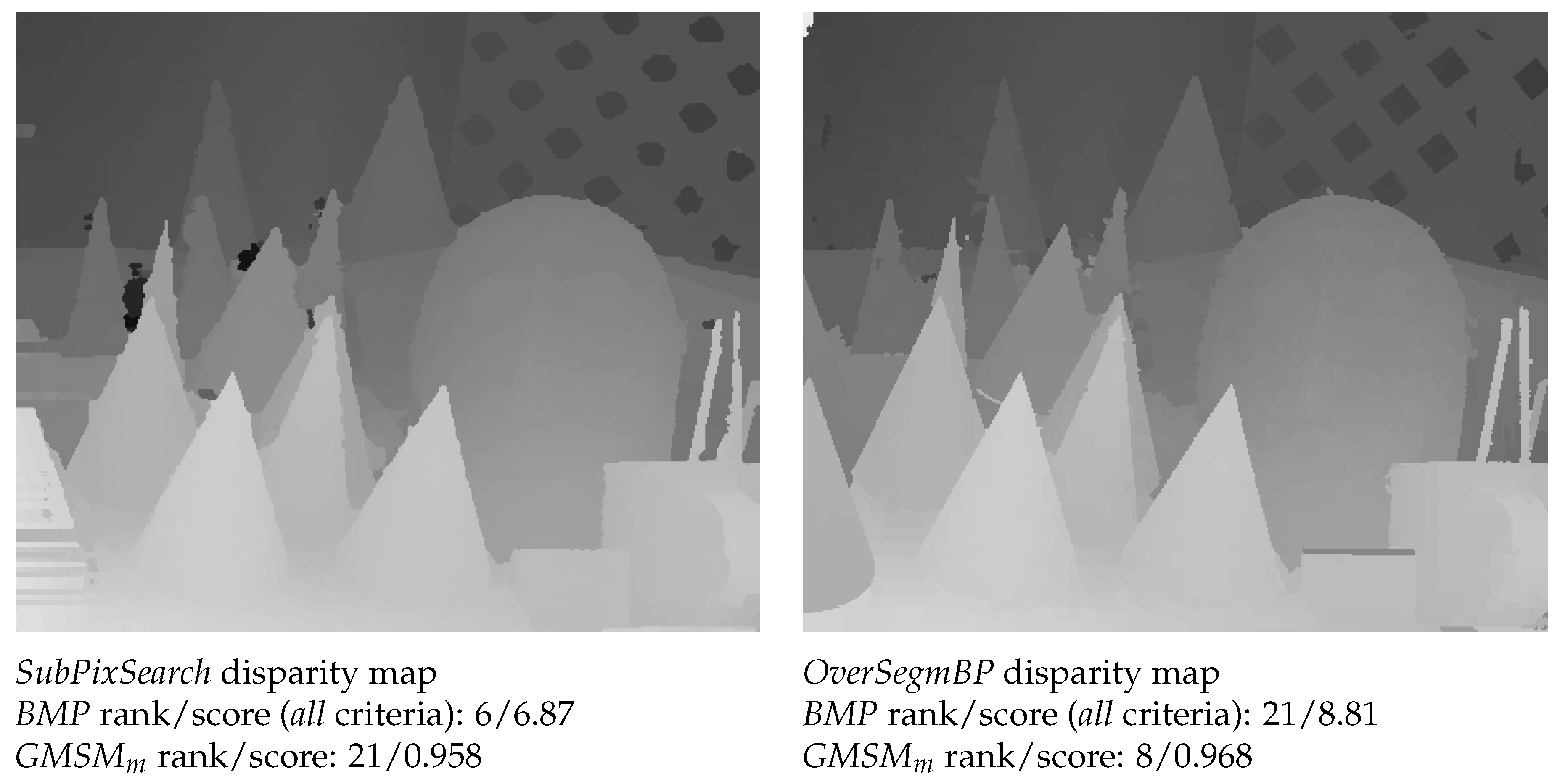
Figure 7 shows that the two objective methods can provide very different rankings to the same disparity maps. The two algorithms being assessed are graded in nearly reverse rank-order by the two assessment methods,
BMP and
. Therefore, in the performance analysis of stereo correspondence algorithms, it is desirable to use more objective quality measures. Visual inspection of the two disparity maps suggests that in this instance, the
algorithm delivers a more meaningful assessment of the quality of the estimated disparity map. Nevertheless, it can be noticed that the
objective values of quality are very close (0.958 vs. 0.968) and that the ranks are significantly different (21 vs. eight). Therefore, it is reasonable to use the
groups methodology in the performance analysis of stereo correspondence algorithms, because algorithms whose accuracy is close will be classified in the same group.
We make the results for all 50 stereo algorithms publicly available to the research community as three Excel files in
Supplementary Materials. These files contain extended results that are not presented in this paper: error scores for all analyzed stereo algorithms by all objective measures for each stereo pair and criteria, their rankings, and
groups subsets. Furthermore, in these files, researchers can find error scores before and after the proposed modifications for local-based objective measures.
6. Conclusions
In this paper, a characterization of error measures for evaluating disparity maps is presented. The impact on the results caused by the selection of the error measure was analyzed using Middlebury’s and the groups methodologies. This is the first attempt to analyze disparity maps using a plethora of pixel-based and local-based objective measures, using both methodologies.
We proposed modified objective measures as a new and needed quality metric for range images and demonstrated their utility by the evaluation of 50 stereo algorithms in the Middlebury Stereo Vision page, using four stereo image pairs with a rigid baseline. We confirmed that the new objective measures are effective for range image quality assessment; they complement the evaluation of stereo algorithms using conventional bad matched pixels approaches, but they can be stand-alone error measures. These modifications measure more than a loss of depth values; they are sensitive to errors in depth and surface structure, which cannot be measured using bad matched pixels approaches.
Experimental evaluations showed that the objective error measures may lead to different and contradictory ordinary rankings of stereo algorithms. These differences are less using the groups methodology, where this methodology makes a fair judgment about the algorithms’ accuracy. Consequently, the fair comparison of stereo correspondence algorithms may be a more difficult task than it has been considered so far.


