1. Introduction
Computer-aided diagnostic (CAD) systems refer to all the techniques that aim to consolidate the automation of the disease diagnostic process. These systems have gained tremendous interest since the unfolding of various machine learning methods in the past decades because of their ability to perform any automatic task in a very reliable way. One of the most challenging tasks regarding those CAD systems is the complete analysis and understanding of the images that represent biological organisms. In the case of autoimmune diseases, indirect immunofluorescence (IIF) on human epithelial type 2 (HEp-2) cell patterns is the most recommended diagnosis methodology [
1]. However, the manual analysis of the IIF images represents an arduous task that can take a substantial time. Moreover, the complexity of the images leaves an important part to the subjectivity of the pathologists, which can lead to some inconsistency in the diagnosis results [
2]. That is the reason why CAD systems have gained critical attention in the past years. These systems can assist pathologists during the diagnostic process, mainly for the automatic classification of the different types of HEp-2 cells.
Different methods have been discussed in the literature and especially the methods presented during the different editions of the HEp-2 cell classification contest held by the International Conference on Pattern Recognition (ICPR) [
3]. As a classical pattern recognition task, HEp-2 cell classification methods comprise a feature extraction or selection process that is followed by a classification one. Feature extraction remains the most important part of the procedure, because it consists of extracting the relevant information that can support an accurate discrimination of the different cell types. Commonly, we can distinguish two groups of methods in the literature: the conventional machine learning-based methods and the deep learning-based ones.
Conventional machine learning techniques entail hand-crafted features that are chosen for their capability of carrying relevant elements that are necessary for discrimination. Early efforts in that direction have been made by researchers such as Cataldo et al. [
4], who proposed the gray level co-occurrence matrix and the discrete cosine transform (DCT) features, and Wiliem et al. [
5], who adopted the codebooks generated from the DCT features and scale-invariant feature transform (SIFT) descriptors. Nosaka et al. [
6] used the local binary patterns (LBP) as the features and given them as inputs to a linear support vector machine (SVM) for the classification step. Huang et al. [
7] utilized the textural and statistical features in a hybrid fashion and fed them to a self-organizing map for the classification process.
Other statistical features, such as the gray-level size zone matrix, have been employed as the principal features in the work by Thibault et al. [
8] and the nearest-neighbor classifier was adopted for the discrimination part. The same statistical features have been fed to an SVM in the work of Wiliem et al. [
9], while a linear local distance coding method was used for extracting the features that were also utilized as the inputs of a linear SVM by Xu et al. [
10].
Hybrid feature learning methods have also been utilized by the researchers in this field. In fact, Cataldo et al. [
11] have proposed the use of a combination of different features such as morphological features, global texture descriptors like the rotation-invariant Gabor features [
12], and also different kinds of LBP descriptors like the rotation-invariant uniform LBPs [
13], the co-occurrence adjacent LBPs [
14], the completed LBP [
15], and also the rotation-invariant co-occurrence of adjacent LBPs, which are also adopted in [
6]. Another hybrid feature extraction method can be found in the work of Theodorakopoulos et al. [
16] where the authors proposed the combination of LBP and SIFT descriptors. Different other hand-crafted features can be seen in [
17,
18], and many others are listed in the quasi-exhaustive review made by Foggia et al. [
3]. We can note that the performance of these methods exclusively relies on the discrimination potentiality afforded by the extracted features, leaving, again, an important part to the subjectivity of the user.
Automatic feature learning methods have been widely adopted since the unfolding of deep learning [
19]. They have shown outstanding results in object recognition problems [
20,
21] and many researchers have adopted them as the principal tool for the HEp-2 cell classification. Unlike conventional methods, whose accuracy depends on the subjective choice of the features, deep learning methods, such as the now popular convolutional neural networks (CNNs), have the advantage of offering an automatic feature-learning process. In fact, many works have demonstrated the superiority of deep learning-based features over the hand-crafted ones for the HEp-2 cell classification task [
2,
22,
23,
24,
25,
26,
27,
28,
29,
30].
The first work to apply CNN to the HEp-2 cell classification problem was presented by Foggia et al. [
2] during the 2012 edition of the ICPR HEp-2 cell classification contest. Although the results were outstanding, the datasets available at that time were not heterogeneous enough and needed a lot of improvements. Since then, many available datasets have been significantly diversified and the different proposed CNN models continue to push the limits in terms of the classification accuracy. Gao et al. [
22] have presented a simple CNN architecture that was tested over different datasets. They were the first to test the data augmentation techniques, such as rotation in different angles, for the HEp-2 cell images. Li et al. [
23] have adopted the deep residual inception model, the DRI, which combines two of the most popular CNN models, the ResNet [
24] architecture and the “Inception” modules from the GoogleNet [
25]. Phan et al. [
26] have performed transfer learning, which consists of using an already trained network in a new dataset, by using a model that was trained on the ImageNet dataset.
A complex transfer learning method has been proposed by Lei et al. [
27] where they have used different proposed architectures of the pre-trained ResNet model and mixed it together in order to produce what they have named a cross-modal transfer learning approach. The results obtained via this method represent one of the state-of-the-art performances for the HEp-2 cell classification task. Another state-of-the-art performance was obtained in the work presented by Shen et al. [
28] where the authors used the ResNet approach again, but with a deeper residual module, called the deep-cross residual (DCR) module, with a huge data augmentation. Other CNN based methods can be seen in [
29,
30].
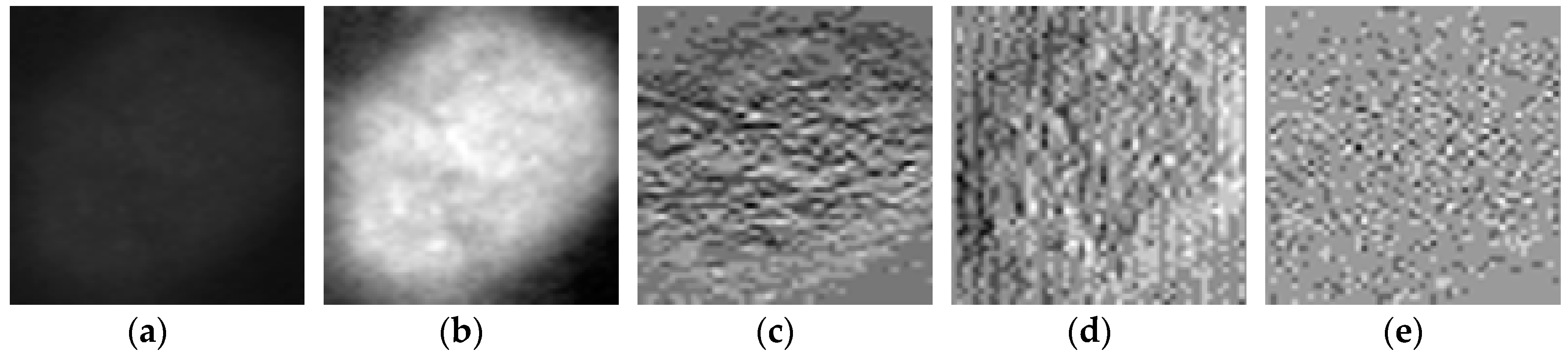
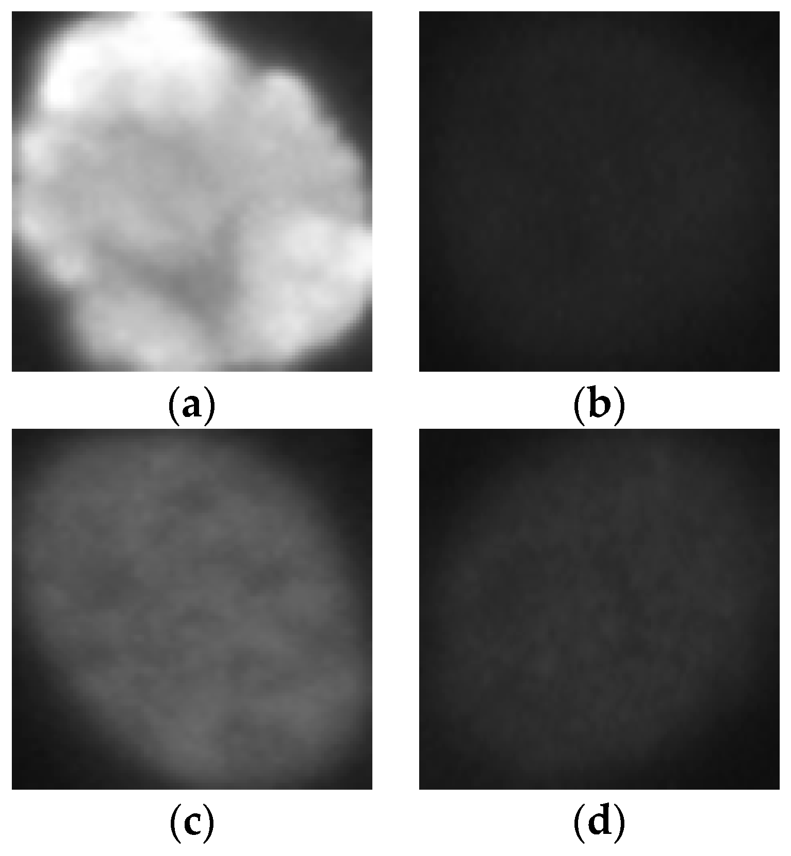
The HEp-2 cell images datasets generally denote a significant heterogeneity. This is explained by the intra-class variations caused by the existence of different intensity levels. In
Figure 1, we show some examples of the cellular images from one of the datasets used during the experiments. Both images in
Figure 1a,b represent the fine speckled cell type. The first image comes from the positive intensity level and the second one from the negative intensity level. The intra-class variations can be clearly seen from these two images that are supposed to belong to the same class. We can image the complexity faced by the classifiers that attempt to output these two images as from the same class. The heterogeneity discussed here becomes much clearer when we look at the images depicted in
Figure 1c,d. As for the previously mentioned type, both images belong to the same cellular type, the homogenous cells. Again, we can remark the intra-class variations. Moreover, the complexity becomes much noticeable when we compare the two negative intensity images shown in
Figure 1b,d. The two images are really similar in two main points: the lack of perceptibility of the cellular shape and the weakness of the illumination. Note that the two images, while being quite indistinguishable, are supposed to belong to two different classes.
This significant heterogeneity can cause certain problems in terms of the discrimination efficiency. Some of the actual state-of-the-art methods still encounter some trouble solving this problem, especially when the dataset exhibits a strong disparity. The method proposed in this work tries to specifically tackle this heterogeneity-related problem. We have chosen two datasets that show strong intra-class variations. Some methods, like the one proposed by Nigam et al. [
31], try to solve this problem by performing a preliminary intensity-based separation that precedes the cell type classification itself. Even though this way of proceeding can lead to reasonably good final results, the fact of using two steps in the classification part, after a burden future extraction process, clearly leads to elongating the global processing time. We propose a method that tries to minimize the heterogeneity in one step.
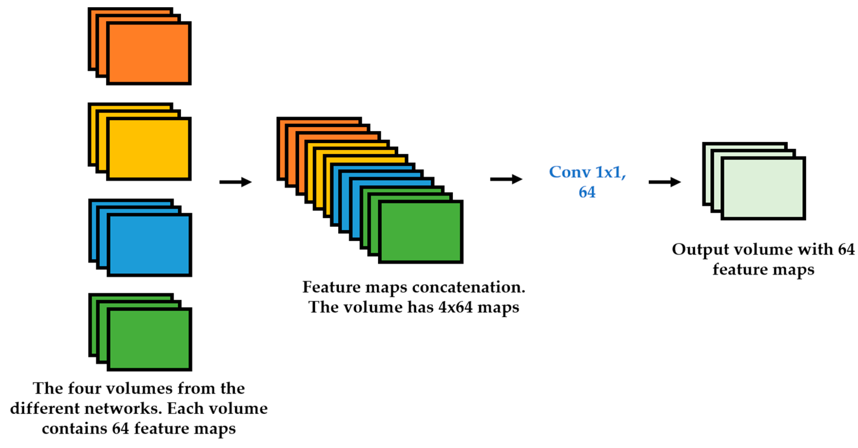
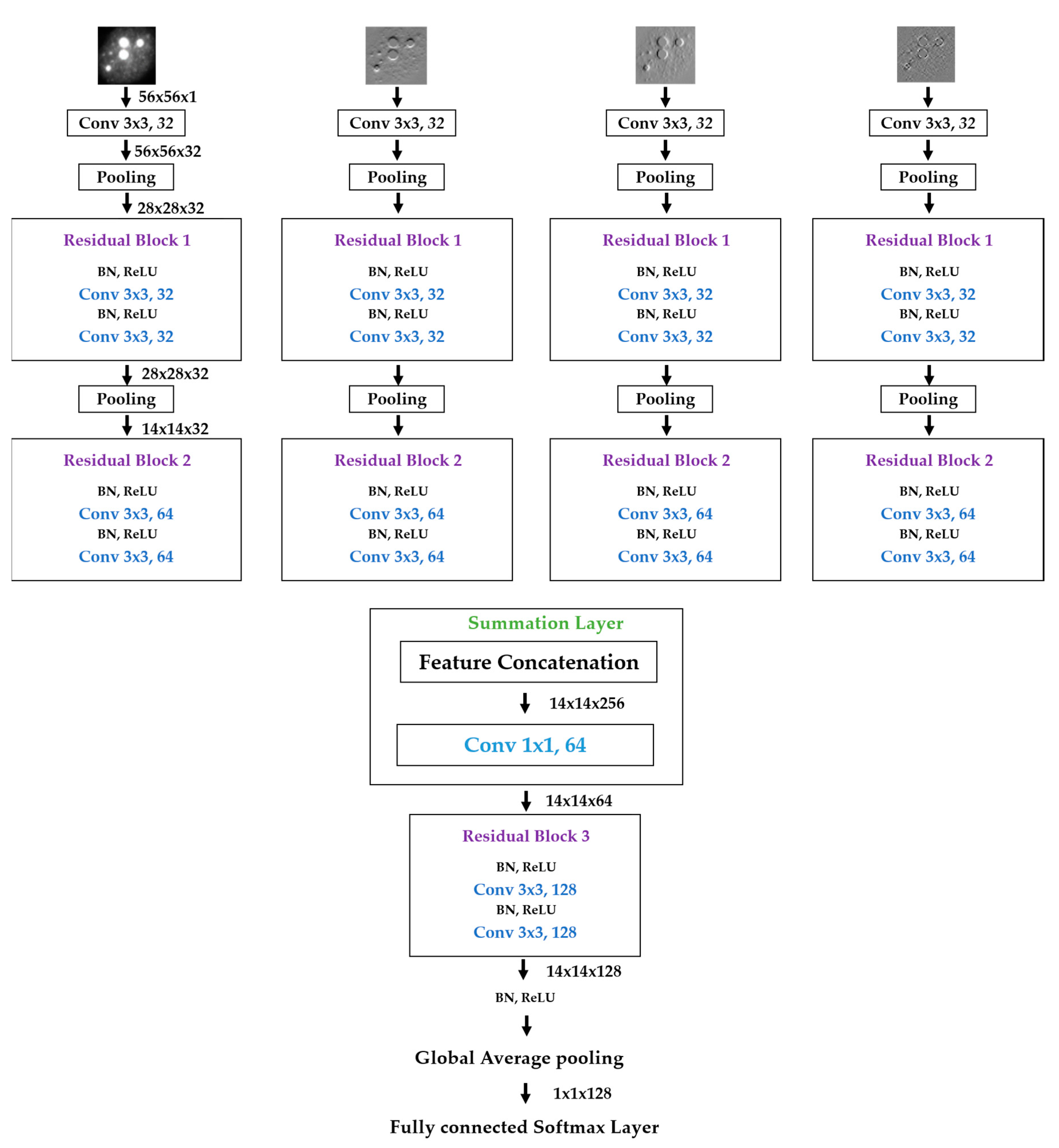
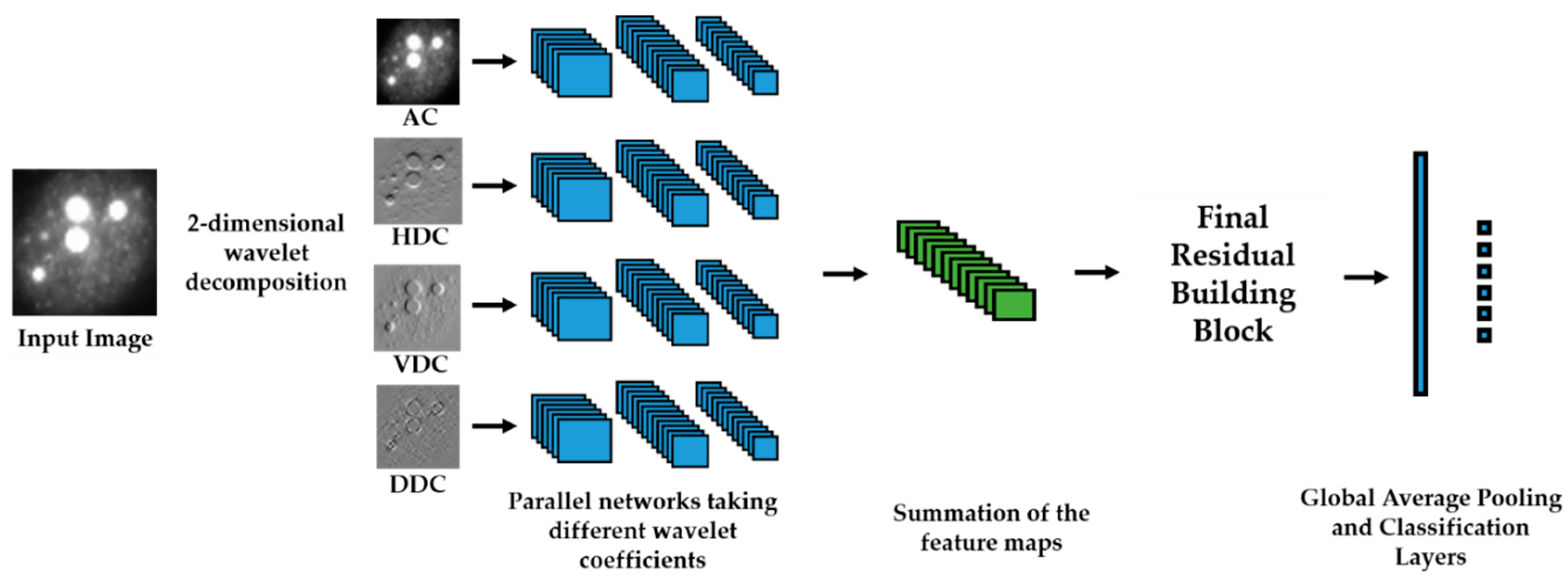
We propose a dynamic learning process with different networks taking different variations of the input image in parallel. The discrete wavelet transform (DWT) is used in order to produce the different variations. A two-dimensional DWT is performed over the images. The DWT coefficients are normalized and represented in an image form in order to feed the networks. Four different CNNs are used in parallel, each of them taking the different normalized wavelet coefficients as the inputs. The propagation of the error is done in parallel and, at a certain point of the networks, the high-level features from the feature maps of the four CNNs are concatenated and passed through a nonlinearity function in order mix up the different information learned by the four networks. Then, a final residual building block is formed using the output of the layer that performs the concatenation process. Finally, these nonlinearities are passed through a global average pooling layer and also a fully connected layer that will perform the final classification.
As explained in the next section, the different wavelet coefficients are expected to expose and significantly reinforce the localized changes in intensity, especially for the cellular types that exhibit strong differences in their levels of fluorescence illumination, thus, leading to a homogenization of not only the intensity, but also the shape, of the majority of the images of a given cell. The four different CNNs then learn dynamically these unveiled properties. The method was tested on the publicly available SNPHEp-2 [
5] and ICPR datasets and the results show that the strong disparity of the datasets is really minimized, thus, boosting the finally obtained discrimination results. The schematic representation of the proposed method is shown in
Figure 2.
The remaining content of the paper is organized as follows. The next section presents in detail each step of the proposed scheme.
Section 3 discusses about the obtained results and addresses a quasi-exhaustive comparative study using other methods.
3. Results
The proposed method was mainly tested on the SNPHEp-2 dataset. This dataset was obtained between January and February 2012 at the Sullivan Nicolaides Pathology laboratory at Australia. It contains five patterns: the centromere, the coarse speckled, the fine speckled, the homogeneous and the nucleolar types. The images depicted in
Figure 1, which represent the fine speckled and homogenous cells, were obtained from this dataset. It is composed of 40 different specimens and every single specimen image was captured using a monochrome camera, which was fitted on a microscope with a plan-Apochromat 20×/0.8 objective lenses and an LED illumination source. In order to automatically extract the image masks, which specifically delimit the cells’ body, the DAPI image channel was utilized.
There are 1884 cellular images in the dataset, all of them are extracted from the 40 different cells’ specimens. Different specimens were used for constructing the training and testing image sets, and both sets were created in such a way that they cannot contain images from the same specimen. From the 40 specimens, 20 were used for the training sets and the remaining 20 were used for the testing sets. In total, there are 905 and 979 cell images for the training and testing sets, respectively. Each set (training and testing) contains five-fold validation splits of randomly selected images. In each set, the different splits are used for cross-validating the different models and hyperparameters, each split containing 450 images approximatively. The SNPHEp-2 dataset was presented by Wiliem et al. [
5] and can be found at
http://staff.itee.uq.edu.au/lovell/snphep2/. Every cellular type from this dataset is represented by one example image in
Figure 9.
The ICPR 2016 [
36], on the other hand, dataset contains six different cellular types: the homogeneous (2494 images from 16 different specimens), the speckled (2831 images, 16 specimens), the nucleolar (2598 images, 16 specimens), the centromere (2741 images, 16 specimens), the nuclear membrane (2208 images, 15 specimens), and the Golgi (724 images, only 4 specimens). The dataset contains in total 13,596 images and can be downloaded at
http://mivia.unisa.it/datasets/biomedical-image-datasets/hep2-image-dataset/.
The choice of mainly using the SNPHEp-2 dataset for the results shown in this work was justified by the fact that it exhibits a significant heterogeneity compared to the ICPR one, which makes it pose serious problems for the discrimination. The dataset contains only around 2000 images, but 40 different cells’ specimens were used in order to produce these images. Besides the fact that the different sets (training and testing) comprise images from totally different specimens, the probability of finding many images that derive from the same specimen is significantly low. By comparison, the ICPR dataset, on which we have also tested the method and shown the results (only for the comparative study with the state-of-the-art methods), contains more than 10,000 images, but all of them were produced using only 83 specimens. There is a high probability to find in this dataset several images that derive from the same specimen. This fact reduces the heterogeneity of the dataset, making it susceptible to pose less complexity in terms of the discrimination compared to the SNPHEp-2. Note that, besides the fact that it contains more than 10,000 images, the ICPR dataset also exhibits strong complexity. We have just found that the complexity related to the variation of the fluorescence illumination, which is precisely the main problem that the proposed method aims to tackle, is more noticeable in the SNPHEp-2 dataset.
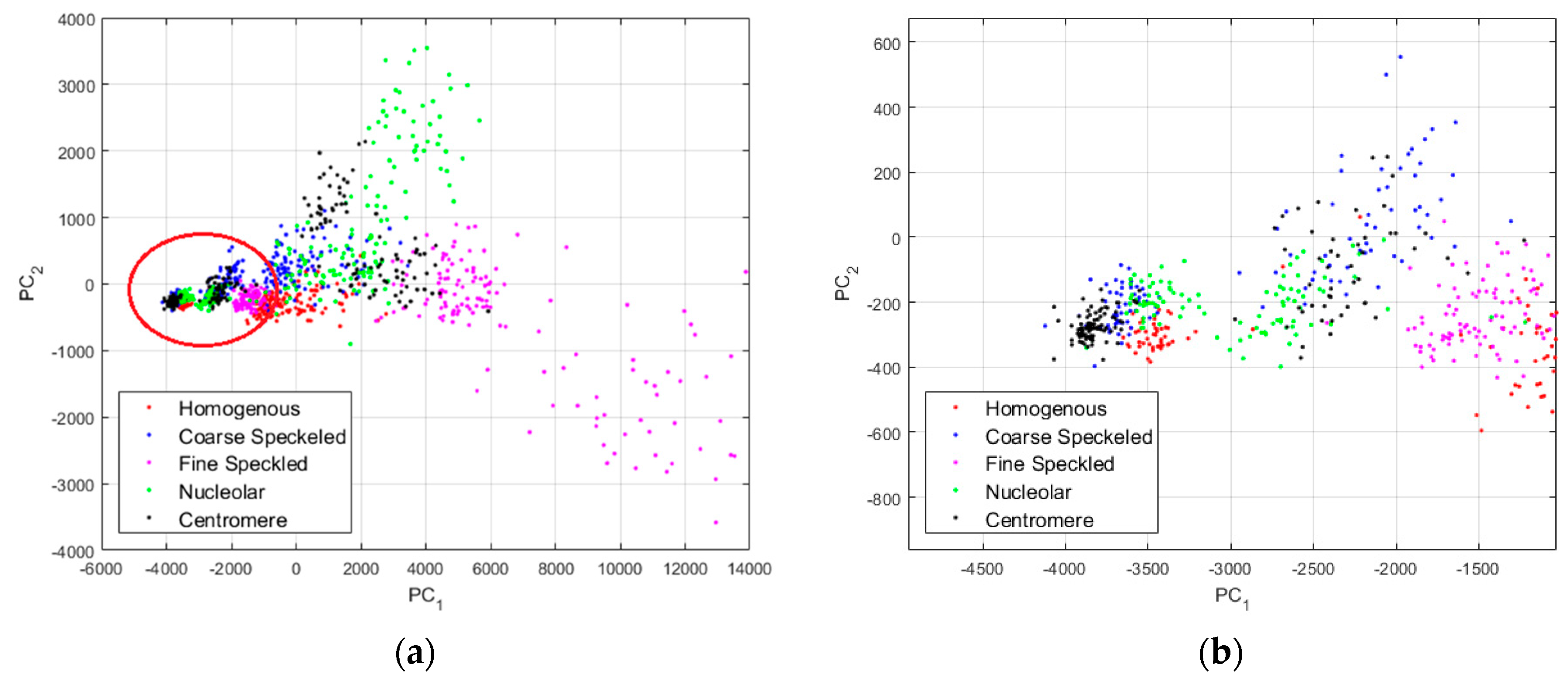
In
Figure 10, we show the projections of the data from this dataset using the principal component analysis (PCA) [
37]. PC
1 and PC
2 denote the first and second principal component axis, respectively. All the projections are shown in
Figure 10a, where we can clearly distinguish two main projection’s sub-spaces. Many data points, the positive intensity ones, are spread all around the PCA space, denoting their high heterogeneity. Specifically, the fine speckled cells, represented by the magenta dots, are scattered all over the PCA space. The projection sub-space that is surrounded by the red circle in
Figure 10a represents the negative intensity data. We have zoomed this part and shown the result in
Figure 10b. All the cellular types are present in that part of the PCA-space (see
Figure 10b), and they represent the negative intensity subset. At the same time, all the cellular types are also present in the other part (outside of the red circle), and they represent the positive intensity subset. The purpose of the proposed method is to try to minimize this heterogeneity by homogenizing the images from the same class but belonging to the different fluorescence illumination’s subsets.
Concerning the hyperparameters used during the training, different scenarios were used in order to optimize the discrimination results. These hyperparameters were selected via cross-validation using different splits, as clearly explained previously. All the following values concerning the hyperparameters are the ones that have provided the best results during the experiments. The initial learning rate was set to be 0.1 at the beginning of the training process. This value was then divided by a factor of 10 every 50 epochs. This schedule, as usually done in the literature with deep learning structures, aims to update the weights quickly at the beginning of the training process while the loss (error) is quite big, and then slowing down the update process, by decreasing the learning rate, when the loss decreases. The learning is terminated when the loss plateaus and does not change after decreasing the learning rate. The size of the mini-batch was set to be 128. The momentum was set to 0.9 and we have initialized the weights by following the process presented by He et al. [
33]. All the experiments were conducted with MATLAB R2018b and performed on a computer with a Core i7 3.40 GHz processor and 8 GB of RAM. A GPU implementation was used with a NVIDIA GeForce GTX 1080 Ti with 11,264 MB of memory, which accelerates the training time.
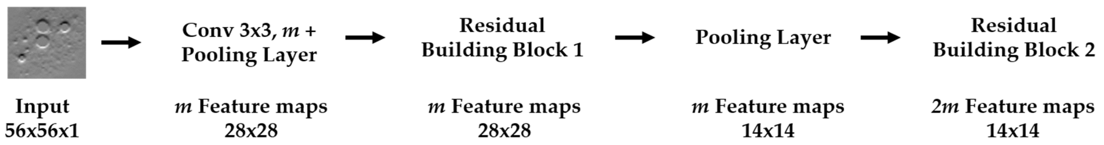
We start by the results obtained using one single network that takes the original images as the input. The structure of this network follows the same structure of the proposed method, except the fact that there is no summation layer because there is only a single network. The network structure is depicted in
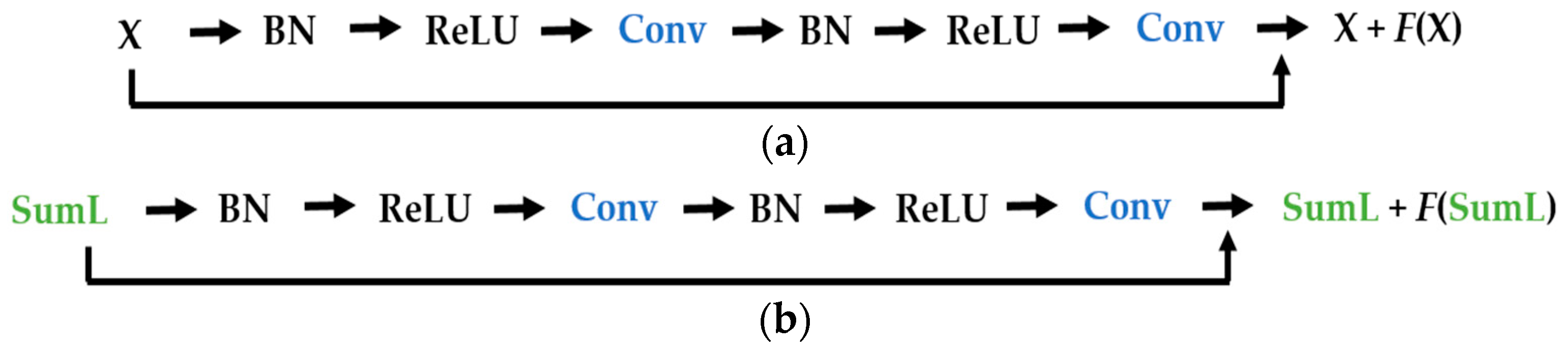
Figure 11. The original images are given to a convolution layer that is followed by three residual building blocks. The residual blocks have the same structure as the ones described in
Figure 6a. As previously mentioned, the original images have a size of 112 × 112, which is why the input, in this case, has that same size. Note that the input images of our parallel networks have a size of 56 × 56 because of the down-sampling process performed by the DWT decomposition at the first level.
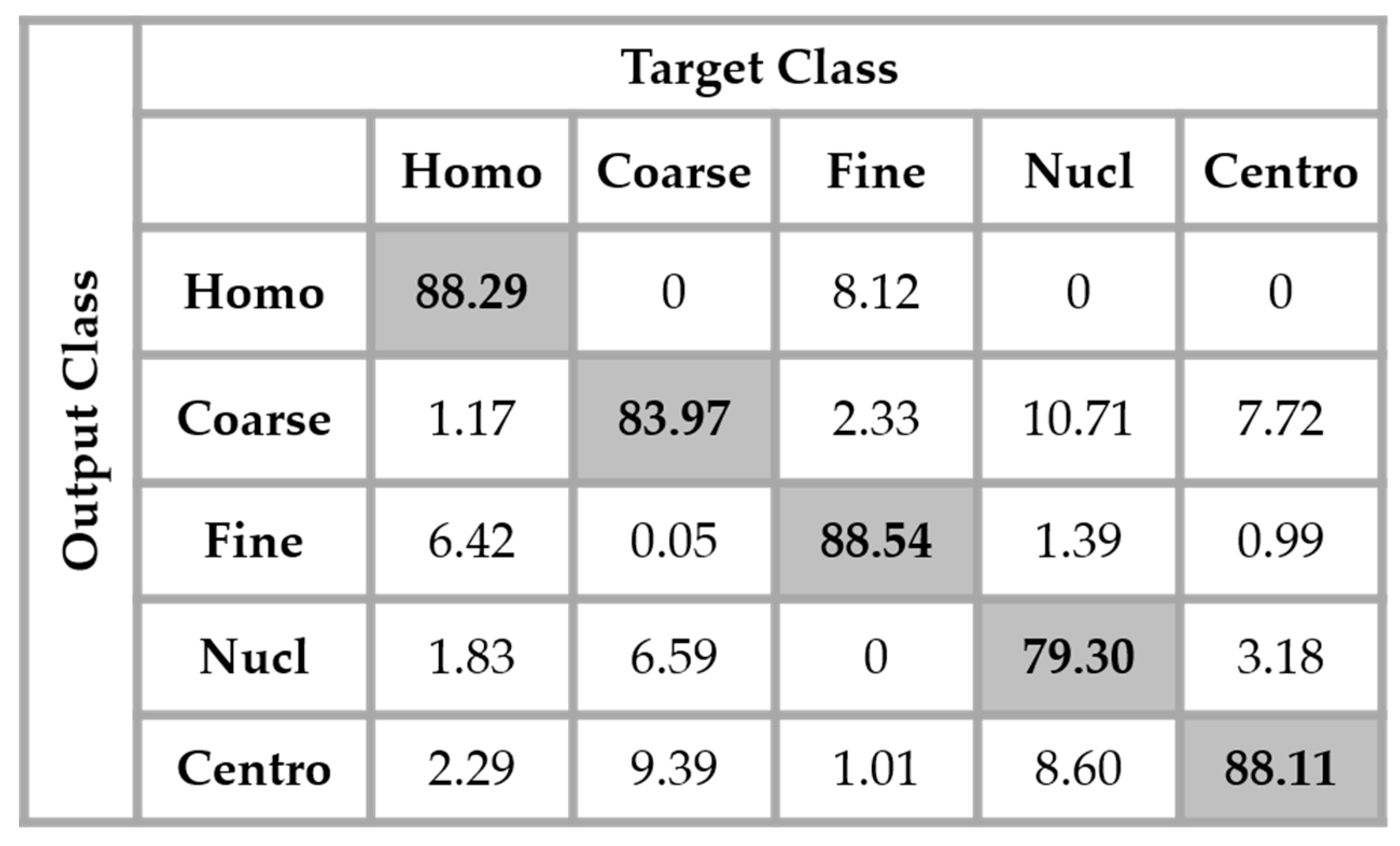
The results are shown in the confusion matrix denoted in
Figure 12. The same hyperparameters previously presented were used for training the single network. In all the confusion matrices shown in this work, “Homo”, “Coarse”, “Fine”, “Nucl”, and “Centro” denote, respectively, the homogeneous, coarse speckled, fine speckled, nucleolar and centromere cells.
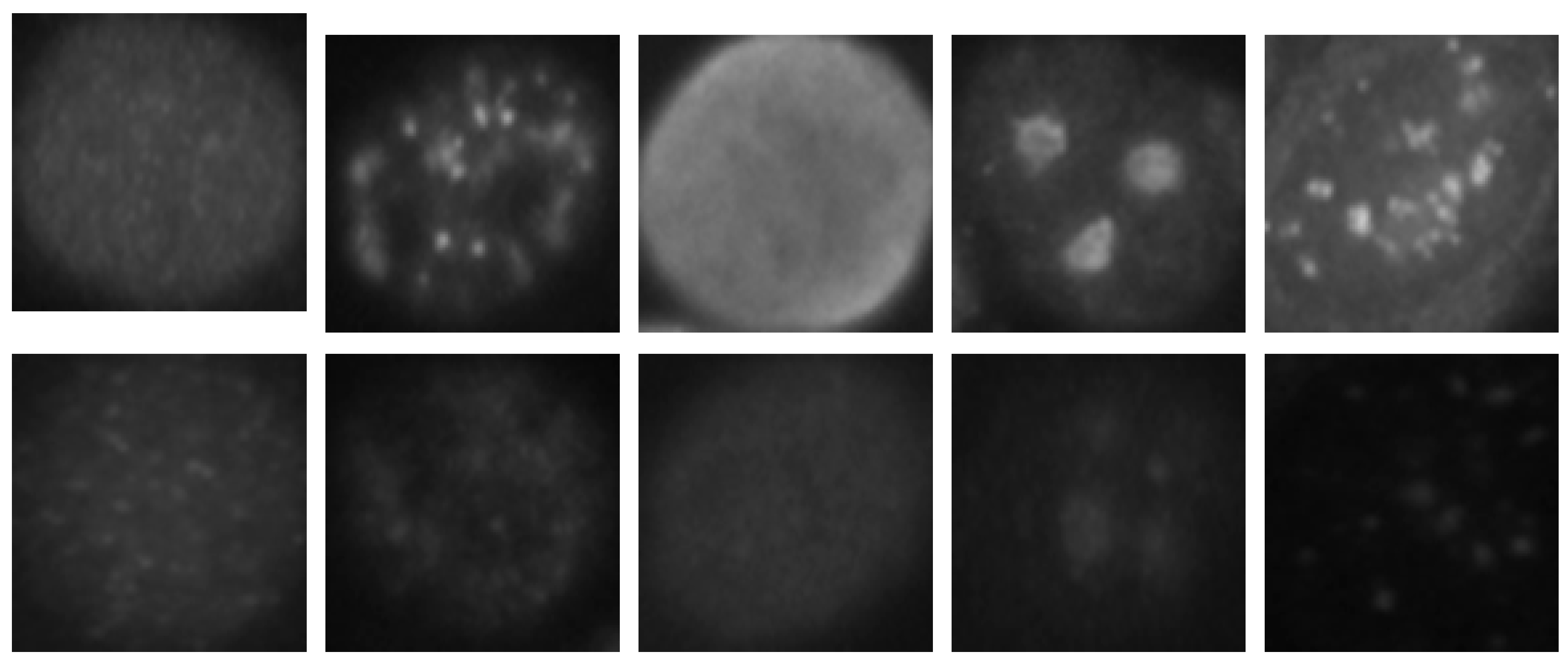
By analyzing the results shown in
Figure 12, we retrieve the problems mostly faced while dealing with the HEp-2 cells’ discrimination: the confusion between the cells that share similarities in terms of the shape and intensity levels. The homogeneous cells are confounded mostly with the fine speckled cells. In
Figure 8, by comparing the two cell types, we can remark that they share a lot of similarities in terms of their shape. If we take a look closely at the fine speckled cells’ classification in
Figure 12, we can notice that the situation is bit worse than for the homogeneous cells. In fact, 8.12% of the fine speckled are classified as homogeneous while “only” 6.42% of the homogeneous are classified as fine speckled. This situation is explained by the fact that most of the negative intensity fine speckled cells, as we can see with the image shown in the second row and third column of
Figure 8, do not show any distinguishable features when we compare them with the homogeneous (both positive and negative intensity) cells. Which means that the disparity related to the fluorescence illumination of the cells encourages the confusion between the cells. The results in
Figure 12 have a total accuracy of 85.64%.
A second observation in
Figure 12 is that the nucleolar cells are quasi-equivalently confounded with the coarse speckled and centromere cells. Even though we can notice the similarity between these three cell types in
Figure 8, this remarkable confusion is also partly attributable to the lack of distinguishability between the negative intensity images of these three cellular types. The results shown in
Figure 12 were obtained without any data augmentation process.
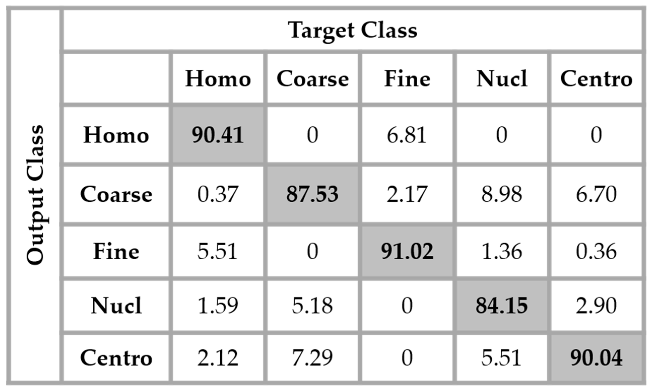
In order to improve the learning capability of the network, data augmentation was applied over the dataset. In every splitting set of the training data, the cells were rotated for 360° with the step of 18°, which is similar with that used in the experiments of Bayramoglu et al. [
29]. Which means that the original training set was expanded by a factor of 20, a 360° quadrant containing 20 portions of 18°. We found that augmenting the training set really improves the accuracy over the testing set. The results shown in
Figure 13 were obtained by using the same network as in
Figure 12 but with data augmentation.
The total accuracy obtained by using data augmentation is 88.63%. Compared to the previous case, where we did not augment the training set, the improvement is around 3%. But, the accuracy still remains low because, as we can notice by analyzing the results shown in
Figure 13, the confusion between the cells that we have previously mentioned still persists. Even though augmenting the training set up to 20 times the original one improves the learning capability of the network, the problem related to the intra-class disparity is not solved at all. The different rotation processes applied over the cells do not decrease the intra-class heterogeneity inherited from the different levels of the fluorescence illumination, the intensity levels of the cells remaining the same even after the rotation.
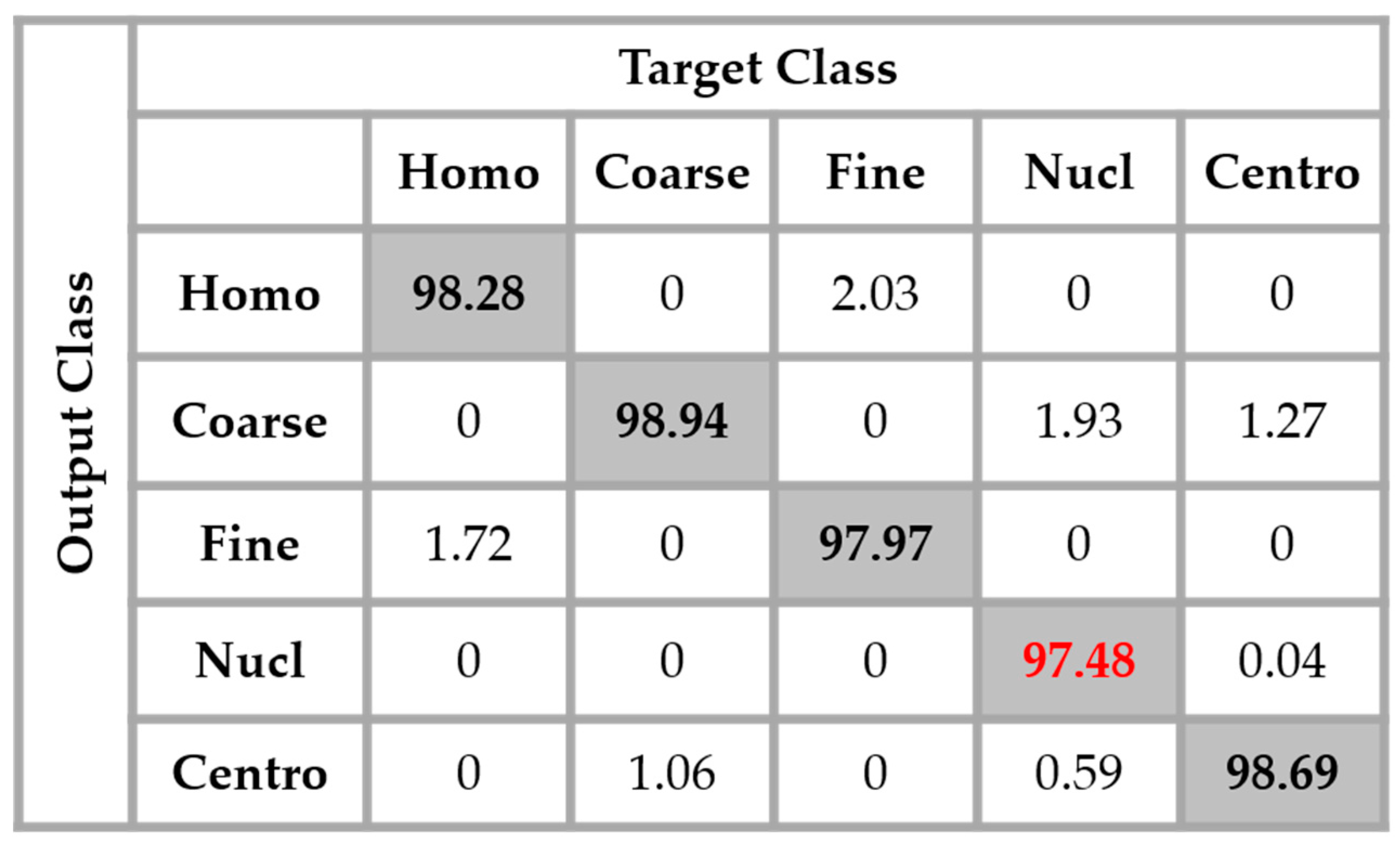
As previously explained in
Section 2, we have used the different DWT coefficients in order to attenuate the intra-class disparity by forcing an intra-class homogenization in terms of the intensity and also the shape. The results obtained by applying the four networks in parallel, as proposed in this work, are shown in the confusion matrix depicted in
Figure 14. These results were obtained without any data augmentation process.
By analyzing
Figure 14, we see that the confusion between the cells has been drastically attenuated. The homogeneous cells are still confounded with the fine speckled cells, but only 2.51% of them were misclassified. On the other hand, the fine speckled cells still pose a complexity problem. But, globally, compared to the previous case, the confusion is really minimized, only 4% of them being classified as homogeneous. This improvement demonstrates the minimization of the intra-class imbalances that has occurred specifically for the fine speckled cells. As explained before, many of the negative intensity fine speckled cells were confounded with both the negative and positive intensity homogeneous cells. However, now we can notice a remarkable homogenization process that allows an improvement of the fine speckled cells’ discrimination.
A second major observation is for the nucleolar cells. As for the previous case, these cells are still quasi-equivalently confounded with the coarse speckled and centromere cells. This cell type stills performs the least compared to the others but an impressive improvement can clearly be observed in the results. In
Figure 14, the result of the nucleolar cells is marked in red. The centromere cells also remain confounded with the coarse speckled cells and also, relatively, with the nucleolar. The total accuracy of the network is 95.30%. Even though we can guess from here that the fact of increasing the learning capability of the networks by applying a huge data augmentation can correct the misclassification cases, we can already notice the remarkable intra-class homogenization that has been achieved by the parallel learning over the dataset. The results obtained when we apply data augmentation are shown in
Figure 15.
By applying data augmentation, the accuracy increases up to 98.27%. The confusion that we have discussed about previously still exists, but in a quite minimal manner. The nucleolar cells still perform the least but, more than 97% of them were well classified. The homogenization in terms of the intensity levels afforded the approximation coefficients, and in terms of the shape, with the different high-frequency components carried by the different details’ coefficients, permit a dynamic learning that minimizes the disparity inherited from the different fluorescence illumination of the cells. The final result is that the global classification is boosted.
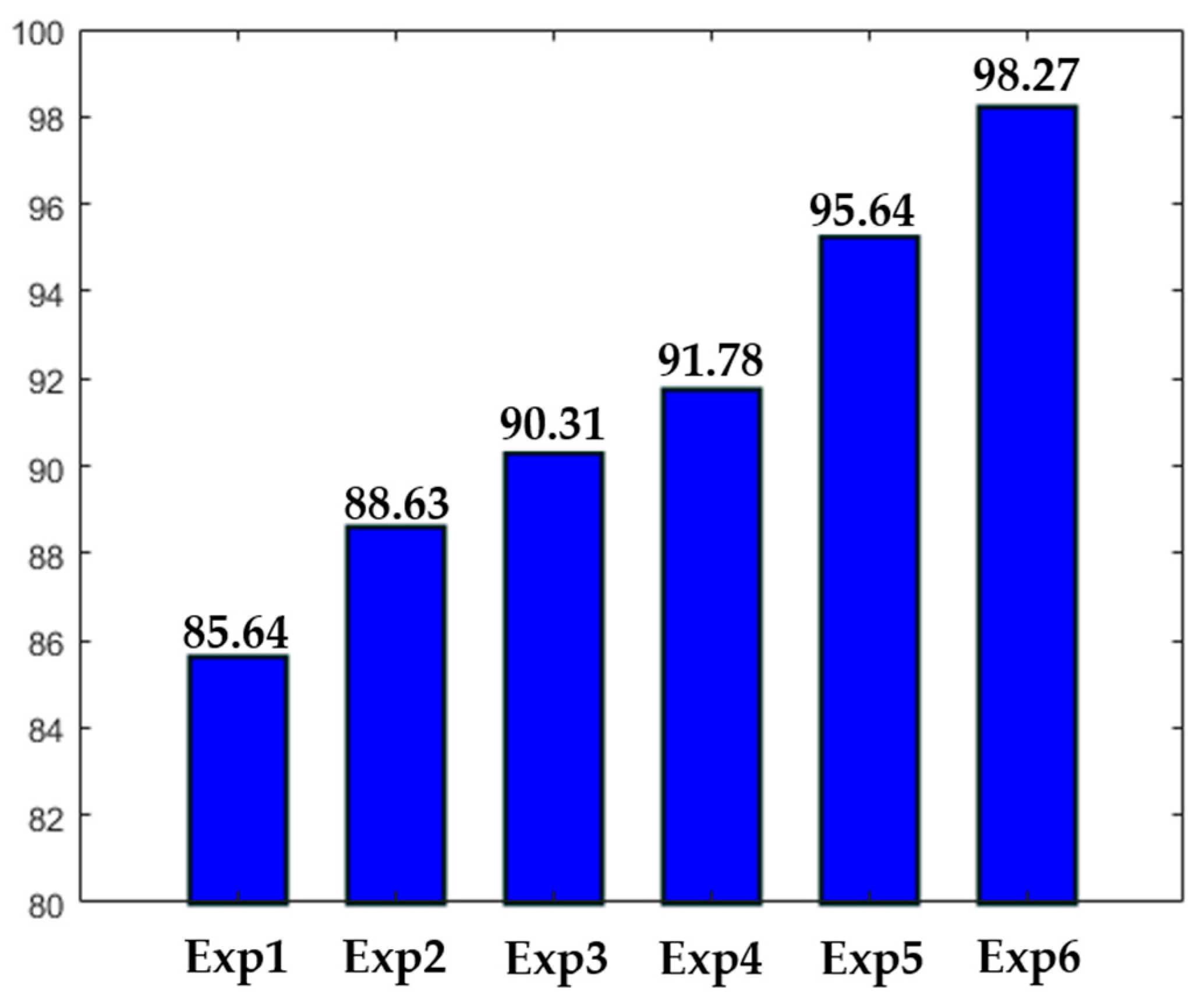
Different experiments were conducted in order to test different hypotheses. The results of the experiments are depicted in
Figure 16. In
Figure 16, “ExpN”, for “Experiment N”, refers to a given experimental scenario. Experiment 1 is the case discussed previously where a single network takes the original images without data augmentation. Experiment 2 is the same scenario with data augmentation applied over the training set, as previously mentioned.
Experiment 3 refers to the case where three networks take only the detail coefficients. In this case, the accuracy is stacked at 90.31%, mainly because the intensity levels between the cells were not homogenized. Experiment 4 refers to the case where only a single network was used. But, in opposite with Experiments 1 and 2, the approximation coefficients were utilized as the inputs, rather than the original images. The accuracy is better than in Experiment 3, but the lack of homogenization in terms of the cellular shape, which is afforded by the detail coefficients, makes the accuracy low. It is necessary to mention that both Experiments 3 and 4 were conducted with data augmentation. Experiments 5 and 6 were discussed previously. The first denotes the case of the four parallel networks without data augmentation, and the latter with data augmentation.
In
Table 1, we show the results of the different methods in the literature. We separate the hand-crafted features-based methods with the ones that utilize deep learning. The texture features [
31], the DCT and SIFT descriptors [
5], and also the LPB descriptors [
6] achieve, respectively, 80.90%, 82.50%, and 85.71%. For all these methods, including the deep learning-based ones discussed in the next paragraph, we have used cross-validation in the same way in order to minimize the biases related to the hyperparameters and the training-testing split.
For the deep learning-based methods, we have also used cross-validation in the same way. Except for our results, where different scenarios (with or without data augmentation) were experimented, all the results shown here for the deep learning-based methods were obtained after applying data augmentation. The state-of-the-art methods proposed in [
23,
27,
28] accomplish 95.61%, 95.99%, and 96.26, respectively, for this highly heterogeneous dataset. Our method clearly boosts the discrimination result on this particular dataset.
We have also tested our method on the most popular ICPR 2016 dataset [
32]. The description of this dataset was discussed previously where we have compared it with the SHPHEp-2 dataset. The hand-crafted features-based methods perform quite poorly on this dataset. It is necessary to mention that for all the deep learning-based methods (only for this dataset, not for the previous one), we just show the results as they were reported by the authors in their works. We have experimented only the hand-crafted features-based methods because all of them were proposed at the time when this dataset was not available. The results are shown in
Table 2.
One thing to notice is that the difference in accuracy between the state-of-the-art methods and our proposed one for the ICPR dataset is not significant. They perform quite similarly. But, as we can see in
Table 1, the difference is a bit more noticeable on the much more heterogeneous and complex dataset, the SNPHEp-2. Also, all of the deep learning-based methods have been proposed especially for the ICPR dataset, which is why all of them provide outstanding results for it.


