A Fast Algorithm for Multi-Class Learning from Label Proportions

Abstract

Learning from label proportions (LLP) is a new kind of learning problem which has attracted wide interest in machine learning. Different from the well-known supervised learning, the training data of LLP is in the form of bags and only the proportion of each class in each bag is available. Actually, many modern applications can be successfully abstracted to this problem such as modeling voting behaviors and spam filtering. However, time-consuming training is still a challenge for LLP, which becomes a bottleneck especially when addressing large bags and bag sizes. In this paper, we propose a fast algorithm called multi-class learning from label proportions by extreme learning machine (LLP-ELM), which takes advantage of an extreme learning machine with fast learning speed to solve multi-class learning from label proportions. Firstly, we reshape the hidden layer output matrix and the training data target matrix of an extreme learning machine to adapt to the proportion information instead of the real labels. Secondly, a robust loss function with a regularization term is formulated and two efficient solutions are provided to different cases. Finally, various experiments demonstrate the significant speed-up of the proposed model with better accuracies on different datasets compared with several state-of-the-art methods.

1. Introduction

In the era of big data, many real-world applications involve a multi-class problem. For example, the MNIST database of handwritten digits is to separate 10 numbers ranging from 0 to 9. Generally speaking, the traditional methods to solve the multi-class problems are adapting supervised learning to learn a multi-class classifier from the training data such as random forests [1], support vector machine [2], convolutional neural networks [3] and boosting [4]. However, many real-world cases fail to be efficiently solved by supervised learning algorithms, which is mainly due to the following two reasons:

On one hand, supervised learning algorithms need large amount of labeled training data in order to obtain a good performance. However, it is becoming infeasible or quite difficulty as the increase of training data. This is because label information is often provided by a human annotator and annotating large datasets is always expensive and time consuming. Furthermore, multiple human annotators often provide inconsistent labels, which could cause the performance of learning algorithms worse. On the other hand, labels of instances are not available in some cases where there are additional constraints. For example, in the client purchasing behaviors analysis [5], we are always prone to adapting supervised learning to learn the clients’ transaction action. However, revealing clients’ key information may cause some legal problems, especially when the information is provided to a third party. This necessitates the development of weakly supervised learning algorithms.

In practice, compared with the accurate labeling individual samples, we can obtain the proportion information of different categories in every bag much more accurately and cheaply by some prior knowledge or random sampling. For example, based on statistics or commonsense, 80% bears are black, 90% Asians are with black hair and 70% living rooms have a TV [6]. Similar problem can be found in gene name tagging, where a word has a 75% probability to be a gene if it ends with the morpheme gene [7]. As a result, it is very meaningful to study the problem of learning from label proportions. Figure 1 illustrates the problem of multi-class learning from class proportions. In detail, there are images of three categories including pandas, butterflies and dolphins and they are divided into four bags with no intersection among them. In each bag, the amount of different categories are denoted by the sizes of rectangles with different colors respectively and a proportion information can be obtained by the sizes of different categories. Then a multi-classifier could be obtained by learning from label proportions. On the right pandas, butterflies and dolphins are separated according to the multi-classifier.

Nowadays, more and more applications can be concluded as this problems, such as demographic classification [8], video event detection [9], presidential election [10], traffic flow prediction [11], embryo implantation prediction [12] and sar image classification [13].

1.1. Related Works

Learning from label proportion has been studied for several years but the papers for the issue are relatively rare. Kuck and de Freitas [14] first gave a solution for this problem, where a Markov Chain Monte Carlo algorithm was employed. However, high computing complexity is a main problem of this algorithm.

Rüping [15] addressed this problem by means of support vector regression. In detail, the mean instance of each bag should comply with a soft label obtained from the label proportion, which use the thought of inverse classifier calibration. Based on the thought, Cui [5] proposed a new algorithm by replacing the SVR by ELM to accelerate the training time. Both of two methods can acquire a relatively good performance. However, Felix X. Yu [16] argued the thought can cause the performance terrible in some cases. Furthermore, both of the two algorithms lack the ability to deal with multi-class problem.

Recently, Felix X. Yu [16] presented a new method based on the large-margin framework. In detail, the objective function was to optimize the known label proportions as well as the unknown instance labels. This model outperforms the former methods in most situations and alleviates the need for making restrictive assumptions on the data. However, the limitations about this method can be further discussed. On one hand, this algorithm cannot handle multi-class problem directly. On the other hand, the training efficiency of this algorithm is very low as it need an alternating process to obtain the following results.

Furthermore, Wang [17] proposed an algorithm based on matrix to directly solve the multi-class classification case, while the others have to perform certain post-processing procedure for multi-class classification. In detail, this method made the predicted class proportions and the ground-truths the same while preserving the sparsity of the predicted label vector of each individual sample. Then a set of auxiliary variables were introduced to solve the optimization problem. Compared to the previous algorithms, the model shows great advantages in handling multi-class problems. However, the algorithm contains matrix computing and it suffers from big computing complexity when the size of instances’ feature goes to considerably big.

Other methods can be found in References [18,19,20,21].

1.2. Motivation

As the amount of data has increased substantially, large-scale and multi-class data has become a trend for many machine learning problems. Generally, large scale data means more time-consuming for training especially for weakly supervised learning where the labels of training data are inaccessible. This necessitates the development of fast learning algorithms for multi-class learning from label proportions. For example, in the case of political election [15], the voters can be divided into three groups: always-favorable voters, always-unsupported voters and swing voters where the last will vote the candidates according to the benefit given to them. Every candidate would like to identify which class each voter belongs to according to proportions information revealed by the previous elections. In particular, the sooner the candidates obtain the information, the higher probability they can take the right action to win the election. This is mainly because they will have more time to focus on their attention to regions where they can achieve the a maximal gain. That is to say, it is a typical LLP problem and a fast solution to it can extremely bring crucial advantage to the candidates.

Although most of the proposed methods have developed effective solutions to LLP [15,16,21,22,23], the time-consuming problem is not fully considered. That is to say, with the increase of bag sizes and bags, they may need unaffordable time to yield a classifier. In order to improve the computational efficiency of the training process, we proposed a fast training method based on ELM which has proven its advantage in fast training speed.

The rest of the paper is organized as follows. First, the extreme learning machine is present in Section 2 and then we show the novel LLP algorithm and the solution to it in Section 3. After this, the experiment results are present in Section 4. Finally, in Section 5, some ideas and conclusions of our work are given.

2. Background

In this section, we give a brief introduction of the traditional extreme learning machine [24,25]. Figure 2 shows the architecture of ELM. In detail, it is a single-hidden layer feed-forward networks with three parts: input neurons, hidden neurons and output neurons. In particular, $\mathbf{h}\left(\mathbf{x}\right)=[h_1\left(x\right),\dots ,h_L\left(x\right)]$ is nonlinear feature mapping of ELM with the form of $h_j\left(x\right)=g({\mathbf{w}}_{\mathbf{j}}.\mathbf{x}+b_j)$ and ${\mathit{\beta }}_{\mathit{j}}={[{\beta }_{j1},...,{\beta }_{jc}]}^T,j=1,\dots ,L$ is the output weights between the jth hidden layer and the output nodes.

Given N samples $(x_i,t_i),i=1,\dots ,N$, where ${\mathbf{x}}_{\mathbf{i}}={[x_{i1},\dots ,x_{id}]}^T$ denotes the input feature vectors and ${\mathbf{t}}_{\mathbf{i}}={[t_{i1},\dots ,t_{ic}]}^T$ is the corresponding label in a one-hot fashion. In particular, c and d respectively represent the total classes and feature number. Consequently, a standard feed-forward neural network with L hidden nodes can be expressed as:

$$\begin{array}{c}\hfill \sum _{j=1}^L{\mathit{\beta }}_{\mathit{j}}g({\mathbf{w}}_{\mathbf{j}}.{\mathbf{x}}_{\mathbf{i}}+b_j)={\mathbf{o}}_{\mathbf{i}},i=1,\dots ,N,\end{array}$$

(1)

where ${\mathbf{w}}_{\mathbf{j}}={[w_{j1},w_{j2},\dots ,w_{jL}]}^T$ is the weight vector between the jth hidden neuron and the input neurons, and ${\mathit{\beta }}_{\mathit{j}}={[{\mathit{\beta }}_{j1},{\mathit{\beta }}_{j2},\dots ,{\mathit{\beta }}_{jc}]}^T,j=1,\dots ,L$ is the weight vector connecting the output neuron and the jth hidden neurons. According to Reference [25], the ELM can approximate those N samples to zero error with the equation ${\sum }_{i=1}^N\parallel {\mathbf{o}}_{\mathbf{i}}-{\mathbf{t}}_{\mathbf{i}}\parallel =0$. Thus, the above equations can be expressed as:

$$\begin{array}{c}\hfill \sum _{j=1}^L{\mathit{\beta }}_{\mathit{j}}g({\mathbf{w}}_{\mathbf{j}}.{\mathbf{x}}_{\mathbf{i}}+b_j)={\mathbf{t}}_{\mathbf{i}},i=1,\dots ,N.\end{array}$$

(2)

In particular, we can use matrix to express the above N equations with form of:

$$\begin{array}{c}\hfill \mathbf{H}\mathit{\beta }=\mathbf{T},\end{array}$$

(3)

where H is the hidden layer output matrix of the single-hidden layer feed-forward network and T is output matrix. More specifically, H and T have the form of:

$$\mathbf{H}=\left[\begin{array}{c}\mathbf{h}\left({\mathbf{x}}_{\mathbf{1}}\right)\\ ⋮\\ \mathbf{h}\left({\mathbf{x}}_{\mathbf{N}}\right)\end{array}\right]=\left[\begin{array}{ccc}{h}_1\left({\mathbf{x}}_{\mathbf{1}}\right)& \cdots & h_L\left({\mathbf{x}}_{\mathbf{1}}\right)\\ ⋮& ⋮& ⋮\\ h_1\left({\mathbf{x}}_{\mathbf{N}}\right)& ⋮& h_L\left({\mathbf{x}}_{\mathbf{N}}\right)\end{array}\right]$$

(4)

and

$$\mathbf{T}=\left[\begin{array}{c}{\mathbf{t}}_{\mathbf{1}}^{\mathbf{T}}\\ ⋮\\ {\mathbf{t}}_{\mathbf{N}}^{\mathbf{T}}\end{array}\right]=\left[\begin{array}{ccc}{t}_{11}& \cdots & t_{1c}\\ ⋮& ⋮& ⋮\\ t_{N1}& ⋮& t_{Nc}\end{array}\right].$$

(5)

In practice, the hidden node parameters (w,b) of ELM are randomly generated and then fixed without iteratively tuning, which is different to the traditional BP neural networks [25]. As a result, training an ELM is equivalent to find the optimal solution to $\mathit{\beta }$, which is in defined as:

$$\mathit{\beta }=\left[\begin{array}{c}{\mathit{\beta }}_{\mathbf{1}}^{\mathit{T}}\\ ⋮\\ {\mathit{\beta }}_{\mathit{L}}^{\mathit{T}}\end{array}\right]=\left[\begin{array}{ccc}{\beta }_{11}& \cdots & {\beta }_{1c}\\ ⋮& ⋮& ⋮\\ {\beta }_{L1}& ⋮& {\beta }_{Lc}\end{array}\right].$$

(6)

Furthermore, $\mathit{\beta }$ can be computed by the following expression:

$${\mathit{\beta }}^{*}={\mathbf{H}}^{†}\mathbf{T},$$

(7)

where ${\mathbf{H}}^{†}$ is the Moore-Penrose generalized inverse of matrix H.

3. The LLP-ELM Algorithm

In this section, we propose a fast method for multi-class learning from label proportions algorithm called LLP-ELM, which employs an extreme learning machine to solve multi-class LLP problem. In order to leverage the extreme learning machine to LLP, we reshape the hidden layer output matrix H and the training data target matrix T to new forms, such that H is in bag level and T contains the proportion information instead of a label one.

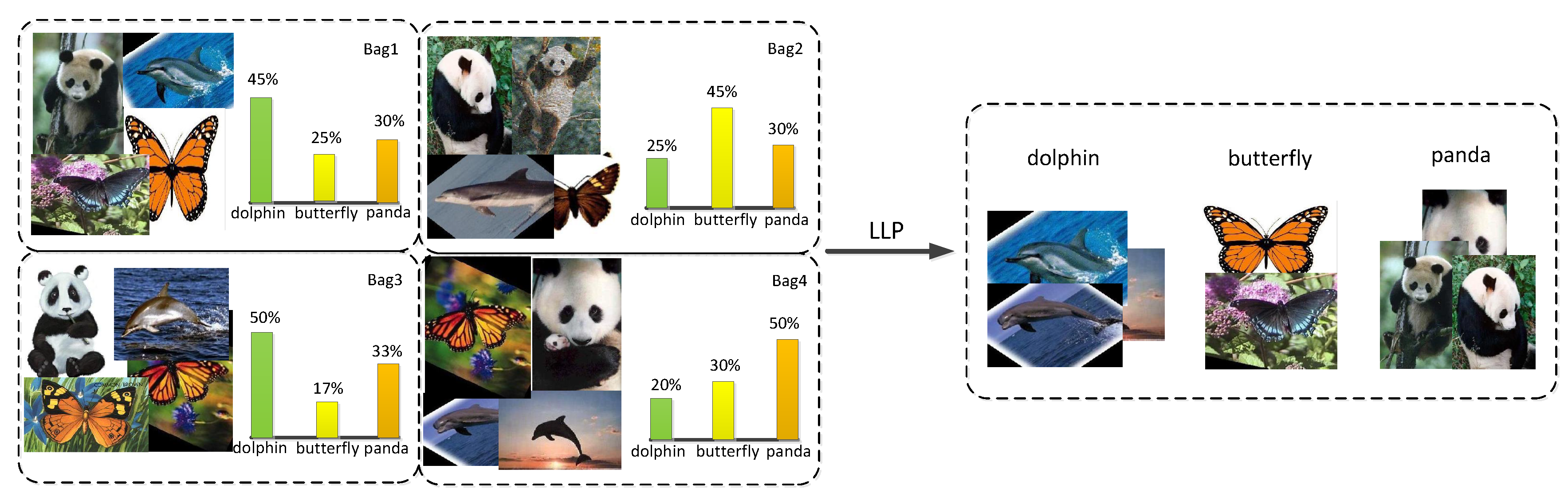
3.1. Learning Setting

The LLP problem is described by a set of training data, which is divided into several bags. Furthermore, compared to the traditional supervised learning, we only know the proportions of different categories in each bag instead of the ground-truth labels. In this paper, we consider the situation that different bags are disjoint and the nth bag of the training data can be denoted as $B_n,n=1,\dots ,h$. Consequently, the total training data is in form of:

$$\begin{array}{c}\hfill D=B_1\cup B_2\cup \dots \cup B_h\\ \hfill B_i\cap B_j=\varnothing ,\forall i\ne j.\end{array}$$

(8)

where there are n bags and N is the number of total instances. Each bag consists of $m_n$ instances with the constraint ${\sum }_{n=1}^h{m}_n=N$ and can be expressed as:

$$\begin{array}{c}\hfill B_n=\{x_n^1,\dots ,x_n^{m_n}\},n\in \{1,2,\dots ,h\}.\end{array}$$

(9)

Meanwhile, ${\mathbf{p}}_{\mathbf{n}}$ is the corresponding class proportion vector of $B_n$ and c represents the total classes number. More specifically, ${\mathbf{p}}_{\mathbf{n}}$ can be written as a vector form:

$${\mathbf{p}}_{\mathbf{n}}=\left[\begin{array}{c}{p}_{n1}\\ ⋮\\ p_{nc}\end{array}\right],$$

(10)

where the mth element $p_n^m$ is the proportion of the mth class in the nth bag with the constraint ${\sum }_{m=1}^c{p}_n^m=1$. Furthermore, the total proportion information can be defined in form of matrix:

$$\mathbf{P}=\left[\begin{array}{c}{\mathbf{p}}_{\mathbf{1}}^{\mathbf{T}}\\ ⋮\\ {\mathbf{p}}_{\mathbf{h}}^{\mathbf{T}}\end{array}\right]=\left[\begin{array}{ccc}{p}_{11}& \cdots & p_{1c}\\ ⋮& ⋮& ⋮\\ p_{h1}& ⋮& p_{hc}\end{array}\right].$$

(11)

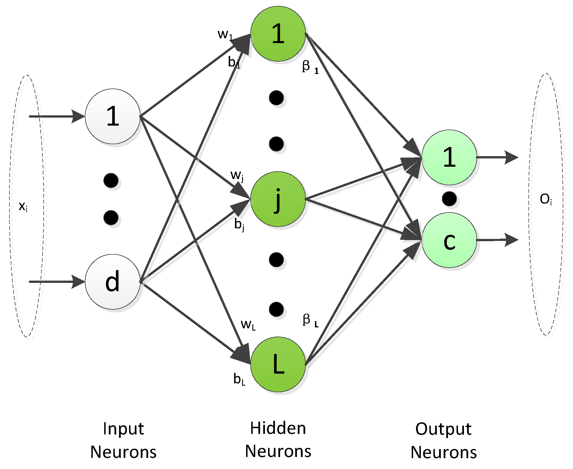
3.2. The LLP-ELM Framework

From the above learning setting of LLP, a classifier in instance level is the final objective. To this end, we modify the original equations in ELM to the new equations in bag level. Specifically, we add all the equations in each bag straightforward and the final equations in nth bag can be expressed as follows:

$$\begin{array}{c}\hfill \sum _{j=1}^L\sum _{k=1}^{m_n}{\mathit{\beta }}_{\mathit{j}}g({\mathbf{w}}_{\mathbf{j}}.{\mathbf{x}}_{\mathbf{nk}}+b_j)=\sum _{k=1}^{m_n}{\mathbf{t}}_{\mathbf{nk}},n=1,\dots ,h,\end{array}$$

(12)

where ${\mathbf{t}}_{\mathbf{nk}}$ is the real label for the kth instances in nth bag. Obviously, the real label information in the right part is inaccessible to us, with only label proportions in each bag available. To this end, we derive the right part of the above equation as the following form:

$$\begin{array}{c}\hfill \sum _{k=1}^{m_n}{\mathbf{t}}_{\mathbf{nk}}=m_n\ast {\mathbf{p}}_{\mathbf{n}},n=1,\dots ,h,\end{array}$$

(13)

where ${\mathbf{p}}_{\mathbf{n}}$ is the label proportion of nth bag. Substituting the formula (13) to (12), we can naturally obtain the following equations:

$$\begin{array}{c}\hfill \sum _{j=1}^L{\mathit{\beta }}_{\mathit{j}}\sum _{k=1}^{m_n}g({\mathbf{w}}_{\mathbf{j}}.{\mathbf{x}}_{\mathbf{nk}}+b_j)=m_n\ast {\mathbf{p}}_{\mathbf{j}},n=1,\dots ,h,\end{array}$$

(14)

In particular, similar to the method from ELM [25], we can write the above equations in the form of matrix computing as follows:

$$\begin{array}{c}\hfill {\mathbf{H}}_{\mathbf{p}}\mathit{\beta }=\mathbf{P},\end{array}$$

(15)

where ${\mathbf{H}}_{\mathbf{p}}$ is the hidden layer output matrix in the bag level and $\mathbf{P}$ is the training data target proportion matrix. More specifically, ${\mathbf{H}}_{\mathbf{p}}$ and $\mathbf{P}$ are given in form of:

$${\mathbf{H}}_{\mathbf{p}}=\left[\begin{array}{c}{\displaystyle \sum _{k=1}^{m_1}}\mathbf{h}\left({\mathbf{x}}_{\mathbf{1}\mathbf{k}}\right)\\ ⋮\\ {\displaystyle \sum _{k=1}^{m_h}}\mathbf{h}\left({\mathbf{x}}_{\mathbf{hk}}\right)\end{array}\right]=\left[\begin{array}{ccc}{\displaystyle \sum _{k=1}^{m_1}}{h}_1\left({\mathbf{x}}_{\mathbf{1}\mathbf{k}}\right)& \cdots & {\displaystyle \sum _{k=1}^{m_1}}{h}_L\left({\mathbf{x}}_{\mathbf{1}\mathbf{k}}\right)\\ ⋮& ⋮& ⋮\\ {\displaystyle \sum _{k=1}^{m_h}}{h}_1\left({\mathbf{x}}_{\mathbf{hk}}\right)& ⋮& {\displaystyle \sum _{k=1}^{m_h}}{h}_L\left({\mathbf{x}}_{\mathbf{hk}}\right)\end{array}\right]$$

and

$$\mathbf{P}=\left[\begin{array}{c}{m}_1\ast {\mathbf{p}}_{\mathbf{1}}^{\mathbf{T}}\\ ⋮\\ m_h\ast {\mathbf{p}}_{\mathbf{h}}^{\mathbf{T}}\end{array}\right]=\left[\begin{array}{ccc}{m}_1\ast p_{11}& \cdots & m_1\ast p_{1c}\\ ⋮& ⋮& ⋮\\ m_h\ast p_{h1}& ⋮& m_h\ast p_{hc}\end{array}\right].$$

Meanwhile, the final solution $\mathit{\beta }$ is the same with the original form in ELM with dimension $L\times c$. Again, the optimal solution to (15) is given by

$$\begin{array}{c}\hfill {\mathit{\beta }}^{\ast }={\mathbf{H}}_{\mathbf{p}}^{†}\mathbf{P},\end{array}$$

(16)

where ${\mathbf{H}}_{\mathbf{p}}^{†}$ is the Moore-Penrose generalized by the inverse of matrix ${\mathbf{H}}_{\mathbf{p}}$.

In order to obtain a better generalization performance of ELM, we also follow the method from Reference [24] to study the regularized ELM. In detail, the final objective function of ELM is formulated as follows:

$$\begin{array}{c}\underset{\mathit{\beta }\in R^{L\times c}}{min}\frac{1}{2}{\parallel \mathit{\beta }\parallel }^2+\frac{C}{2}{\displaystyle \sum _{i=1}^N}{\parallel {\mathbf{e}}_{\mathbf{i}}\parallel }^2\hfill \\ s.t.\mathbf{h}\left({\mathbf{x}}_{\mathbf{i}}\right)\mathit{\beta }={\mathbf{t}}_{\mathbf{i}}^{\mathbf{T}}-{\mathbf{e}}_{\mathbf{i}}^{\mathbf{T}},i=1,\dots ,N,\hfill \end{array}$$

(17)

in which the first term of the objective function is a regularization term and C is a parameter to make a trade-off between the first and second term.

We equivalently reformulate the problem (17) as follows by substituting the constraints to its objective function:

$$\begin{array}{c}\hfill \underset{\mathit{\beta }\in R^{L\times c}}{min}{L}_{ELM}=\frac{1}{2}{\parallel \mathit{\beta }\parallel }^2+\frac{C}{2}{\parallel \mathbf{T}-\mathbf{H}\mathit{\beta }\parallel }^2.\end{array}$$

(18)

Note that the second term of (18) can be replaced by $\frac{C}{2}{\parallel \mathbf{P}-{\mathbf{H}}_{\mathbf{p}}\mathit{\beta }\parallel }^2$, which is the matrix form in bag level. In other words, the final unconstrained optimization problem can be written as:

$$\begin{array}{c}\hfill \underset{\mathit{\beta }\in R^{L\times c}}{min}{L}_{ELM}=\frac{1}{2}{\parallel \mathit{\beta }\parallel }^2+\frac{C}{2}{\parallel \mathbf{P}-{\mathbf{H}}_{\mathbf{p}}\mathit{\beta }\parallel }^2.\end{array}$$

(19)

In practice, the final objection is widely known as the ridge regression or regularized least squares.

3.3. How to Solve the LLP-ELM

We follow the strategy from Reference [24] to solve (19) and the final purpose is to minimize the training error as well as the norm of the output weights. Obviously, the final objective function is a convex problem, which is always solved by way of gradient. More specifically, by setting the gradient of (19) to zero with respect to $\mathit{\beta }$, we can obtain the following expression:

$$\begin{array}{c}\hfill \mathit{\beta }-C{\mathbf{H}}_{\mathbf{p}}^{\mathbf{T}}(\mathbf{P}-{\mathbf{H}}_{\mathbf{p}}\mathit{\beta })=\mathbf{0}.\end{array}$$

(20)

This yields

$$\begin{array}{c}\hfill (\frac{\mathbf{I}}{\mathbf{C}}+{\mathbf{H}}_{\mathbf{p}}^{\mathbf{T}}{\mathbf{H}}_{\mathbf{p}})\mathit{\beta }={\mathbf{H}}_{\mathbf{p}}^{\mathbf{T}}\mathbf{P},\end{array}$$

(21)

where $\mathbf{I}$ is an identity matrix with dimension L.

The above equation is very intuitive and we can obtain the final optimization result by inverting a L × L matrix directly. However, it is less efficient to directly invert a L × L matrix when the number of bag is less than the number of hidden neurons (h < L). Therefore, there are two methods which are shown in Remarks 1 and 2. In summary, in the case where the number of bags are plentiful than hidden neurons, we use Remark 1 to compute the output weights, otherwise we use Remark 2.

Remark 1.

The solution for Formula (20) when h > L.

• ${\mathbf{H}}_{\mathbf{p}}$ has more rows than columns, which means the number of bag is larger than the number of hidden neurons.
• By inverting a L×L matrix directly and multiplying both sides by ${({\mathbf{H}}_{\mathbf{p}}^{\mathbf{T}}{\mathbf{H}}_{\mathbf{p}}+\frac{\mathbf{I}}{\mathbf{C}})}^{-\mathbf{1}}$, we can obtain the following expression

  $$\begin{array}{c}\hfill \mathit{\beta }={({\mathbf{H}}_{\mathbf{p}}^{\mathbf{T}}{\mathbf{H}}_{\mathbf{p}}+\frac{\mathbf{I}}{\mathbf{C}})}^{-\mathbf{1}}{\mathbf{H}}_{\mathbf{p}}^{\mathbf{T}}\mathbf{P},\end{array}$$

  (22)

  which is the optimal solution of (20).

Remark 2.

The solution for formula (20) when h < L.

• Notice that ${\mathbf{H}}_{\mathbf{p}}$ is full row rank and ${\mathbf{H}}_{\mathbf{p}}{\mathbf{H}}_{\mathbf{p}}^{\mathbf{T}}$ is invertible when h < L.
• Restrict β to be a linear combination of the row in ${\mathbf{H}}_{\mathbf{p}}:\mathit{\beta }={\mathbf{H}}_{\mathbf{p}}^{\mathbf{T}}\alpha$
• Substitute $\mathit{\beta }={\mathbf{H}}_{\mathbf{p}}^{\mathbf{T}}\mathit{\alpha }$ into (20) and multiply by ${\left({\mathbf{H}}_{\mathbf{p}}{\mathbf{H}}_{\mathbf{p}}^{\mathbf{T}}\right)}^{-\mathbf{1}}{\mathbf{H}}_{\mathbf{p}}$.
• By the above step, we can obtain the following equation:

  $$\begin{array}{c}\hfill \mathit{\alpha }-C(\mathbf{P}-{\mathbf{H}}_{\mathbf{p}}{\mathbf{H}}_{\mathbf{p}}^{\mathbf{T}}\mathit{\alpha })=\mathbf{0}.\end{array}$$

  (23)
• As a result, the final optimal solution of (20) is in form of

  $$\begin{array}{c}\hfill \mathit{\beta }={\mathbf{H}}_{\mathbf{p}}^{\mathbf{T}}\mathit{\alpha }={\mathbf{H}}_{\mathbf{p}}^{\mathbf{T}}{({\mathbf{H}}_{\mathbf{p}}{\mathbf{H}}_{\mathbf{p}}^{\mathbf{T}}+\frac{\mathbf{I}}{\mathbf{C}})}^{-\mathbf{1}}\mathbf{P}=\mathbf{0}.\end{array}$$

  (24)

The solution process of LLP-ELM model can be concluded to the following two steps:

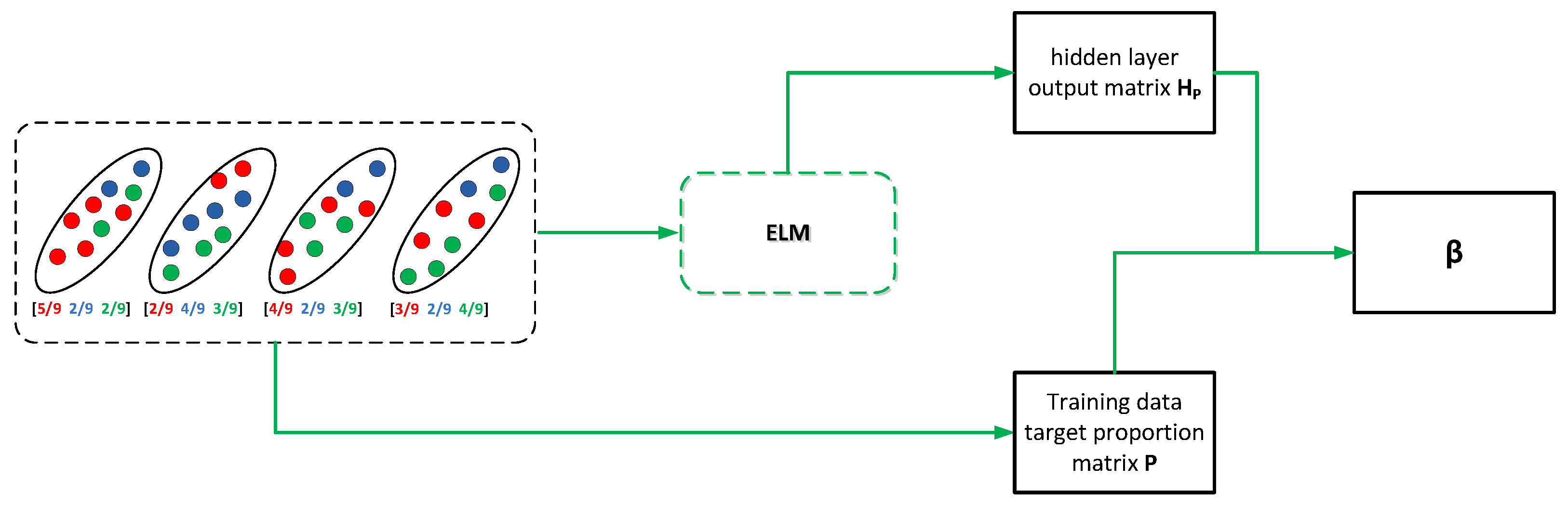
• Compute training data target proportion matrix $\mathbf{P}$ and the hidden layer output matrix ${\mathbf{H}}_{\mathbf{p}}$, which is shown in Figure 3.
• Obtain the final optional solution of $\mathit{\beta }$ according to Remark 1 or Remark 2.

The details of the process are shown in Algorithm 1.

Algorithm 1 LLP-ELM

Input: Training datasets in bags$\left\{B_n\right\}$; The corresponding proportion $p_n$ of $B_n$; Activation function g(x) and the number of hidden nodes N.  Output: Classification model f(x,$\mathit{\beta }$)  Begin  • Randomly initialize the value ${\mathbf{w}}_{\mathbf{j}}$ and $b_j$ for the jth node, $j=1,\dots ,L.$  • Compute the training data target proportion matrix $\mathbf{P}$ by the proportion information of each bag.  • Compute the hidden layer output matrix in the bag level ${\mathbf{H}}_{\mathbf{p}}$.  • Obtain the weight vector according to Remark 1 or Remark 2.  End

3.4. Computational Complexity

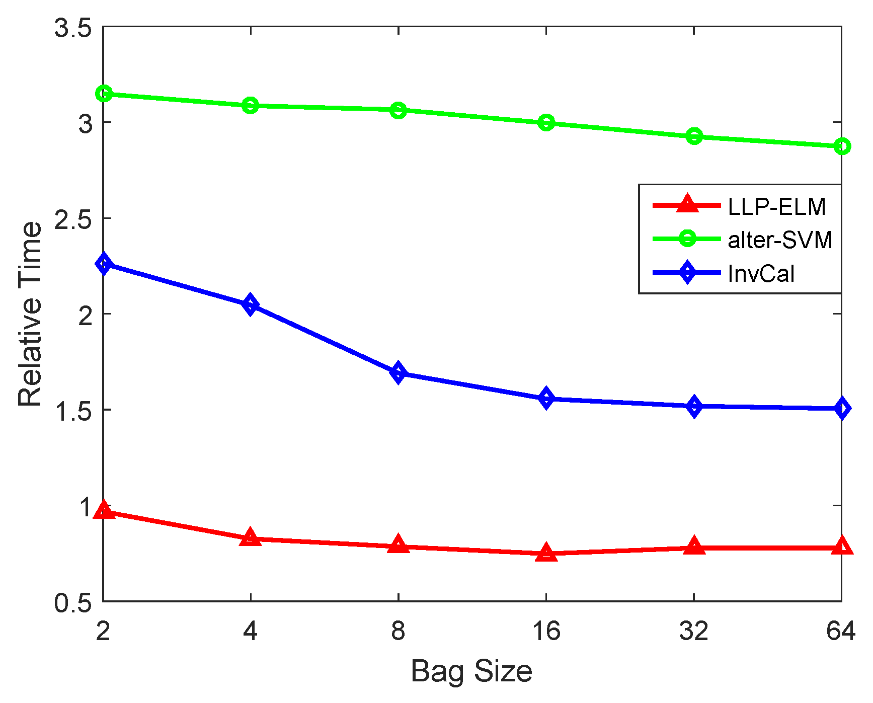
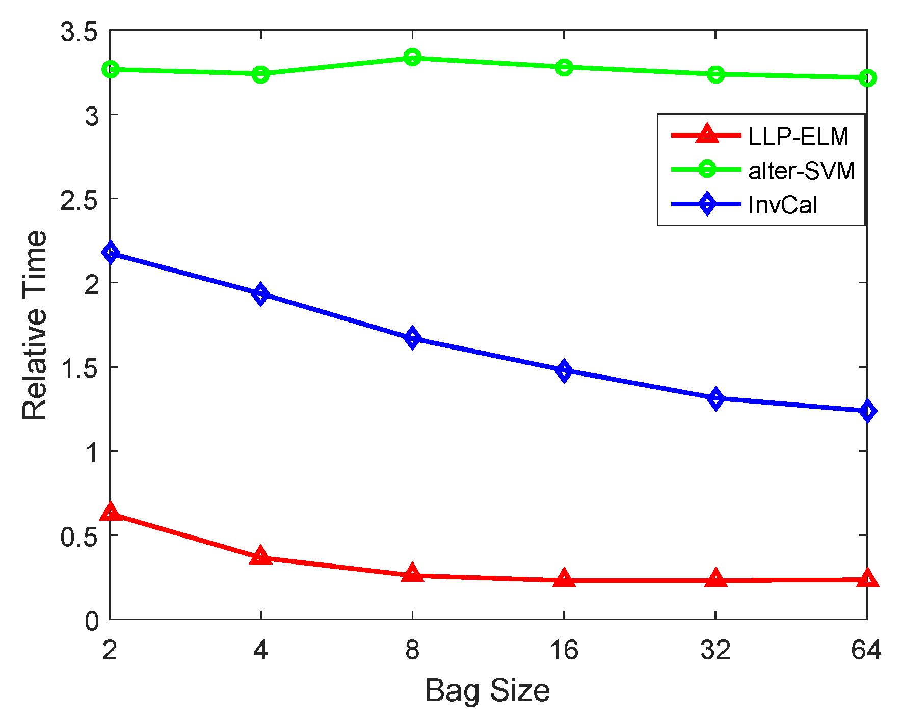
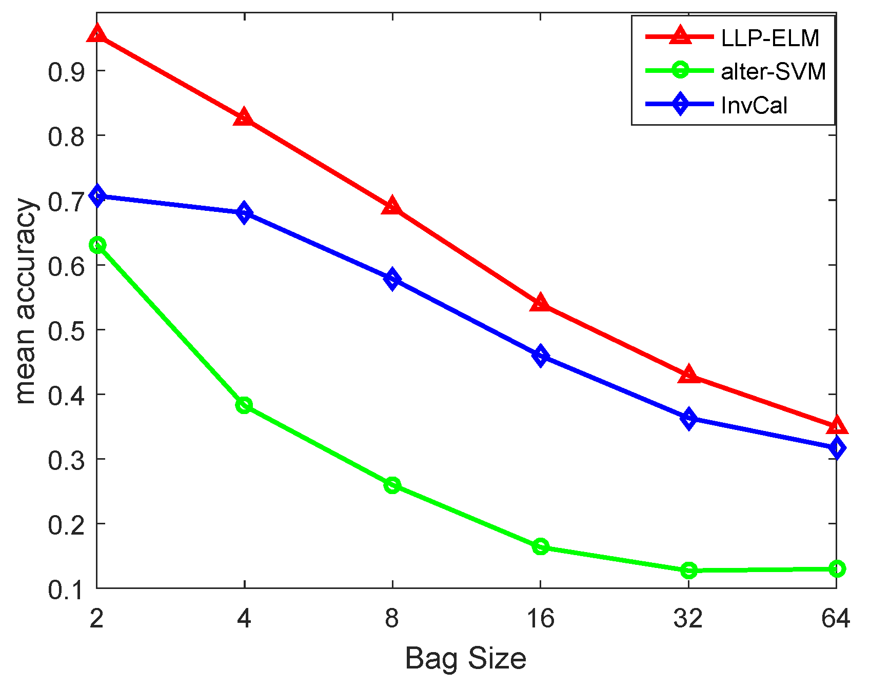
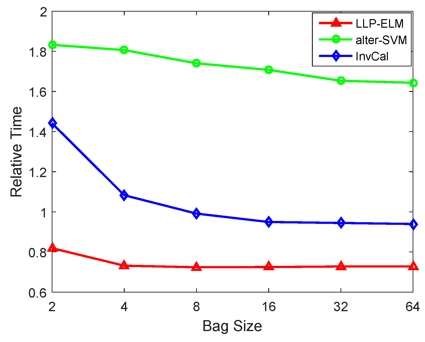
From the Remarks 1 and 2, we can observe that the main time cost of our method is to calculate the matrix inversion. Furthermore, the dimension of matrix is minimum of the number of bags h and the hidden neurons L, which is determined by us. As we all know, the complexity of matrix inversion is proportional to the $O^3$, where O is the dimension of matrix and is equal to Min(L,h) in this paper.

4. Experiments

In this section, we evaluate the performance of our proposed algorithm on binary and multi-class datasets and two methods from References [15,16] are used to compare with our model. The two methods have proven their advantage compared to previous methods. Additional, the training time of the three algorithms on different datasets is presented. Our source code is available on https://github.com/liujiabin008/LLP-ELM-GITHUB.

4.1. Experiment Setting

The total data is partitioned into two parts: 80% for training data and 20% for testing. Furthermore, we random split the training data into different bags with bag sizes 2, 4, 8, 16, 32 and 64. The final results contain training time and classification accuracy by repeating the experiment 5 times.

For alter-∝SVM, we need to give an initial value to the labels and in practice a stochastic method is employed according to the proportions information of different bags. Furthermore, alter-∝SVM need to run several times to reduce the influence of random initialization, with choosing the lowest objective value as the final result.

In particular, the attributes are scaled to [−1;1] for each dataset and 3000 neurons in hidden layer are used in the experiment for LLP-ELM. Furthermore, linear kernel is considered for alter-∝SVM and InvCal in our experiments. All the parameters are tuned in the criterion of fivefold cross validation. In detail, the parameters of different algorithms are tuned as follows:

$$\begin{array}{cc}\hfill InvCal:& C_p\in [0.1,1,10],\epsilon \in [0,0.1,0.01]\hfill \\ \hfill alter-\propto SVM:& C\in [0.1,1,10],C_p\in [1,10,100]\hfill \\ \hfill LLP-ELM:& C\in [0.1,1,0.01]\hfill \end{array}$$

4.2. Binary Datasets

In this section, we compare our algorithm with two state-of-art methods called alter-∝SVM [16] and InvCal [15] on 9 binary classification problems.

Table 1. Binary datasets in the experiment.

Dataset	Size	Attributes
sonar	208	60
heart	270	13
vote	435	16
breast-cancer	683	10
credit-a	690	15
diabetes	768	8
pima-indian	768	8
splice	1000	60
ala	1065	119

is the summary of the 9 datasets with size and attributes, where the size of different datasets is bigger from up to down.

The final performance of the three algorithms is presented in

Table 2. The final results under the optimal parameters with bag size 2, 4, 8, 16, 32, 64. Bold numbers denote the best accuracies.

Dataset	Method	2	4	8	16	32	64
	InvCal	0.76 ± 0.12	0.70 ± 0.11	0.72 ± 0.11	0.65 ± 0.14	0.59 ± 0.12	0.50 ± 0.13
sonar	alter-∝SVM	0.74 ± 0.09	0.64 ± 0.09	0.51 ± 0.11	0.595 ± 0.06	0.53 ± 0.10	0.49 ± 0.13
	LLP-ELM	0.91 ± 0.02	0.78 ± 0.03	0.74 ± 0.04	0.68 ± 0.09	0.58 ± 0.04	0.55 ± 0.07
	InvCal	0.80 ± 0.05	0.79 ± 0.04	0.81 ± 0.06	0.71 ± 0.11	0.75 ± 0.07	0.73 ± 0.14
heart	alter-∝SVM	0.81 ± 0.04	0.79 ± 0.03	0.80 ± 0.03	0.78 ± 0.11	0.66 ± 0.20	0.77 ± 0.07
	LLP-ELM	0.88 ± 0.02	0.84 ± 0.02	0.78 ± 0.03	0.75 ± 0.11	0.76 ± 0.04	0.74 ± 0.09
	InvCal	0.95 ± 0.03	0.94 ± 0.03	0.94 ± 0.04	0.92 ± 0.02	0.89 ± 0.04	0.84 ± 0.07
vote	alter-∝SVM	0.95 ± 0.01	0.94 ± 0.03	0.94 ± 0.02	0.95 ± 0.01	0.91 ± 0.06	0.89 ± 0.01
	LLP-ELM	0.98 ± 0.01	0.97 ± 0.01	0.96 ± 0.01	0.95 ± 0.01	0.91 ± 0.01	0.90 ± 0.05
	InvCal	0.95 ± 0.01	0.94 ± 0.01	0.95 ± 0.02	0.95 ± 0.03	0.95 ± 0.01	0.90 ± 0.05
breast-cancer	alter-∝SVM	0.96 ± 0.02	0.96 ± 0.01	0.96 ± 0.02	0.96 ± 0.02	0.96 ± 0.01	0.97 ± 0.01
	LLP-ELM	0.97 ± 0.00	0.97 ± 0.00	0.97 ± 0.00	0.96 ± 0.01	0.93 ± 0.02	0.92 ± 0.04
	InvCal	0.85 ± 0.02	0.85 ± 0.02	0.85 ± 0.03	0.82 ± 0.02	0.82 ± 0.03	0.77 ± 0.09
credit-a	alter-∝SVM	0.85 ± 0.02	0.85 ± 0.02	0.81 ± 0.05	0.82 ± 0.02	0.64 ± 0.14	0.76 ± 0.08
	LLP-ELM	0.89 ± 0.01	0.88 ± 0.02	0.83 ± 0.02	0.80 ± 0.03	0.74 ± 0.08	0.76 ± 0.06
	InvCal	0.75 ± 0.03	0.71 ± 0.05	0.73 ± 0.04	0.67 ± 0.05	0.66 ± 0.05	0.64 ± 0.03
diabetes	alter-∝SVM	0.76 ± 0.02	0.73 ± 0.03	0.71 ± 0.04	0.67 ± 0.03	0.66 ± 0.04	0.66 ± 0.05
	LLP-ELM	0.78 ± 0.01	0.78 ± 0.02	0.75 ± 0.01	0.72 ± 0.02	0.67 ± 0.02	0.68 ± 0.02
	InvCal	0.76 ± 0.03	0.70 ± 0.05	0.72 ± 0.04	0.70 ± 0.06	0.66 ± 0.07	0.65 ± 0.03
pima-indian	alter-∝SVM	0.75 ± 0.03	0.73 ± 0.03	0.70 ± 0.03	0.67 ± 0.04	0.66 ± 0.03	0.65 ± 0.02
	LLP-ELM	0.78 ± 0.00	0.77 ± 0.01	0.75 ± 0.01	0.73 ± 0.01	0.71 ± 0.03	0.56 ± 0.07
	InvCal	0.79 ± 0.02	0.73 ± 0.02	0.73 ± 0.06	0.65 ± 0.03	0.63 ± 0.05	0.60 ± 0.04
splice-scale	alter-∝SVM	0.78 ± 0.04	0.74 ± 0.03	0.71 ± 0.04	0.65 ± 0.05	0.66 ± 0.04	0.56 ± 0.17
	LLP-ELM	0.94 ± 0.01	0.82 ± 0.03	0.78 ± 0.02	0.69 ± 0.03	0.65 ± 0.03	0.60 ± 0.05
	InvCal	0.82 ± 0.02	0.78 ± 0.03	0.77 ± 0.02	0.71 ± 0.05	0.74 ± 0.03	0.71 ± 0.05
ala	alter-∝SVM	0.82 ± 0.02	0.79 ± 0.04	0.79 ± 0.03	0.72 ± 0.06	0.76 ± 0.02	0.75 ± 0.02
	LLP-ELM	0.9 ± 0.00	0.85 ± 0.01	0.81 ± 0.01	0.76 ± 0.02	0.76 ± 0.02	0.75 ± 0.03

, where the 9 datasets are arranged in order of increasing size and the bold numbers means the best accuracy in the special dataset.

As can be seen from this table, our method always has a higher accuracy than InvCal and alter-∝SVM on most datasets, with acquiring 40 best, 9 second and 5 last from the total 54 results. Especially on the datasets of diabetes and ala, LLP-ELM is superior to the other two algorithms in all bag sizes. In particular, we can obtain that as the increase of bag size, the accuracy of the three methods decrease in different degrees. This is mainly because less information is provided as the increase of bag size.

Additionally, the average classification accuracies on the 9 datasets are shown in Figure 4 with different bag size. In detail, alter-∝SVM, InvCal and ELM-LLP are respectively denoted by green, blue and red lines. From the results, we can clearly see that our method is superior to the other two algorithms in classification accuracy.

We also present the training time of different methods in

Table 3. Training time (second) of different algorithms with bag size 2, 4, 8, 16, 32 and 64. Bold numbers denote the least training time.

Dataset	Method	2	4	8	16	32	64
	InvCal	0.83	0.38	0.35	0.33	0.32	0.31
sonar	alter-∝SVM	1.66	1.19	0.68	0.53	0.42	0.37
	LLP-ELM	0.03	0.02	0.02	0.02	0.02	0.02
	InvCal	0.50	0.40	0.33	0.33	0.32	0.31
heart	alter-∝SVM	2.16	1.51	1.01	0.78	0.67	0.61
	LLP-ELM	0.03	0.02	0.02	0.02	0.02	0.02
	InvCal	0.61	0.46	0.35	0.33	0.32	0.31
vote	alter-∝SVM	3.83	2.82	2.88	2.14	1.73	1.54
	LLP-ELM	0.05	0.04	0.04	0.04	0.04	0.03
	InvCal	1.46	0.58	0.41	0.35	0.32	0.31
breast-cancer	alter-∝SVM	7.82	5.71	5.25	4.95	4.05	4.02
	LLP-ELM	0.08	0.06	0.05	0.05	0.05	0.05
	InvCal	1.64	1.61	0.43	0.35	0.34	0.32
credit-a	alter-∝SVM	9.39	7.35	6.84	6.07	5.32	4.95
	LLP-ELM	0.08	0.06	0.06	0.05	0.06	0.06
	InvCal	1.90	0.63	0.43	0.35	0.33	0.31
diabetes	alter-∝SVM	13.32	11.19	9.24	8.05	6.86	6.19
	LLP-ELM	0.1	0.07	0.06	0.06	0.06	0.06
	InvCal	1.97	0.65	0.43	0.35	0.33	0.31
pima-indian	alter-∝SVM	14.3	10.69	9.16	7.66	6.89	6.44
	LLP-ELM	0.09	0.07	0.06	0.06	0.06	0.06
	InvCal	4.28	1.32	0.57	0.38	0.32	0.31
splice-scale	alter-∝SVM	25.2	25.4	22.32	18.56	15.67	13.42
	LLP-ELM	0.13	0.10	0.09	0.08	0.09	0.09
	InvCal	3.24	3.96	1.17	0.48	0.37	0.35
ala	alter-∝SVM	48.80	43.77	47.14	40.31	33.96	29.81
	LLP-ELM	0.25	0.17	0.15	0.13	0.14	0.15

. From the table, we can obtain that ELM-LLP is much faster than the other two algorithms with several time than InvCal and hundreds times than alter-∝SVM. Furthermore, larger size of dataset means more time to train a model for different methods. In practice, the main time cost of our method is to calculate the inverting matrix, whose dimension is smaller than the minimum of the number of bags and the hidden neurons.

Additionally, the average relative time on the 9 datasets are shown in Figure 5 with different bag sizes. In detail, alter-∝SVM, InvCal and ELM-LLP are respectively denoted by green, blue and red lines. Furthermore, in order to better show the result, we compute the logarithmic result based on 10 to the average time and restrict the final result bigger to zero by adding a value.

From the result, we can see that our algorithm is hundreds times faster than alter-∝SVM and tens times faster than InvCal. As the bag size increases, the training time is decreasing for the three algorithm in different degrees. This is straightforward to our algorithm, where the dimension of matrix inversion decrease as the bag size is bigger.

4.3. Multi-Class Datasets

In this section, 5 multiple classification datasets are used to compare the effect of different methods. A summary of those datasets is presented in

Table 4. Binary datasets in the experiment.

Dataset	Size	Attributes	Classes
shuttle	1000	9	7
connect-4	1000	126	3
protein	1000	375	3
dna	2000	180	3
satimage	4435	36	6

. As the alter-∝SVM [16] and InvCal [15] essentially learn binary classifiers, they adapt the one-vs.-all manner on the multi-class datasets. In detail, the probabilities of certain sample belonging to different possible classes are individually computed and then choose the largest predicted values as the final label.

The final results of the three algorithms are present on

Table 5. The final results under the optimal parameters with bag size 2, 4, 8, 16, 32, 64 on multi-class datasets. Bold numbers denote the best accuracies.

Dataset	Method	2	4	8	16	32	64
	InvCal	0.81 ± 0.02	0.84 ± 0.02	0.86 ± 0.03	0.85 ± 0.02	0.81 ± 0.02	0.81 ± 0.02
shuttle	alter-∝SVM	0.88 ± 0.03	0.87 ± 0.03	0.89 ± 0.03	0.85 ± 0.06	0.81 ± 0.13	0.73 ± 0.08
	LLP-ELM	0.93 ± 0.01	0.92 ± 0.01	0.92 ± 0.01	0.92 ± 0.01	0.92 ± 0.02	0.92 ± 0.02
	InvCal	0.78 ± 0.01	0.79 ± 0.03	0.78 ± 0.03	0.70 ± 0.05	0.76 ± 0.03	0.79 ± 0.03
connect-4	alter-∝SVM	0.79 ± 0.03	0.79 ± 0.02	0.76 ± 0.03	0.74 ± 0.04	0.72 ± 0.03	0.73 ± 0.03
	LLP-ELM	0.94 ± 0.01	0.86 ± 0.01	0.81 ± 0.02	0.77 ± 0.02	0.75 ± 0.04	0.77 ± 0.02
	InvCal	0.53 ± 0.08	0.49 ± 0.05	0.50 ± 0.03	0.48 ± 0.06	0.52 ± 0.01	0.47 ± 0.03
protein	alter-∝SVM	0.54 ± 0.05	0.49 ± 0.04	0.48 ± 0.05	0.43 ± 0.05	0.41 ± 0.02	0.40 ± 0.02
	LLP-ELM	0.79 ± 0.02	0.66 ± 0.01	0.59 ± 0.02	0.55 ± 0.01	0.50 ± 0.02	0.50 ± 0.02
	InvCal	0.92 ± 0.01	0.79 ± 0.02	0.66 ± 0.02	0.73 ± 0.03	0.76 ± 0.04	0.72 ± 0.03
dna	alter-∝SVM	0.92 ± 0.01	0.92.85 ± 0.01	0.91 ± 0.02	0.86 ± 0.05	0.77 ± 0.07	0.68 ± 0.08
	LLP-ELM	0.98 ± 0.00	0.94 ± 0.00	0.89 ± 0.01	0.81 ± 0.02	0.77 ± 0.03	0.68 ± 0.04
	InvCal	0.75 ± 0.01	0.76 ± 0.01	0.70 ± 0.04	0.76 ± 0.03	76 ± 0.01	0.75 ± 0.02
satimage	alter-∝SVM	0.80 ± 0.01	0.81 ± 0.01	0.81 ± 0.01	0.78 ± 0.04	0.59 ± 0.05	0.61 ± 0.09
	LLP-ELM	0.90 ± 0.00	0.89 ± 0.00	0.89 ± 0.00	0.87 ± 0.00	0.84 ± 0.00	0.80 ± 0.01

, where each column is the result of different dataset on a special bag size. Our method always has a higher accuracy than the other two methods on most multi-class datasets, with acquiring 23 best from the total 30 results. Especially on the datasets of shuttle and satimage, LLP-ELM is superior to the other two methods in all bag sizes. Similar to the results of binary datasets, bigger bag size will result in a lower accuracy.

Table 6. Training time (second) of different algorithms with bag size 2, 4, 8, 16, 32 and 64 on multi-class datasets. Bold numbers denote the least training time.

Dataset	Method	2	4	8	16	32	64
	InvCal	22.35	7.35	3.49	3.38	2.53	2.31
shuttle	alter-∝SVM	42.12	32.53	23.71	22.36	22.15	22.21
	LLP-ELM	0.19	0.09	0.08	0.08	0.08	0.08
	InvCal	7.80	2.93	1.56	1.21	0.99	0.96
connect-4	alter-∝SVM	18.88	16.54	13.58	12.12	10.75	9.54
	LLP-ELM	0.15	0.11	0.09	0.09	0.09	0.09
	InvCal	5.65	4.30	1.47	1.35	0.97	0.91
protein	alter-∝SVM	52.74	37.93	28.55	24.00	22.27	20.99
	LLP-ELM	0.18	0.15	0.14	0.13	0.13	0.13
	InvCal	19.43	21.98	6.03	1.47	1.05	0.91
dna	alter-∝SVM	100.54	95.54	99.67	109.08	93.19	88.06
	LLP-ELM	0.37	0.23	0.20	0.19	0.19	0.20
	InvCal	19.55	6.41	10.73	7.70	4.77	3.57
satimage	alter-∝SVM	743	710	930	800	730	700
	LLP-ELM	1.23	0.58	0.40	0.36	0.36	0.36

shows the training time of different methods and we can see that ELM-LLP is much faster than the other two algorithms in dealing with multi-class datasets. As the other two algorithms need to train K classifier, while our method only need to train a multi-class classifier.

Furthermore, the relative mean training time of multi-class datesets is also present in Figure 6 to better show the advantage of our algorithm, where the x-axis represents different bag size. Similar to the result in binary datasets, our model is faster than the other two methods. Furthermore, our algorithm has a bigger advantage in relative training time compared to the situation in binary datasets, which is mainly due to the ability of our algorithm in dealing with multi-class problem directly.

4.4. Caltech-101

For better showing the advantage of our method in dealing multi-class problem, we select the Caltech-101 datasets [26] to compare different algorithms. Specifically, butterflies, sunflowers, leopards, dolphins, elephants, cars, cups, dollar, laptops and pianos are chosen to comprise the final data where there are total 10 categories. In particular, the images are reshaped to 240 × 320 pixels and HOG [27] is used to extract image feature with the final number of 43,200. More specifically, HOG (Histogram of Oriented Gradient) is to compute a histogram of gradients, with each gradient quantized by its angle and weighed by its magnitude. Experimental setting is similar to the the multi-class case where ELM-LLP directly handle multi-class classification and the other two methods conduct one-vs-all experiment.

The final results are shown in Figure 7 and we can observer that LLP-ELM outperforms the other two methods in all bag size. The performance of alter-∝SVM is relatively worse than the other two methods and its accuracy is closed to 10% when the bag size is 64.

Furthermoer, the training time of the three algorithms on Caltech-101 is shown in Figure 8, where different methods are denoted by different colors. Also we use the relative time to represent the final training time, where logarithmic operation is conducted to the results. Similar to the above two situations, our method has a advantage in training time compared to the other two algorithms.

5. Conclusions

In this paper, we present a fast method for multi-class learning from label proportions algorithm called LLP-ELM, which can significantly reduce the training time consumption. In detail, we reshape the hidden layer output matrix H and the training data target matrix T of the extreme learning machine to new forms such that it contains the proportion information instead of the real labels. It can acquire competitive or even better classification accuracy compared to some state-of-the-art algorithms. Meanwhile, the learning speed of our algorithm is several to hundreds times faster, which can be valuable in some situation. Furthermore, our model naturally contains multi-class property and can solve multi-class LLP problem directly without any change. In conclusion, the proposed method can be a good choice for multi-class learning form label proportion, which has many practical applications.

References

1. Breiman, L. Random Forest. Mach. Learn. 2001, 45, 5–32. [Google Scholar] [CrossRef]
2. Suykens, J.A.K.; Vandewalle, J. Least Squares Support Vector Machine Classifiers; Kluwer Academic Publishers: Norwell, MA, USA, 1999; pp. 293–300. [Google Scholar]
3. Lecun, Y.; Bottou, L.; Bengio, Y.; Haffner, P. Gradient-based learning applied to document recognition. Proc. IEEE 1998, 86, 2278–2324. [Google Scholar] [CrossRef] [Green Version]
4. Zhu, J.; Zou, H.; Rosset, S.; Hastie, T. Multi-class AdaBoost. Stat. Interface 2006, 2, 349–360. [Google Scholar]
5. Cui, L.; Zhang, J.; Chen, Z.; Shi, Y.; Yu, P.S. Inverse extreme learning machine for learning with label proportions. In Proceedings of the IEEE International Conference on Big Data, Boston, MA, USA, 11–14 December 2017; pp. 576–585. [Google Scholar]
6. Yu, F.X.; Cao, L.; Merler, M.; Codella, N.; Chen, T.; Smith, J.R.; Chang, S.F. Modeling Attributes from Category-Attribute Proportions. In Proceedings of the 22nd ACM International Conference on Multimedia, Orlando, FL, USA, 3–7 November 2014; pp. 977–980. [Google Scholar]
7. Mann, G.S.; Mccallum, A. Simple, robust, scalable semi-supervised learning via expectation regularization. In Proceedings of the 24th International Conference on Machine Learning, Corvalis, OR, USA, 20–24 June 2007; pp. 593–600. [Google Scholar]
8. Ardehaly, E.M.; Culotta, A. Co-training for Demographic Classification Using Deep Learning from Label Proportions. arXiv 2017, arXiv:1709.04108. [Google Scholar]
9. Lai, K.T.; Yu, F.X.; Chen, M.S.; Chang, S.F. Video Event Detection by Inferring Temporal Instance Labels. In Proceedings of the 2014 IEEE Conference on Computer Vision and Pattern Recognition, Columbus, OH, USA, 23–28 June 2014; pp. 2251–2258. [Google Scholar]
10. Tao, S.; Dan, S.; Oconnor, B. A Probabilistic Approach for Learning with Label Proportions Applied to the US Presidential Election. In Proceedings of the 2017 IEEE International Conference on Data Mining (ICDM), New Orleans, LA, USA, 18–21 November 2017; pp. 445–454. [Google Scholar]
11. Liebig, T.; Stolpe, M.; Morik, K. Distributed traffic flow prediction with label proportions: From in-network towards high performance computation with MPI. In MUD’15 Proceedings of the 2nd International Conference on Mining Urban Data; ACM: Lille, France, 2015; Volume 1392, pp. 36–43. [Google Scholar]
12. Hernández-González, J.; Inza, I.; Crisol-Ortíz, L.; Guembe, M.A.; Iñarra, M.J.; Lozano, J.A. Fitting the data from embryo implantation prediction: Learning from label proportions. Stat. Methods Med. Res. 2016, 27, 1056–1066. [Google Scholar] [CrossRef] [PubMed]
13. Ding, Y.; Li, Y.; Yu, W. Learning from label proportions for SAR image classification. Eurasip J. Adv. Signal Process. 2017, 2017, 41. [Google Scholar] [CrossRef]
14. Kuck, H.; de Freitas, N. Learning about individuals from group statistics. arXiv 2012, arXiv:1207.1393. [Google Scholar]
15. Rüping, S. SVM Classifier Estimation from Group Probabilities. In Proceedings of the 27th International Conference on International Conference on Machine Learning, Haifa, Israel, 21–24 June 2010; pp. 911–918. [Google Scholar]
16. Yu, F.X.; Liu, D.; Kumar, S.; Jebara, T.; Chang, S.F. ∝SVM for learning with label proportions. In Proceedings of the 30th International Conference on International Conference on Machine Learning, Atlanta, GA, USA, 16–21 June 2013; pp. 504–512. [Google Scholar]
17. Wang, Z.; Feng, J. Multi-class learning from class proportions. Neurocomputing 2013, 119, 273–280. [Google Scholar] [CrossRef]
18. Fish, B.; Reyzin, L. On the Complexity of Learning from Label Proportions. In Proceedings of the 26th International Joint Conference on Artificial Intelligence, Melbourne, Australia, 19–25 August 2017; pp. 1675–1681. [Google Scholar]
19. Fan, K.; Zhang, H.; Yan, S.; Wang, L.; Zhang, W.; Feng, J. Learning a generative classifier from label proportions. Neurocomputing 2014, 139, 47–55. [Google Scholar] [CrossRef]
20. Wang, B.; Chen, Z.; Qi, Z. Linear Twin SVM for Learning from Label Proportions. In Proceedings of the 2015 IEEE/WIC/ACM International Conference on Web Intelligence and Intelligent Agent Technology (WI-IAT), Singapore, 6–9 December 2015; pp. 56–59. [Google Scholar]
21. Qi, Z.; Wang, B.; Meng, F.; Niu, L. Learning With Label Proportions via NPSVM. IEEE Trans. Cybern. 2017, 47, 3293–3305. [Google Scholar] [CrossRef] [PubMed]
22. Qi, Z.; Fan, M.; Tian, Y.; Niu, L.; Yong, S.; Peng, Z. Adaboost-LLP: A Boosting Method for Learning with Label Proportions. IEEE Trans. Neural Netw. Learn. Syst. 2017, 29, 3548–3559. [Google Scholar] [PubMed]
23. Shi, Y.; Cui, L.; Chen, Z.; Qi, Z. Learning from label proportions with pinball loss. Int. J. Mach. Learn. Cybern. 2017, 10, 187–205. [Google Scholar] [CrossRef]
24. Huang, G.B.; Zhou, H.; Ding, X.; Zhang, R. Extreme learning machine for regression and multiclass classification. IEEE Trans. Syst. Man Cybern. Part B 2012, 42, 513–529. [Google Scholar] [CrossRef] [PubMed]
25. Huang, G.B.; Zhu, Q.Y.; Siew, C.K. Extreme learning machine: Theory and applications. Neurocomputing 2006, 70, 489–501. [Google Scholar] [CrossRef]
26. Li, F.F.; Fergus, R.; Perona, P. Learning generative visual models from few training examples: An incremental Bayesian approach tested on 101 object categories. In Proceedings of the 2004 Conference on Computer Vision and Pattern Recognition Workshop, Washington, DC, USA, 27 June–2 July 2004. [Google Scholar]
27. Dalal, N.; Triggs, B. Histograms of oriented gradients for human detection. In Proceedings of the 2005 IEEE Computer Society Conference on Computer Vision and Pattern Recognition (CVPR’05), San Diego, CA, USA, 20–25 June 2005; pp. 886–893. [Google Scholar]
Figure 1. The illustration of multi-class learning from class proportions. In detail, there are images of three categories including pandas, butterflies and dolphins and they are divided into four bags with no intersection among them. In each bag, the amount of different categories is denoted by the sizes of rectangles with different colors respectively and a proportion information can be obtained by the sizes of different categories. Then a multi-classifier could be obtained by learning from label proportions. On the right pandas, butterflies and dolphins are separated according to the multi-classifier.
Electronics 08 00609 g001
Figure 2. The architecture of the Extreme Learning Machine (ELM). In detail, it is a single-hidden layer feed-forward network with three parts: input neurons, hidden neurons and output neurons. In particular, h ( x ) = [ h 1 ( x ) , , h L ( x ) ] is nonlinear feature mapping of ELM with the form of h j ( x ) = g ( w j . x + b j ) and β j = [ β j 1 , , β j c ] T , j = 1 , , L is the output weights between the jth hidden layer and the output nodes.
Electronics 08 00609 g002
Figure 3. The solution process of learning from label proportions by extreme learning machine (LLP-ELM).
Electronics 08 00609 g003
Figure 4. The mean accuracies for the classification of different methods on the machine learning datasets. Specifically, the x-axis represents different bag sizes and y-axis is the mean accuracy. Furthermore, different algorithms are denoted by different colors.
Electronics 08 00609 g004
Figure 5. The mean relative time for the classification of different methods on the machine learning datasets. Specifically, the x-axis represents different bag size and y-axis is the relative time.
Electronics 08 00609 g005
Figure 6. The mean relative time for multi-class datasets of different methods. In detial, the x-axis represents different bag size and y-axis is the relative time.
Electronics 08 00609 g006
Figure 7. The performance of different methods on Caltech-101, where the x-axis is bag size and y-axis represents the accuracies of different algorithms. Furthermore, red, blue and green lines denotes the LLP-ELM, InvCal and alter-∝SVM respectively.
Electronics 08 00609 g007
Figure 8. The training time of different methods on Caltech-101. Specifically, the x-axis is bag size and y-axis represents relative time of different algorithms.
Electronics 08 00609 g008