Enabling Green Wireless Sensor Networks: Energy Efficient T-MAC Using Markov Chain Based Optimization

Abstract

Due to the rapidly growing sensor-enabled connected world around us, with the continuously decreasing size of sensors from smaller to tiny, energy efficiency in wireless sensor networks has drawn ample consideration in both academia as well as in industries’ R&D. The literature of energy efficiency in wireless sensor networks (WSNs) is focused on the three layers of wireless communication, namely the physical, Medium Access Control (MAC) and network layers. Physical layer-centric energy efficiency techniques have limited capabilities due to hardware designs and size considerations. Network layer-centric energy efficiency approaches have been constrained, in view of network dynamics and available network infrastructures. However, energy efficiency at the MAC layer requires a traffic cooperative transmission control. In this context, this paper presents a one-dimensional discrete-time Markov chain analytical model of the Timeout Medium Access Control (T-MAC) protocol. Specifically, an analytical model is derived for T-MAC focusing on an analysis of service delay, throughput, energy consumption and power efficiency under unsaturated traffic conditions. The service delay model calculates the average service delay using the adaptive sleep wakeup schedules. The component models include a queuing theory-based throughput analysis model, a cycle probability-based analytical model for computing the probabilities of a successful transmission, collision, and the idle state of a sensor, as well as an energy consumption model for the sensor’s life cycle. A fair performance assessment of the proposed T-MAC analytical model attests to the energy efficiency of the model when compared to that of state-of-the-art techniques, in terms of better power saving, a higher throughput and a lower energy consumption under various traffic loads.

1. Introduction

Wireless sensor networks (WSNs) have numerous real-life applications in various fields, such as precision agriculture [1], patient healthcare [2], target tracking, homeland security, environmental monitoring, surveillance [3], vehicular traffic management [4,5], and electric vehicle charging recommendation [6,7]. WSNs’ role is significant in the emergence of the Internet of Things (IoT) [8,9]. Sensor nodes are deployed in WSNs in large amounts in a geographical area. There are basically two different ways of deploying the sensor nodes: planned and random. For example, sensors are deployed in a well-calculated style in an approachable area where humans can travel [10]. On the other hand, an ad-hoc method approach is used in a hostile environment, as it is very difficult to deploy the nodes there manually [11]. Typically, these sensor nodes are battery-run with constrained power and are left unattended after being deployed in the hostile environment. Additionally, if the number of nodes is higher, as is the case with typical IoT applications, changing the batteries on the nodes after they run out of power is not feasible [12]. Furthermore, because of the low cost, changing the entire network might be more viable than changing individual batteries. Hence, elongating the network lifetime by optimizing the available energy in the sensor nodes seems comprehensible [13]. As such, energy optimization in the sensor nodes to prolong the network lifetime has attracted massive research interest [14].

The energy optimization on WSNs is typically done on the three layers of the wireless communication architecture, which include the physical, MAC and network layers. In the physical layer optimization, the optimization of modulation techniques or changes in antenna schemes is performed [15]. Since this requires direct manipulation at the hardware level, energy optimization on the physical layer is generally limited. Network layer optimization requires a consideration of the network dynamics and the network infrastructure; therefore, any changes to the network dynamics can have negative effects on the network [16]. In effect, parameter optimization at the MAC layer provides an opportunity for energy optimization without the aforementioned shortcomings with the former two layers. Many MAC protocols have been designed for WSNs in order to use the limited energy efficiently by placing the sensor nodes in sleep mode [17]. Some of the existing MAC protocols that adopted this technique are Sensor MAC (S-MAC) [18] and Timeout MAC (T-MAC) [19]. These reduce the energy waste by introducing an active and sleep time into the time cycle of IEEE 802.11. T-MAC achieves better energy saving than S-MAC by avoiding idle listening during the active time. The sensor goes into sleep mode, as there is no event happening for a certain time of idle listening. The analytical model presented in [20] to study the impact of the sleep mode for the S-MAC protocol is not suitable for the T-MAC protocol because it allows a variable burst length of traffic in the active mode. To the best of our knowledge, the performance analysis of the T-MAC protocol for energy efficiency, throughput and delay has not yet been done in view of unsaturated traffic conditions or environments.

A new discrete-time Markov chain analytical model is developed that appropriately determines the performance of the T-MAC protocol under unsaturated traffic conditions for sensor-enabled wireless network environments. The proposed analytical model utilizes the Markov chain analysis, considering the back-off procedure of the T-MAC protocol. The novelty of the method is emphasized by the co-operative use of the discrete-time Markov chain with the T-MAC protocol. The paper is summarized below:

• We derive an analytical model for T-MAC, applying a discrete-time Markov chain focussing on throughput, energy consumption, power efficiency and service energy under unsaturated traffic conditions.
• A node behaviour model is presented with a transmission probability, which reviews the back-off mechanism in the T-MAC protocol using the Markov chain. Moreover, the probabilities of a successful transmission, collision, and idle state of a node are computed in a cycle probability model, which is also illustrated.
• A system model, based on the M/M/1/∞ queuing model, is presented to analyse the throughput under unsaturated traffic conditions, and a service delay model is illustrated to calculate the average service delay using the adaptive sleep wakeup schedules.
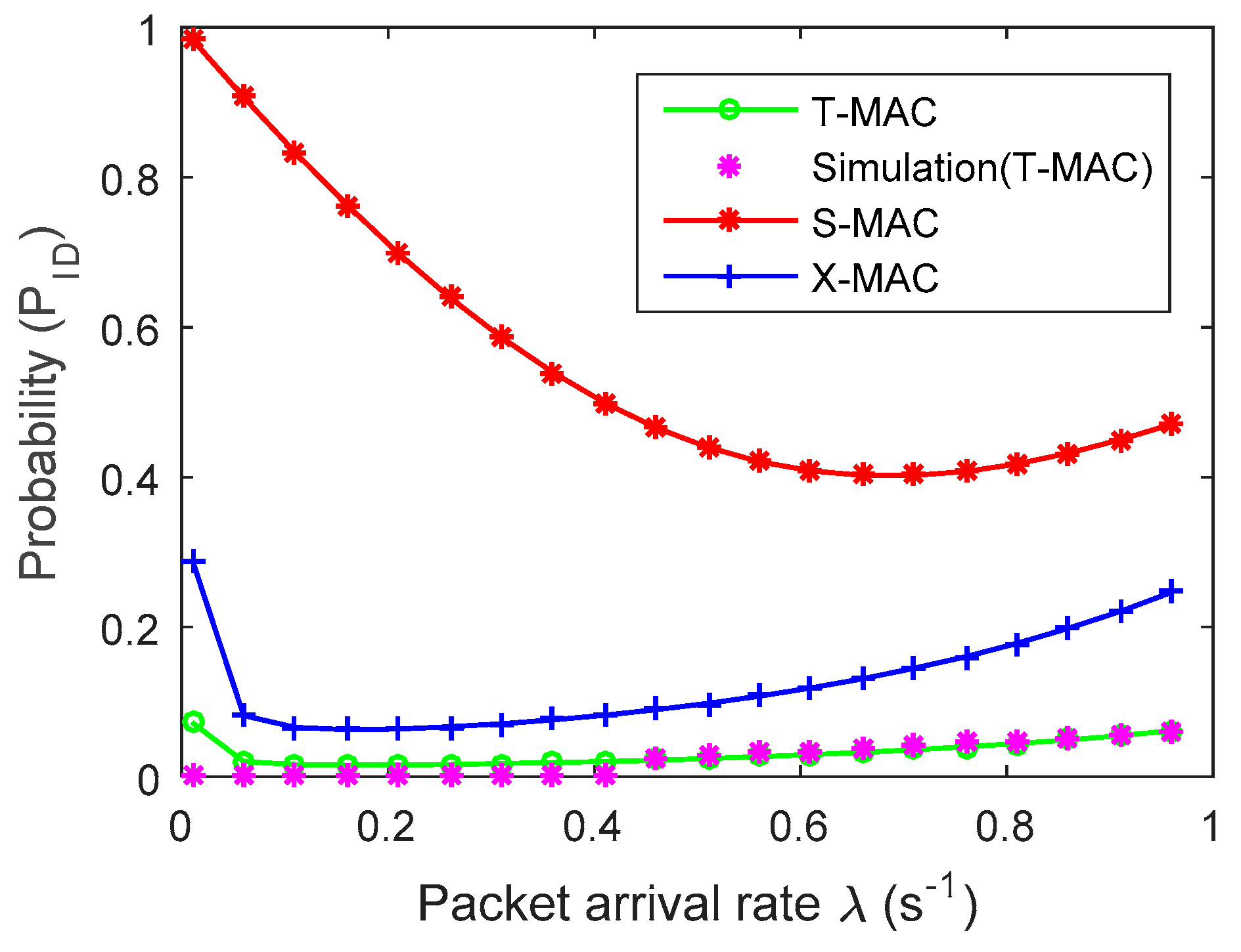
• A comparative performance analysis is done with the aid of a simulation to assess the energy efficiency of the suggested model, as compared to the state-of-the-art S-MAC and X-MAC based techniques, in view of various metrics.

The rest of this paper is organized as follows: Section 2 critically analyses the existing associated literatures on the MAC-based WSN energy optimization. The details of the proposed discrete-time Markov chain analytical model of the T-MAC protocol are presented in Section 3. The analytical and experimental results, with the comparative performance evaluation, are discussed in Section 4, which is later followed by the conclusions in Section 5.

2. Related Works

2.1. MAC Orientated Green Communication

In recent years, the focus has been on developing energy efficient MAC protocols for WSNs. The sleep and wake-up time cycle has been incorporated in the IEEE 802.11-distributed coordination function to conserve the energy of a sensor node. Various protocols are proposed in wireless sensor networks, like S-MAC, T-MAC, X-MAC and IEE 802.15, which are variants of IEEE 802.11, to conserve the energy at the MAC layer. In the past, there have been some analytical models that are proposed for the analysis of the performance of these MAC protocols on the basis of sleeping nodes. In [20], a mathematical model has been proposed for the S-MAC protocol to evaluate the throughput, delay and energy consumption under unsaturated traffic conditions. The authors considered the various factors together, including the active and sleep time cycle, the back off method, and the different traffic patterns for the S-MAC protocol. The modelling of the states of a node is done using a discrete time Markov chain, and the M/G/1/∞ queueing theory has been applied to compute the service delay, throughput, and energy consumption under unsaturated traffic conditions. A Markov queuing model has been proposed for the S-MAC and X-MAC protocols to calculate the throughput, delay, and energy consumption of both the synchronized duty-cycled S-MAC protocol and the asynchronous duty-cycled X-MAC protocol in [21]. The synchronous and asynchronous duty-cycled nodes queueing behaviour is studied using the Markov queueing model, as suggested by some authors. The performance evaluation of the synchronized duty-cycled S-MAC and asynchronous duty-cycled X-MAC protocols is calculated for the stationary probabilities of the packet transmission.

In [22], the authors evaluated the performance of the IEEE802.15.4 protocol, which takes retransmission and acknowledgements under unsaturated traffic conditions as parameters using a Markov chain model. In this analytical model, the network performance has been measured in terms of the frame delivery ratio, average power consumption of a node, channel throughput and frame discard ratio. The authors in [23] modelled the IEEE 802.15.4 MAC layer as a non-persistence carrier sense multiple access with a back off to compute the throughput and energy efficiency of the contention access period, and they proved that switching the radio into sleep mode between transmissions conserves the energy of the MAC layer. In [24], the performance of the IEEE 802.15.4 MAC protocol was dispensed within the terms of energy and throughput, in view of the right channel conditions under saturated and unsaturated traffic conditions. In [25], the authors estimated the delay and energy consumption of the IEEE 802.15.4 MAC layer, showing that the overall performance of the proposed model depends on the collision probability. In [26], an energy model is proposed to compute the power consumption, using the time-slotted channel hoping scheme that is the core of the IEEE 802.15.4e-2012 amendment of the IEEE 802.15.4-2011 standard.

2.2. Routing Orientated Green Communication

An approach for green computing has been proposed in [27] using Huffman coding-based ant colony optimization for a randomly distributed wireless sensor network. In particular, ant colony optimization is used to explore multiple paths, and Huffman coding is used to select the best path in view of the impact of two parameters on the energy consumption; namely, the path length and residual energy of each node. Green computing is performed in [28] by equalizing the energy consumption of all the sensors in the networks. A distributed forward search space was introduced to reduce the unnecessary transmission. Furthermore, four parameters, residual energy, node degree, distance and angle, have been used to construct the next forwarder selection function to select the next hop to route the packets. In [29], an energy balanced model was proposed to realize an equal distribution of energy consumption among all of the sensors in the network. New methods are proposed for the sensors to adjust the transmission range, adaptive sensing and density control to achieve a fair equalization of the energy consumption. Additionally, algorithms are presented for the annulus formation, connectivity ensured routing and coverage preserved scheduling, for the realization of a proposed energy balanced model. In [30], a new approach for green computing was presented, as a lifetime maximization based on balanced tree node switching. Two methods of shifting the nodes to achieve the balance tree of the node in the network, in terms of energy, were proposed. The author in [31] proposed a fault tolerance optimization method to minimize any end-to-end communication delay and fault tolerance in the wireless sensor network. An adaptive non-dominated sorting based genetic algorithm was used to solve the optimization problem. An analytical model of the T-MAC protocol was proposed in [32]. The authors in this paper estimated the length of the active and sleep time of a cycle time assuming that the occurrence of events follows the Poisson distribution. In this model, the energy consumption has been evaluated in terms of transmitting and receiving packets during the active time of a node. However, this model could not consider the back off mechanism. Furthermore, this analytical model could not calculate the service delay, throughput and power efficiency. Therefore, an analytical model that considers the back off mechanism, delay, throughput, and power efficiency under unsaturated traffic conditions needs to be developed.

3. Analytical Model of T-MAC Protocol

Here, we present a one-dimensional discrete time Markov queueing model of T-MAC for duty-cycled nodes with a variable cycle length. We consider the service delay, throughput, energy consumption and power efficiency for a node, according to the following assumptions: (a) a large number of arrivals of packets at each node are independent and discrete; therefore, the arrival of packets follows the Poisson distribution, (b) A large number of data packets is buffered by each node, (c) the packet retransmission is not endorsed here, (d) the channel is considered perfect (no fading), and (e) the deployment of sensor nodes follows the geometric distribution.

3.1. Node Behaviour Model

In this analytical model, a single hop WSN is considered, with n number of identical sensor nodes. The change of the node’s back off (BO) period is represented using the stochastic process. As per the T-MAC protocol, the back off timer is cancelled by the node if it fails to seize the channel in a cycle time, after which it will set a new BO timer for the next cycle. Hence, the stochastic process can be demonstrated with the discrete time Markov chain, as shown in Figure 1.

Consider that the proposed Markov chain has a finite number of states that are equal to the size W of the contention window. These states are numbered 0, 1, 2, 3 …, W−1, representing the status of the nodes. The parameters are considered in the model, as shown in

Table 1. Notations.

Notation	Description	Notation	Description
n	Number of sensor nodes	$E_{SL}$	Sleeping energy
W	Contention window size	$P_{SL}$	Probability of sleeping
p	Probability	$T_{COL}$	Collision time
${\mathsf{\Pi }}_{(.)}$	State probability	$T_{ID}$	Idle time
$k$	Positive integer	$T_{SL}$	Sleep time
$P_{TR}$	Probability of transmission	$T_{ST}$	Successful transmission time
$P_{ST}$	Probability of successful transmission	${\mathrm{T}}_1$	Missing transmission time
$P_{COL}$	Probability of collision	${\mathrm{T}}_2$	Time taken by the node for not capturing the channel
$P_{ID}$	Probability of idle	${\mathrm{T}}_3$	Time taken due to the back off procedure
$\mathsf{\tau }$	Time slot	${\mathrm{T}}_4$	Transmission time
$E_{ST}$	Energy consumption in successful transmission	${\mathrm{T}}_{\mathrm{CL}}$	Duration of a cycle
$E_{ID}$	Idle energy	${\mathrm{T}}_{\mathrm{A}}$	Threshold
$E_{COL}$	Collision energy	$\mathrm{E}$	Whole network energy
${\mathrm{T}}_{\mathrm{sam}}$	Sampling time in µs	S	Throughput
${\mathrm{T}}_{\mathrm{s}}$	Average transmission time	${\mathrm{R}}_{\mathrm{sam}}$	Sampling rate in µs

. The random back off timer is less than or equal to the current time slot. The transmission begins as soon as the back off period reaches zero. The back off period is chosen randomly in the range of [0, W−1] for each transmission. All of the sensor nodes sense the medium with an equal probability 1/W to capture the channel. If the channel is found to be idle, then a node contains the particular time slot which is equal to the current back off timer. The node continuously senses, with a probability (1−p), until the back off duration becomes zero, and it also ensures that no one is transmitting on the channel, after which it starts transmitting with probability 1. After the completion of the packet transmission, the node receives an acknowledgment (ACK) packet and then goes for back off duration with probability p. In the event that the channel seems busy, the node goes to back off duration with probability p. Again, the same process is repeated to capture the channel. The steady state equations of the discrete-time Markov chain are expressed as:

$${\mathsf{\Pi }}_0=\left(1/\mathrm{W}\right){\mathsf{\Pi }}_{BO}+\left(1-\mathrm{p}\right){\mathsf{\Pi }}_1$$

(1)

$${\mathsf{\Pi }}_1=\left(1/\mathrm{W}\right) {\mathsf{\Pi }}_{BO}+ \left(1-p\right){\mathsf{\Pi }}_2.$$

(2)

Similarly, for the $kth$ state, the balance equation is given by Equation (3):

$${\mathsf{\Pi }}_k=\left(1/\mathrm{W}\right){\mathsf{\Pi }}_{BO}+ \left(1-p\right){\mathsf{\Pi }}_{k+1}$$

(3)

$${\mathsf{\Pi }}_{BO}={\mathrm{p}\mathsf{\Pi }}_{ACK}+ p{\mathsf{\Pi }}_0+{\mathrm{p}\mathsf{\Pi }}_1+\dots +{\mathrm{p}\mathsf{\Pi }}_{W-1}$$

(4)

$${\mathsf{\Pi }}_{ACK}={\mathsf{\Pi }}_0$$

(5)

$${\mathsf{\Pi }}_{ACK}+{\mathsf{\Pi }}_{BO}+{\displaystyle \sum }_{k=0}^{W-1}{\mathsf{\Pi }}_k=1,$$

(6)

where $k$ takes the positive integer value from 0 to W−1, and ${\mathsf{\Pi }}_{(.)}$ represents the state probability. Upon solving the above equations, we have:

$$\begin{gathered} \begin{array}{ll}{\mathsf{\Pi }}_0= \left(1/\mathrm{W}\right){\mathsf{\Pi }}_{BO}& +\left(1-\mathrm{p}\right)\left[\left(1/\mathrm{W}\right){\mathsf{\Pi }}_{BO}+\left(1-\mathrm{p}\right){\mathsf{\Pi }}_2\right]\\ & = \left(2-\mathrm{p}\right)\left(1/\mathrm{W}\right){\mathsf{\Pi }}_{BO}+{\left(1-\mathrm{p}\right)}^2{\mathsf{\Pi }}_2\\ & = \left(2-\mathrm{p}\right)\left(1/\mathrm{W}\right){\mathsf{\Pi }}_{BO}++{\left(1-\mathrm{p}\right)}^2\left(1/\mathrm{W}\right){\mathsf{\Pi }}_{BO}+\dots {\left(1-\mathrm{p}\right)}^{\mathrm{k}}{\mathsf{\Pi }}_k\\ & = \left(\frac{1}{\mathrm{W}}\right){\mathsf{\Pi }}_{BO}[\left(2-\mathrm{p}\right)+{\left(1-\mathrm{p}\right)}^2+\dots +{\left(1-\mathrm{p}\right)}^{\mathrm{k}-1}]+{\left(1-\mathrm{p}\right)}^{\mathrm{k}}{\mathsf{\Pi }}_k\\ & = \left(\frac{1}{\mathrm{W}}\right){\mathsf{\Pi }}_{BO}[1+\left(1-\mathrm{p}\right)+{\left(1-\mathrm{p}\right)}^2+\dots {\left(1-\mathrm{p}\right)}^{\mathrm{k}-1}]+{\left(1-\mathrm{p}\right)}^{\mathrm{k}}{\mathsf{\Pi }}_k\\ & = \left(\frac{1}{\mathrm{W}}\right){\mathsf{\Pi }}_{BO}+[\frac{1-{\left(1-\mathrm{p}\right)}^{\mathrm{k}-1}}{\mathrm{p}}]+ {\left(1-\mathrm{p}\right)}^{\mathrm{k}}{\mathsf{\Pi }}_k=\end{array} \\ {\mathsf{\Pi }}_k=[{\mathsf{\Pi }}_0-(\frac{1}{\mathrm{W}}){\mathsf{\Pi }}_{BO}\{\frac{1-{\left(1-\mathrm{p}\right)}^{\mathrm{k}-1}}{\mathrm{p}}\}]\frac{1}{{\left(1-\mathrm{p}\right)}^{\mathrm{k}}} \\ {\mathsf{\Pi }}_k{\left(1-\mathrm{p}\right)}^{\mathrm{k}}= {\mathsf{\Pi }}_0-(\frac{1}{\mathrm{W}}){\mathsf{\Pi }}_{BO}\{\frac{1-{\left(1-\mathrm{p}\right)}^{\mathrm{k}-1}}{\mathrm{p}}\}. \end{gathered}$$

(7)

To normalize, we solve Equations (6) and (7), which is to say we put the value of ${\mathsf{\Pi }}_{BO}$ from Equation (6) into Equation (7), and we get:

$$\begin{array}{l}{\mathsf{\Pi }}_k{\left(1-\mathrm{p}\right)}^{\mathrm{k}}= {\mathsf{\Pi }}_0-\left(\frac{1}{\mathrm{W}}\right)\{1-{\displaystyle \sum }_{\mathrm{k}=0}^{\mathrm{W}-1}{\mathsf{\Pi }}_k\}\{\frac{1-{\left(1-\mathrm{p}\right)}^{\mathrm{k}-1}}{\mathrm{p}}\}\\ {\mathsf{\Pi }}_k{\left(1-\mathrm{p}\right)}^{\mathrm{k}}={\mathsf{\Pi }}_0\{1+\left(\frac{1}{\mathrm{W}}\right)\{\frac{1-{\left(1-\mathrm{p}\right)}^{\mathrm{k}-1}}{\mathrm{p}}\}-\left(\frac{1}{\mathrm{W}}\right)\{1{\displaystyle {\displaystyle \sum }_{\mathrm{k}=0}^{\mathrm{W}-1}}{\mathsf{\Pi }}_k\}\{\frac{1-{\left(1-\mathrm{p}\right)}^{\mathrm{k}-1}}{\mathrm{p}}\}\end{array}$$

$$\begin{array}{ll}{\mathsf{\Pi }}_0& =\frac{\Pi \left(state k\right)+\left(\frac{1}{W}\right)\left\{1-{{\displaystyle \sum }}_{k=0}^{W-1}{\mathsf{\Pi }}_k\right\}\left\{\frac{1-{\left(1-p\right)}^{k-1}}{p}\right\}}{1+\left\{\frac{1-{\left(1-p\right)}^{k-1}}{Wp}\right\}}\\ & = \frac{\frac{1}{\mathrm{W}}+\left(\frac{1}{\mathrm{W}}\right)\left\{1-{{\displaystyle \sum }}_{\mathrm{k}=0}^{\mathrm{W}-1}\left(\frac{1}{\mathrm{W}}\right)\right\}\left\{\frac{1-{\left(1-\mathrm{p}\right)}^{\mathrm{W}-1-1}}{\mathrm{p}}\right\}}{1+\left\{\frac{1-{\left(1-\mathrm{p}\right)}^{\mathrm{W}-1-1}}{\mathrm{Wp}}\right\}}\\ & = \frac{\frac{1}{\mathrm{W}}+\left(\frac{1}{\mathrm{W}}\right)\left\{1-\left(\frac{1}{\mathrm{W}}\right){{\displaystyle \sum }}_{\mathrm{k}=0}^{\mathrm{W}-1}\left(1\right)\right\}\left\{\frac{1-{\left(1-\mathrm{p}\right)}^{\mathrm{W}-2}}{\mathrm{p}}\right\}}{1+\left\{\frac{1-{\left(1-\mathrm{p}\right)}^{\mathrm{W}-2}}{\mathrm{Wp}}\right\}}\\ & =\frac{\frac{1}{\mathrm{W}}+\left(\frac{1}{\mathrm{W}}\right)\left\{1-\left(\frac{1}{\mathrm{W}}\right)\left(\mathrm{W}-1\right)\right\}\left\{\frac{1-{\left(1-\mathrm{p}\right)}^{\mathrm{W}-2}}{\mathrm{p}}\right\}}{1+\left\{\frac{1-{\left(1-\mathrm{p}\right)}^{\mathrm{W}-2}}{\mathrm{Wp}}\right\}}\\ & = \frac{\mathrm{p}+\left(\frac{1}{\mathrm{W}}\right)\left\{\frac{1-{\left(1-\mathrm{p}\right)}^{\mathrm{W}-2}}{\mathrm{p}}\right\}}{1+\left\{\frac{1-{\left(1-\mathrm{p}\right)}^{\mathrm{W}-2}}{\mathrm{Wp}}\right\}}.\end{array}$$

The transmission probability is given by:

$${\mathsf{\Pi }}_0=\frac{\mathrm{p}+\left(\frac{1}{\mathrm{W}}\right)\left\{1-{\left(1-\mathrm{p}\right)}^{\mathrm{W}-2}\right\}}{1+\mathrm{p}-{\left(1-\mathrm{p}\right)}^{\mathrm{W}-2}},$$

(8)

where $p$ represents the probability that among the remaining n−1 sensor nodes, at least one will transmit in a time slot given by $p=1-{\left(1-{\mathsf{\Pi }}_0\right)}^{n-1}$.

3.2. Cycle Probability Model

A cycle can be characterized by the event that happens within the cycle. The events are an idle cycle, a successful transmission cycle, and an unsuccessful transmission cycle/collision cycle. When the sensors have no packet to transmit, it is termed an idle cycle. On the other hand, when one of the sensors, having a packet which requires transmission, attains the channel and transmits the packet successfully, it is called a successful transmission cycle; furthermore, when more than one sensor selects the same back off period and causes an RTS collision, it is termed a collision cycle. We assume that $P_{TR}$ is the probability of at least one transmission of n active sensor nodes in a time slot, $P_{ST}$ is the probability that a transmission is successful, $P_{COL}$ is the collision probability, $P_{ID}$ is the idle probability and $P_{SL}$ is the sleeping probability; these are given as:

$$P_{TR}=1-{\left(1-{\Pi }_0\right)}^n$$

(9)

$$P_{ST}=\frac{n {\Pi }_0{\left(1-{\Pi }_0\right)}^{n-1}}{P_{TR}}$$

(10)

$$P_{COL}={\left(1-{\Pi }_0\right)}^n{\displaystyle \sum }_{k=0}^n\left(\begin{array}{c}n\\ k\end{array}\right){(P_{TR})}^k{\left(1-P_{TR}\right)}^{n-k}$$

(11)

$$P_{ID}=\frac{{\Pi }_0}{P_{ST}}$$

(12)

$$P_{SL}=\left(1-P_{TR}\right)\left(1-P_{ID}\right)$$

(13)

3.3. Throughput Analysis

The throughput S is defined as the total time to the time when the channel was used for transmitting the payload bits successfully. The time for the collision, sleeping time, time for the successful transmission and idle time are four fractions of the time when a slot of some random time is chosen. Thus, the throughput expression $S$ is given by:

$$S=\frac{P_{tr}{P}_{ST}E\left[P\right]}{\left(1-P_{TR}{P}_{ST}-P_{COL}\right)+P_{TR}{P}_{ST}{T}_{ST}+P_{COL}{T}_{COL}+P_{SL}{T}_{SL}+P_{ID}{T}_{ID}},$$

(14)

where E[P] is represented by the average packet payload size. The times $T_{COL},$ $T_{ID}$, $T_{SL}$ and $T_{ST}$ are the times for the collision, idle, sleep and successful transmissions for the busy channel, respectively.

3.4. Service Delay Analysis

The service delay is a significant measurement in low-rate traffic. The time from the arrival of the packet to the reception of the packet is termed the service delay or packet service time. We show all time consumption in terms of the back off period, which has the following components: (1) ${\mathrm{T}}_1,$ represented as the time taken due to missing the transmission opportunity as a result of sleeping; (2) ${\mathrm{T}}_2,$ represented as the time taken by the node for not capturing the channel and for not being able to successfully transmit during the cycle; (3) ${\mathrm{T}}_3,$ represented as the time taken due to the back off procedure for the successful transmission in a cycle; and (4) ${\mathrm{T}}_4$ is the time required for a represented transmission. It is assumed that the duration of a cycle is denoted by ${\mathrm{T}}_{\mathrm{CL}}$, the time slot by $\mathsf{\tau }$; furthermore, the minimum idle time (threshold) to change the states of the sensor from active to sleep is denoted by ${\mathrm{T}}_{\mathrm{A}}$. Following this, the sleep time of a node can be represented as:

$$T_{SL}={\mathrm{T}}_{\mathrm{CL}}-\left({\mathrm{T}}_{\mathrm{TR}}+{\mathrm{T}}_{\mathrm{A}}\right).$$

(15)

Let us define G(z) as a probability generating function (PGF) of the packet service time:

$$G\left(z\right)= {\displaystyle \sum }_{i=0}^{W-1}{P}_{TR} Z^i+{\displaystyle \sum }_{i=0}^{T_{ST}}{P}_{ST} Z^i+{\displaystyle \sum }_{i=0}^{T_{ID}}{P}_{ID} Z^i+{\displaystyle \sum }_{i=0}^{T_{SL}}{P}_{SL} Z^i$$

(16)

$$\frac{dG\left(z\right)}{dz}= {\displaystyle \sum }_{i=0}^{W-1}{P}_{TR} i Z^{i-1}+{\displaystyle \sum }_{i=0}^{T_{ST}}{P}_{ST}i Z^{i-1}+{\displaystyle \sum }_{i=0}^{T_{ID}}{P}_{ID}i Z^{i-1}+{\displaystyle \sum }_{i=0}^{T_{SL}}{P}_{SL} i Z^{i-1}$$

(17)

Therefore, the average service delay is given as:

$$\mathrm{E}\left(G\right)={\frac{dG\left(z\right)}{dz}|}_{Z=1}=\frac{1}{2}[P_{TR} W\left(W-1\right)+P_{ST} T_{ST}\left(T_{ST}+1\right)+ P_{ID} T_{ID}\left(T_{ID}+1\right)+P_{SL}{T}_{SL} \left(T_{SL}+1\right)]$$

(18)

3.5. Energy Consumption and Power Efficiency

The whole network energy consumption during a cycle is given as:

$$\mathrm{E}=E_{ST}{P}_{ST}+E_{ID}{P}_{ID}+E_{COL}{\mathrm{P}}_{\mathrm{COL}}+E_{SL}{P}_{SL}$$

(19)

On substituting the values of ${\mathrm{P}}_{ST}$, ${\mathrm{P}}_{\mathrm{ID}}$, ${\mathrm{P}}_{COL}$ and ${\mathrm{P}}_{SL}$ from Equations (10), (11), (12) and (13) in (19), the energy consumption E for the whole network can be determined. $E_{ST}$, $E_{ID}$, $E_{COL}$ and $E_{SL}$ are the energy consumption in a successful transmission cycle, in the idle state, in collision, and in the sleep state, respectively. The throughput attained per unit of energy consumed is termed as power efficiency and is represented as:

$$Power efficiency = \frac{ Throughput}{Total energy consumption}=\frac{S}{E}$$

(20)

4. Experimental Results and Analysis

The analytical results obtained for the proposed analytical model of T-MAC are presented and compared with those of the analytical model of the S-MAC and X-MAC protocols. Furthermore, the analytical results of T-MAC have been validated by conducting the simulation for the T-MAC protocol. The nodes are randomly deployed in the network field, which has an area of 200 × 200 m². The number of sensors deployed for this simulation is 50. The radio range of the sensor is assumed to be 50 m. The data packet size is taken to be 512 bits. The packet arrival rate follows the Poison process. The results provide an analysis for the probabilities of a successful transmission cycle, energy consumption, idle cycle, average service delay, throughput, collision cycle, and power efficiency for the different packet arrival rates ⋋. It is assumed that there are $n$ = 4 sensors, contending for the channel access, with a contention window size of $\mathrm{W}=16$. The energy consumed per unit of time for a successful transmission, idle state, collision, and sleep state is assumed to be $E_{ST}$ = 5 mJ, $E_{ID}$ = 0.2 mJ, $E_{COL}$ = 7 mJ and $E_{SL}$ = 0.04 mJ, respectively. The time is divided into a number of slots of length $\mathsf{\tau }$ = 10 s. The cycle length is assumed to be ${\mathrm{T}}_{\mathrm{cl}}$ = 30 µs. The sensor goes into sleep mode if no event occurred for a certain time of idle listening that assumed to be ${\mathrm{T}}_{\mathrm{A}}$ = 1 µs. The average transmission time of the sensors is assumed to be ${\mathrm{T}}_{\mathrm{s}}$ = 5 µs. The signal sampling time and rate are assumed to be ${\mathrm{T}}_{\mathrm{sam}}$ = 5 µs and ${\mathrm{R}}_{\mathrm{sam}}$ = 2 µs.

Figure 2 shows the comparison of the idle probability in a cycle with respect to the different packet arrival rates for the T-MAC, S-MAC and X-MAC protocols. It is observed that for T-MAC, with the increase of the packet arrival rate, the idle probability of a sensor increases very slowly; however, for S-MAC, it decreases sharply. This is due to the fact that the idle listening time for the T-MAC protocol is fixed, which is to say it avoids idle listening during the active time, and the sensor goes to sleep mode if there is no event happening for a certain time of idle listening. In other words, due to the lower idle listening time, the T-MAC protocol has a lower energy consumption when compared to the S-MAC protocol. It is seen that the ideal probability of the sensor is lower than that of S-MAC and X-MAC. For example, for the packet arrival rate ⋋ = 0.4, the idle probability $P_{ID}$ is 0.05 for T-MAC, whereas for X-MAC and S-MAC it is 0.09 and 0.5, respectively.

Figure 3 shows the comparison of the collision probability $P_{COL}$, with respect to the packet arrival rate ⋋ for the T-MAC, S-MAC and X-MAC protocols. It is perceived that, with the increase in the arrival rate, the collision probability packet also increases for all of the protocols considered for comparison. The collision probability of the T-MAC protocol is much less when compared to the S-MAC and X-MAC protocols. For example, for the packet arrival rate ⋋ = 0.8, the collision probability for T-MAC is 0.00025, whereas for S-MAC and X-MAC, it is 0.001 and 0.00075, respectively. This is due to the fact that for a high packet arrival rate, the active time for T-MAC becomes longer than that of S-MAC and X-MAC. T-MAC sends more data in a successful cycle time, whereas a higher number of successful cycles for S-MAC is required to send the same amount of data. In other words, the number of trials to reserve the medium for S-MAC and X-MAC is higher than for T-MAC.

Figure 4 shows the comparison of the successful transmission probability $P_{ST},$ with respect to the packet arrival rate ⋋ for the T-MAC, S-MAC and X-MAC protocols. The probability of a successful transmission for both of the protocols is directly proportional to the packet arrival rate. The rate of increments in the successful transmissions for T-MAC is higher than that of S-MAC and X-MAC. For example, for the packet arrival rate ⋋ = 0.2, the successful transmission probability for T-MAC is 0.5, whereas for S-MAC and X-MAC it is 0.1 and 0.25, respectively. Similarly, for the packet arrival rate ⋋ = 0.6, the successful transmission probability for T-MAC is 0.7, whereas for S-MAC and X-MAC it is 0.23 and 0.48, respectively. This is due to the fact that T-MAC transmits a higher number of packets in the active time than S-MAC does.

Figure 5 shows the comparison of the T-MAC, S-MAC and X-MAX protocols for the average service delay with respect to different packet arrival rates ⋋ for the T-MAC, S-MAC and X-MAC protocols. It is witnessed in the protocols that the average service delay of T-MAC increases slower when compared with that of the S-MAC and X-MAX protocols for an increasing packet arrival rate ⋋. For example, for the packet arrival rate ⋋ = 0.2, the average service delay for T-MAC is 20 s, whereas for S-MAC and X-MAC it is 30 and 125 s, respectively. Similarly, for the packet arrival rate ⋋ = 0.6, the average service delay for T-MAC is 75 s, whereas for S-MAC and X-MAC it is 110 and 150 s, respectively. This is due to the following reason: the increment in the packet arrival rate increases the active time of a cycle for T-MAC, which ultimately increases the transmission of the packets. Therefore, the average service delay is lower than for S-MAC and X-MAC.

Figure 6 shows the throughput with respect to the different packet arrival rates for the T-MAC, S-MAC and X-MAC protocols. It is witnessed that before the node becomes saturated for the T-MAC, S-MAC and X-MAC protocols, the overall throughput increments linearly with the packet arrival rate up to 0.2. Thereafter, the throughputs for all of the protocols start decreasing with an increasing packet arrival rate. The throughput of the T-MAC protocol is better than that of the S-MAC and X-MAC protocols. For example, for the packet arrival rate ⋋ = 0.2, the throughput for T-MAC is 0.25, whereas for S-MAC and X-MAC it is 0.04 and 0.12, respectively. Similarly, for the packet arrival rate ⋋ = 0.6, the throughput for T-MAC is 0.2, whereas for S-MAC and X-MAC it is 0.09 and 0.12, respectively. This is due to the fact that a higher packet arrival rate increases the active time of a cycle for the T-MAC.

Figure 7 demonstrates the correlation of the average energy consumption with respect to the packet arrival rate ⋋ for the T-MAC, S-MAC and X-MAC protocols. From Figure 7, it is seen that a higher traffic load has induced a larger energy consumption for all of the protocols. However, the T-MAC protocol consumes less energy that S-MAC and X-MAC do. For example, for the packet arrival rate ⋋ = 0.4, the average energy consumption for T-MAC is 100 mJ, whereas for S-MAC and X-MAC it is 280 mJ and 190 mJ, respectively. Similarly, for the packet arrival rate ⋋ = 0.6, the average energy consumption for T-MAC is 170 mJ, whereas for S-MAC and X-MAC it is 425 mJ and 300 mJ, respectively. This is because the sensors in S-MAC sense the channel throughout the active duration in each idle cycle, which consumes a lot of the protocol’s energy. In T-MAC, the idle listening varies with the packet arrival rate. If the packet arrival rate is high, the sensor nodes remain alert in order to deal with the packets.

Figure 8 shows the comparison of the power efficiency with respect to the packet arrival rate ⋋ for the T-MAC, S-MAC and X-MAC protocols. It is observed in Figure 8 that the power efficiency for the T-MAC protocol is better than for the S-MAC and X-MAC protocols. The overall power efficiency increases linearly with the packet arrival rate, up to 0.24. Thereafter, the power efficiencies for all of the protocols start decreasing with an increasing packet arrival rate. The power efficiency of the T-MAC protocol is better than that of the S-MAC and X-MAC protocols. For example, for the packet arrival rate ⋋ = 0.2, the power efficiency for T-MAC is 0.3, whereas for S-MAC and X-MAC it is 0.06 and 0.2, respectively. Similarly, for the packet arrival rate ⋋ = 0.6, the power efficiency for T-MAC is 0.17, and it also equal to that of X-MAC. On the other hand, the power efficiency for S-MAC is 0.08. The power efficiency for all of the three protocols converges to 0.05 for a packet arrival rate of 1. This is because a higher number of packets arriving in the network increases the collisions and consumes more of the nodes’ energy in order to reserve the channel. Hence, T-MAC saves more power in comparison to the S-MAC and X-MAC protocols.

5. Conclusions

An analytical model is proposed in this paper to analyse the performance of the T-MAC protocol under unsaturated traffic conditions. The proposed analytical model is also validated by conducting a simulation. Furthermore, a one-dimensional discrete time Markov queueing model has been presented in this paper in order to represent the back-off process of duty-cycled sensor nodes. The probabilities of a successful transmission, collision, and idle state of a sensor node are computed. The M/M/1/∞ model is proposed to analyse the throughput of the T-MAC protocol under unsaturated traffic conditions. The energy consumption model has been presented, using the probabilities of a successful transmission, collision, and idle state of a sensor node. The proposed analytical model is matched with the existing analytical model of the S-MAC and X-MAC protocols. Our analysis shows that the proposed model of T-MAC achieves a healthier throughput and saves more energy than the existing model of the S-MAC and X-MAC protocols.

References

1. Kaiwartya, O.; Abdullah, A.H.; Cao, Y.; Raw, R.S.; Kumar, S.; Lobiyal, D.K.; Isnin, I.F.; Liu, X.; Shah, R.R. T-MQM: Testbed-based multi-metric quality measurement of sensor deployment for precision agriculture—A case study. IEEE Sens. J. 2016, 16, 8649–8664. [Google Scholar] [CrossRef]
2. Ullah, F.; Abdullah, A.H.; Kaiwartya, O.; Cao, Y. TraPy-MAC: Traffic priority aware medium access control protocol for wireless body area network. J. Med Syst. 2017, 41, 93. [Google Scholar] [CrossRef] [PubMed]
3. Ahmed, M.N.; Abdullah, A.H.; Kaiwartya, O. FSM-F: Finite state machine based framework for denial of service and intrusion detection in MANET. PLoS ONE 2016, 11, e0156885. [Google Scholar] [CrossRef]
4. Qureshi, K.N.; Abdullah, A.H.; Kaiwartya, O.; Iqbal, S.; Butt, R.A.; Bashir, F. A Dynamic congestion control scheme for safety applications in vehicular ad hoc networks. Comput. Electr. Eng. 2018, 72, 774–788. [Google Scholar] [CrossRef]
5. Hassan, A.N.; Kaiwartya, O.; Abdullah, A.H.; Sheet, D.K.; Raw, R.S. Inter vehicle distance based connectivity aware routing in vehicular adhoc networks. Wirel. Pers. Commun. 2018, 98, 33–54. [Google Scholar] [CrossRef]
6. Cao, Y.; Kaiwartya, O.; Zhuang, Y.; Ahmad, N.; Sun, Y.; Lloret, J. A decentralized deadline-driven electric vehicle charging recommendation. IEEE Syst. J. 2018, 99, 1–12. [Google Scholar] [CrossRef]
7. Cao, Y.; Wang, T.; Zhang, X.; Kaiwartya, O.; Eiza, M.H.; Putrus, G. Toward anycasting-driven reservation system for electric vehicle battery switch service. IEEE Syst. J. 2019, 13, 906–917. [Google Scholar] [CrossRef]
8. Farhan, L.; Kharel, R.; Kaiwartya, O.; Hammoudeh, M.; Adebisi, B. Towards green computing for internet of things: Energy oriented path and message scheduling approach. Sustain. Cities Soc. 2018, 38, 195–204. [Google Scholar] [CrossRef]
9. Kaiwartya, O.; Abdullah, A.H.; Cao, Y.; Altameem, A.; Prasad, M.; Lin, C.T.; Liu, X. Internet of vehicles: Motivation, layered architecture, network model, challenges, and future aspects. IEEE Access 2016, 4, 5356–5373. [Google Scholar] [CrossRef]
10. Kaiwartya, O.; Kumar, S.; Abdullah, A.H. Analytical model of deployment methods for application of sensors in non-hostile environment. Wirel. Pers. Commun. 2017, 97, 1517–1536. [Google Scholar] [CrossRef]
11. Khasawneh, A.; Latiff, M.; Kaiwartya, O.; Chizari, H. Next forwarding node selection in underwater wireless sensor networks (UWSNs): Techniques and challenges. Information 2016, 8, 3. [Google Scholar] [CrossRef]
12. Khatri, A.; Kumar, S.; Kaiwartya, O. Optimizing energy consumption and inequality in wireless sensor networks using NSGA-II. In Proceedings of the ICCCS, Boca Raton, FL, USA, 10 September 2016. [Google Scholar]
13. Kumar, V.; Kumar, S. Position-based beaconless routing in wireless sensor networks. Wirel. Pers. Commun. 2016, 86, 1061–1085. [Google Scholar] [CrossRef]
14. Kumar, K.; Kumar, S.; Kaiwartya, O.; Cao, Y.; Lloret, J.; Aslam, N. Cross-layer energy optimization for IoT environments: Technical advances and opportunities. Energies 2017, 10, 2073. [Google Scholar] [CrossRef]
15. .Holland, M.; Wang, T.; Tavli, B.; Seyedi, A.; Heinzelman, W. Optimizing physical-layer parameters for wireless sensor networks. ACM Trans. Sens. Netw. 2011, 7, 28. [Google Scholar] [CrossRef]
16. Khasawneh, A.; Latiff, M.S.B.A.; Kaiwartya, O.; Chizari, H. A reliable energy-efficient pressure-based routing protocol for underwater wireless sensor network. Wirel. Netw. 2018, 24, 2061–2075. [Google Scholar] [CrossRef]
17. Ullah, F.; Abdullah, A.H.; Kaiwartya, O.; Lloret, J.; Arshad, M.M. EETP-MAC: Energy efficient traffic prioritization for medium access control in wireless body area networks. Telecommun. Syst. 2017, 1–23. [Google Scholar] [CrossRef]
18. Ye, W.; Heidemann, J.; Estrin, D. Medium access control with coordinated adaptive sleeping for wireless sensor networks. IEEE Trans. Netw. 2004, 12, 493–506. [Google Scholar] [CrossRef]
19. Heinzelman, W.; Chandrakasan, A.; Balakrishnan, H. Energy-efficient communication protocols for wireless microsensor networks. In Proceedings of the 33rd Annual Hawaii International Conference on System Sciences, Maui, HI, USA, 7 January 2000; Volume 1, pp. 3005–3014. [Google Scholar]
20. Ye, Z.; He, C.; Ji, L. Performance analysis of S-MAC protocol under unsaturated conditions. IEEE Commun. Lett. 2008, 12, 210–212. [Google Scholar]
21. Yang, O.; Heinzelman, W.B. Modeling and performance analysis for duty-cycled MAC protocols with applications to S-MAC and X-MAC. IEEE Trans. Mob. Comput. 2012, 11, 905–921. [Google Scholar] [CrossRef]
22. Wijetunge, S.; Gunawardana, U.; Liyanapathirana, R. Performance analysis of IEEE 802.15.4 MAC protocol with ACK frame transmission. Wirel. Pers. Commun. 2013, 69, 509–534. [Google Scholar] [CrossRef]
23. Ramachandran, I.; Das, A.K.; Roy, S. Analysis of the contention access period of IEEE 802.15.4 MAC. ACM Trans. Sens. Netw. 2007, 3, 4. [Google Scholar] [CrossRef] [Green Version]
24. Pollin, S.; Ergen, M.; Ergen, S.C.; Bougard, B.; van der Perre, L.; Moerman, I.; Bahai, A.; Varaiya, P.; Catthoor, F. Performance analysis of slotted carrier sense IEEE 802.15.4 medium access layer. IEEE Trans. Wirel. Commun. 2008, 7, 3359–3371. [Google Scholar] [CrossRef]
25. Park, P.; Marco, P.D.; Soldati, P.; Fischione, C.; Johansson, K.H. A generalized Markov chain model for effective analysis of slotted IEEE 802.15.4. In Proceedings of the 2009 IEEE 6th International Conference on Mobile Adhoc and Sensor Systems, Macau, China, 12–15 October 2009; pp. 130–139. [Google Scholar]
26. Vilajosana, X.; Wang, Q.; Chraim, F.; Watteyne, T.; Chang, T.; Pister, K.S.J. A realistic energy consumption model for TSCH networks. IEEE Sens. J. 2014, 14, 482–489. [Google Scholar] [CrossRef]
27. Aanchal; Kumar, S.; Kaiwartya, O.; Abdullah, A.H. Green computing for wireless sensor networks: Optimization and Huffman coding approach. Peer Peer Netw. Appl. 2017, 10, 592–609. [Google Scholar] [CrossRef]
28. Kumar, V.; Kumar, S. Energy balanced position-based routing for lifetime maximization of wireless sensor networks. Ad Hoc Netw. 2016, 52, 117–129. [Google Scholar] [CrossRef]
29. Dohare, U.; Lobiyal, D.K.; Kumar, S. Energy balanced model for lifetime maximization for a randomly distributed sensor networks. Wirel. Pers. Commun. 2014, 78, 407–428. [Google Scholar] [CrossRef]
30. Khatri, A.; Kumar, S.; Kaiwartya, O. Towards green computing in wireless sensor networks: Controlled mobility-aided balanced tree approach. Int. J. Commun. Syst. 2018, 31, e3463. [Google Scholar] [CrossRef]
31. Kaiwartya, O.; Abdullah, A.H.; Cao, Y.; Lloret, J.; Kumar, S.; Shah, R.R.; Prasad, M.; Prakash, S. Virtualization in wireless sensor networks: Fault tolerant embedding for internet of things. IEEE Internet Things J. 2018, 5, 571–580. [Google Scholar] [CrossRef]
32. Ramchand, V.; Lobiyal, D.K. An analytical model for power control T-MAC protocol. Int. J. Comput. Appl. 2010, 12, 13–18. [Google Scholar] [CrossRef]
Figure 1. Discrete time Markov Chain of T-MAC Protocol.
Electronics 08 00534 g001
Figure 2. The idle probability P I D in a cycle versus the packet arrival rate ⋋ for the T-MAC, S-MAC and X-MAC protocols.
Electronics 08 00534 g002
Figure 3. The collision probability P C O L in a cycle versus the packet arrival rate ⋋ for the T-MAC, S-MAC and X-MAC protocols.
Electronics 08 00534 g003
Figure 4. The successful transmission probability, P S T , in a cycle versus different packet arrival rates ⋋, for the T-MAC, S-MAC and X-MAC protocols.
Electronics 08 00534 g004
Figure 5. The average service delay with respect to the packet arrival rate ⋋ for the T-MAC, S-MAC and X-MAC protocols.
Electronics 08 00534 g005
Figure 6. The throughput versus packet arrival rate ⋋ for the T-MAC, S-MAC and X-MAC protocols.
Electronics 08 00534 g006
Figure 7. The average energy consumption versus packet arrival rate for the T-MAC, S-MAC and X-MAC protocols.
Electronics 08 00534 g007
Figure 8. The power efficiency for T-MAC, S-MAC and X-MAC protocols versus packet arrival rate.
Electronics 08 00534 g008