Article

Green Computing in Sensors-Enabled Internet of Things: Neuro Fuzzy Logic-Based Load Balancing

1
School of Computer and Systems Sciences, Jawaharlal Nehru University, New Delhi 110067, India
2
Department of Computer Engineering, Delhi Technological University (DTU), New Delhi 110042, India
3
School of Engineering, Manchester Metropolitan University, Manchester M1 5GD, UK
*
Author to whom correspondence should be addressed.
Electronics 2019, 8(4), 384; https://doi.org/10.3390/electronics8040384
Submission received: 1 March 2019 / Revised: 23 March 2019 / Accepted: 25 March 2019 / Published: 29 March 2019
(This article belongs to the Special Issue Vehicular Networks and Communications)

Abstract

:
Energy is a precious resource in the sensors-enabled Internet of Things (IoT). Unequal load on sensors deplete their energy quickly, which may interrupt the operations in the network. Further, a single artificial intelligence technique is not enough to solve the problem of load balancing and minimize energy consumption, because of the integration of ubiquitous smart-sensors-enabled IoT. In this paper, we present an adaptive neuro fuzzy clustering algorithm (ANFCA) to balance the load evenly among sensors. We synthesized fuzzy logic and a neural network to counterbalance the selection of the optimal number of cluster heads and even distribution of load among the sensors. We developed fuzzy rules, sets, and membership functions of an adaptive neuro fuzzy inference system to decide whether a sensor can play the role of a cluster head based on the parameters of residual energy, node distance to the base station, and node density. The proposed ANFCA outperformed the state-of-the-art algorithms in terms of node death rate percentage, number of remaining functioning nodes, average energy consumption, and standard deviation of residual energy.

1. Introduction

Sensors enabled Internet of Things (IoT) networks have been regarded as reasonable data collection and control applications over various network communication infrastructures through smart sensors called IoT nodes [1,2,3]. Sensors-enabled IoT networks are comprised of various smart sensor nodes (RFID enabled) that assemble facts (data) from the encompassing conditions and convey the data to the static base station (BS) or overload the data to cloud applications where users download the data for processing [4,5,6]. Sensors-enabled IoT networks have gained impressive attention in view of their broad application in animal or human tracking and surveillance, medical environments [7], military services, automobile industries [8], stock administration in industrial production [9], environment monitoring, natural hazards and seismic detection, fleet navigation and management, agricultural advancements [10], etc. However, these smart sensor nodes have a limited amount of energy for computation and data communication, and it is troublesome to substitute the power source. In addition, some sensor nodes quickly deplete their energy, which causes network partitions and reduces the lifetime of the network [11]. Reference [12] proposed a model which uses ant colony optimization technique coupled with Huffman coding to deduce the energy consumption in green computing wireless networks. Therefore, the proper use of the energy of the sensors is the primary challenge. Hence, there is a need to find an approach that schedules the load among the smart sensors, particularly among those that have higher computational power and transmission capabilities.
Clustering is one potential load balancing approach which exists in the literature. Clustering is a technique which divides the entire network into small clusters. The maximum number of cluster heads per cluster is limited to one; each of the cluster heads have the mandatory duty of collecting data from their respective member nodes [13,14]. These member nodes are normally distributed in the same topographical region, so they have correlated data. After obtaining the data from its member nodes, cluster heads apply data aggregation techniques to eliminate any data redundancies, as a result, it effectively truncates the quantity of data to be transferred to the base station. Since only one cluster head per cluster is accountable for routing, to scale down the amount of data transferred, one must make the network scalable and mitigate the load balance problem [15]. There are three major aspects for designing a cluster-based network for data collection and transfer, namely, 1) optimal selection procedure for cluster head, 2) cluster binding, and 3) inter-cluster routing phase for transfer of aggregated data from each cluster head to the base station.
In clustering, cluster head selection procedure is a primary issue. Cluster head selection using traditional mathematical models is not appropriate for complex sensors-enabled Internet of Things. A fuzzy inference system is an appropriate tool to construct a model for cluster head selection since a fuzzy inference system processes the subjective part of human understanding and thinking without using any kind of mathematical tools. Zadeh [16] in 1965 first proposed the theory of fuzzy sets. Later on, Takagi and Sugeno [17] (1985) proposed the fuzzy modeling fuzzy identification or fuzzy modeling to alleviate the problem of various pragmatic applications such as control, inference, prediction, and estimation. As fuzzy modeling provides some great advantages such as the capacity to translate the immanent indecisiveness of human aspects into linguistic variables and effortless understanding of outcomes, as a result of the natural rule portrayal, simple augmentation of rule to the base knowledge is achieved through the expansion of new principles and robustness of system. Although, there are some disadvantages with this approach, there is no proper method defined which can transform human practical knowledge into fuzzy rule databases. Fuzzy modelling is only capable of giving an answer to a question that is written in the rules database. It cannot handle out-of-the-box problems, or in other words, generalization is very difficult. To alleviate this generalization problem, there is the need for a method of tuning or learning the membership function to cut down the error rates and to increase the performance index.
McCulloch and Pitts [18] developed the first artificial neural network model. Both Rosenblatt and Widrow first trained and named the trained variant of the artificial neural network model as the “adaptive liner neuron”, later on called the “adaptive linear element algorithm” [19,20,21,22,23,24]. An artificial neural network is a “connectionist” computation model, which attempts to carve the biological neurons of a human cerebrum. The main advantage of neural networks is learning capacity; this model can learn from training data vectors and input–output pairs of the system. The neural network itself maps the weight functions or membership functions according to the problem up to an acceptable error rate of the system, which makes the system more efficient in terms of performance. Thus, it leads to the idea of augmenting the learning algorithm and generalization capability into the fuzzy system. A neural network receives the clarity of logical interpretation from fuzzy systems to rectify problems. In the early 1990s, Jang and Lin [25], Berenji [26] and Nauck [27] developed a hybrid system called a neuro-fuzzy system. There is diversity in neuro-fuzzy systems, which include fuzzy adaptive learning control networks [25,28], generalized approximate reasoning-based intelligence control [26], neuronal fuzzy controllers [27], fuzzy inference environment software with tuning [29], self-constructing neural fuzzy inference networks [30], fuzzy neural networks [31], evolving/dynamic fuzzy neural networks [32], and adaptive network-based fuzzy inference systems [33].
In this paper, a hybrid system based on two different soft-computing techniques—adaptive neural networks and fuzzy inference systems—is proposed to optimize the number of cluster heads that evenly distribute the load among sensors in a network. We refer to this hybrid system as an adaptive neuro fuzzy clustering algorithm (ANFCA). The main contribution of the paper is highlighted as follows:
  • Firstly, in the system model, a first-order energy radio model was used to examine the energy consumption throughout the network.
  • Secondly, we designed an adaptive fuzzy logic inference system (AFLIS) with the help of fuzzy rules, sets, and membership functions that were updated (rules of AFLIS were updated) using input–output mapping of the hybrid systems. The output of the AFLIS was used as input for the neural network.
  • Thirdly, in ANFCA, the metrics were input into the fuzzy logic inference system and output was produced, which provided the information about the sensor nodes, whether it was capable or not of playing the role of cluster head. The output of the fuzzy logic inference system was handed to the neuro fuzzy logic inference system to elect the cluster head for the next round. The ANFCA used a supervised learning strategy to adjust the weight of the membership function of the AFLIS.
  • Fourthly, we present an approach to form clusters in which cluster heads aggregate data and send that data to the base station.
  • Finally, the proposed algorithm was simulated and the results were compared with LEACH, CHEF, and LEACH-ERE algorithms to shows the effectiveness of the ANFCA.
This paper is split into well-regulated systematic sections as follow: Section 2 provides a description about related works on green computing without heuristics and fuzzy-centric heuristics. Section 3 presents the proposed adaptive neuro-fuzzy algorithm for green computing in the IoT. Section 4 discusses the simulation and the analysis of the results. Section 5 describes the conclusion of the paper with future perspectives.

2. Related Works

There exist discreet numbers of clustering algorithms in the literature. Here, we reviewed the appropriate papers which were related to the proposed work.

2.1. Green Computing without Heuristics

Low-energy adaptive clustering hierarchy (LEACH) [34] was the first hierarchical clustering algorithm in sensor networks. There are two stages per clustering round in LEACH. The first one is related to cluster head election and formation of clusters within the network and the second one deals with data transmission to the cluster head known as the steady-state stage. A probabilistic model is proposed to choose a cluster head in the cluster setup phase; each sensor node has a certain probability of being assigned as cluster head per round. In general, the probability of a sensor node being elected as a cluster head depends upon a predefined threshold value. Every sensor node generates an arbitrary value between 0 and 1. Generated values of each sensor are compared with the threshold value to become cluster head for an ongoing epoch or round when generated value is below the threshold value. Each elected cluster head broadcasts a message using the carrier-sense multiple-access protocol to avoid inter-cluster interference. The strength of the received signal is used by each sensor node to determine which cluster head they want to join. After that, every cluster head gathers information from their member sensor nodes, and applies data aggregation, and then forwards the aggregated packet to the base station [35]. Thus, LEACH provides equal opportunity for each sensor node to become a cluster head with equal probability. But there are major shortcomings, as it does not take into account the energy consumption of each node, the geographical location of nodes are not included which causes asymmetrical classification of clusters in a network, and it does not use multi-hop nodes for transmission of data. Hybrid energy efficient distributed (HEED) [36] clustering protocol rectifies the shortcomings of LEACH in terms of uneven formation of clusters by including one extra parameter: the residual energy of nodes with nodes density (i.e., the proximity of neighbors’ sensor nodes) for selection of cluster heads. Node density plays a major role in reducing the intra-cluster communication. Hybrid energy efficient distributed clustering also uses a probabilistic model to elect temporary cluster heads, and every sensor node increases the probability of being a cluster head by twice in between rotations. Hybrid energy efficient distributed clustering also suffers from problems where some of the nodes are exempted from the cluster head selection process, and these nodes resolve this problem by pronouncing themselves as cluster head. In addition, several sensors may be exempted from all clusters or be freely available. Power-efficient gathering in sensor information systems (PEGASIS) [37] was introduced to save energy by making a chain of sensor nodes; it uses a greedy approach which means every node accepts delivery of data from its closest neighbors, and these acquired data are then transferred to another closest neighbor node. These assembled data keep on moving subsequently between nodes. Data are fused and then transmitted from specified nodes to the base station. The role of the designated node is replaced by another random node. Therefore, all the nodes deplete their energy proportionally or evenly distribute the load among nodes. Further, average energy spent in each cycle is reduced.

2.2. Green Computing Using Fuzzy-Centric Heuristics

Recently, fuzzy logic systems have been applied to elect cluster heads in sensors-enabled IoT networks. Gupta et al. [38] have proposed to choose a node as cluster head based on energy, density, and centrality of nodes. The main difference between the protocol proposed in Reference [38] and LEACH clustering is that this information is sent by node to the base station (known as a centralized approach). The base station is solely responsible for the selection of the cluster head. The base station processes these data with the help of a Mamdani-type fuzzy inference system, which gives output as a chance to decide the future of the preferred node if that would be suitable as a cluster head or not. The rest of the operations for a steady-state phase of that kind are similar to LEACH clustering. In Reference [39], another cluster head selection mechanism (CHEF) is proposed based on residual energy and local distance. Nodes select a cluster head using local information gathered from neighboring nodes, whereas in Reference [38] the cluster head is elected by the base station. Another improvement over the low-energy adaptive clustering hierarchy (LEACH) protocol is based on fuzzy logic (LEACH-FL) [40]. This protocol is proposed by Reference [37], apart from it, LEACH-FL has three distinct fuzzy variables: node density, energy level, and distance to base station. In this mechanism, the base station gathers information from sensor nodes and applies a Mamdani-type fuzzy inference system to figure out whether a node would be interpreted as a cluster head or not. Lee et al. [41] put forward a clustering head selection algorithm (LEACH-ERE) with the use of energy prediction techniques in accordance with fuzzy logic for homogenous WSNs. All of the above cluster head election mechanisms are based on fuzzy logic, and are intended to equalize the load among sensor nodes, but these are not able to tune the membership function or weight of the fuzzy descriptor to adapt to the environment.
The next one in this series is the cluster head election mechanism using the fuzzy logic (CHEF) protocol [39] that is almost the same as the Gupta fuzzy protocol. In CHEF, the base station is not responsible for selection of the cluster head; it does not gather any information from sensor nodes. The mechanism for selection of the cluster head is localized (a distributed approach) within a cluster. The setup phase is similar to the setup phase of LEACH. The CHEF protocol uses two fuzzy parameters: residual energy and local distance. The CHEF protocol works in rounds; in each round the sensor nodes select random numbers between 0 and 1, much like LEACH. If the chosen value is less than the threshold value, they calculate their chance using the fuzzy inference system. If the chance value of a tentative node is greater than all other chance values of sensor nodes, than it becomes the cluster head for the current round. It does far better than the Gupta protocol in terms of the number of cluster head selections; the Gupta protocol selects only a single cluster head per network (simulation was done under certain circumstances), although it is claimed that it can be increased, the process of creating more clusters is unclear [38].
Another improved version of the LEACH protocol based on fuzzy logic is LEACH-FL [40]. This protocol coupled with the above Gupta protocol (a centralized approach) has three distinct fuzzy variables: node density, energy level, and distance to base station. In this protocol, the base station gathers information from sensor nodes and applies a Mamdani-type fuzzy inference system to determine whether a node would be interpreted as a cluster head or not. Lee et al. [41] put forward a clustering head selection algorithm (LEACH-ERE) to predict residual energy in accordance with fuzzy logic for homogenous sensors-enabled IoT. The chance value of a cluster head is determined with the aid of two fuzzy norms, expected residual energy, and residual energy of a node. It is similar to the LEACH protocol where each node makes the decision itself to become a cluster head or not, without the help of the base station (called a distributed or localized approach). The sensor node having both extra residual energy as well as expected residual energy, gains additional benefit in becoming a cluster head. However, LEACH-ERE does not consider the distance between the cluster head and base station, or the node density around the sensor node which can lead to uneven energy consumption over the network.
Recently Nayak and Devulpalli [42,43] proposed a new fuzzy-logic-based clustering algorithm where the base station is mobile, and each cluster head does not send aggregated data to the mobile station. There is one super cluster head (SCH) in the network area that gathers the aggregated data from cluster heads and only the SCH dispatches information to the base station. Similar to LEACH, in each round the cluster heads are selected using a probabilistic model. Furthermore, the SCH is elected among cluster heads based on a Mamdani-type fuzzy inference system. According to a distributed approach, each cluster head is determined by its chance value using three fuzzy descriptors: remaining battery power (residual energy), mobility (referring to when the BS changes its position, and then the distance between the SCH and the BS increases or decreases), and centrality (primarily focusing on how central the SCH is to other cluster heads for communication). The chance value is the summation of the centrality mobility and battery power. These fuzzy labels are taken as additives due to the increase or decrease in the mobility and centrality upon the increase or decrease in the mobility of the base station. The chance value that is greater, this cluster head becomes a super cluster head. So, the SCH degrades the transmission taken by nodes, consequently, it reduces the duration of the first node dead over a number of rounds and enhances the network lifetime over LEACH.
In Reference [44], Abidoye et al. present the significance of the IoT in wireless sensor networks. Energy-efficient models are presented for enabling service-oriented applications in IoT-enabled WSN areas in two stages: in the first stage, the clustering-based model is used for service of the application, and in second phase, an energy-aware model is designed. Basically, those approaches are good, but not good enough for IoT networks, and their performances are poor when considering those networks are static. As the IoT provides dynamic networks, there is a need to improve the algorithms, so we emphasize fuzzy-based techniques with adaptive neural networks, which adapt to the dynamic networks of the IoT as well. In Reference [45], Yan li et al. proposed an analytic hierarchy process and fuzzy-based energy management system for industrial equipment management, and showed intensive case studies over IoT networks. In Reference [46], fuzzy-based vehicular physical systems were analyzed in the Internet of Vehicles (IoV), which uses fuzzy frameworks with the Markov chain to optimize location-oriented channel access delay. Signal-to-inference ratios and channel access delays are used as parameters for channel quality measurement. Hu et al. proposed [47] another aspect of the IoV which enables communication at the edge with the help of fuzzy logic. The cluster heads or gateways (smart vehicle) are chosen using fuzzy parameter velocity, vehicle neighboring density, and antenna height. The proposed algorithm provides an optimal number of gateways to bridge the licensed sub 6-GHz communication with millimeter wave to enhance network throughput. In Reference [48], a genetic-based virtualization approach was used to develop a method to overcome the torrent delay and minimize the energy consumption in IoT-enabled sensor networks. In Reference [10], the proposed algorithm was used for proper deployment of sensor nodes for coverage and connectivity for agricultural purposes. There are two methods for deployment of sensor nodes based on seven metrics that quantified the qualities measurement of sensor nodes. Test-bed-based experiment (INDRIYA) is done for simulation purposes to show the effectiveness of the proposed algorithm.
All of the above protocols deal with fuzzy-logic-based algorithms, but none of them are able to tune the membership function or weight of the fuzzy descriptor. To the best of our knowledge, none of the above are up to the mark for real implementation, where input–output pairs are changing according to the environment. An adaptive artificial neural network is another soft-computing technique where a supervised learning approach is used to adapt to the environment. Therefore, we propose a novel adaptive neuro-fuzzy clustering algorithm (ANFCA) using both fuzzy logic and a neural network to address the problem of leaning rate of membership function, balancing the load, and minimizing the energy consumption to improve the lifetime of the sensor-enabled IoT.

3. Adaptive Neuro-Fuzzy for Green Computing in IoT

In this section, the details of the proposed adaptive neuro fuzzy for green computing in IoT is presented.

3.1. System Model

We consider that there are N sensor nodes deployed randomly in the sensing field in order to sense the surroundings of the environment periodically. These sensor nodes form clusters using the proposed neuro-fuzzy system. Each cluster has one cluster head, which receives data from cluster members. All the sensors are stationary in nature, having equal initial energy and capability for sensing the environment, processing the data, and transmission. The radio link between the nodes is symmetric. It means the nodes require equal energy for transmission in both directions. The base station is outside of the network. Sensor nodes have the capability to adjust their transmission power depending upon the distance between receiving nodes.
We consider the first-order radio model to compute the energy requirement in the proposed work. Let the size of the packet be m bits. The total energy consumed in transmitting a packet of m bits across l meter distance between the sender and receiver is given by
E T N E ( m , l ) = { m E e l e c t + m ε f s p l 2    i f   l < l o m E e l e c t + m ε m p f l 4    i f   l l o
The energy consumed to receive a packet of m bits from the sender node is given by
E R C E ( m ) = m E e l e c t
where E e l e c t represents information about electronic energy dissipation in the electronic circuit per bit. This is affected by several factors such as digital coding, acceptable bit-rate, modulation, etc. The ε f s p and ε m p f are the energy consumption factor in the free space path and multipath fading, respectively. When the source and receiver nodes are separated within the limit of the threshold value l o ( l o = ε f s p / ε m p ) , it uses the free space model, otherwise its multipath fading channel will be used to computing the energy consumption for transmitting the message.

3.2. Adaptive Neuro-Fuzzy Clustering Algorithm

In this section, we propose our adaptive neuro-fuzzy clustering algorithm (ANFCA). The proposed algorithm combines the features of the adaptive fuzzy logic algorithm (ALFIS) and the adaptive neural fuzzy feature inference system (ANFIS), described in the following sections. The ALFIS is used to obtain training data for ANFIS. The output of the ANFLIS is used as input for the ANFIS, where the result is tuning, with weight adjustment, of the membership function of the antecedent and consequent of the fuzzy-rule-based system. In the last section, the phase of the proposed algorithm is presented.

3.2.1. Adaptive Fuzzy Logic Inference System

In this section, an adaptive fuzzy logic inference system (AFLIS) is presented to obtain information about a sensor node to become a cluster head. The output of the fuzzy logic inference system is passed as input data set for the next proposed adaptive neuro fuzzy inference system (ANFIS). We employed a Mamdani engine in the adaptive fuzzy logic inference system. Three metrics: residual energy (RE), node density (ND), and node distance to the base station (NDBS) were considered to compute the observation about a node, whether it can play the role of cluster head or not. As a sensor node has limited power for computation and communication, and these battery powers are almost irreplaceable in nature, residual energy is the most viable parameter for cluster head selection. In addition, these cluster heads are not very far away from base station otherwise data transfer would consume more energy from the nodes. Therefore, node distance to the base station is taken as another factor. Those nodes in the vicinity of the cluster head define the second criterion of node density, as sensor nodes are dispersed in the surrounding area by air support, artificial arrangement or any other method. As a result, each sensor node has a different number of neighbor nodes; if we select nodes with a lower number of neighbors in their communication range and these neighbors are not much closer to each other, these nodes cannot communicate directly to the cluster head and need intermediate nodes for transmission, thus increasing communication cost. Therefore, node density was another parameter taken into account.
The linguistic variables of the three metrics are defined as follows: residual energy (RE) = (below, fair, top); node distance to the base station (NDBS) = (adjacent, midway, distant); and node density (ND) = (deficient, medium, compact). The triangular and trapezoidal fuzzy membership function was used over other membership functions (such as Gaussian, Bell or Sigmoidal) for achieving better performance in real-time scenarios. For below and top values of residual energy, adjacent and distant values of node distance to base station, and deficient and compact values of node density, trapezoidal membership functions were used. The triangular membership function was used for the rest of the values as illustrated in Figure 1, Figure 2, Figure 3 and Figure 4. The probability (output of adaptive fuzzy inference system) of sensor nodes to be assigned with the responsibility of cluster head was defined by linguistic variable chance (CH) = (weakest, weaker, weak, medium, strong, stronger, strongest). Since we used three metrics in fuzzification, therefore it required a total 33 = 27 rules that are shown in the Table 1. These rules were stored in the knowledge base component of the fuzzy inference system. There were two extreme rules: The first one was related to creating strong chances for assigning the responsibility of cluster head to a sensor node when the value of the residual energy of that sensor node was equal to top, the node density was compact in nature, and the node was adjacent to the base station. The second one was if the value of the residual energy was equal to below, the node was distant from the base station, and the node was deficient in node density, then a node would have a very weak chance to become a cluster head.
The adaptive fuzzy inference system works in four steps to compute the possibility of a node to evolve into a cluster head.
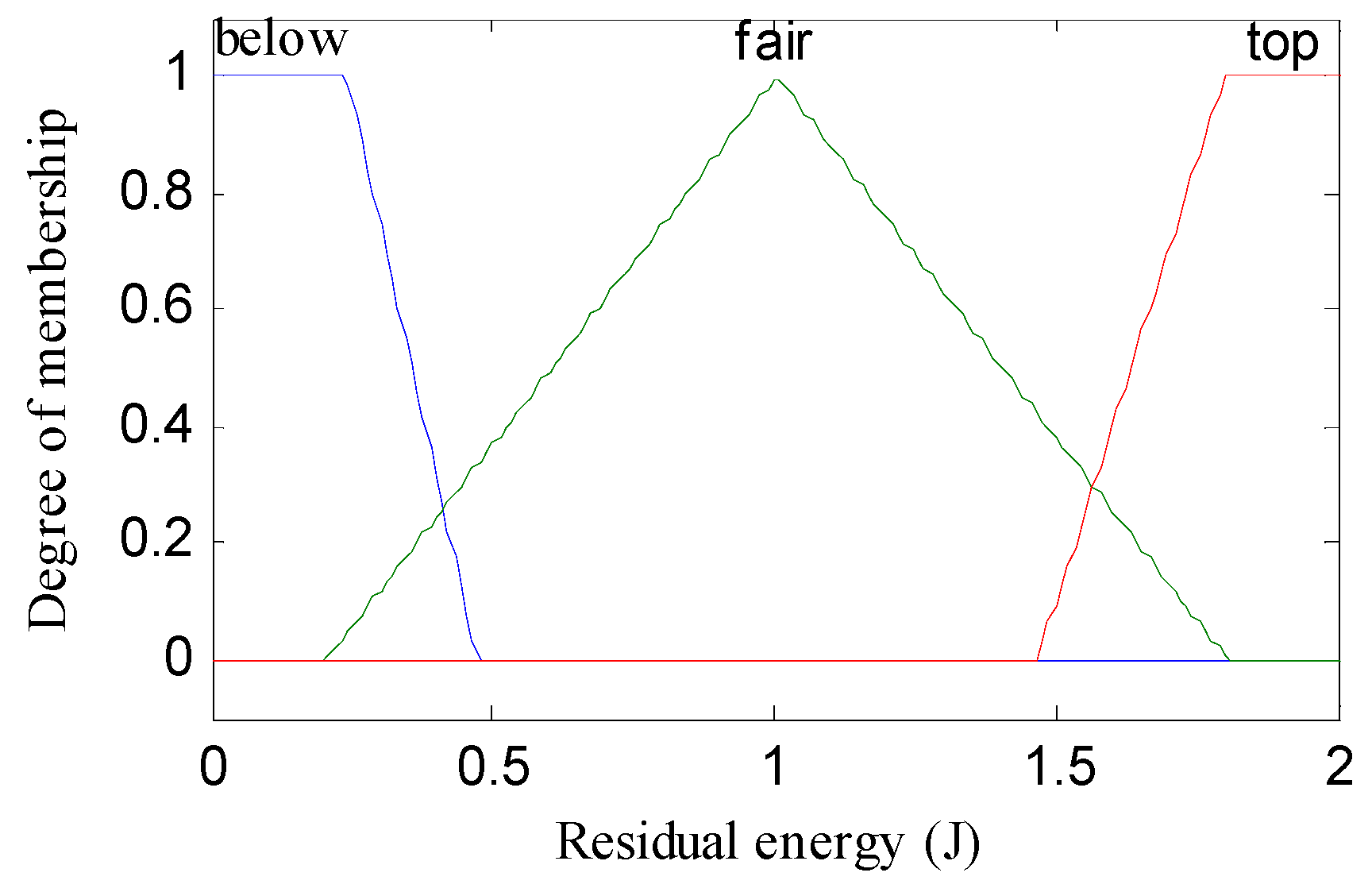
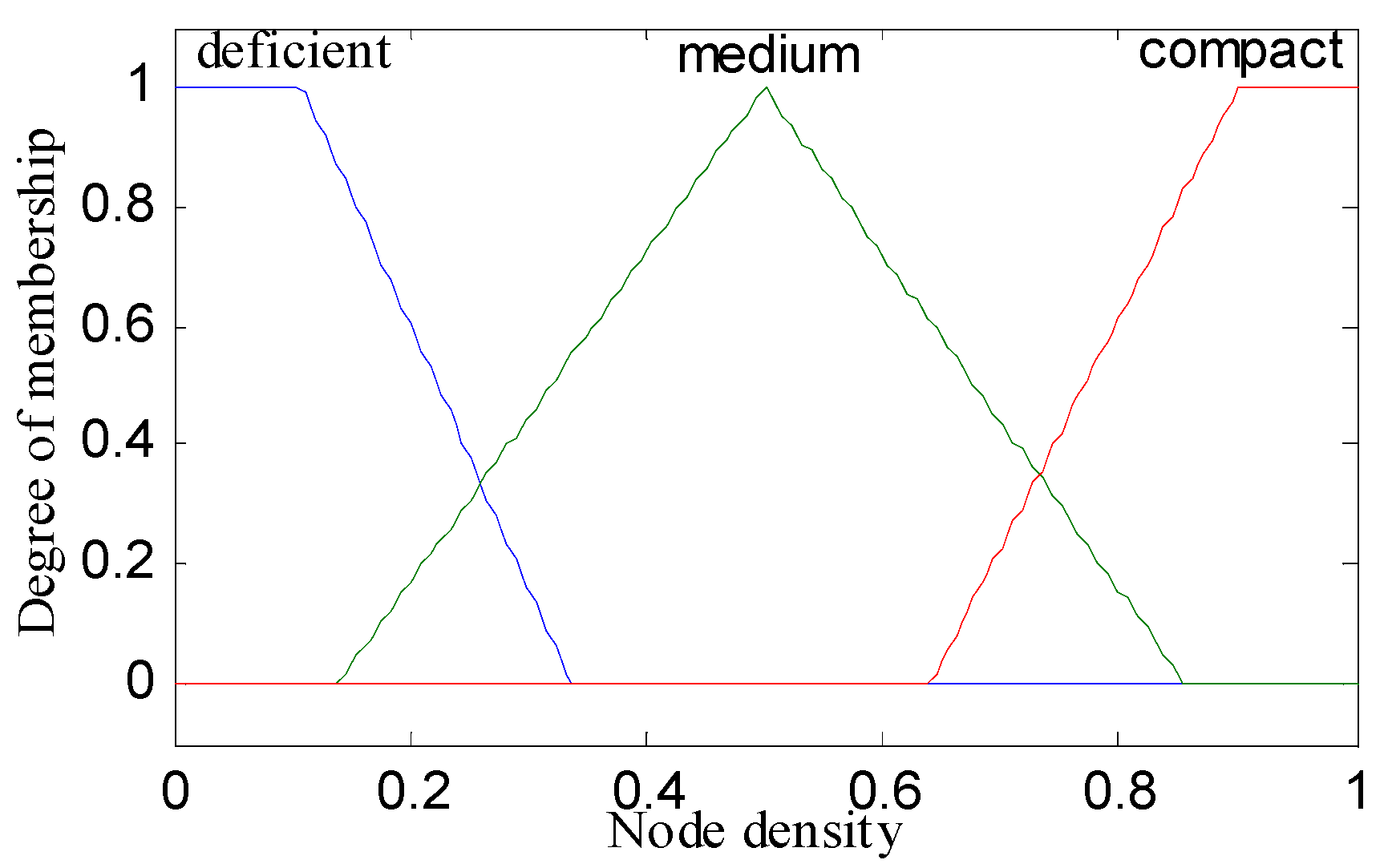
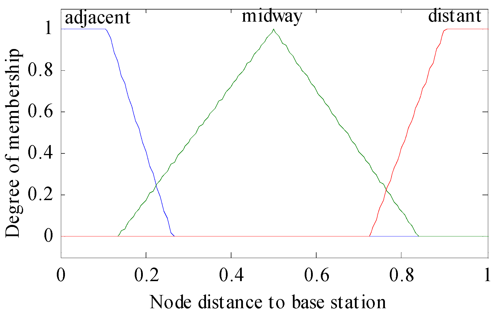
  • Fuzzification or Input Crisp Value: In this step, we input the three metrics: residual energy, node density, and distance to base station as crisp values in the fuzzy inference system. In this step, the inference system creates membership functions for each metric that is the intersection points.
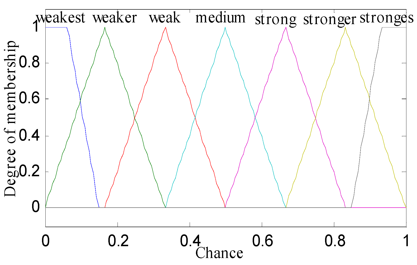
  • Knowledge Base or If–Then Rules: The knowledge base consists of all 27 rules, which runs concurrently on inputs and generates output as chance values. There are multiple inputs (three membership values), but selection is done among the minimum membership values which use fuzzy AND operator.
  • Aggregation: There are 27 rules in the fuzzy inference system, which give multiple outputs. In this step, we aggregate all the output to generate a single fuzzy output set using union fuzzy OR operator which choose maximum of rule evaluation.
  • Defuzzification: In this step, whether a sensor node can act as a cluster head or not is computed. For this purpose, we use a centroid method in the defuzzification step under the fuzzy set to get from aggregation, which is given by Equation (3).
N O D E   C H A N C E   ( C H ) = µ c ( z ) z d y / µ c ( z ) d z
where µ c ( z ) measures the rate of the membership function of the entity z within fuzzy set C , which is described as follows: C = { ( z , µ P ( z ) ) /   z   ϵ   Z , where Z denotes the universe of discourse.

3.2.2. Adaptive Neuro-Fuzzy Inference System

Fuzzy logic and artificial neural networks are good candidates for making smart artificial intelligence systems because of their generalization and non-linearity properties. We developed a hybrid system which consists of two different soft-computing techniques: fuzzy logic and artificial neural networks. We named the hybrid system an adaptive neuro fuzzy inference system (ANFIS). Fuzzy logic has expertise in the area of shapes but not on the subjective aspects of human learning into the procedure of exact quantitative analysis. But in any case, it does not have a characterized technique that can be utilized as a guide during the change from human idea into knowledge or rules-based fuzzy inference systems. It is also requires much time to adjust the membership function. Not at all like artificial neural networks, it has a higher ability in the learning procedure to adjust to its condition. Along these lines, the artificial neural network can be used to consequently alter the membership function and lower the rate of error in the assurance of tenets in fluffy rationale. Artificial neural networks are used for weight adjustment of the membership function of the antecedent and consequent of fuzzy-rule-based systems. Jang [49] proposed the ANFIS, which implements the Takagi–Sugeno fuzzy inference system of five layers. The ANFIS technique was intended to permit membership function and if–then rules to be developed in the light of already acquired data of metrics that are input or output data from the previously designed adaptive fuzzy inference system (AFLIS) in Section 4.1. In addition to the ANFIS, the fuzzy rules are tuned automatically, which is already used in adaptive fuzzy inference systems by using supervised learning. The ANFIS uses a trapezoidal membership function for weight adjustment. These membership functions were used with product inference rules in fuzzification level. The model of the proposed ANFIS with three inputs and one output is shown in Figure 5. Each input used the three membership functions following the Takagi–Sugeno type model containing 27 rules, and each of the nodes were governed by the if–then rules shown in Table 1. The antecedent part of the rules depicts a fuzzy subspace, whereas the subsequent part determines the output inside the fuzzy subspace.
The ANFIS system is a feed-forward neural network with five layers using a supervised learning algorithm. These layers are denoted as fuzzy layer, T-norm layer, normalized layer, defuzzy layer, and aggregated layer, which represent the first, second, third, fourth, and fifth layers, respectively. The first and fourth layers have adaptive nodes, and the remaining layers have fixed nodes. There are three inputs: residual energy (RE), node distance to base station (NDBS), and node density (ND), and one output: chance (CH). We developed twenty-seven rules of “if–then” for the proposed ANFIS system based on the Takagi–Sugeno fuzzy inference model. These rules are
Rule 1 = If RE is below, NDBS is adjacent and ND is deficientThen F 1 = S1m + T1n + U1o + P1
Rule 2 = If RE is below, NDBS is adjacent and ND is mediumThen F 2 = S2m + T2n + U2o + P2
Rule 3 = If RE is below, NDBS is adjacent and ND is compactThen F 3 = S3m + T3n + U3o + P3
Rule 25 = If RE is top, NDBS is distant and ND is deficientThen F 25 = S25m + T25n + U25o + P25
Rule 26 = If RE is top, NDBS is distant and ND is mediumThen F 26 = S26m + T26n + U26o + P26
Rule 27 = If RE is top, NDBS is distant and ND is compactThen F 27 = S27m + T27n + U27o + P27
where below, adjacent, and deficient are the membership functions or linguistic variables of inputs RE, NDBS, and ND (part of antecedent), respectively, and Si, Tj, U k are linear parameters of then part (consequent) of the Takagi–Sugeno fuzzy inference model. The linguistic variable for residual energy RE (M) = (below, fair, top) is represented as (M1, M2, M3), node distance to base station NDBS (N) = (adjacent, midway, distant) is represented as (N1, N2, N3) and node density ND (O) = (deficient, medium, compact) is represented as (O1, O2, O3).
1. 
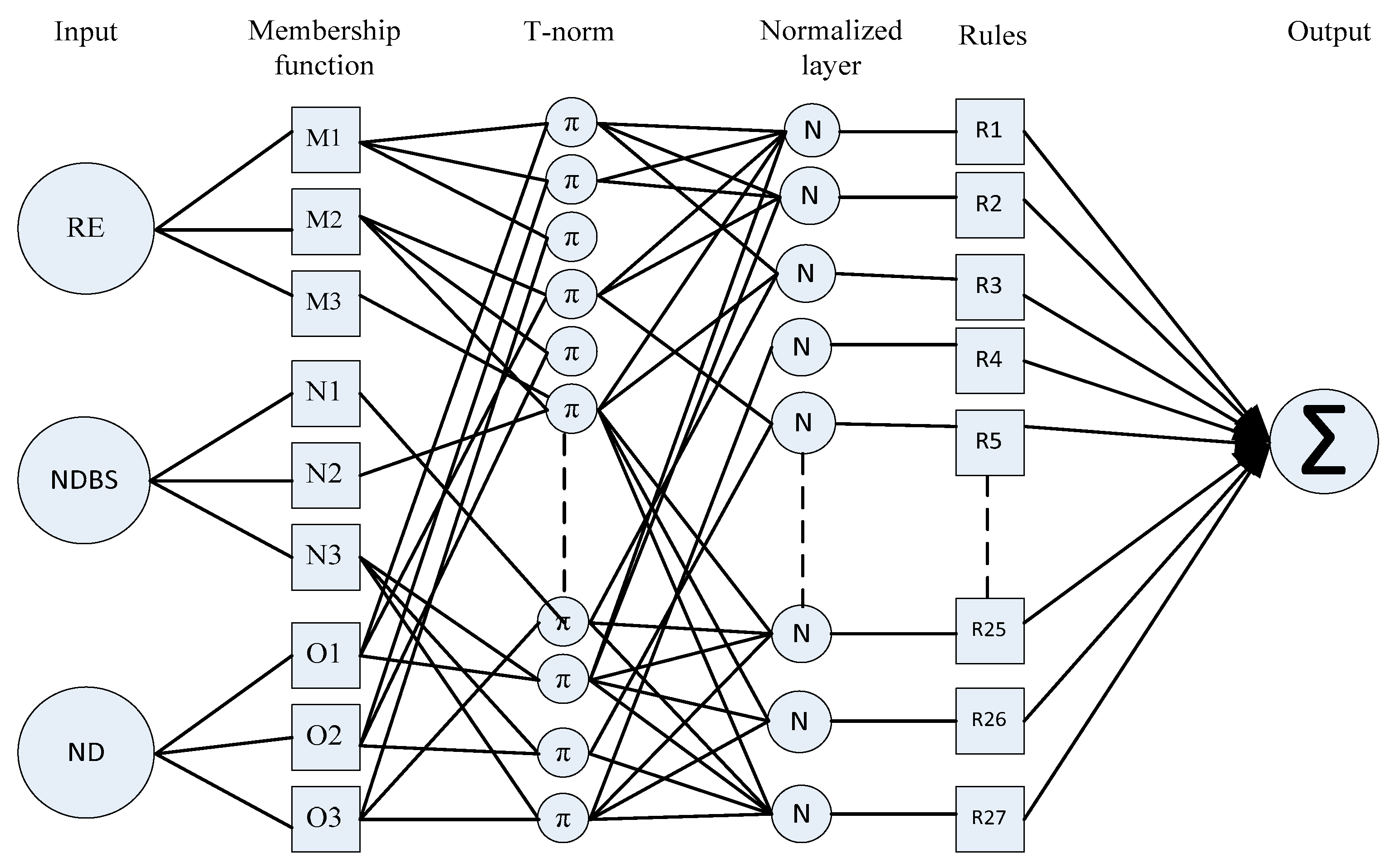
Fuzzy Layer: This section describes the nature of the node which is actually flexible according to backward pass (denoted by square adaptable node) that resembles each input variable relative to membership function. The membership function graph is plotted against each adaptable node to describe their output. Membership function follows Gaussian distribution as shown in Equation (4) or generalized bell-shaped membership function (see Equation (5)) which gives a value in the range of 0 and 1.
μ M α ( M ) = e x p [ ( m f α 2 d α ) 2 ]
μ M α ( M ) = 1 1 + | m f α d | 2 e α
The output of the first layer is given by
  •   R 1 , α = μ M α ( M ) ,   α = 1 , 2 , 3
  • R 1 , α = μ N α ( N ) ,   α = 1 , 2 , 3
  • R 1 , α = μ O α ( O ) ,   α = 1 , 2 , 3
where M is the input node to α and μ M i ,   μ N i ,   μ O i are the degree of membership function cross-ponding to linguistic variables M i , N i , and O i and { d i , e i , f i } are referred to as a parameter set of the membership function or premise parameter. The bell-shaped membership function varies along with the values of the premise parameter set. In this layer, we can also use the triangular and trapezoidal membership function for the input node; they are also valid quantifiers for this node.
2. 
T-Norm Layer: In this layer, each node is non-adaptive in nature, and called as rule nodes which are depicted by the circle labeled with π (see Figure 5). These nodes represent the firing strength of each rule connected to it. To determine the results of each node, multiply all the signals (membership function) coming to the node. The T-norm operator uses generalized AND to calculate the antecedents/outputs at second layer of the rule.
R 2 α = T α = μ M α ( M ) μ N α ( N ) μ O α ( O ) ,   α = 1 , 2 , 3
where T α is the output of each node which stands for each rule’s firing strength.
3. 
Normalized Layer: Non-adaptive in nature nodes found in the normalized layer, which is known as normalized mode, are depicted by circles labeled as N (see Figure 5). The output of every node is an estimation of the proportion between the α th rule’s firing strength to the summation of firing strength of all rules. The result at the third layer or normalized output can be expressed as
R 3 α = T n α = T α α T α ,   α = 1 , 2 , 3
4. 
Defuzzy Layer: This layer consists of those nodes which have adaptive essence depicted by a square (see Figure 5). The output of the node is the product of normalized firing strength and individual rule. The output at the fourth layer can be given by
R 4 α = T n α   f α = T n α ( s α m + t α n + u α o + p α )
where T n α ( s α m + t α n + u α o + p α ) is the normalized firing strength from the normalized layer and ( s α m + t α n + u α o + p α ) is a parameter in the node. Defuzzy layer parameters are also known as a consequent parameter.
5. 
Aggregated Output Layer: This layer consists of a single consolidated node as an output which is specified as non-adaptive in nature. This non-adaptive node gives information about the complete system performance evaluated by adding up all the approaching signals arriving at this layer from the previous node. Summation sign is used inside a circle to represent this aggregated output node. The output of the fifth layer is computed as
R 5 α = α T n α   f α = α W α f α α w α
The ANFIS uses the adaptive neuro fuzzy clustering algorithm (Algorithm 1) to train the premise and consequent parameters. The first layer resembles the adaptive node, which contains the non-linear premise parameter, and the fourth layer consists of the linear consequent parameters. Initially, the gradient descent or back propagation method is used as a learning algorithm. There may be a chance to stick in local minima and slow convergence rates while using back propagation. To rectify these problems Jang [49] uses a hybrid learning algorithm in which two learning strategies—least mean squares and gradient descent—are merged. The convergence rate of the hybrid learning algorithm is much faster than general artificial neural networks that never include local minima. The working strategy of the ANFCA incorporates two passes: forward pass and backward pass. In the forward pass, input signals (premise metrics) are propagated layer by layer until the fourth layer. These metrics are fixed, and consequent metrics are updated using the least mean squares method. After obtaining the output data at the fourth layer, the data are compared with the actual output and the error is calculated. Now, in the backward pass, the errors which occurred due to the comparison of the output generated in the forward pass and the actual output are sent back to the adaptive node of the first layer. At the same time, the membership functions (premise metrics) are updated using the gradient descent method or back propagation method. During this time, consequent metrics are fixed. Each level of learning is called an epoch. The proposed algorithm works in three phases: selection phase, cluster formation phase, and transfer phase. In the first phase, cluster heads are selected. In the second phase, clusters are formed by calculating their area based upon radius. In the final phase, cluster heads transfer the aggregated data to the base station. The precise description of each phase is presented in the next section.
Algorithm 1- Adaptive Neuro Fuzzy Clustering Algorithm (ANFCA)
1.Begin
2.Input: Given input training pattern, {RE, NDBS, ND} and maximum number of Epoch to Emax. // obtained from first modeling mamdani type fuzzy inference system.
3.Output {CH}
4.Process
5.for E=1 to Emax.
6.  Input the training data into first layer of Takagi-sugeno inference engine.
7.  Membership function μ M α ( M ) tuned using Equations (4) and (5).
8.  Adjust the firing strength of each node ( T α ), using Equation (6) in non-adaptive T-norm layer.
9.  Normalize the firing strength of each node ( W n i ) using Equation (7) in normalized layer.
10.  Defuzzification of each node using Equation (8).
11.  Aggregated output is produced for each node using Equation (9) in fifth layer.
12.END

3.2.3. Phases of the Algorithm

The proposed algorithm of the ANFCA works in three phases as follow.

Selection Phase

Initially, the base station starts the operation of clustering; it broadcasts a beacon message (request for IDs, residual energy, distance to base station, and its density) in the network. All the sensor nodes reply an acknowledgment with requested information. Every node estimates the distance between base station and itself using received signal strength indicator. Equation (10) determines the received signal strength.
S r = S o + 10 β   l o g ( a r a o ) + δ
S r = S o 10 R S S I θ 10 α
where S o (in decibel meter) is the reference signal strength at distance a o , β is used to represent path loss exponent (2 ≤ β ≤ 4), and a r is the actual distance. Gaussian random variable is represented by δ having mean zero and variance σ2 (in decibel meter 4 ≤ σ ≤ 12). The distance between the base station and a node is calculated using Equation (11). Where θ is the received signal strength in one meter distance from the base station without any obstacles. The base station triggers election procedures for cluster heads choosing some nodes as cluster heads randomly. These temporary cluster head nodes are gone through AFLIS to check the validity of each node whether they can play the role of cluster head or not. Afterwards, output of AFLIS is recorded and trained using ANFIS, and the final output is recorded. If the nodes have fulfilled the selection criteria for a cluster head, then these nodes are designated as permanent cluster heads for the present round. The selection procedure for a cluster head is rehashed in each cycle so it is potentially able for the sensor to get opportunity to become a part of cluster head group, therefore all nodes exhaust their energy relatively that upgrades the network lifetime.

Cluster Formation Phase

The ANFCA forms variable sizes of clusters; the cluster head manages the number of nodes or cluster sizes that eventually balances the load with periodic replacement of cluster heads. Initially, selected cluster heads calculate their radius for formation of cluster phase. The mean radius of each cluster head is obtained by the Equation (12)
C r m i n i m u m = A × A π × n × k
whereas n represents the number of nodes deployed inside the network of area A × A , and k represents the number of clusters. Generally, a cluster has at least a radius equal to C r . After radius calculation, each cluster head acquires an area according to their radius then sends a join message to each node within the cluster. The nodes make the decision based upon the received signal strength to join which cluster. The sensor node which does not receive any join message declares themselves as cluster head and sends their data directly to the base station. The nodes within the defined radius are called member nodes for their respective clusters. Now, cluster heads schedule a time-division multiple-access approach to gather data from member nodes. This time-division multiple-access schedule reduces intra-cluster collision in addition to cutting down on energy utilization because of the limit on the number of messages exchanged between member nodes. Each cluster head broadcasts time-division multiple-access schedule information in their clusters to their member nodes on when they are able to send messages to their cluster head. The cluster head dictates the time slot for every node, only in their specific time slot can nodes send their message to the cluster head. Therefore, nodes enter the wake-up mode in their time slot, otherwise they go into sleep mode. In this way, nodes conserve their energy. The cluster heads gather messages from their member nodes and apply data aggregation to form single packets of a fixed size.

Transfer Phase

According to the time-division multiple-access schedule, the cluster head gathers and aggregates data, and then communicates to the base station directly without using any relay node. The number of messages exchanged is limited to the number of cluster heads which reduces the energy consumption.

4. Simulation

In this section, the performance of the proposed adaptive neuro fuzzy clustering algorithm (ANFCA) was analyzed. The proposed algorithm was simulated by writing a script in MATLAB (R2019a, MathWorks, Natick, MA, USA) and using simulator tools: FIS and ANFIS. The simulator FIS consists of a fuzzy inference model and membership function for each considered metric: residual energy, node density, and node distance to the base station. The ANFIS simulator produced the output that determined the cluster head. The proposed algorithm ANFCA was compared with LEACH, fuzzy-logic-based CHEF, and energy prediction technique using fuzzy-logic-based LEACH-ERE to show its effectiveness.

4.1. Simulation Environment

In this section, the simulation parameters used to conduct simulation of the ANFCA are presented. We considered a 200 × 200 node simulation area of the network, where 200 sensor nodes were distributed randomly. The sensing capabilities of the nodes were limited to 5 m and they were allowed to transfer data within a 25-meter range in a symmetric way. The simulation cycle time was approximately 60 µs, and it ran until all nodes had died. The size of the packets were 512 bits. The simulation metrics and their values are shown in Table 2.

Evaluation Metrics

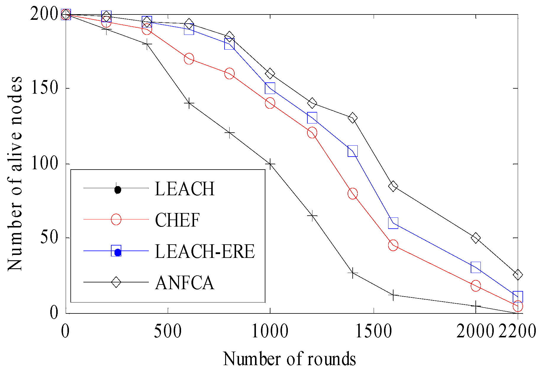
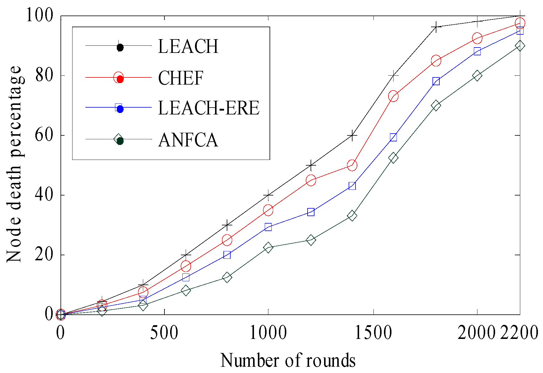
Network Lifetime: Lifetime definition of the network is application dependent, and it may be stated that as the tenure spans from the start, it is the functioning of the network to a moment when a certain percentage of the nodes have died or the network will be disconnected. In this paper, we considered the simulation time until 90% of the nodes were dead.
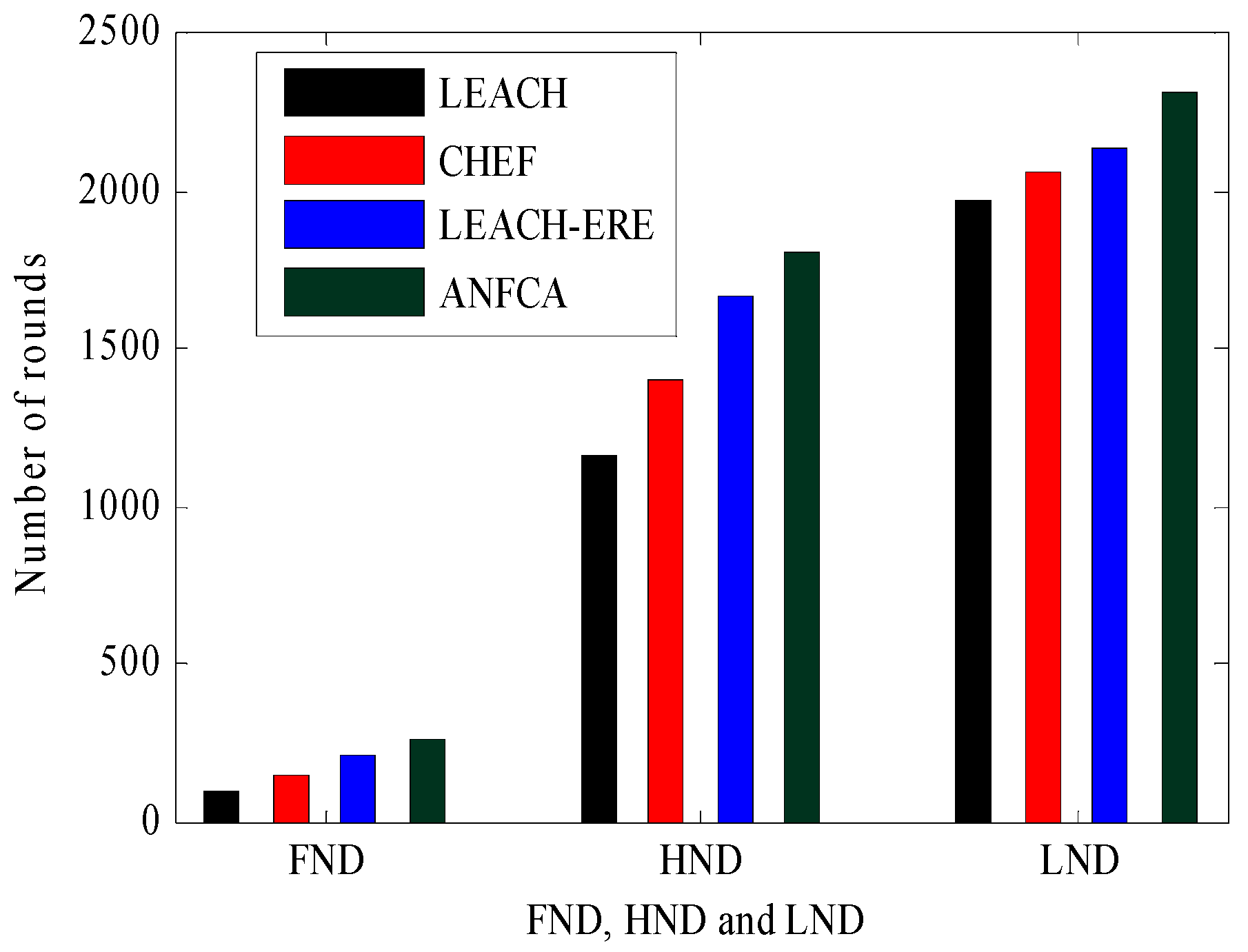
(First node death) FND, (Half node death) HND and (Last node death) LND: The round at which the death of the first node occurred was defined as FND. Similarly, the round at which half of the nodes had died was defined as HND. The round at which the last node death has occurred was taken as LND.
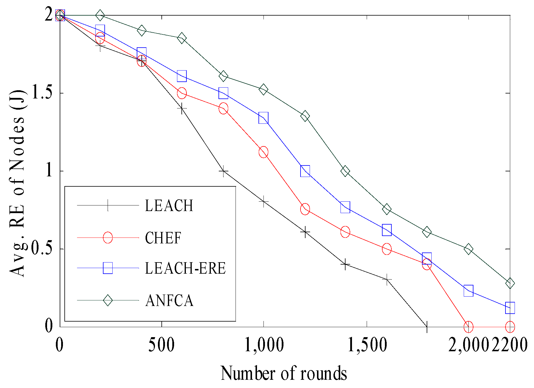
Average Residual Energy: Defined as the mean of residual energy of alive nodes in the network with respect to rounds.
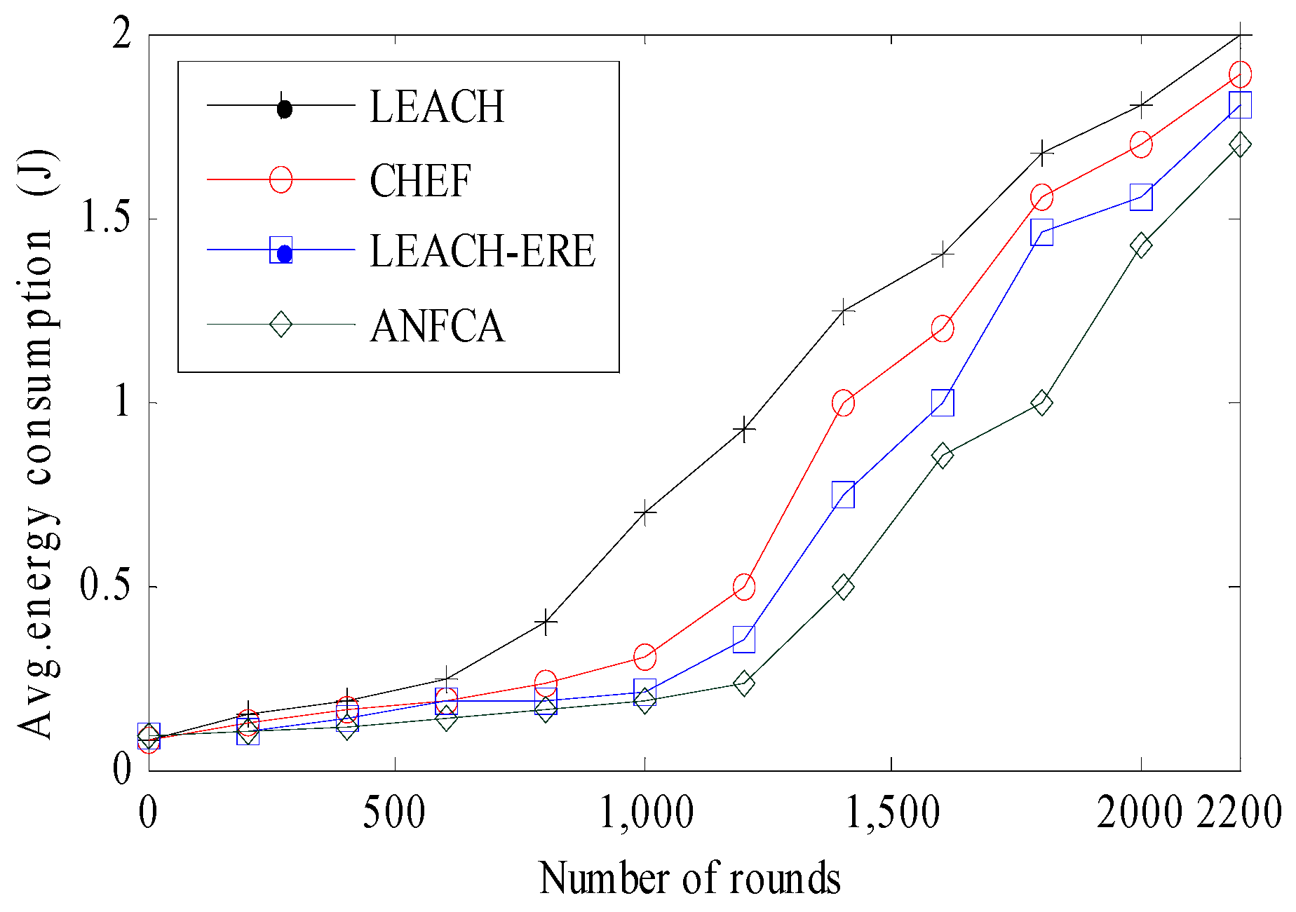
Average Energy Consumption: Defined as the summation of overall energy consumption taken place during the sensing and transmission by each sensor node to the number of sensor nodes with respect to rounds.
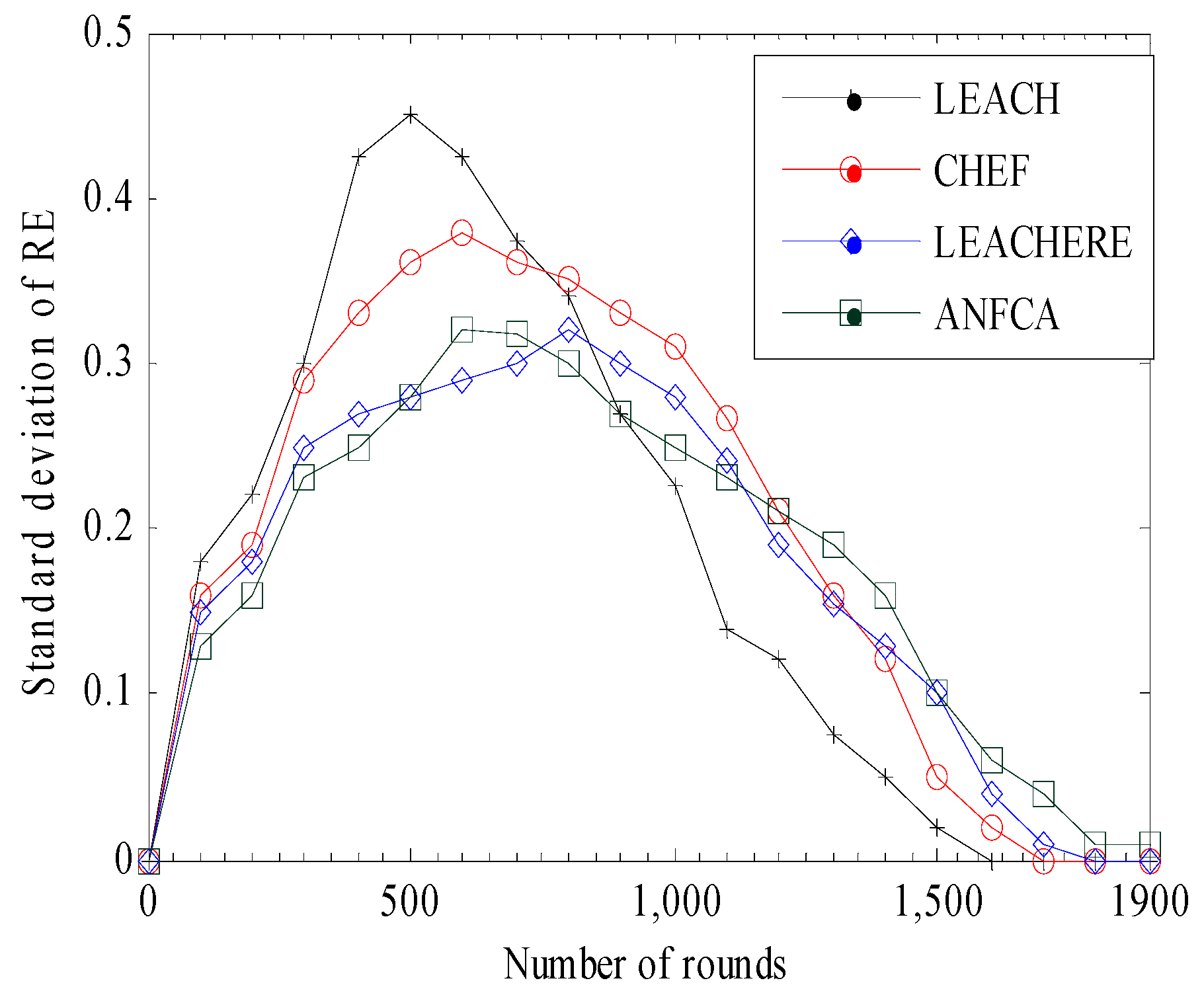
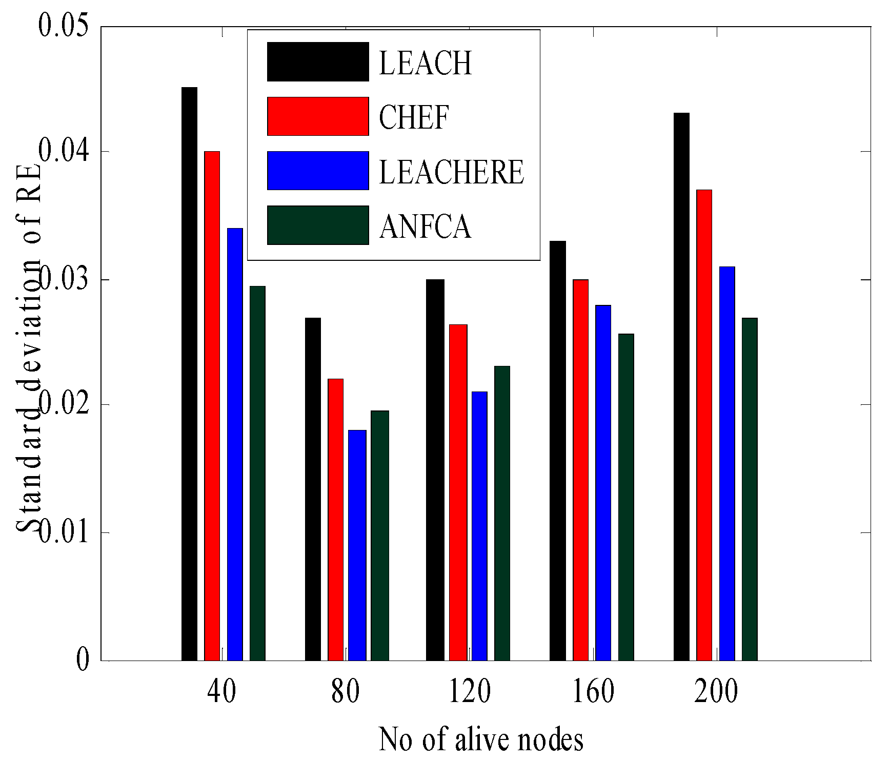
Standard Deviation of Residual Energy: The standard deviation of residual energy is the square root of variance of residual energy of all the sensor nodes. It shows the variation of residual energy around the mean.

4.2. Simulation Results

4.2.1. Network Lifetime Over Rounds

Figure 6 shows the results obtained in the simulation for functioning nodes with respect to each round. It was observed that 90% of all 200 nodes had died by 2000 rounds, and the remaining 10% stretched the lifetime of the network up to another 100 rounds (total: 2100 rounds) for the LEACH algorithm, whereas CHEF showed little improvement over the classical LEACH (20% improvement in network lifetime) which ran up to 2220 rounds smoothly, and there were still 20 nodes alive. The LEACH-ERE initially showed up to 800 rounds with only 20–30 nodes having died, and thereafter the death rate of the nodes increased and almost followed the CHEF curve. The LEACH-ERE showed a 4–5% enhancement over the CHEF and 25% over LEACH. The LEACH-ERE ran up to 2300 rounds. Apart from this proposed algorithm, the ANFCA showed a steady death rate of sensor nodes; at up to 1000 rounds, only 10% of sensor nodes (20 nodes) had died, and thereafter it followed almost a similar curve to the LEACH-ERE up to 1200 rounds. The ANFCA lasted up to 2300 rounds until all 200 sensor nodes (100%) had died. It was clearly observed that the proposed ANFCA runs for a longer time compared with the state-of-the-art algorithms. It is due to the fact that the neuro fuzzy system is employed to rotate the cluster head responsibility among the sensors.
Figure 7 shows the percentage of nodes that died over the increasing number of rounds. From the simulation results, it was observed that the proposed ANFCA does far better than LEACH and LEACH-ERE. Initially, in the LEACH algorithm, the node death percentage rate slowly increased up to 500 rounds, but thereafter there was a sharp drop from 1400 rounds onwards, and all 200 nodes (100%) died before reaching 2200 rounds. In the case of the ANFCA, about 15% more nodes were still alive compared with the LEACH, and 5% of nodes were still alive compared with the LEACH-ERE after completing 2200 rounds, respectively. The rate of node death for the ANFCA was very slow compared to the state-of-the-art algorithms. It is because the proposed algorithm uses a supervised learning approach for the membership function, which is responsible for updating the membership weight function and lowering the energy consumption rate.
Table 3 shows the comparative view of the metrics FND, HND, and LND for the proposed algorithm ANFCA and all of the state-of-the-art algorithms with respect to rounds. Figure 8 shows a comparative view of the death percentages’ connections with FND, HND, and LND for LEACH, CHEF, LEACH-ERE, and ANFCA. It was observed that FND for LEACH was around the 96th round, FND occurred for ANFCA at the 260th round, which was almost two and half times more than that of LEACH, and the last node died at 1970 rounds for LEACH, whereas LND occurred for ANFCA at the 2310th round. Figure 8 and Table 3 show that the proposed algorithm did far better than the state-of-the-art algorithms, and that the lifetime of the network was enhanced because of the lower death rate of the nodes.

4.2.2. Energy Expenditure over Rounds

In this simulation, we show the comparative study of energy expenditure across LEACH, CHEF, LEACH-ERE, and ANFCA. Figure 9 depicts the average residual energy versus the number of rounds for the ANFCA and the state-of-the-art algorithms. Initially, all the sensor nodes had equal energy at 2 joules. The LEACH, CHEF, and LEACH-ERE lost almost equal amounts of energy at 425 rounds, and around 1.72 joule of the average residual energy was remaining out of the initial 2 joules. The energy consumption of the nodes was calculated with the help of Equation (1). The ANFCA outperformed compared to the state-of-the-art algorithms; at the same point (425 rounds), the residual energy of the nodes was approximately 1.86 joule. As the number of rounds increased, LEACH performed the worst among the other algorithms, and all the remaining energy of the nodes was exhausted near 1800 rounds. The CHEF and LEACH-ERE showed better performance than LEACH, in terms of energy usage, with about 11% (up to 2000 rounds) and 20% (up to 2200 rounds), respectively. Overall, in this simulation the proposed algorithm ANFCA did far better than all the other algorithms. The ANFCA ran up to 2480 rounds, and the average remaining residual energy of the nodes was still 0.45 joule.
Figure 10 depicts the average energy consumption versus number of rounds for the ANFCA and the other algorithms. It was observed that, initially, all four algorithms—LEACH, CHEF, LEACH-ERE, and ANFCA—followed the same curvature and consumed almost an equal amount of energy up to 455 rounds, around 0.25 joule. Yet, the ANFCA consumed only 1.67 joule out of 2 joules up to 2200 rounds. In fact, as there was growth in the number of rounds, the LEACH consumed energy much faster than other algorithms because of the probabilistic selection cluster head method and because it does not include the residual energy parameter, whereas CHEF, LEACH-ERE, and ANFCA include fuzzy logic to select a cluster head. The CHEF consumed more energy towards increasing the number of rounds compared with the LEACH-ERE, whereas the proposed algorithm ANFCA showed that the rate of consuming energy by nodes was uniform until the last node death. The ANFCA consumed 10%, 15%, and 40% less energy than LEACH-ERE, CHEF, and LEACH, respectively. This is because cluster head selection is done initially with the AFLIS model, and thereafter it is refined through the selected cluster head ANFIS model. Thus, overall, the ANFCA appears to be energy-efficient, which ultimately enhances the network’s lifetime.

4.2.3. Standard Deviation of Residual Energy

Uniform consumption of energy is highly desirable for load balancing among the sensor nodes which increases the lifetime of the networks. Therefore, we examined the standard deviation of residual energy for all the nodes in the networks and show the variation around the rounds as well as the diaspora from the mean. The energy dissipated by the cluster head and member node per cycle “c” (rounds) was evaluated. The energy consumption by cluster head is expressed as
E d s t c ( h ) = { ( x n 1 ) m E e l e c t + x n m E d a + m E e l e c t + m ε m p f l h   t o   B S 4 , h   ϵ   C H m E e l e c t + m ε f s p l h   t o   B S 2 , h   ϵ   n o n C H
where x n represents the total number of sensor nodes that are actually connected to the cluster head as well as the cluster head node, h is used to represent the nodes, and m is the m -bit data. The average (mean) dissipated energy for a cycle can be computed as
µ ( E d s t ) = h   ϵ   N E d s t c ( h ) N
The residual energy for the next cycle (c + 1) is calculated as
E r e s c + 1 ( h ) = E r e s c ( h ) E d s t c ( h )
The average (mean) residual energy for next cycle is expressed as
µ ( E r e s ) = 1 N i   ϵ   n E r e s c ( h )
The standard deviation of residual energy is the square root of the variance of the residual energy, and is given by
σ ( E r e s d i u a l ) = 1 N i   ϵ   n [ µ ( E r e s ) E r e s ( h ) ] 2
Figure 11 shows the standard deviation of residual energy versus the rounds for all of the algorithms considered in this simulation. The broader the area of standard deviation, the higher the value of a node’s residual energy within one mean (that means that each node dissipates almost equal amounts of energy relatively). The LEACH showed a lower coverage of area among the other algorithms, which means that nodes in the LEACH method have variable amounts of energy dissipation. The CHEF showed much improvement over the LEACH by 27%, as 80% of nodes were within one mean (all 80% had almost equal amounts of residual energy). The LEACH-ERE and the ANFCA were closer to each other on basis of coverage; both the algorithms had coverage of 95% of total nodes. The ANFCA provided a little smoother graph over the LEACH-ERE. For example, as the ANFCA ran up to 2000 rounds, the graph progressed more smoothly. This is because the ANFCA balanced the load using a fuzzy neural system and fairly balanced the energy consumption among the sensor nodes.
Figure 12 shows the alternative representation of the standard deviation of residual energy of functioning nodes for better visualization. As seen from the bar graph in Figure 12, when the number of functioning nodes was 40, the value of the standard deviation for LEACH was 0.045. This was higher than the other state-of-the-art algorithms, whereas the ANFCA had a standard deviation of residual energy equal to 0.027, which means that the load among the nodes was shared fairly in terms of energy consumption. Lowering the value of the standard deviation means a uniform distribution of the load from the mean. That means energy consumption of the load is evenly distributed among the sensor nodes. When the number of alive nodes was between 80 and 120, the values of the standard deviation for the LEACH-ERE was less than the ANFCA. This shows that for lower numbers of nodes, the LEACH-ERE distributed the load more fairly than the proposed algorithm ANFCA, but when the number of nodes increased between 160 and 200, the ANFCA did better than the state-of-the-art algorithms. Lowering the value of the standard deviation of energy means broadening the coverage area, which includes all the sensors nodes within one mean. This shows that the ANFCA has a better capability to distribute the load evenly among the sensor nodes. This is due to the fact that the membership function of residual energy is updated as a result of the role of the cluster head being changed every round among the other sensor nodes.

5. Conclusions and Future Perspectives

Cluster formation in an evenly and energy-efficient manner is of the utmost priority in a sensors-enabled IoT environment. In this paper, an energy-efficient neuro fuzzy hybrid approach for load balancing was proposed. The key components of the ANFCA are an adaptive neural network and a fuzzy logic inference system, which combined the use of residual energy, node distance to base station, and node density to select a cluster head. With the training data of ANFIS from the fuzzy logic system, the membership function and rules can be legitimately tuned to refine the cluster formation process according to the current situation of the network. The results proved that the proposed algorithm ANFCA formulated the evenly distributed clusters, as well as lowered the energy dissipation in the network, which directly improved the network’s lifetime. The simulation results revealed that the proposed algorithm’s performance was one step ahead of LEACH and the fuzzy-logic-based CHEF and LEACH-ERE with regards to cluster formation, energy dissipation, and network lifetime, because ANFCA combined the features of an artificial neural network learning strategy into fuzzy logic. The proposed algorithm could be useful in monitoring in the agriculture field. Our proposed work follows a centralized algorithm where all decisions are made by the base station only. In the future, we plan to extend this work to a distributed algorithm rather than a centralized algorithm, which is suitable for a scalable, fault-tolerant, cluster-based network, which considers RFID-enabled smart sensors with multiple gateways for IoT networks. These multiple gateways are loaded with heavy data, thus it must use distributed approaches to balance the load.

Author Contributions

Conceptualization, P.K.K.; Formal analysis, R.K.; Investigation, P.K.K.; Methodology, P.K.K.; Resources, V.K.; Supervision, S.K.; Writing—review and editing, U.D.

Funding

The research was supported by Jawaharlal Nehru University, New Delhi, India, under the grant DST-PURSE-II Programme.

Acknowledgments

The research was supported by Jawaharlal Nehru University, New Delhi, India, under the grant DST PURSE-II Programme.

Conflicts of Interest

The authors declare no conflict of interest.

References

  1. Farhan, L.; Kharel, R.; Kaiwartya, O.; Hammoudeh, M.; Adebisi, B. Towards green computing for Internet of things: Energy oriented path and message scheduling approach. Sustain. Cities Soc. 2018, 38, 195–204. [Google Scholar] [CrossRef]
  2. Aliyu, A.; Abdullah, A.H.; Kaiwartya, O.; Cao, Y.; Lloret, J.; Aslam, N.; Joda, U.M. Towards video streaming in IoT Environments: Vehicular communication perspective. Comput. Commun. 2018, 118, 93–119. [Google Scholar] [CrossRef]
  3. Kaiwartya, O.; Abdullah, A.H.; Cao, Y.; Altameem, A.; Prasad, M.; Lin, C.T.; Liu, X. Internet of Vehicles: Motivation, Layered Architecture, Network Model, Challenges, and Future Aspects. IEEE Access 2016, 4, 5356–5373. [Google Scholar] [CrossRef]
  4. Kumar, K.; Kumar, S.; Kaiwartya, O.; Cao, Y.; Lloret, J.; Aslam, N. Cross-Layer Energy Optimization for IoT Environments: Technical Advances and Opportunities. Energies 2017, 10, 2073. [Google Scholar] [CrossRef]
  5. Verma, J.K.; Kumar, S.; Kaiwartya, O.; Cao, Y.; Lloret, J.; Katti, C.P.; Kharel, R. Enabling green computing in cloud environments: Network virtualization approach toward 5G support. Trans. Emerg. Telecommun. Technol. 2014, 25, 81–93. [Google Scholar] [CrossRef]
  6. Kaiwartya, O.; Kumar, S.; Lobiyal, D.; Abdullah, A.; Hassan, A. Performance improvement in geographic routing for vehicular Ad Hoc networks. Sensors 2014, 14, 22342–22371. [Google Scholar] [CrossRef] [PubMed]
  7. Ullah, F.; Abdullah, A.; Kaiwartya, O.; Arshad, M. Traffic priority-aware adaptive slot allocation for medium access control protocol in wireless body area network. Computers 2017, 6, 9. [Google Scholar] [CrossRef]
  8. Cao, Y.; Yang, S.; Min, G.; Zhang, X.; Song, H.; Kaiwartya, O.; Aslam, N. A Cost-Efficient Communication Framework for Battery-Switch-Based Electric Vehicle Charging. IEEE Commun. Mag. 2017, 55, 162–169. [Google Scholar] [CrossRef]
  9. Kaiwartya, O.; Kumar, S.; Abdullah, H.A. Analytical model of Deployment Methods for Application of Sensors in non-Hostile Environment. Wireless Pers. Commun. 2017, 97, 1517–1536. [Google Scholar] [CrossRef]
  10. Kaiwartya, O.; Abdullah, A.H.; Cao, Y.; Raw, R.S.; Kumar, S.; Lobiyal, D.K.; Isnin, I.F.; Liu, X.; Shah, R.R. T-MQM: Testbed-Based Multi-Metric Quality Measurement of Sensor Deployment for Precision Agriculture—A Case Study. IEEE Sens. J. 2016, 16, 8649–8664. [Google Scholar] [CrossRef]
  11. Dohare, U.; Lobiyal, D.K.; Kumar, S. Energy balanced model for lifetime maximization in randomly distributed wireless sensor networks. Wireless Pers. Commun. 2014, 78, 407–428. [Google Scholar] [CrossRef]
  12. Aanchal, Kumar, S.; Kaiwartya, O.; Abdullah, A.H. Green computing for wireless sensor networks: Optimization and Huffman coding approach. Peer-to-Peer Netw. Appl. 2017, 10, 592–609. [Google Scholar] [CrossRef]
  13. Liu, A.-F.; Zhang, P.-H.; Chen, Z.-G. Theoretical analysis of the lifetime and energy hole in cluster based wireless sensor networks. Journal of parallel and distributed computing. J. Parallel Distrib. Comput. 2011, 71, 1327–1355. [Google Scholar] [CrossRef]
  14. Khasawneh, A.; Latiff, M.; Kaiwartya, O.; Chizari, H. Next forwarding node selection in underwater wireless sensor networks (UWSNs): Techniques and challenges. Information 2016, 8, 3. [Google Scholar] [CrossRef]
  15. Khatri, A.; Kumar, S.; Kaiwartya, O.; Aslam, N.; Meena, N.; Abdullah, A.H. Towards green computing in wireless sensor networks: Controlled mobility–aided balanced tree approach. Int. J. Commun. Syst. 2017, 31, e3463. [Google Scholar] [CrossRef]
  16. Zadeh, L.A. Fuzzy sets. Inf. Control 1965, 8, 338–353. [Google Scholar] [CrossRef]
  17. Takagi, T.; Sugeno, M. Fuzzy identification of systems and its applications to’ modeling and control. IEEE Trans. Syst. Man Cybern. 1985, 15, 116–132. [Google Scholar] [CrossRef]
  18. McCulloch, W.S.; Pitts, W.H. A logical calculus of the ideas immanent in nervous activity. Bull. Math. Biophys. 1943, 5, 115–133. [Google Scholar] [CrossRef]
  19. Rosenblatt, F. The Perceptron: A Probabilistic Model for Information Storage and Organization in the Brain. Psychol. Rev. 1958, 65, 386–408. [Google Scholar] [CrossRef]
  20. Rosenblatt, F. Principles of Neurodynamics; Perceptrons and the Theory of Brain Mechanisms; Spartan Books: Washington, DC, USA, 1962; Available online: https://catalog.hathitrust.org/Record/000203591 (accessed on 21 February 2019).
  21. Rosenblatt, F. On the Convergence of Reinforcement Procedures in Simple Perceptron; Cornell Aeronautical Laboratory: Buffalo, NY, USA, 1960. [Google Scholar]
  22. Widrow, B.; Lehr, M.A. 30 years of adaptive neural networks: perceptron, Madaline, and back propagation. Proc. IEEE 1990, 78, 1415–1442. [Google Scholar] [CrossRef]
  23. Widrow, B.; Winter, R.G.; Baxter, R.A. Layered neural nets for pattern recognition. IEEE Trans. Acoust. Speech Signal Process. 1988, 36, 1109–1118. [Google Scholar] [CrossRef]
  24. Winter, R.; Widrow, B. MADALINE RULE II: A training algorithm for neural networks. In Proceedings of the IEEE 1988 International Conference on Neural Networks, San Diego, CA, USA, 24–27 July 1988; pp. 401–408. [Google Scholar]
  25. Lin, C.-T.; Lee, C.S.G. Neural-network-based fuzzy logic control and decision system. IEEE Trans. Comput. 1991, 40, 1320–1336. [Google Scholar] [CrossRef]
  26. Berenji, H.R.; Khedkar, P. Learning and tuning fuzzy logic controllers through reinforcements. IEEE Trans. Neural Netw. 1992, 3, 724–740. [Google Scholar] [CrossRef]
  27. Nauck, D.; Kruse, R. Neuro-Fuzzy Systems for Function Approximation. Fuzzy Sets Syst. 1999, 101, 261–271. [Google Scholar] [CrossRef]
  28. Lin, C.-T. FALCON: A fuzzy adaptive learning control network. In NAFIPS/IFIS/NASA ′94, Proceedings of the First International Joint Conference of The North American Fuzzy Information Processing Society Biannual Conference. The Industrial Fuzzy Control and Intellige, San Antonio, TX, USA, 18–21 December 1994; IEEE: Piscataway, NJ, USA; pp. 228–232.
  29. Tano, S.; Oyama, T.; Arnold, T. Deep Combination of Fuzzy Inference. Fuzzy Sets Syst. 1996, 8, 338–353. [Google Scholar]
  30. Juang, C.F.; Lin, C.-T. An online self-constructing neural fuzzy inference network and its applications. IEEE Trans. Fuzzy Syst. 1998, 6, 12–32. [Google Scholar] [CrossRef]
  31. Figueiredo, M.; Gomide, F. Design of fuzzy systems using neuro fuzzy networks. IEEE Trans. Neural Netw. 1999, 10, 815–827. [Google Scholar] [CrossRef]
  32. Nauck, D.; Kalwon, F.; Kruse, R. Foundation of Neuro-Fuzzy Systems; John Wiley & Sons, Inc.: New York, NY, USA, 1997. [Google Scholar]
  33. Jang, R. Neuro-Fuzzy Modeling: Architectures, Analysis and Application. Ph.D. Thesis, University of California, Berkley, CA, USA, July 1992. [Google Scholar]
  34. Heinzelman, W.R.; Chandrakasan, A.; Balakrishnan, H. Energy efficient communication protocol for wireless micro sensor networks. In Proceedings of the 33rd Annual Hawaii International Conference on System Sciences, Maui, HI, USA, 7 January 2000; pp. 3005–3014. [Google Scholar]
  35. Heinzelman, W.B.; Chandrakasan, A.P.; Balakrishnan, H. An application-specific protocol architecture for wireless micro sensor networks. IEEE Trans. Wirel. Commun. 2002, 1, 660–670. [Google Scholar] [CrossRef]
  36. Younis, O.; Fahmy, S. HEED: A Hybrid, Energy Efficient, Distributed clustering approach for Ad Hoc sensor networks. IEEE Trans. Mobile Comput. 2004, 3, 366–379. [Google Scholar] [CrossRef]
  37. Lindsey, S.; Raghavendra, C.S. PEGASIS: Power efficient gathering in sensor information systems. In Proceedings of the IEEE Aerospace Conference, Big Sky, MT, USA, 9–16 March 2002; pp. 1125–1130. [Google Scholar]
  38. Sampalli, S.; Riordan, D.; Gupta, I. Cluster-head election using fuzzy logic for wireless sensor networks. In Proceedings of the 3rd Annual Communication Networks and Services Research Conference, Halifax, NS, Canada, May 2005. [Google Scholar]
  39. Kim, J.; Park, S.; Han, Y.; Chung, T. CHEF: Cluster head election mechanism using fuzzy logic in wireless sensor networks. In Proceedings of the 2008 10th International Conference on Advanced Communication Technology, Gangwon-Do, Korea, 17–20 February 2008; pp. 654–659. [Google Scholar]
  40. Ran, G.; Zhang, H.; Gong, S. Improving on LEACH protocol of wireless sensor networks using fuzzy logic. J. Inf. Comput. Sci. 2010, 7, 767–775. [Google Scholar]
  41. Lee, J.S.; Cheng, W.L. Fuzzy-Logic-Based Clustering Approach for Wireless Sensor Networks Using Energy Predication. IEEE Sens. J. 2012, 12, 2891–2897. [Google Scholar] [CrossRef]
  42. Nayak, P.; Devulapalli, A. A Fuzzy Logic-Based Clustering Algorithm for WSN to Extend the Network Lifetime. IEEE Sens. J. 2016, 16, 137–144. [Google Scholar] [CrossRef]
  43. Nayak, P.; Anurag, D.; Bhargavi, V.V.N.A. Fuzzy based method super cluster head election for wireless sensor network with mobile base station (FM-SCHM). In Proceedings of the 2nd International Conference Advance Computational Methodology; 2013; pp. 422–427. [Google Scholar]
  44. Abidoye, A.P.; Obagbuwa, I.C. Models for integrating wireless sensor networks into the Internet of Things. IET Wirel. Sens. Syst. 2017, 7, 65–72. [Google Scholar] [CrossRef]
  45. Li, Y.; Sun, Z.; Han, L.; Mei, N. Fuzzy Comprehensive Evaluation Method for Energy Management Systems Based on an Internet of Things. IEEE Access 2017, 5, 21312–21322. [Google Scholar] [CrossRef]
  46. Kasana, R.; Kumar, S.; Kaiwartya, O.; Kharel, R.; Lloret, J.; Aslam, N.; Wang, T. Fuzzy-Based Channel Selection for Location Oriented Services in Multichannel VCPS Environments. IEEE Internet Things J. 2018, 5, 4642–4651. [Google Scholar] [CrossRef]
  47. Hu, Q.; Wu, C.; Zhao, X.; Chen, X.; Ji, Y.; Yoshinaga, T. Vehicular Multi-Access Edge Computing With Licensed Sub-6 GHz, IEEE 802.11p and mmWave. IEEE Access 2018, 6, 1995–2004. [Google Scholar] [CrossRef]
  48. Kaiwartya, O.; Abdullah, A.H.; Cao, Y.; Lloret, J.; Kumar, S.; Shah, R.R.; Prasad, M.; Prakash, S. Virtualization in wireless sensor networks: Fault tolerant embedding for internet of things. IEEE Internet Things J. 2018, 5, 571–580. [Google Scholar] [CrossRef]
  49. Jang, J.S.R. ANFIS: adaptive-network-based fuzzy inference system. IEEE Trans. Syst. Man Cybern. 1993, 23, 665–685. [Google Scholar] [CrossRef]
Figure 1. Membership function of RE (residual energy).
Electronics 08 00384 g001
Figure 2. Membership function of NDBS (node distance to the base station).
Electronics 08 00384 g002
Figure 3. Membership function of ND (node density).
Electronics 08 00384 g003
Figure 4. Membership function of CH (chance).
Electronics 08 00384 g004
Figure 5. Three input type-3 adaptive neuro fuzzy inference system (ANFIS) with 27 rules and one output.
Electronics 08 00384 g005
Figure 6. Number of functioning nodes over the rounds.
Electronics 08 00384 g006
Figure 7. Node death percentages over the rounds.
Electronics 08 00384 g007
Figure 8. FND, HND, and LND results over the rounds.
Electronics 08 00384 g008
Figure 9. Avgerage residual energy over the rounds.
Electronics 08 00384 g009
Figure 10. Avgerage energy consumed by nodes over the rounds.
Electronics 08 00384 g010
Figure 11. Standard deviation over rounds.
Electronics 08 00384 g011
Figure 12. Standard deviation over alive nodes.
Electronics 08 00384 g012
Table 1. Fuzzy knowledge database rules.
RuleIF           THENRuleIF           THEN
RENDBSNDCHRENDBSNDCH
1.belowadjacentdeficientweakest15.fairmidwaycompactmedium
2.belowadjacentmediumweaker16.fairdistantdeficientweakest
3.belowadjacentcompactweak17.fairdistantmediumweaker
4.belowmidwaydeficientweakest18.fairdistantcompactweaker
5.belowmidwaymediumweakest19.topadjacentdeficientstrong
6.belowmidwaycompactweaker20.topadjacentMediumstronger
7.belowdistantdeficientweaker21.topadjacentcompactstrongest
8.belowdistantmediumweakest22.topmidwaydeficientmedium
9.belowdistantcompactweakest23.topmidwaymediumstrong
10.fairadjacentdeficientweak24.topmidwaycompactstronger
11.fairadjacentmediummedium25.topdistantdeficientstrong
12.fairadjacentcompactstrong26.topdistantmediumstronger
13.fairmidwaydeficientweak27.topdistantcompactstronger
14.fairmidwaymediumweak-----
Table 2. Modeling framework.
MetricsSpecification
Number of nodes200
Rectangular area200 × 200 m2
Node sensing range5 m
Node transmission range25 m
Base station location(200,170)
Packet size m512 bits
Initial Energy2 J
E T D A 5 nJ/bit/message
E T N E 50 nJ/bit
ε f s p 10 pJ/bit/m2
ε m p f 0.0013 pJ/bit/m4
Cycle time60 µs
Table 3. Node death rate percentages up to 2500 rounds.
Death Percentage (%)LEACHCHEFLEACH-EREANFCA
FND96150205260
2060082711071224
40934122315361707
HND1167140016651810
601386163118851972
801600179519942206
LND1970205621402310

