1. Introduction
In the field of array signal processing, traditional direction-of-arrival (DOA) estimation assumes that a target is a point source. As for underwater acoustic detection, due to multipath propagations between a receive array and a target, especially with the reduction of the distance between the target and the receive array, as many parts of the target reflect signals, the spatial scattering characteristics of the target cannot be ignored. The assumptions of point source models are no longer valid, and distributed source models are presented in such conditions [
1]. A distributed source can be regarded as an assembly of point sources which can be called scatterers within a spatial distribution. The shape of spatial distribution is related to geometry and surface property of a target in underwater detection for instance.
Distributed sources are mainly classified as incoherent distributed (ID) and coherent distributed (CD) sources according to the coherence of scatterers. It’s assumed that the scatterers of an ID source are incoherent, while those of a CD source are coherent. According to the spatial distribution dimension, distributed sources can be classified as one-dimensional (1D) distributed source and two-dimensional (2D) distributed source. 2D distributed source assumes scatterers of a target and receive array are not in same plane, which is more general and accordant with practical circumstances. In this paper, CD sources are considered.
Spatial distributions are characterized by deterministic angular signal distribution function (ASDF), which can be generally modeled as Gaussian, uniform and any other distribution. Parameters of ASDF of a 1D CD source consist of nominal angle and angular spread. With more parameters, ASDF of a 2D source is described by nominal azimuth, nominal elevation, azimuth spread and elevation spread. Nominal azimuth and nominal elevation collectively called nominal angles can also be expressed as nominal DOA representing the center of target. Azimuth spread and elevation spread are collectively called angular spreads denoting the spatial extension of target.
As for ID sources, utilizing different array configurations estimators have been proposed in [
2,
3,
4,
5]. As for CD sources, distributed signal parameter estimator (DSPE) [
1], dispersed signal parametric estimation (DISPARE) [
6] and vec-multiple signal classification (vec-MUSIC) [
7] have been developed from the classical point sources estimation technique MUSIC, where parameters are obtained by 2D spectral searching. A MUSIC like approach has been proposed in [
8] for the DOA estimation of CD sources consisting of both circular and noncircular signals. In [
9], another classical point sources estimation technique ESPRIT has been extended for distributed sources, where the total least square-ESPRIT (TLS-ESPRIT) algorithm is used to estimate nominal angles of sources firstly, and then angular spreads are obtained by 1D spectral searching. The authors of [
10] have developed an efficient DSPE algorithm and proposed a generalized beamforming estimator for CD sources in [
11]. Generally, the parameters of CD sources are approximate solutions under the assumption of small angular spreads, the performance of DSPE algorithm is analyzed in [
12]. All these methods are based on 1D CD source models, which assume that scatterers and arrays are in the same plane. However, scatterers and arrays are not in the same plane but in a three-dimensional space practically. Involving more parameters, 2D CD sources estimation problem is more complicated.
Based on DSPE, several spectral searching methods for 2D CD sources have been proposed. In [
13], an algorithm for exponential CD sources has been presented under nested arrays. The authors of [
14] have proposed an estimator for 2D CD sources under L-shape arrays. Several low-complexity algorithms have been presented in [
15,
16,
17,
18,
19,
20] utilizing two closely spaced parallel linear arrays, treble parallel linear arrays and conformal arrays. It is a common characteristic that utilizing rotational invariance relationships derived by Taylor approximation to generalized steering vectors, the nominal elevation and azimuth are solved under ESPRIT or modified propagator framework. The authors of [
21] have proposed a method using a centro-symmetric crossed array, where DOAs are obtained through the symmetric properties of the special array. Utilizing two closely spaced parallel linear arrays and L-shape arrays, two estimators for CD noncircular signals are proposed in [
22,
23] which exhibit better accuracy and resolution compared with circular signals.
Estimation techniques for CD sources mentioned above assume that the sources are incoherent no matter whether they are 1D or 2D sources. In the field of underwater acoustic detection, the general process of detection is by first emitting narrow-band pulse acoustic signal, then receiving the target backscatter signal, whereby target information is obtained the by analyzing the echo. Therefore, different CD sources are considered as coherent, which is more reasonable on account of the coherent multipath characteristics of underwater acoustic channel. Supposing that signals from different CD sources are coherent, sample covariance matrices are rank defect. Thus, subspace-based algorithms [
1,
6,
7,
8,
9,
10,
11,
12,
13,
14] and ESPRIT class algorithms [
15,
16] which are based on eigendecomposition of sample covariance matrices cannot be applied for DOA estimation of distributed sources. Subspace-based algorithms and ESPRIT class algorithms are based on decomposition of covariance matrix. As to the proposed 2D coherent CD sources, the rank of covariance matrix is less than the source number. Thus, signal and noise subspace cannot be obtained correctly by decomposition of covariance matrix. PM class algorithms [
17,
18,
19,
20] based on linear operation of full rank sample covariance matrices are also no longer applicable. Considering signals from different CD sources are coherent, the authors of [
24] proposed a DOA estimator by virtue of Toeplitz operation of sample covariance matrices, which deal with 1D CD sources.
In this paper, considering 2D CD sources to be coherent with each other, 2D coherent CD sources are modelled first. Then, utilizing double parallel linear arrays, the rotational invariance relationships within and between subarrays have been derived under the assumption of small angular spreads. Next, the decoherence of CD sources can be realized by virtue of 2D spatial smoothing of covariance matrices of receive vectors. Afterwards, two estimators for 2D coherent CD sources are proposed. SS-PM method is proposed base on propagator of sample covariance matrix of spatial smoothing, which is constructed according to the rotational invariance relationships between receive vectors of subarrays. SS-ESPRIT method is established on eigendecomposition of sample covariance matrix of spatial smoothing. The presented methods can estimate DOAs of 2D coherent CD sources effectively without peak-searching, angles matching and information of deterministic ASDF. To show the contributions of this paper clearly, the main differences between the state-of-the-art methods and our work are listed as follows
In [
1,
6,
7,
8,
9,
10,
11,
12,
13,
14,
15,
16,
17,
18,
19,
20,
21,
22,
23], CD sources have been regarded as uncorrelated with each other; estimators cannot be applied for CD sources which are correlated. In [
24], though 1D CD sources correlated with each other are discussed, but the general model of coherent CD sources has not been presented. While in this paper, general 2D coherent CD sources is modelled which consider CD sources as correlated according to characteristics of underwater acoustic channel and general process of underwater acoustic detection.
Though decoherence by spatial smoothing is mature technique with respect to point source model [
25], the proof and conclusion are not applicable to 2D coherent CD source model. In this paper, decoherence with respect to 2D coherent CD sources by spatial smoothing is proposed based on parallel linear arrays. According to receive vectors of subarrays expressed by rotational invariance relationships, the covariance matrix of spatial smoothing is obtained and proven to be full rank.
As for the proposed 2D coherent CD sources model, based on double parallel linear arrays, SS-PM method base on propagator of covariance matrix of spatial smoothing and SS-ESPRIT method established on eigendecomposition of covariance matrix of spatial smoothing are proposed and compared.
The paper is organized as follows.
Section 2 introduces the proposed 2D coherent CD sources model and the receive vectors of double parallel linear arrays. In
Section 3, rotational invariance relationships within and between subarrays and expressions of the receive vectors of subarrays are derived; spatial smoothing method and covariance matrix of spatial smoothing are introduced; SS-PM and SS-ESPRIT are detailed. In
Section 4, simulation results are given and discussed. Finally, the conclusion is drawn in
Section 5.
Notations: Scalar variables are denoted by italic letters, while vectors and matrices are denoted by bold letters. E[•] denotes expectation operation. (•)T denotes the transpose. (•)H denotes the Hermitian transpose. (•)+ denotes pseudo-inverse operator. (./) denotes element-wise division operation. angle(•) denotes phase of a complex number.
2. Arrays Configuration and Signal Model
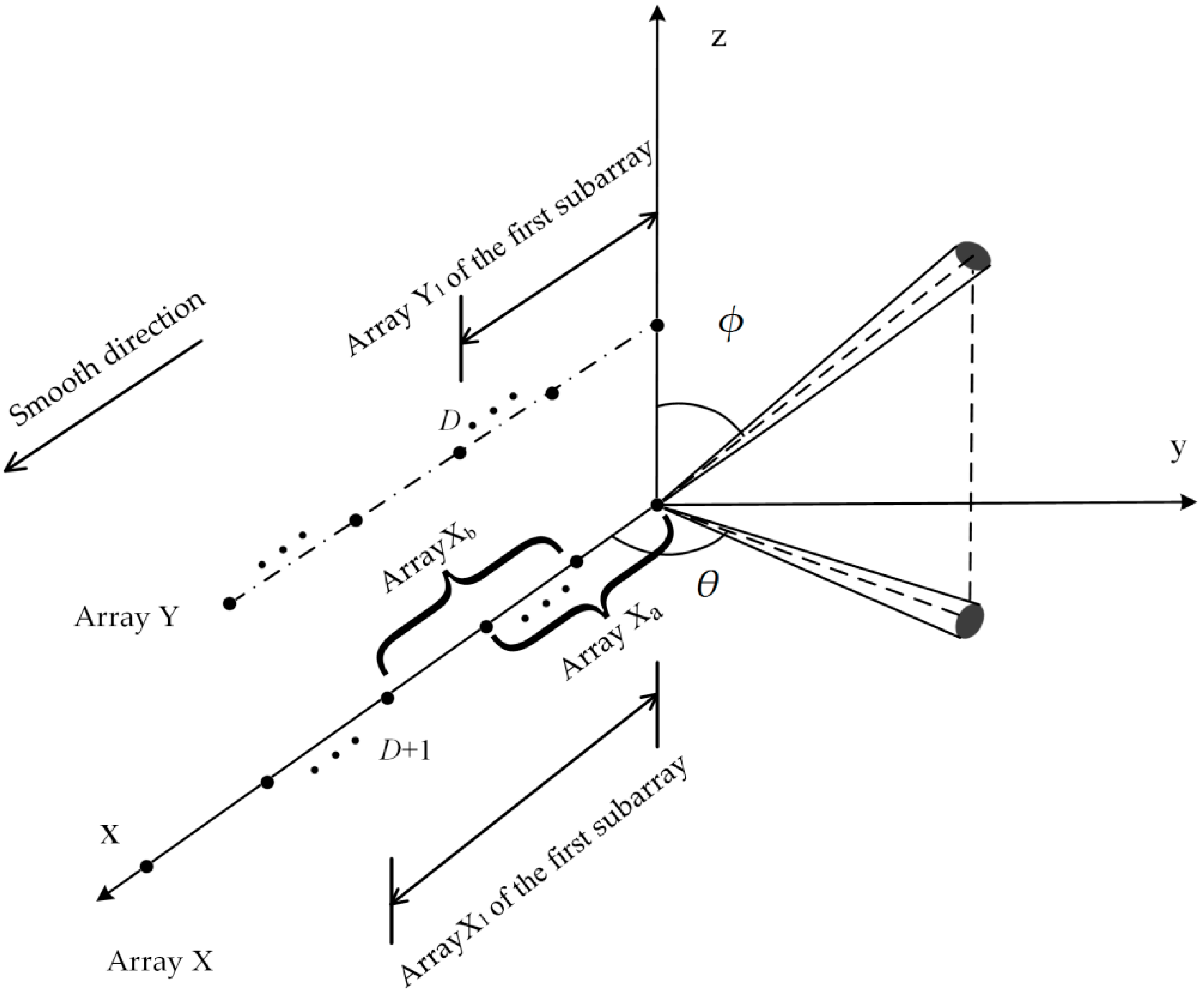
The array configuration is shown in
Figure 1, double parallel linear arrays consist of array X and array Y located on xoz plane. Array X consists of
M sensors on x axis separated by
d meters; array Y parallels to x axis and consists of
M-1 sensors separated by
d meters. The distance between array Y and array X is also
d. It’s assumed that there are
q narrow-band 2D CD sources with wavelength of
λ impinging the array with nominal angles (
θi, φi) (
i = 1, 2, …,
k), where
θi is the nominal azimuth of the
ith CD source,
φi is the nominal elevation of the
ith source,
θi ∈ [0, π],
φi ∈ [0, π]. The noise is assumed to be additive Gaussian white and uncorrelated with signal.
Denote
xk(t) and
yk(t) as the signal received by
kth sensors in arrays X and Y, which can be expressed as follows
where
vi(
t) is the impinging signal to the
ith CD source,
iL is number of scatterers of the
ith source. (
θil, φil) is the azimuth and elevation of the
ilth scatterer of the
ith source. Suppose different scatterers of the same source differ by one phase delay and a random amplitude gain.
αil is complex gain of the
ilth scatterer reflecting the reflection coefficient.
E(
αil) =
αi.
nxk(t) and
nyk(t) are noises received.
Define g(θ,φ;ui) as ASDF which reflects the distribution of scatterers of the ith source. ASDF can be modeled as 2D Gaussian and uniform or any other distribution function. ui = [,,,] is the parameter set of ASDF of the ith source denoting the nominal azimuth, nominal elevation, azimuth spread and elevation spread respectively.
For a Gaussian CD source, deterministic ASDF can be expressed as
For a Uniform CD source, deterministic ASDF can be expressed as
Then
xk(t) and
yk(t) can be expressed as follows (see
Appendix A)
where
si(
t) =
vi(
t)
iLα
i is reflected signal of the
ith CD source. Define
γ(
θ,
φ) are
M × 1 dimensional steering vectors of array X with respect to point source, which can be written as follows
Then the (
M − 1) × 1 dimensional steering vector of array Y with respect to point sources can be written as follows
where
I(M−1)×(M−1) is (
M − 1) × (
M − 1) dimensional identical matrix,
0(M−1)×1 is (
M − 1) × 1 dimensional matrix with all elements as 0.
In the point source model case, steering vectors are used to describe the response of an array. Nevertheless, generalized steering vectors or generalized steering matrices represent the responses of arrays to distribute sources. Generalized signal vectors of array X and array Y reflecting response of arrays to the
ith source can be expressed as follows
Generalized steering matrices of array X and array Y representing response of arrays to all sources can be written as
Thus, the
M × 1 dimensional receive vector of array X and the (
M − 1) × 1 dimensional receive vector of array Y can be expressed as follows
where
s(
t) = [
s1(
t),
s2(
t),
…,
sq(
t)]
T is the signal vector.
nX(
t) and
nY(
t) are the receive noise vectors, which can be expressed as follows
Most CD source models assume that scatterers within a source are coherent, but scatterers between different sources are uncorrelated. According to characteristics of underwater acoustic channel and general process of underwater acoustic detection, supposing signals impinging to different sources are from same emission arrays. Thus, the impinging signals of different sources are correlated and differ by phase delay and a random amplitude gain. Considering the difference between the reflected signal and the imping signals of the
ith CD source lies in a constant complex coefficient
iLα
i, then the signal vector can be written as follows:
where
ρ = [1,
ρ2,
…,
ρq]
T is the coherence coefficient vector,
ρi is the coherence coefficient between the 1th source and the
ith source.
The receive vectors of array X and array Y can be written as
3. Proposed Method
As the proposed 2D coherent CD sources are correlated with each other. The covariance matrices of receive vectors of array X and Y are rank defect. Then traditional estimators established on full rank sample covariance matrices are invalid. Spatial smoothing for 2D coherent CD sources is proposed in this section. This section consists of four parts. First of all, receive vectors of subarrays are expressed with the rotational invariance relationships of generalized steering matrices. Then, covariance matrices of spatial smoothing are derived, which is proved to be full rank. Next SS-PM and SS-ESPRIT methods are proposed. Lastly computational procedure is summarized.
3.1. Subarray Signal Model
As shown in
Figure 1, the first (
D + 1) sensors of array X constitute the array X
1 while the first
D sensors of array Y constitute the array Y
1. Array X
1 and array Y
1 collectively make up the first subarray of the double parallel linear arrays. The receive vectors of the first subarray can be expressed as follows:
where
A1(
θ,
φ) is the generalized steering matrix of array X
1, which actually is the first (
D + 1) rows of
A1(
θ,
φ),
B1(
θ,
φ) is the generalized steering matrix of array Y
1, which is the first
D rows of
B(
θ,
φ).
The space smoothing direction is shown in
Figure 1. Each subarray consists of (
D+1) sensors of array X and
D sensors of array Y. Then the receive vectors of the
pth subarray can be written as
where the generalized steering matrices
Ap(
θ,
φ) and
Bp(
θ,
φ) can be expressed as
As shown in
Figure 1, we define array composed of the first
D sensors in array X
1 as X
a, array composed of the last
D sensors in array X
1 as X
b. The receive vectors of X
a and X
b can be expressed as
where the generalized steering matrices of array X
a and X
b can be expressed as
When the angular spreads of 2D CD sources are small and
d/λ = 1/2, the following rotational invariance relationships can be obtained (see
Appendix B).
where [•]
m is the
mth element of the vector. Rotational invariance relationship of generalized steering matrices within the first subarray can be obtained as
Rotational invariance relationship of generalized steering matrices between the first and the
pth subarray can be obtained as
where
ΦX and
ΦY are the rotational matrices, which can be expressed as
Then the receive vectors of
pth subarray can also be written as
where
Denote
as the power of first CD source
as the power of the noise. The covariance matrix of
pth subarray can be expressed as
Suppose there are
P subarrays within the parallel linear arrays, which means that the subarray can smooth
P times. Then, the covariance matrix of spatial smoothing
R is obtained through taking average of
P covariance matrices of subarrays, which can be written as
where
It can be proven that
R is a full rank matrix when
P ≥
q (see
Appendix C).
3.2. Propagator Method Base on Spatial Smoothing
Combine generalized steering matrices
A1(
θ,
φ) and
B1(
θ,
φ) of the first subarray into
Denote C1 as a matrix of the first qth rows of C and C2 as a matrix of the last (2D + 1 − q)th rows of C. There exists a (2D + 1 − q) × q dimensional propagator operator Ep satisfying C2 = EpC1
Define a (2
D + 1) ×
q dimensional matrix
EDivide
E into three matrices
E1,
E2 and
E3.
E1 selects elements of the first
D rows of
E,
E2 contains elements from 2th to (
D + 1)th rows of
E,
E3 selects elements of last
D rows of
E. We have
From Equations (35) and (36) and rotational invariance relationships described by (25) and (26) we have the following relationship
Covariance matrix of the
pth subarray can be replaced by the sample covariance matrix with
N snapshots, which can be written as
Then the covariance matrix of spatial smoothing can be replaced by
Divide
into
, where
G is the first
qth columns of
and
H is the last (
2D + 1
− q)th columns of
. Then
Ep can be expressed as
Ep . We can obtain eigenvalue
μi (
i = 1, 2, …,
q) and it’s corresponding eigenvectors
ξi of
by means of eigendecomposition of
. From Equations (37) and (38) we can conclude that corresponding eigenvalues of
and
have the same eigenvector; so without angle matching, the eigenvector of
can be obtained as follows
where
11×q is 1 ×
q dimensional vector with all elements as 1. When
d/λ = 1/2, nominal azimuth
θi and nominal elevation
φi can be obtained as follows
3.3. ESPRIT Base on Spatial Smoothing
As the
q ×
q dimensional covariance matrix of spatial smoothing
Rs is full rank, according to Equation (32), we can obtain
. Thus,
Rs is a positive definite Herimitain matrix. Through eigendecomposition, a positive definite Herimitain matrix can be expressed as follows:
where diagonal matrix
Λ =
diag(
ω1,
ω2,…,
ωq).
ωi (
i = 1, 2, …,
q) is eigenvalues of
Rs, which are all positive real number.
F is a
k ×
k dimensional nonsingular matrix. Then
R can be expressed as
From Equation (44), it can be found that through eigendecomposition of
R, there exists a
q ×
q dimensional nonsingular matrix
T satisfying the following relationship:
where
U = [ς
1, ς
2, …, ς
q] is sub-space constituted by eigenvectors of
R corresponding to the
q largest eigenvalues. As both
F and
T are nonsingular matrices,
FT is also a nonsingular matrix. Thus,
U can be divided into
U1,
U2 and
U3.
U1 selects elements of the first
D rows of
U,
U2 contains elements from 2th to (
D + 1)th rows of
U,
U3 selects elements of last
D rows of
U.
According to the invariance rotational relationships described by (25) and (26), we have
Then, the following relationships can be obtained:
As similar to SS-PM, eigenvalue μi (i = 1, 2, …, q) and its corresponding eigenvectors ξi of can be obtained by eigendecomposition of . From Equation (48) we can conclude that corresponding eigenvalues of and have the same eigenvectors; so, the eigenvector of can be obtained from Equation (41). Then, θi and φi can be obtained from Equation (42).
3.4. Computational Procedure Complexity Analysis
Now, procedure of SS-PM can be summarized as follows
Step1: Compute sample covariance matrix of spatial smoothing using Equations (39) and (40).
Step2: Divide into and estimate the propagator operator Ep using Equation Ep . Construct E using Equation (34) and divide E into E1, E2 and E3 from Equation (36).
Step3: Calculate eigenvalue μi (i = 1, 2, …, q) and it’s corresponding eigenvectors ξi through eigendecomposition of .
Step4: Obtain eigenvalue νi of from Equation (41).
Step5: Calculate the nominal azimuth θi and nominal elevation φi from Equation (42).
Procedure of SS-ESPRIT can be summarized as follows
Step1: Compute sample covariance matrix of spatial smoothing using Equations (39) and (40).
Step2: Find the eigenvectors ςi (i = 1, 2, …, q) corresponding to the largest q eigenvectors through eigendecomposition of .
Step3: Constitute sub-space U = [ς1, ς2, …, ςq] and divide U into U1, U2 and U3 from Equation (46).
Step4: Find eigenvalue μi (i = 1, 2, …, q) and it’s corresponding eigenvectors ξi through eigendecomposition of .
Step5: Obtain eigenvalue νi of from Equation (41).
Step6: Calculate the nominal azimuth θi and nominal elevation φi from Equation (42).
The computational complexity of SS-PM includes three parts. Calculation the sample covariance matrix , which is O[PN(2D + 1)2]. Calculation the propagator operator Ep, which is O [q3 + q2(2D + 1) + q(2D + 1)(2D + 1)]. Eigendecomposition of and , which is O(q3). The computational complexity of SS-ESPRIT also mainly includes three parts. Calculation the sample covariance matrix , which is O[PN(2D + 1)2. Eigendecomposition of , which is O[(2D + 1)3]. Eigendecomposition of and , which is O(q3). Obviously, when D > q, the computational complexity of SS-ESPRIT is higher than that of SS-PM.
4. Simulation Results
In this section, five simulation experiments are conducted to verify the effectiveness of the algorithms we proposed. All simulation experiments are based on array configuration shown in
Figure 1. The distance of adjacent sensor
d is set at
λ/2.
denoting root mean squared error (
RMSE) of the
ith source can be expressed as
where
Mc is the Monte Carlo simulations number which is set at 100.
and
is the estimated nominal azimuth and nominal elevation of
ith source in
τth Monte Carlo simulation.
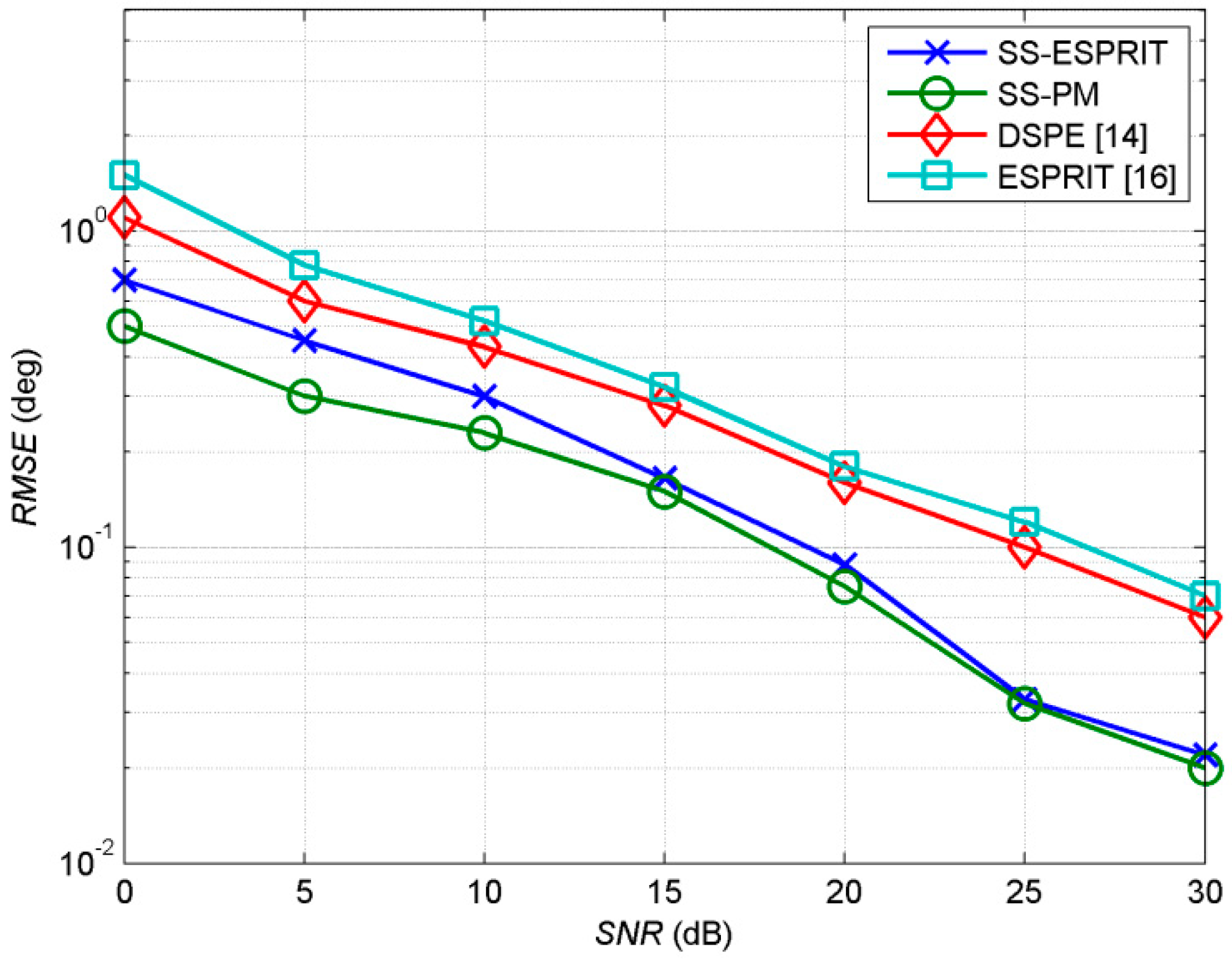
In the first example, we investigate the performance of the proposed methods versus three traditional 2D CD sources which are uncorrelated with each other. The first source is Gaussian CD source with parameter sets [30°, 45°, 2°, 2°]. The second and third sources are uniform with parameter sets [50°, 45°, 2°, 2°] and [50°, 60°, 2°, 2°]. The number of snapshots is set at 400. The sensor number parameter is
D = 4 and the number of subarrays is
P = 4.
RMSE takes the mean
of three sources. Sources are also estimated by DSPE [
14] method using L shaped arrays composed of 7 sensors in both x axis and z axis and ESPRIT [
16] method using double parallel linear arrays with each subarray containing 7 sensors; the distance of adjacent sensor
d are all set at
λ/2. As shown in
Figure 2, the proposed method presents better estimation as
SNR increases. It can be concluded that the proposed method is effective for DOA estimation with respect to traditional 2D CD sources. As utilizing spatial smoothing technique, the proposed two methods shows better performance compared with traditional estimators.
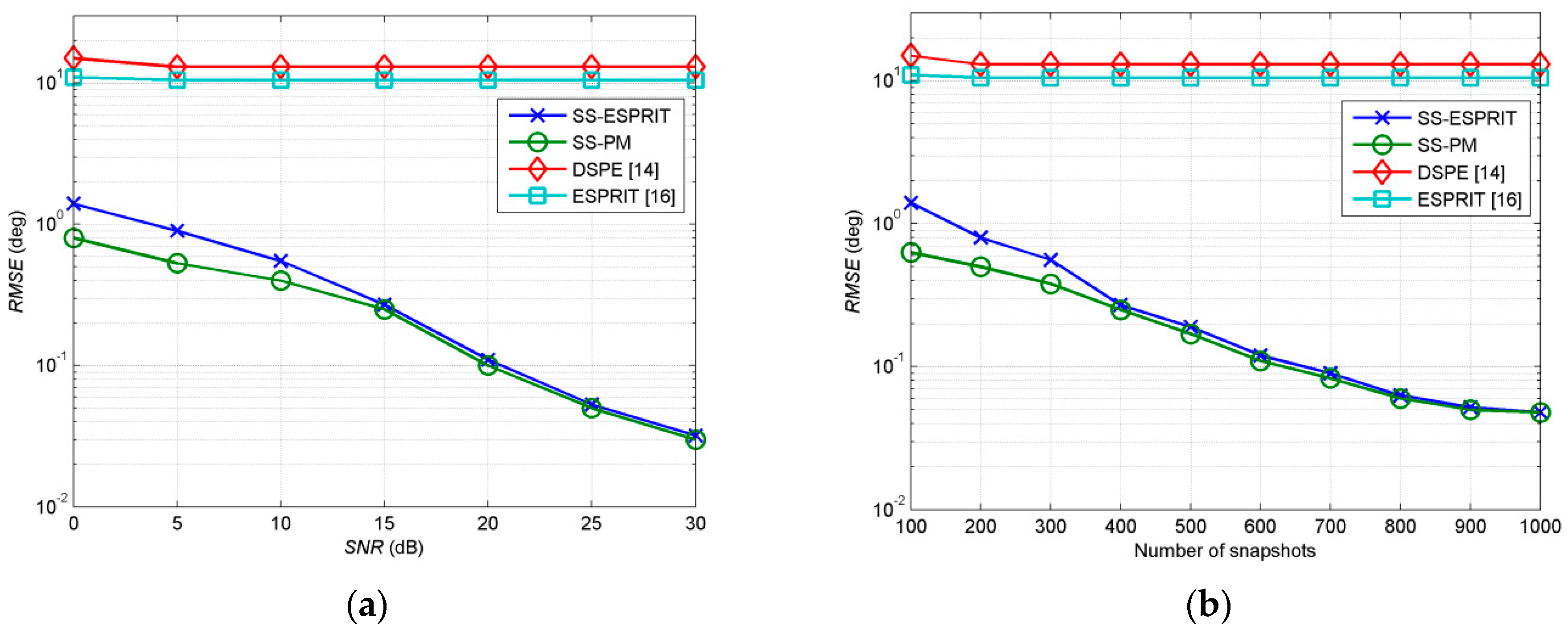
In the second example, we investigate the estimation of the proposed methods for 2D coherent CD sources. We consider two fully coherent sources with equal power. The first source is Gaussian with parameter set [30°, 45°, 2°, 2°]. The second and third source is uniform with parameter sets [50°, 45°, 2°, 2°] and [50°, 60°, 2°, 2°]. The sensor number parameter is
D = 4 and the number of subarrays is
P = 4.
Figure 3a shows estimated
RMSE with
SNR ranging from 0 to 30 dB, while the number of snapshots is set at 400.
Figure 3b shows estimated
RMSE with number of snapshots ranging from 100 to 1000 while
SNR is set at 15 dB.
Figure 3 also show that estimation of the proposed sources by DSPE [
14] and ESPRIT [
16]. As can be seen in
Figure 3, in the case of low
SNR and the lower number of snapshots, the estimation performance of SS-PM is better than SS-ESPRIT. When
SNR and number of snapshots are at low levels, larger errors may exist in eigendecomposition process of sample covariance matrix of spatial smoothing. Thus, SS-PM show better performance than SS-ESPRIT which is based on eigendecomposition. It can be observed that the proposed two algorithms perform better as
SNR or number of snapshots increases. There is no significant difference between SS-ESPRIT and SS-PM when
SNR and number of snapshots are at high levels. Nevertheless, the DSPE [
14] and ESPRIT [
16] present big errors as shown in
Figure 3. As the three CD sources are correlated with each other, the rank of signal subspace is one. DSPE [
14] and ESPRIT [
16] take eigenvector corresponding to the largest eigenvalue as the signal subspace. Both methods can only detect one source, no matter what level the SNR is at. Therefore, errors are big and varieties are not obvious in
Figure 3. It can be concluded that utilizing traditional methods is invalid but SS-ESPRIT and SS-PM are effective for DOA estimation with respect to 2D coherent CD sources.
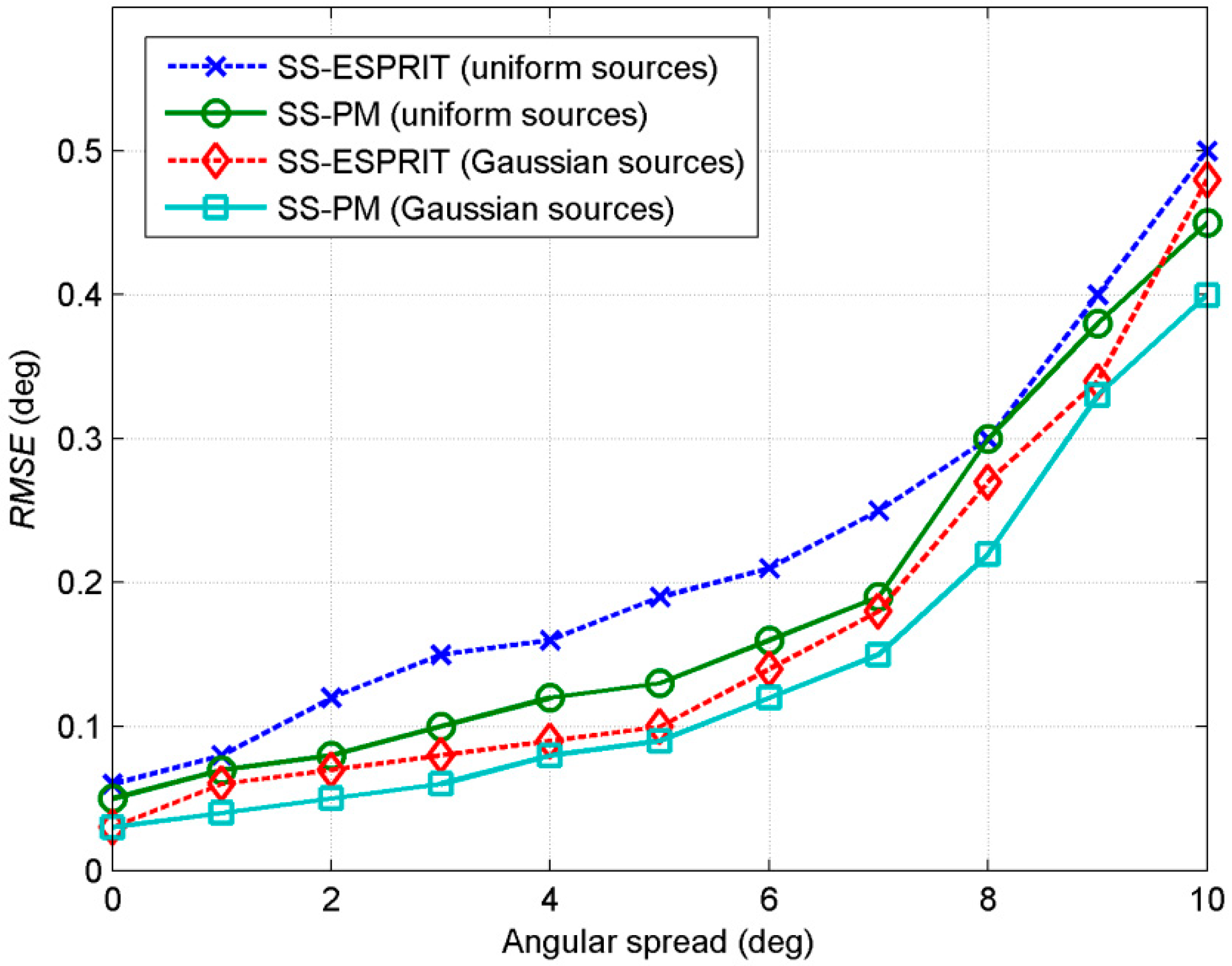
In the third example, we investigate the performance of the proposed methods versus angular spreads. We consider two scenarios. One scenario has two fully coherent Gaussian sources with equal power and the nominal angles are (30°, 45°), and (50°, 60°). The other has two uniform sources with the same nominal angles as the first scenario. To simplify analysis, we assume that azimuth spread is equal to elevation spread in each source and angular spreads of two sources are the same;
σ is used to replace
and
for convenience. The number of snapshots is set at 400 and
SNR is 15 dB.
D = 4 and
P = 4.
RMSE of the two trails is defined as the mean
RMSEi of two sources. From
Figure 4, it can be observed that estimation errors increase as angular spread increase with respect to both Gaussian and uniform sources.
RMSE reaches 0.2° as angular spread increasing to 5°;
RMSE reaches 0.51° as angular spread increasing to 10°. As the receive vector of subarrays are all expressed based on the assumption of small angular spreads. The experiment shows that the two algorithms have satisfactory performance for DOA estimation of 2D coherent CD sources under the condition of small angular spreads
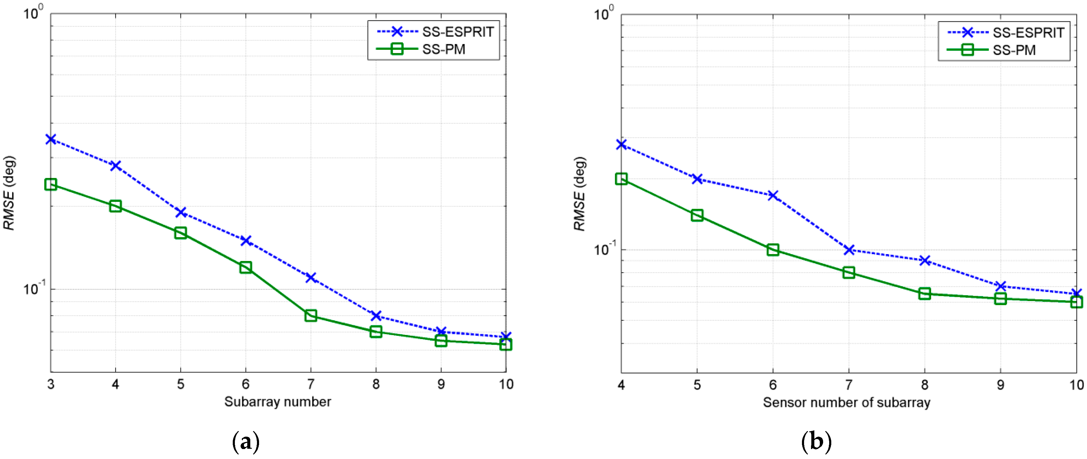
In the fourth example, we investigate the influence of the number of subarrays and sensor number of subarrays on estimation. Considering three fully coherent 2D coherent CD sources with parameter sets as [30°, 45°, 2°, 2°], [70°, 25°, 2°, 3°] and [50°, 60°, 2°, 2°], the first two are uniform and the third one is Gaussian.
RMSE takes the mean
RMSEi of three distribution sources. The experimental settings are as follows: the number of snapshots is 400 and
SNR is 15 dB.
Figure 5a shows the estimation of two algorithms with the number of subarrays varying from 3 to 10 when the sensor number parameter
D = 4.
Figure 5b shows the estimation of the two algorithms with the sensor number parameter of subarrays
D ranging from 4 to 10 while the subarrays number
P is set at 4. The experiment shows that both algorithms can estimate effectively when
D >
q and
P ≥
q. Estimation performance of the two algorithms will be improved with the increasing of the number of subarrays
P when sensor number of subarrays is fixed and the number of subarrays
P is at a low level. As
P increases to a certain extent, the estimation effect will not change significantly. Similarly, the estimation performance of the two algorithms will improve with the increasing of the sensor number of subarrays as the subarrays number
P is fixed, but when the sensor number increases to a certain extent, the improvement of estimation effect is not obvious.
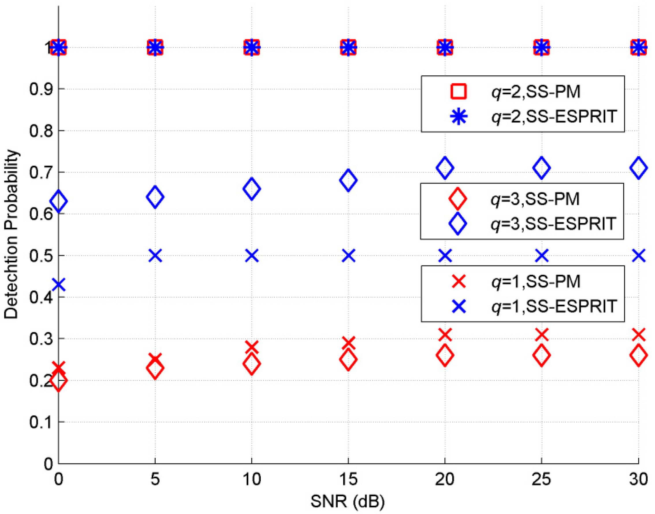
In the fifth experiment, considering both algorithms assume that
q is a priori knowledge, we examine the influence of misestimating of
q on both estimators. For point sources, estimation of the number of sources is a prerequisite for most DOA estimators. When the estimation of the number of sources is wrong, the performance of DOA estimation algorithm will degrade or even fail. Considering point source model, there are some classical estimation algorithms with regard to source number such as information theoretical criterion and minimum description length criterion [
26,
27,
28]. To the best of our knowledge, there are no algorithms of source number estimation for CD sources. Therefor we consider different
q with respect to given number of 2D coherent CD source. Two fully coherent 2D coherent CD sources with parameter sets as [30°, 45°, 2°, 2°] and [70°, 25°, 2°, 3°] are investigated. The number of snapshots is set at 400 and
SNR is 15 dB.
D = 4 and
P = 4. Estimation is regarded as effective when the estimated angles satisfying
. Define detection probability as
Nd/2
Mc where
Nd is the number of sources which are estimated effectively. As can be seen from
Figure 6, when
q = 1, SS-ESPRIT can estimate one of the sources as
SNR exceeding 5 dB. As to SS-PM, the probability of effective estimation with respect to one of the sources is at a lower level. When
q = 2, which means source number is correct, both algorithms can estimate normally. When
q = 3, neither SS-ESPRIT nor SS-PM can estimate DOA of sources accurately. Performance of SS-ESPRIT becomes worse than
q = 2 while SS-PM is completely invalid. It can be concluded that the prior knowledge
q has a great influence on both algorithms. For SS-ESPRIT, when
q is less than the true value, a source can be estimated. But for SS-PM, when
q is not consistent with the true value, the estimation will fail.
