Abstract
In array signal processing, the direction of arrivals (DOAs) of the received signals are estimated by measuring the relative phases among antennas; hence, the estimation performance is reduced by the inconsistency among antennas. In this paper, the DOA estimation problem of the uniform linear array (ULA) is investigated in the scenario with phase errors among the antennas, and a diagonal matrix composed of phase errors is used to formulate the system model. Then, by using the compressed sensing (CS) theory, we convert the DOA estimation problem into a sparse reconstruction problem. A novel reconstruction method is proposed to estimate both the DOA and the unknown phase errors, iteratively. The phase errors are calculated by a gradient descent method with the theoretical expressions. Simulation results show that the proposed method is cost-efficient and outperforms state-of-the-art methods regarding the DOA estimation with unknown phase errors.
1. Introduction
The direction of arrival (DOA) estimation is an important problem in array signal processing, and has a wide range of applications in the communication, radar, and sonar fields [1,2,3]. The conventional beamforming (CBF) method, also known as the Bartlett beamforming method [4], is the earliest known array-based spatial spectrum estimation algorithm. CBF extends the Fourier-based method of the spectrum estimation in the time domain to the spatial domain, and the angular resolution of CBF is limited by the "Rayleigh limit". To improve the resolution performance, methods based on the time-domain nonlinear estimation method have been proposed, such as the maximum entropy method (MEM) [5] and the minimum variance method (MVM) [6]. Furthermore, the subspace-based methods have been proposed in [7] to improve DOA estimation performance, including the multiple signal classification (MUSIC) method [8], Root-MUSIC method [9,10], and the estimating signal parameters via rotational invariance techniques (ESPRIT) method [11].
Additionally, the least squares-ESPRIT method [12,13] provides superior resolution and is asymptotically unbiased and efficient. More recently, maximum likelihood (ML) methods [14,15], the weighted subspace fitting method [16], and multi-dimensional MUSIC method [17] have also been proposed for DOA estimation. The research of ML-based methods is developing rapidly—for example, Ref. [18] proposes an alternating projection (AP) method to solve the optimal solution of the likelihood function with lower computational complexity.
The compressed sensing (CS) theory [19] asserts that, from far fewer samples than traditional methods used, one can recover certain signals, which means that the signal is uniformly sampled at or above the Nyquist rate. The theory of compressed sensing [20] mainly includes three aspects: the sparse representation of the signal, the design of the observation matrix, and the reconstruction algorithm. The design of the observation matrix is the key to ensuring the quality of signal sampling. The observation matrices are mainly divided into two categories, one of them being the random observation matrix, and the local Fourier observation matrix is a typical random matrix which can reconstruct the original signal very well [21].
By studying the uniqueness of the norm solution, and the equivalence of and norm solutions, Donoho first gave a sufficient condition that the norm solution can correspond to only the most sparse solution [22], and transformed a non-deterministic polynomial problems (NP-hard problem) into a convex optimization problem. These contributions make it not only possible, but feasible in reality to reconstruct the sparse signal. Later, Donoho proposed the concepts of “Compressed Sensing” [20] and “Compressive Sampling” [23], so that the theory of compressed sensing [19,24] was formally established.
Sparse representation provides a new perspective of DOA estimation, and has attracted lots of interest [25]. By exploiting the sparsity of targets in the spatial domain, the corresponding algorithms have been proposed to estimate DOA. The sparse Bayesian learning (SBL) [26,27,28] and the relevance vector machine (RVM) [29] were proposed. The SBL method achieves a sparser solution without the additional parameters; however, the high computational complexity of SBL methods means there are limitations to its practical application. Combining this with the application of the CS theory in radar signal processing, an iterative adaptive approach (IAA) [30] was proposed to achieve higher resolution. When the IAA algorithm is applied to Space-Time Adaptive Processing, a high-resolution clutter spectrum can be obtained without training the distance gate [31,32,33]. The -singular value decomposition method (-SVD) [34,35,36] is also proposed to solve the problem of excessive computation of the norm method in the case of faster beat, and estimates the spatial spectrum using the sparse signal reconstruction. However, the estimation performance of -SVD method reduces with decreasing Signal to Noise Ratio (SNR). The orthogonal matching pursuit method (OMP), which is used in [8], reconstructs the sparse signal with an observation matrix. The multiple orthogonal matching pursuit (MOMP) [8] and optimized orthogonal matching pursuit (OOMP) [37] based on the OMP method were also proposed. The OMP methods greatly reduce the computational complexity and improves the estimation performance.
Since the DOA is estimated by measuring the relative phases among antennas, the channel phase inconsistency cannot be ignored in the practical scenarios. Phase errors among antennas have a significant effect on the performance of DOA estimation. To solve this problem, Ref. [38] proposed a calibration algorithm to estimate the calibration matrix consisting of the unknown phase errors and a set of calibration sources. An eigenstructure-based method for direction-finding in the presence of phase uncertainties is also presented in [39,40,41] proposed a method based on the eigendecomposition of the covariance and conjugate matrices. However, these methods are difficult to use in practical scenarios owing to the high computational complexity.
In this paper, the problem of DOA estimation is investigated in a scenario with unknown phase errors among the antennas. By using a diagonal matrix, the sparse-based system model with additional phase errors is formulated. Then, the DOA estimation problem is converted into a sparse reconstruction problem using the CS theory. To improve the estimation performance, a novel reconstruction method is proposed, where both the DOA and the unknown phase errors are estimated iteratively. We also calculate the phase errors using a gradient descent method with the theoretical expressions. Finally, we compare the DOA estimation performance of the proposed method with state-of-the-art methods. In summary, we make the following contributions:
- The sparse-based system model with unknown phase errors: A system model using a diagonal matrix with phase errors among antennas is formulated, and converts the DOA estimation problem into a sparse reconstruction problem.
- The CS-based DOA estimation method with unknown phase errors: A novel CS-based DOA estimation method is proposed to estimate both the phase errors and DOA, iteratively. The proposed method is cost-effective and can achieve a better performance than state-of-the-art methods regarding the DOA estimation with unknown phase errors.
- The theoretical expressions of the gradient descent method: In the proposed method, the phase errors are estimated by a gradient descent method iteratively with the theoretical expressions.
The remainder of this paper is organized as follows. The uniform linear array (ULA) system model with phase errors is elaborated in Section 2. The proposed sparse method with unknown phase errors is presented in Section 3. Simulation results are given in Section 4. Finally, Section 5 concludes the paper.
Notations: Capital letters in boldface denotes matrices, and lowercase letters denotes vectors. denotes the Frobenius norm. denotes the matrix transpose. denotes the Hermitian transpose. denotes the set of matrices with the entries being complex numbers. denotes an identity matrix. For a vector , denotes a diagonal matrix with the diagonal entries from . For a matrix , is a linear transformation which converts into a column vector. For a vector , denotes the th entry of .
2. System Model for DOA Estimation with Phase Errors
2.1. Ideal System without Phase Errors
In this paper, we adopt a ULA system to solve the DOA estimation problem. This system is supposed to have N antennas, with inter-distance d. As shown in Figure 1, K unknown signals are received by these arrays, and the k-th signal () has an arrival angle .
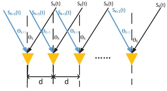
Figure 1.
The system for DOA estimation.
As shown in Figure 1, the phase difference of any two adjacent received signals is:
where is the signal wavelength.
Firstly, consider the situation of one signal, where denotes the n-th received signal at time t.
where is the time interval at which two antennas receive signals.
The received signal can also be written as:
where is the signal frequency.
Thus,
where .
Substituting (4) into (2)
from (1) and (5), we observe that signals received by all antenna arrays are:
Now, considering two unknown signals and , signals received by the n-th antenna element can be expressed as:
Therefore, the signals received in total can be written as:
where , denotes the steering vector for the k-th signal. , , and denotes the additive white Gaussian noise (AWGN).
2.2. System Model with Phase Errors
The unknown phase errors among antennas are not considered in the system model in (9). When we take phase errors into this system model, the received signals are expressed as:
where the matrix of the phase error is defined as a diagonal matrix , , and denotes the phase error of the n-th receiving antenna and .
Finally, with the received signal , the DOA estimation system model with phase errors can be expressed in (9). The direction vector of the signal will be estimated through the method with parameters and signals in the following sections.
3. Sparse-Based Algorithm for DOA Estimation
In this section, a novel direction-finding method based on the Simultaneous Orthogonal Matching Pursuit (SOMP) [42] method is proposed in a scenario with phase errors. SOMP [42] is a multiple measurement vector (MMV) extension of the OMP algorithm. With less strict requirements on the signal sparsity, this method can realize the recovery of sparse signals by increasing the number of measurement vectors. The details about the proposed DOA estimation method with unknown phase errors is given in Algorithm 1.
At Step 4 of Algorithm 1, the estimated sparse matrix is updated by using the SOMP method. The SOMP method for the sparse reconstruction is given in Algorithm 2. The SOMP algorithm is an iterative procedure, and in each iteration of the SOMP method an atom is selected, and the residual is updated. The next was selected to maximize the correlation with the current residual. In this method, we use as the dictionary matrix instead of .
At Step 7 of Algorithm 1, we use a gradient descent method to update the phase errors. A gradient descent is a first-order iterative optimization algorithm applied in finding the minimum of a function. Steps proportional to the negative of the gradient (or approximate gradient) of the function at the current point are taken to find a local minimum of a function using gradient descent. We use the following Lemma to derive the gradient descent method.
| Algorithm 1 The proposed algorithm to estimate the DOAs in the scenario with phase errors among the antennas. |
|
In order to get the steepest descent direction, the derivation is required. The received signal vector can be expressed in another form as:
where .
To get the exact step of every iteration, we define the following objective function:
and the derivation of can be expressed as:
Additionally, the derivation of is:
where is the real part of , and is the image part. Therefore, (12) can be expressed as:
where
and
We adopted as the step for every iteration, where p is a fixed step.
| Algorithm 2 SOMP algorithm to estimate the DOAs |
|
4. Simulation Results
In this section, the simulation results about the proposed method for DOA estimation in the ULA system with unknown phase errors are given, and the simulation parameters are given in Table 1. All experiments were carried out in MATLAB R2018b on a PC with a 2.4 GHz Intel Core i7 and 8 GB of RAM.

Table 1.
Simulation Parameters.
- FISTA: fast iterative shrinkage-thresholding algorithm method proposed in [43]. FISTA provided a new resolution to realize the forward-backward splitting method (also known as the proximal gradient method) splitting to a broad range of problems appearing in sparse recovery, MMV problems, and many other aspects. Whether the problem solved is simple or complex, FISTA simplifies it efficiently by handling issues like stepsize selection, acceleration, and stopping conditions.
- OGSBI: the off-grid sparse Bayesian inference method proposed in [44]. The OGSBI method deals with the off-grid DOA estimation problem and uses an iterative algorithm based on the off-grid model from a Bayesian perspective, while joint sparsity among different snapshots is exploited by assuming a Laplace prior for signals at all snapshots. The OGSBI method applies to both single-snapshot and multi-snapshot cases and has high estimation accuracy, even under a very coarse sampling grid.
- SOMP: for compressed sensing, the critical thing is to extend from the single-measurement vector (SMV) problem to the MMV problem.SOMP, which can recover signals by increasing the number of measurement vectors, is an MMV extension of OMP.
These methods are widely used in DOA estimation, so we made a comparison on the performance of these methods with the proposed method.
The number of antennas, samples, and signals and the value of SNRs are typical simulation parameters. Reference [45] also used these parameters. As a result, we chose these variables as our simulation parameters. After the received signal is generated in the simulation process, phase errors are randomly added to the arrival angels to establish the antenna array model with phase errors. In this paper, we assumed the values of phase errors were from 25° to 35°. These phase errors are described as a uniform distribution between 25° to 35°. The noise given in this paper is the AWGN.
The simulation results of the paper were obtained after multiple Monte Carlo trials. By using the given parameters in the paper, we can reproduce the results.
For different phase errors existed in antennas, where from Figure 2 we can see the corresponding performance of DOA estimation using the proposed method and the SOMP method. The root-mean-square error (RMSE) was used to measure the DOA estimation performance.
where with the i-th experiment, is the vector of a truly received signal, is that with estimation DOA, and is the number of the experiment. In Figure 2, we show the DOA estimation performance with different values of SNR. With the SNR being 20 dB, the DOA estimation performance with different numbers of antennas is given in Figure 2. As shown in this figure, more antennas brings about a better performance of DOA estimation. When the number of antennas reaches 20, the proposed method achieves the best performance. Furthermore, the proposed method achieves a greater improvement compared with the traditional method including SOMP, FISTA, and OGSBI.
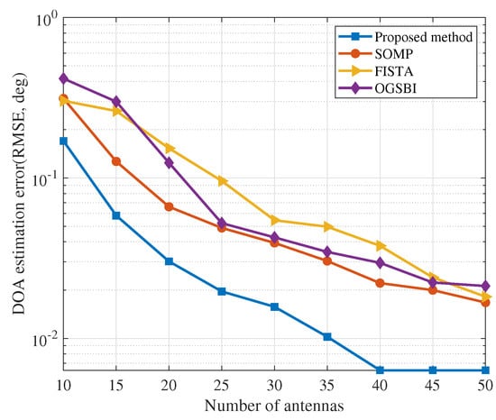
Figure 2.
DOA estimation performance with different numbers of antennas.
We show the DOA estimation performance with different numbers of phase errors in Figure 3. The number of phase errors refers to the number of antennas with large phase errors in the array. Not each antenna is associated with the phase error. In this paper, we assumed 2–4 antennas in ten had large phase errors, and phase errors of other antennas is small. The situation of each antenna that has a large phase error can be converted into the situation with no existent error. With a larger number of phase errors, the performance of the proposed method is better. When there are five phase errors on the antenna system, the proposed method achieves the best performance. The Figure also indicates that existing methods, including SOMP, OGSBI, and FISTA, cannot estimate correctly with an increasing number of phase errors. Therefore, the proposed method is very efficient in the case of large numbers of phase number.
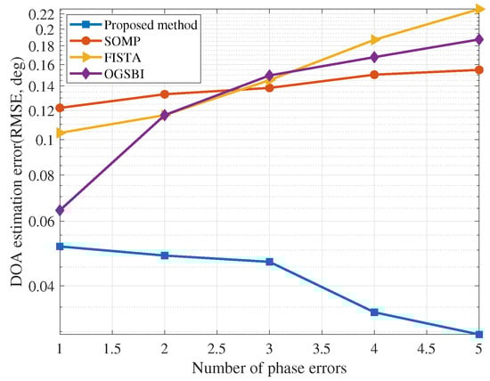
Figure 3.
DOA estimation performance with different numbers of phase errors.
For different sample numbers, Figure 4 shows that further optimization of the sample number can achieve a better resolution. Besides, the Figure shows the proposed method has a much better performance when the sample number changes.
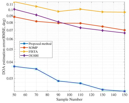
Figure 4.
DOA estimation performance with different numbers of samples.
Additionally, for different SNRs, we can see the DOA estimation performance in Figure 5, where the SNR is from -5 dB to 25 dB. When the SNR is smaller than 15 dB, with the increase of SNR, the DOA estimation performance can be improved. When the SNR is larger than 15 dB, the DOA estimation performance changes slowly with different SNRs. Since the sparse signals and the phase errors are estimated iteratively using the proposed methods, it achieves better performance than the existing methods, including SOMP, FISTA, and OGSBI.
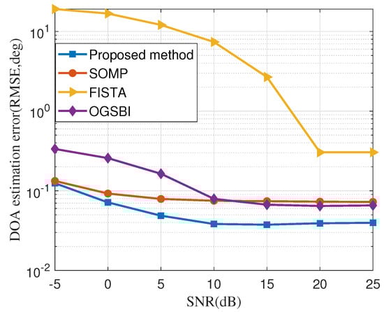
Figure 5.
DOA estimation performance with different SNRs.
We show the DOA estimation performance with different numbers of target signals in Figure 6. As shown in this Figure, a better DOA estimation can be achieved by decreasing the number of target signals using the proposed method. However, when the number is getting larger, the estimation error of the proposed method improves faster compared with the traditional SOMP method. When the number is 6, it achieves the same estimation performance as SOMP, which does not consider the phase errors existing in antennas. Figure 6 indicates that the proposed method has an advantage in that the number of target signals is small, and achieves the best performance among existing methods, including SOMP, FISTA, and OGSBI.
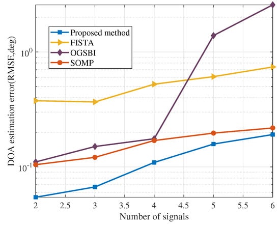
Figure 6.
DOA estimation performance with different numbers of targets.
Finally, the computation time of the proposed method is compared with the present three methods in Table 2. We have not further worked in decreasing the computational time for all the methods. The computational complexities of SOMP in Step 4 and Step 7 are and . Without the additional simplifications, the computational complexities of the proposed method in Step 5 and Step 6 are and . With the conditions and , the computational complexities of the proposed method can be simplified as per iteration. As shown in Table 2, the method SOMP has the least computation time. However, the proposed method has better performance of DOA estimation. The proposed method is comparable with the FISTA method, but the DOA estimation performance is better in the scenario with phase errors among antennas. The computation time of the OGSBI method is much longer than our proposed method. Thus, the DOA estimation performance in the ULA system with phase errors can be significantly improved in the cost of an acceptable computational complexity.
Table 2.
Simulation Time.
5. Conclusions
In this paper, we have investigated the DOA estimation problem of the ULA system in the scenario with unknown phase errors among antennas. The system model considering the additional phase errors was formulated by using a diagonal matrix. The DOA estimation problem can be converted into a sparse reconstruction problem to exploit the signal sparsity in the spatial domain based on the CS theory. Then, a novel method was proposed to estimate DOA, which updates the sparse signals and phase errors iteratively. Simulation results confirm that the performance of DOA estimation using the proposed method outperforms the state-of-the-art methods. Future work will focus on the extension of the proposed method in a scenario with moving platforms.
Author Contributions
Conceptualization, L.L. and X.Z.; Data curation, L.L. and X.Z.; Formal analysis, L.L., X.Z. and P.C.; Funding acquisition, P.C.; Methodology, P.C.; Writing–original draft, L.L. and X.Z.; Writing–review and editing, P.C.
Funding
This work was supported in part by the National Natural Science Foundation of China (Grant No. 61801112), the Natural Science Foundation of Jiangsu Province (Grant No. BK20180357), the Open Program of State Key Laboratory of Millimeter Waves (Southeast University, Grant No. Z201804).
Conflicts of Interest
The authors declare no conflict of interest.
References
- Wang, L.; Zhao, L.; Bi, G.; Wan, C.; Zhang, L.; Zhang, H. Novel Wideband DOA Estimation Based on Sparse Bayesian Learning with Dirichlet Process Priors. IEEE Trans. Signal Process. 2016, 64, 275–289. [Google Scholar] [CrossRef]
- Cao, Z.; Chen, P.; Chen, Z.; He, X. Maximum likelihood-based methods for target velocity estimation with distributed MIMO radar. Electronics 2018, 7, 29. [Google Scholar] [CrossRef]
- Chen, P.; Qi, C.; Wu, L.; Wang, X. Waveform design for Kalman filter-based target scattering coefficient estimation in adaptive radar system. IEEE Trans. Veh. Technol. 2018, 67, 11805–11817. [Google Scholar] [CrossRef]
- Krim, H.; Viberg, M. Two decades of array signal processing research: the parametric approach. IEEE Signal Process. Mag. 1996, 13, 67–94. [Google Scholar] [CrossRef]
- BURG, J.P. Maximum entropy spectral analysis. In Proceedings of the 37th Annual International Meeting, Oklahoma City, OK, USA, 31 October 1967. [Google Scholar]
- Capon, J. High-resolution frequency-wavenumber spectrum analysis. Proc. IEEE 1969, 57, 1408–1418. [Google Scholar] [CrossRef]
- Schmidt, R.O. Multiple emitter location and signal parameter estimation. IEEE Trans. Antennas Propag. 1986, 34, 276–280. [Google Scholar] [CrossRef]
- Chen, J.; Huo, X. Theoretical Results on Sparse Representations of Multiple-Measurement Vectors. IEEE Trans. Signal Process. 2006, 54, 4634–4643. [Google Scholar] [CrossRef]
- Ren, Q.S.; Willis, A.J. Fast ROOT-MUSIC algorithm. Electron. Lett. 1997, 33, 450–451. [Google Scholar] [CrossRef]
- Rao, B.D.; Hari, K.V.S. Performance analysis of ROOT-MUSIC. IEEE Transa. Acoust. Speech Signal Process. 1989, 37, 1939–1949. [Google Scholar] [CrossRef]
- Roy, R.H.; Paulraj, A.; Kailath, T. Comparative performance of ESPRIT and MUSIC for direction-of-arrival estimation. In Proceedings of the IEEE International Conference on Acoustics, Speech, and Signal Processing, Dallas, TX, USA, 6–9 April 1987; Volume 12, pp. 2344–2347. [Google Scholar]
- Roy, R.H.; Kailath, T. ESPRIT-estimation of signal parameters via rotational invariance techniques. Opt. Eng. 1990, 29, 369–411. [Google Scholar]
- Roy, R.H.; Paulraj, A.; Kailath, T. ESPRIT—A subspace rotation approach to estimation of parameters of cisoids in noise. IEEE Trans. Acoust. Speech Signal Process. 1986, 34, 1340–1342. [Google Scholar] [CrossRef]
- Stoica, P.; Arye, N. MUSIC, maximum likelihood, and Cramer-Rao bound. IEEE Transa. Acoust. Speech Signal Process. 1989, 37, 720–741. [Google Scholar] [CrossRef]
- Ottersten, B.; Viberg, M.; Stoica, P.; Nehorai, A. Exact and Large Sample Maximum Likelihood Techniques for Parameter Estimation and Detection in Array Processing; Springer: Berlin/Heidelberg, Germany, 1993; pp. 99–151. [Google Scholar]
- Cadzow, J.A. A high resolution direction-of-arrival algorithm for narrow-band coherent and incoherent sources. IEEE Trans. Acoust. Speech Signal Process. 1988, 36, 965–979. [Google Scholar] [CrossRef]
- Clergeot, H.; Tressens, S.; Ouamri, A. Performance of high resolution frequencies estimation methods compared to the cramer-rao bounds. IEEE Trans. Acoust. Speech Signal Process. 1989, 37, 1703–1720. [Google Scholar] [CrossRef]
- Ziskind, I.; Wax, M. Maximum likelihood localization of multiple sources by alternating projection. IEEE Trans. Acoust. Speech Signal Process. 1988, 36, 1553–1560. [Google Scholar] [CrossRef]
- Candes, E.J.; Wakin, M.B. An introduction to compressive sampling. IEEE Signal Process. Mag. 2008, 25, 21–30. [Google Scholar] [CrossRef]
- Donoho, D.L. Compressed sensing. IEEE Trans. Inf. Theor. 2006, 52, 1289–1306. [Google Scholar] [CrossRef]
- Gilbert, A.C.; Indyk, P. Sparse recovery using sparse matrices. Proc. IEEE 2010, 98, 937–947. [Google Scholar] [CrossRef]
- Donoho, D.L.; Elad, M. Optimally sparse representation in general (nonorthogonal) dictionaries via ℓ1 minimization. Proc. Natl. Acad. Sci. USA 2003, 100, 2197–2202. [Google Scholar] [CrossRef]
- Baraniuk, R.G.; Cevher, V.; Duarte, M.F.; Hegde, C. Model-based compressive sensing. IEEE Trans. Inf. Theory 2010, 56, 1982–2001. [Google Scholar] [CrossRef]
- Baraniuk, R.G. Compressive sensing [lecture notes]. IEEE Signal Process. Mag. 2007, 24, 118–121. [Google Scholar] [CrossRef]
- Chen, P.; Qi, C.; Wu, L.; Wang, X. Estimation of Extended Targets Based on Compressed Sensing in Cognitive Radar System. IEEE Trans. Veh. Technol. 2017, 66, 941–951. [Google Scholar] [CrossRef]
- Tipping, M.E. Sparse bayesian learning and the relevance vector machine. J. Mach. Learn. Res. 2001, 1, 211–244. [Google Scholar]
- Chen, P.; Chen, Z.; Zhang, X.; Liu, L. SBL-based direction finding method with imperfect array. Electronics 2018, 7, 426. [Google Scholar] [CrossRef]
- Chen, P.; Cao, Z.; Chen, Z.; Wang, X. Off-Grid DOA estimation using sparse Bayesian learning in MIMO radar with unknown mutual coupling. IEEE Trans. Signal Process. 2019, 67, 208–220. [Google Scholar] [CrossRef]
- Bishop, C.M.; Tipping, M.E. Variational relevance vector machines. In Uncertainty in Artificial Intelligence; Morgan Kaufmann Publishers Inc.: Burlington, MA, USA, 2000; pp. 46–53. [Google Scholar]
- Yardibi, T.; Li, J.; Stoica, P. Nonparametric and sparse signal representations in array processing via iterative adaptive approaches. In Proceedings of the 42nd Asilomar Conference on Signals, Systems and Computers, Pacific Grove, CA, USA, 26–29 October 2008; pp. 278–282. [Google Scholar]
- Li, J.; Zhu, X.; Stoica, P.; Rangaswamy, M. Iterative Space-Time Adaptive Processing. In Proceedings of the IEEE 13th Digital Signal Processing Workshop and 5th IEEE Signal Processing Education, Marco Island, FL, USA, 4–7 January 2009; pp. 440–445. [Google Scholar]
- Xue, M.; Zhu, X.; Li, J.; Vu, D.; Stoica, P. MIMO radar angle-doppler imaging via iterative space-time adaptive processing. In Proceedings of the IEEE nternational Waveform Diversity and Design Conference, Kissimmee, FL, USA, 8–13 February 2009; pp. 129–133. [Google Scholar]
- Xue, M.; Roberts, W.; Li, J.; Tan, X.; Stoica, P. MIMO radar sparse angle-Doppler imaging for ground moving target indication. In Proceedings of the IEEE Radar Conference, Washington, DC, USA, 10–14 May 2010; pp. 553–558. [Google Scholar]
- Malioutov, D.M.; Cetin, M.; Willsky, A.S. A sparse signal reconstruction perspective for source localization with sensor arrays. IEEE Trans. Signal Process. 2005, 53, 3010–3022. [Google Scholar] [CrossRef]
- Cetin, M.; Malioutov, D.M.; Willsky, A.S. A variational technique for source localization based on a sparse signal reconstruction perspective. In Proceedings of the IEEE International Conference on Acoustics, Speech, and Signal Processing, Orlando, FL, USA, 13–17 May 2002; Volume 3, pp. 2965–2968. [Google Scholar]
- Malioutov, D.M.; Cetin, M.; Willsky, A.S. Source localization by enforcing sparsity through a Laplacian prior: An SVD-based approach. In Proceedings of the IEEE Workshop on Statistical Signal Processing, St. Louis, MO, USA, 28 September–1 October 2003. [Google Scholar]
- Rebolloneira, L.; Lowe, D. Optimized orthogonal matching pursuit Approach. IEEE Signal Process. Lett. 2002, 9, 137–140. [Google Scholar] [CrossRef]
- Ng, B.C.; See, C.M.S. Sensor-array calibration using a maximum-likelihood approach. IEEE Trans. Antennas Propag. 1996, 44, 827–835. [Google Scholar]
- Friedlander, B.; Weiss, A.J. Eigenstructure methods for direction finding with sensor gain and phase uncertainties. Circuits Syst. Signal Process. 1988, 9, 271–300. [Google Scholar]
- Cao, S.; Ye, Z.; Xu, D.; Xu, X. A Hadamard Product Based Method for DOA Estimation and Gain-Phase Error Calibration. IEEE Trans. Aerosp. Electron. Syst. 2013, 49, 1224–1233. [Google Scholar] [CrossRef]
- Liu, A.; Liao, G.; Zeng, C.; Yang, Z.; Xu, Q. An Eigenstructure Method for Estimating DOA and Sensor Gain-Phase Errors. IEEE Trans. Signal Process. 2011, 59, 5944–5956. [Google Scholar] [CrossRef]
- Tropp, J.A.; Gilbert, A.C.; Strauss, M. Algorithms for simultaneous sparse approximation: Part I: Greedy pursuit. Signal Process. 2006, 86, 572–588. [Google Scholar] [CrossRef]
- Goldstein, T.; Studer, C.; Baraniuk, R.G. A field guide to forward-backward splitting with a FASTA implementation. arXiv, 2014; arXiv:1411.3406. [Google Scholar]
- Yang, Z.; Xie, L.; Zhang, C. Off-grid direction of arrival estimation using sparse bayesian inference. IEEE Trans. Signal Process. 2011, 61, 08. [Google Scholar] [CrossRef]
- Chen, P.; Cao, Z.; Chen, Z.; Liu, L.; Feng, M. Compressed sensing-based DOA estimation with unknown mutual coupling effect. Electronics 2018, 7, 424. [Google Scholar] [CrossRef]
© 2019 by the authors. Licensee MDPI, Basel, Switzerland. This article is an open access article distributed under the terms and conditions of the Creative Commons Attribution (CC BY) license (http://creativecommons.org/licenses/by/4.0/).