1. Introduction
A frequency standard is a device that can provide sinusoidal signal with high accuracy and stability, and its frequency value is usually 10 MHz, although in some cases it can be 5 MHz or 1 MHz [
1,
2,
3,
4]. It is undeniable that any specific device that generates standard values is not absolutely stable, and the frequency standard is no exception. Under the influences of internal and external factors, the frequency standard output will change slowly and eventually lead to the failure of its standard reference function [
5,
6,
7,
8,
9,
10]. In this case, it will need to be calibrated. The calibration of frequency standards is performed by high precision frequency standard comparison measurement. A frequency standard comparison measurement is conducted to measure and evaluate the accuracy and stability of frequency standard, which has important practical significance for the rational use of frequency standard in engineering [
11,
12,
13,
14,
15,
16,
17].
Nowadays, commonly used frequency standard comparison methods include oscilloscope method, time interval counting method, beat frequency method, etc. Among these methods, the oscilloscope method is the simplest one. The oscilloscope can graphically display the frequency difference relationship between two sinusoidal signals. When the frequencies of the two standard frequencies in the comparison are strictly equal, a fixed Lissajous-Figure will be displayed on the screen of the oscilloscope. If there is a difference between the two frequencies, the Lissajous-Figure will move relatively on the oscilloscope display screen. The length of time consumed by the period of Lissajous-Figure’s movement will reflect the frequency difference between two frequency standard signals. A stopwatch is usually used to measure the accuracy and stability of the frequency standard indirectly in this measurement method. In order to reduce the human-controlled error of stopwatch, the measuring time can be prolonged appropriately. Many Lissajous-Figure movement cycles can be included in one measurement. Consequently, the human-controlled error can be weakened relatively, and the ultimate measurement error can be reduced. Usually, it takes a long time to realize high precision frequency standard comparison measurement, thus, this method is not suitable for short-term stability measurement of frequency standard. The basic principle of the time interval counting method is that the frequency to be measured and the reference frequency are both shaped into square waves by a voltage comparator, and then, the time difference between them is measured by the time interval counter. The measurement accuracy of this method is determined by the measurement ability of the time interval counter. The internal time scale error and trigger error of the counter itself will directly reflect the measurement error of this method. The beat frequency method is a classical method that can obtain a high measurement resolution by using a common counter. Its core technology is down-conversion, that is to say, mixing the frequency to be measured and the reference frequency to obtain the frequency difference signal (also known as the beat signal) of the frequency to be measured relative to the reference frequency. Because the frequency of the beat signal after mixing is relatively low, the cycle of the beat signal can be counted and measured by common counter. Because the frequency value of the beat signal is much less than the nominal value of the frequency to be measured, compared with the direct measurement of the frequency to be measured, this method can greatly improve the measurement resolution. To be exact, this method can improve the resolution of frequency measurement system by a multiple of beat factor. However, the beat frequency measurement method also has its drawbacks. For example, this method requires that the reference frequency stability be higher than the frequency to be measured. In addition, the internal time scale error and trigger error of the counter used for measurement can also directly reflect the measurement error of this measurement method.
Another frequency standard comparison method that has to be mentioned is the DMTD (Dual Mixing Time Difference) method [
18,
19]. This method combines the advantages of the time interval counting method and the beat frequency method. It down-converts the frequency to be measured and the reference frequency to two low frequency beat signals at the same time. Then, the time difference of the two low frequency beat signals is measured by a time interval counter. The frequency to be measured and the reference frequency in the system have the same nominal value, and there is a frequency deviation between the common oscillator and the frequency to be measured. The measurement resolution of the DMTD system is usually determined by the resolution of the time interval counter and the size of the beat factor. The DMTD method is one of the most accurate methods to realize the comparison measurement between two frequency standards. The implementation of this method requires that the parameters of dual-channel devices should be as similar as possible, so that the common errors of the system can be well offset. Additionally, this method does not require a high stability of the common oscillator, because the error effect of the common oscillator will be mostly offset in the double balanced measurement.
Due to its higher measurement resolution, the DMTD method is adopted by many excellent commercial frequency standard comparison products on sale, such as Timetech’s Phase-comp, Symmetricom’s MMS (Multi-channel Measurement System) and so on. These instruments or systems based on the classical DMTD method have achieved high measurement accuracy. However, they are generally large in size and lack of portability. Even some instruments or systems must use computers with pre-installed high-precision data acquisition cards. High prices are also a common feature of them. Meanwhile, the counter is still used in some DMTD measurement system. The counter itself has some measurement errors, which can directly affect the measurement errors of this method, for example, the ±1 counting error.
This paper focused on the study of frequency standard comparison measurement method based on DMTD, tried to displace the counter and introduce digital signal processing into the classical DMTD method and developed a high precision and miniaturized frequency standard comparator.
2. Frequency Standard Comparator Using Modified DMTD
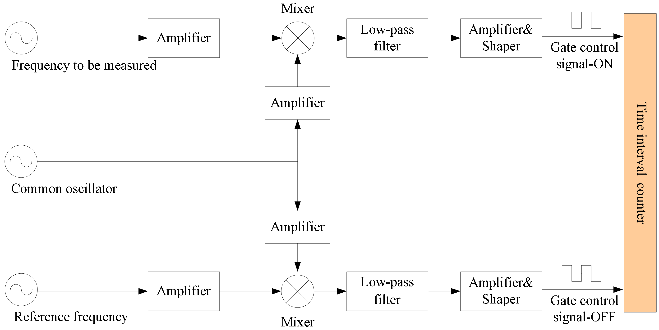
The structural principle of a frequency standard comparator based on traditional DMTD method is shown in
Figure 1. It mixes the frequency to be measured and the reference frequency with the common oscillator respectively at the same time. Then the beat signals were filtered, amplified and reshaped to form two square wave signals. Finally, the time interval counter was used to measure the last phase difference.
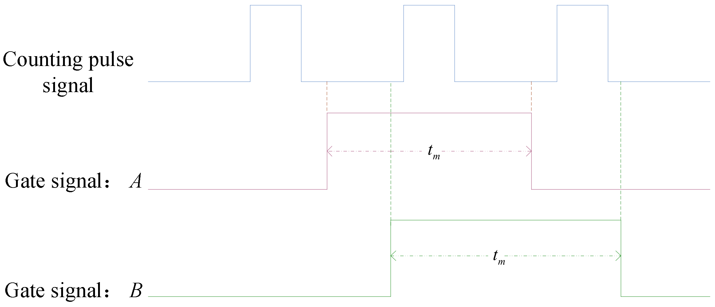
However, the result of the phase difference measurement by a counter is not very accurate. For example, the ±1 counting error is inevitable in the process of phase difference counting measurement. The reason for the ±1 counting error is the uncertainty of the relative displacement between the counting pulse signal and the gate signal of the counter. As shown in the
Figure 2, there are two gate signals with the same length of time
tm,
A and
B. The counting with gate switching
B can get a count of two, and the counting with gate switching
A can get a count of only one.
In this paper, a modified method of the frequency standard comparison measurement based on classical DMTD method was proposed, and a 10 MHz frequency standard comparator was developed. The comparator mainly consisted of a 9.9999 MHz common oscillator, a frequency down-beater that output 100 Hz sinusoidal signals, a dual-channel data simultaneous acquisition module and a digital signal processing module. Unlike the traditional DMTD measurement system, the last unit of the comparator abandoned the counter and replaced it with a digital signal processing module. Two sinusoidal beat signals were sampled at the same time, and then, the phase difference between the frequency to be measured and the reference frequency was calculated by digital signal processing. After down-conversion of the frequency beater, the resolution of phase difference measurement was increased by a multiple of the beat factor. The frequency to be measured and the reference frequency were mixed with the same 9.9999 MHz common oscillator. The symmetrical circuit structure determined that the two sinusoidal beat signals were disturbed by roughly the same noise. The effect of noise from electronic components in two channels on measurement results can be largely offset by subsequent digital correlation processing, thus, it is expected to achieve a good measurement performance.
Just as shown in
Figure 3, the digital signal processing module of the frequency standard comparator was designed based on Field Programmable Gate Array (FPGA). With the development of microprocessors and large scale integrated circuits, digital measurement methods show more advantages, such as higher accuracy, smaller volume, lower cost, better flexibility, etc. [
20,
21,
22,
23,
24,
25]. The realization of signal processing algorithms in digital measurement mostly depends on the platform of computer, MCU (Microcontroller Unit), DSP (Digital Signal Processor) or FPGA (Field Programmable Gate Array). At present, the computer platforms with multi-core processors usually do not have the problem of insufficient computing speed when implementing large data volume algorithms, however, it is difficult to meet the needs of portability and miniaturization of measurement system. The comparatively smaller measurement systems usually use MCU or DSP to implement data processing, where algorithm instructions are usually executed sequentially within their CPU (Central Processing Unit), and the consequent speed bottleneck is inevitable. The application of modern high-speed and large-capacity FPGA is expected to overcome the shortcomings of the above technical solutions. In our design, besides the task of digital signal processing, the FPGA also took into account the functions of controlling data acquisition and output measurement results [
26,
27,
28,
29,
30].
2.1. Common Oscillator
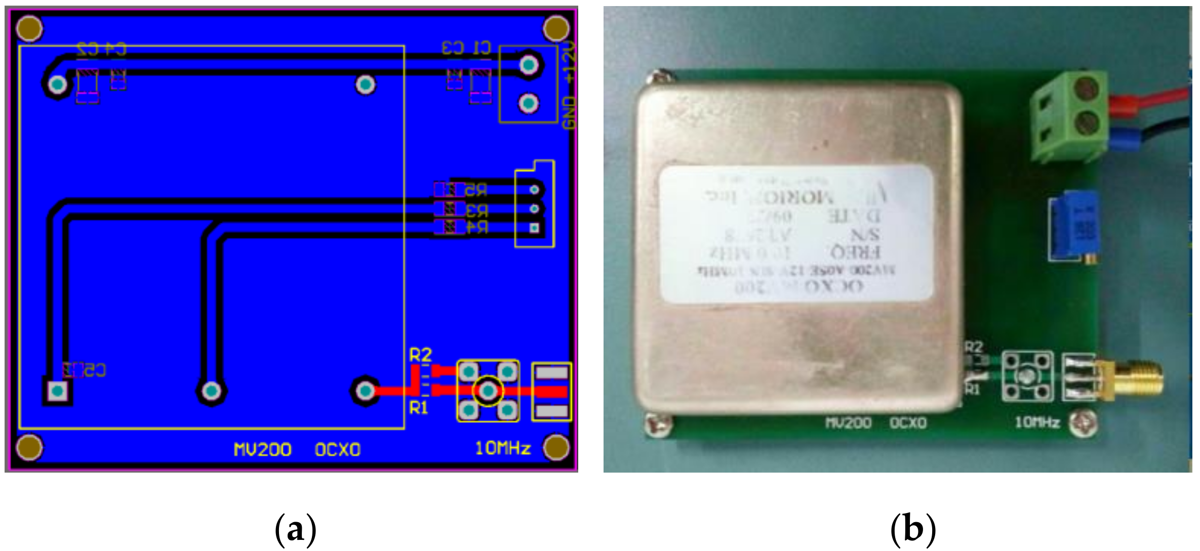
The photograph of the common oscillator is shown in
Figure 4. The core device was an oven controlled crystal oscillator MV200, of which the nominal frequency was 10 MHz. The operating voltage of the common oscillator module is +12 V. Three resistors and one precision potentiometer VR (the blue block devices on the right side of circuit board in
Figure 4b) provided an accurate bias for MV200. By adjusting the potentiometer, the output of the common oscillator SMA-0 (SMA-1 as a backup output, which can be used as a test point) could be stable at 9.999999 MHz.
Figure 4a is the PCB (Printed Circuit Board) photograph of the common oscillator designed in this paper, and
Figure 4b is its physical photograph.
2.2. Frequency Down-Beater
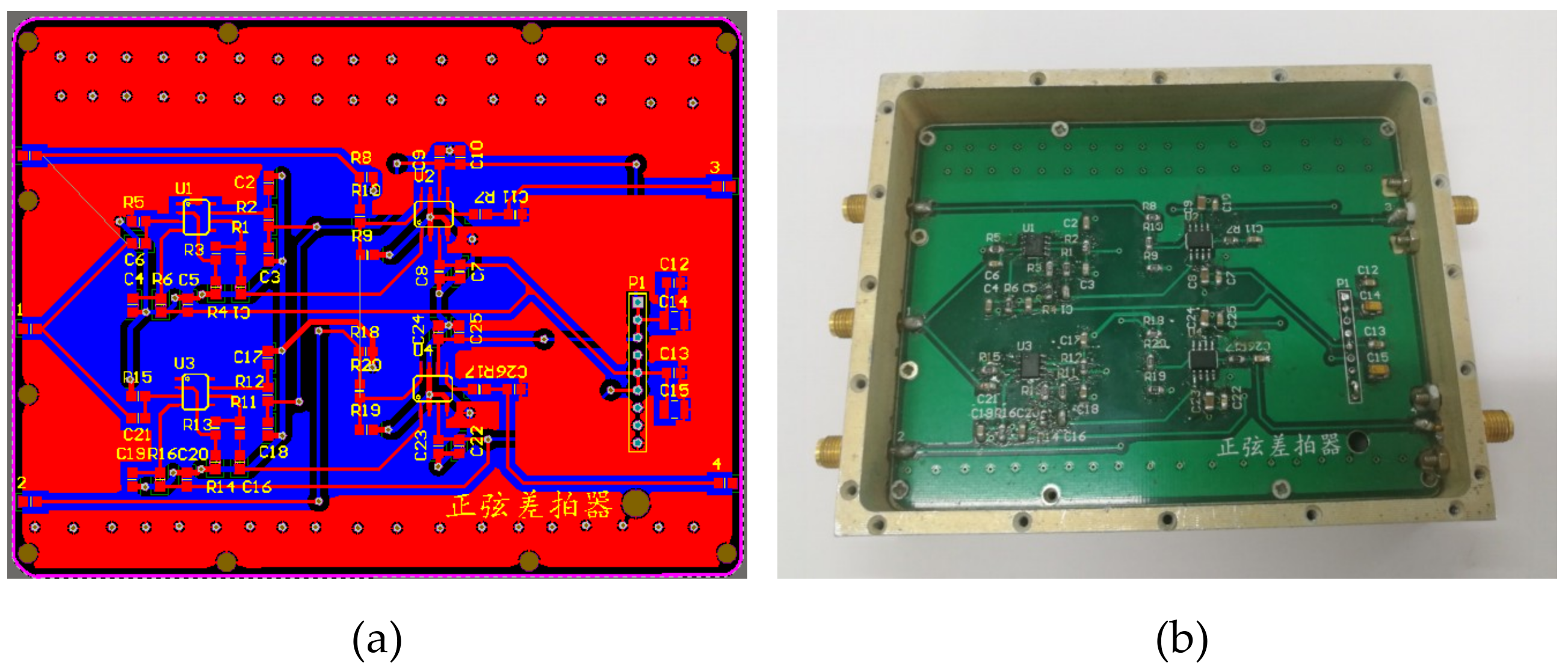
The frequency down-beater mainly consisted of one frequency distribution amplifier and two mixers. Its function was to down-convert the nominal 10 MHz frequencies to 100 Hz low frequency sinusoidal waves. In this paper, two OPA (Operational Amplifier) chips LMH6609 were selected to build an active frequency distribution amplifier with "one in two out", which realized the function of dividing one 9.9999 MHz signal into two without loss and sending them to the mixers, respectively. Additionally, the four quadrant multiplier AD835 was used in the mixers design.
Figure 5a is the PCB photograph of the frequency down-beater designed in this paper, and
Figure 5b is its physical photograph.
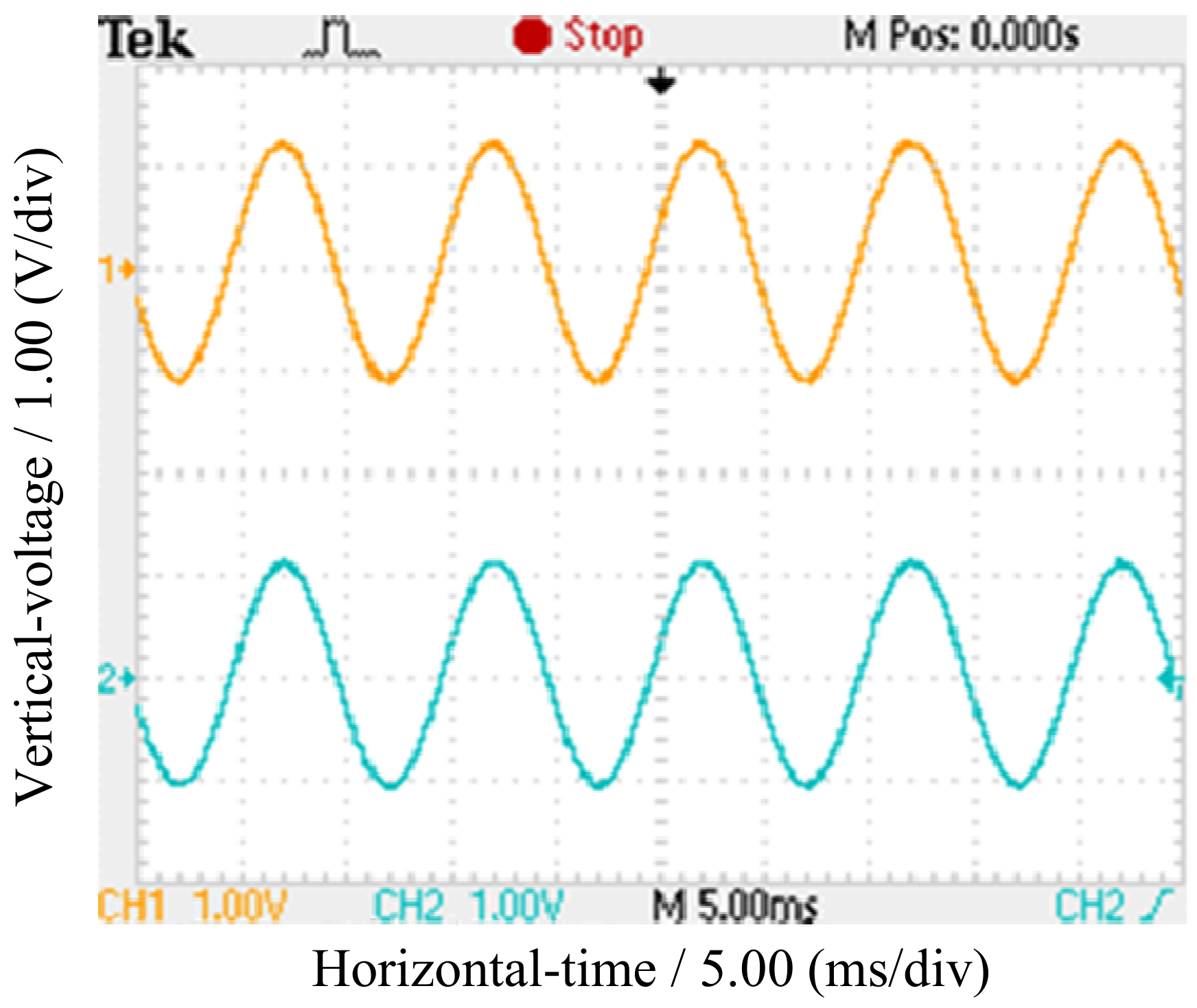
When the output of the common oscillator is 9.9999 MHz and 2.88 Vpp, and the signals to be measured and the reference signal are10 MHz and 3.20 Vpp, the actual outputs of the frequency down-beater were as shown in
Figure 6. The frequency of the two sinusoidal beat signals was 100 Hz, and the peak to peak voltage was about 2.30 Vpp.
2.3. Circuit Module of Signal Sampling, Processing and Transmission
The dual-channel signal sampling circuit proposed in this paper was implemented based on ADS8364 (Texas Instruments Incorporated, Dallas, USA). The non-simultaneous sampling error of ADS8364 was mainly determined by the aperture jitter of the device itself. Aperture jitter was the sampling signal phase error caused by the delay uncertainty of sampling and holding switch in AD converter. Referring to the official data sheet, the typical value of the aperture jitter of ADS8364 was 50 ps. That is to say, the phase error caused by the aperture jitter of ADS8364 was about 1.8 × 10⁻⁶ degrees, which can be neglected in the digital measurement of the phase difference between 100 Hz DMTD beat signals.
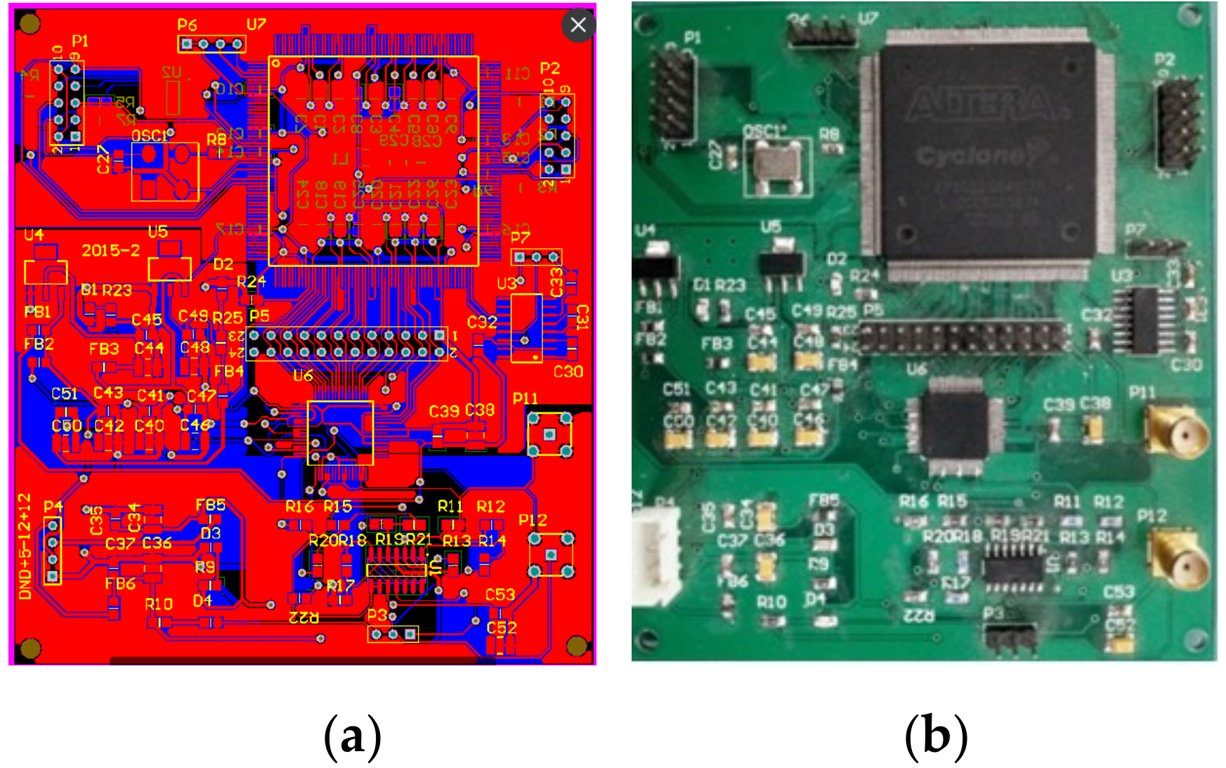
In our design, the digital signal processing module was based on the Hurricane Series FPGA (EP1C12Q240, Altera Company, San Jose, CA, USA). Additionally, the frequency standard comparator used asynchronous serial communication to output the measurement results. The integrated layout of dual-channel data simultaneous sampling circuit, FPGA circuit and serial communication circuit is shown in
Figure 7a, and the corresponding circuit is shown in
Figure 7b.
3. Phase Difference Measurement by Correlation Method Based on FPGA
The phase difference measurement method based on correlation operation was a digital phase difference measurement method, which is widely used in telecommunication, geological exploration, power distribution, aerospace and many other fields. Suppose there are two sinusoidal signals:
where
A and
B represent the amplitudes of the two sinusoidal signals
x(t) and
y(t), respectively,
Nx(t) and
Ny(t) are the noise signals superimposed on
x(t) and
y(t), respectively, and △
φ is the phase difference between two sinusoidal signals.
In the time
T (integer multiple of the signal period), the correlation operation on
x(t) and
y(t) is:
Equation (3) shows that the delay amount
τ affects the cross-correlation function value of the signals
x(t) and
y(t). When
τ = 0, the phase difference △
φ between
x(t) and
y(t) is related to the value of the cross-correlation function
Rxy(0). Since there is usually no correlation between noise and noise, and there is usually no correlation between signal and noise too, if
τ = 0, Equation (3) can be simplified as:
Then, the phase difference between
x(t) and
y(t):
where,
k = 0, 1, 2… If two sinusoidal signals have the same nominal frequency value, then
k = 0. Moreover, because the relationships between the two sinusoidal autocorrelation functions and their phases are
and
, then:
It can be seen from Equation (6) that the phase difference between two sinusoidal signals can be solved by calculating their autocorrelation values and cross-correlation values from the sampled values of them.
In recent years, many scholars have done research on the theory of phase difference measurement based on digital correlation method, and proposed various improved algorithms. In this paper, the phase difference measurement method based on correlation operation was also improved to make it suitable for FPGA implementation. Although FPGA has the advantages of high-speed parallel processing compared with MCU and DSP, it is undeniable that it is less flexible in numerical calculations, especially for arithmetic processing with signed numbers. In order to make our calculation method universally applicable, that is to say, the algorithm could be easily programmed and implemented in both high and low versions of Verilog language, in the system design, the sampling data of the two sinusoidal signals to be measured were simultaneously shifted up by half a peak-to-peak value
a, thereby changing the operation of measuring the phase difference of the entire correlation method into an unsigned operation. Therefore, the two sinusoidal signals to be measured (corresponding to the two 100 Hz signals output by the sinusoidal frequency beater) become:
The autocorrelation coefficients of the above two signals can be calculated as:
Correspondingly, the relationship between the amplitudes of the two new sinusoidal beat signals and their autocorrelation coefficients are:
The correlation coefficients between two signals can be derived:
Then, the phase difference between
x(t) and
y(t) is:
Substituting the Equation (14) into (13), the second expression of the phase difference formula can be obtained, just as shown as:
It can be known from Equations (13) and (15) that the core task of measuring phase difference based on the FPGA correlation method is to implement inverse trigonometric function converter based on Verilog hardware description language. In this paper, Chebyshev polynomial was used to approximate the arctangent function shown in Equation (15), and the calculation of the function was reduced to the form of accumulating polynomial with coefficients, which is implemented in FPGA by iterative algorithm.
Chebyshev polynomial
is an orthogonal polynomial group with a weight function on [-1,1], which can be expressed as:
The recursive formula of Chebyshev is:
The expression that approximates the function to be implemented using the Chebyshev polynomial is:
where the Chebyshev coefficient is:
Since the domain of the Chebyshev function is [-1, 1], the calculation formula outside this range is calculated as:
It can be seen from Chebyshev’s recursive Equation (17) that as the number of iterations increases, it will cause too many multiplications and addition, which leads to the algorithm being too complicated. According to the Chebyshev recursion Equation (17), the function can be implemented in a recursive manner, thereby avoiding the problem that the hardware is difficult to implement as the approximation precision increases. The specific operation process can be described as:
where
is the number of Chebyshev estimation coefficients,
di is the iterative estimation process value, and
f(x) is the estimation result.
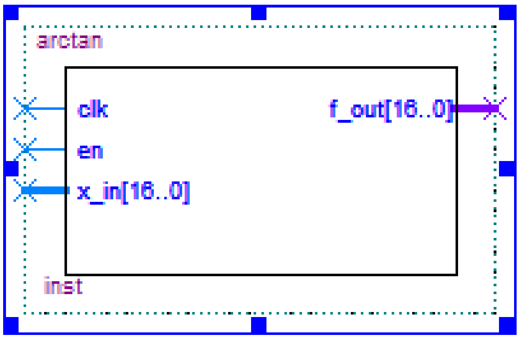
The circuit structure of Chebyshev-based arctangent algorithm generated by Quartus II compilation is shown in
Figure 8. Where ‘clk’ is the clock signal of Chebyshev-based arctangent algorithm. ‘x_in [16..0]’ corresponds to the
x in Equation (22) and ‘fout [16..0]’ is the radians accumulator, corresponding to the
f(x) in Equation (22).
It can be seen from the recurrence process described in Equation (22) that the number of estimation coefficient
M is the main factor affecting the accuracy of phase difference estimation. Additionally, in order to evaluate the accuracy of Chebyshev estimation mentioned above, we designed the following experiment. Two 100 Hz sinusoidal signals (with a presupposed phase difference, e.g. 5) were generated by the function signal generator SDG5162. After data acquisition and processing by the circuit board shown in
Figure 7, the accuracy of phase difference calculation by Chebyshev estimation method can be observed with the on-line debugging tool SignalTap II.
Figure 9 shows the effect of the number of estimation coefficients
M on the phase difference estimation accuracy. As can be seen from
Figure 9, with the increase of the number of estimation coefficient, the accuracy of phase difference estimation gradually improved, and the relative error of phase difference estimation was close to 0.005 when
M = 5. However, this improvement becomes insignificant when the coefficient is greater than 6. In our design, the number of estimation coefficient was set to 6 on a trade-off between estimation accuracy and logical resource consumption of system.
4. Experimental Evaluation
After single board debugging and hardware joint debugging of the common oscillator, sinusoidal frequency beater, dual-channel data simultaneous sampling circuit, FPGA digital signal processing circuit and serial communication circuit, it was necessary to test the whole machine of the frequency standard comparator to determine its indicators, such as relative channel delay, noise floor, etc. In order to obtain more credible experimental results, all of the experimental instruments and equipment were preheated six hours before each measurement.
4.1. Relative Channel Delay
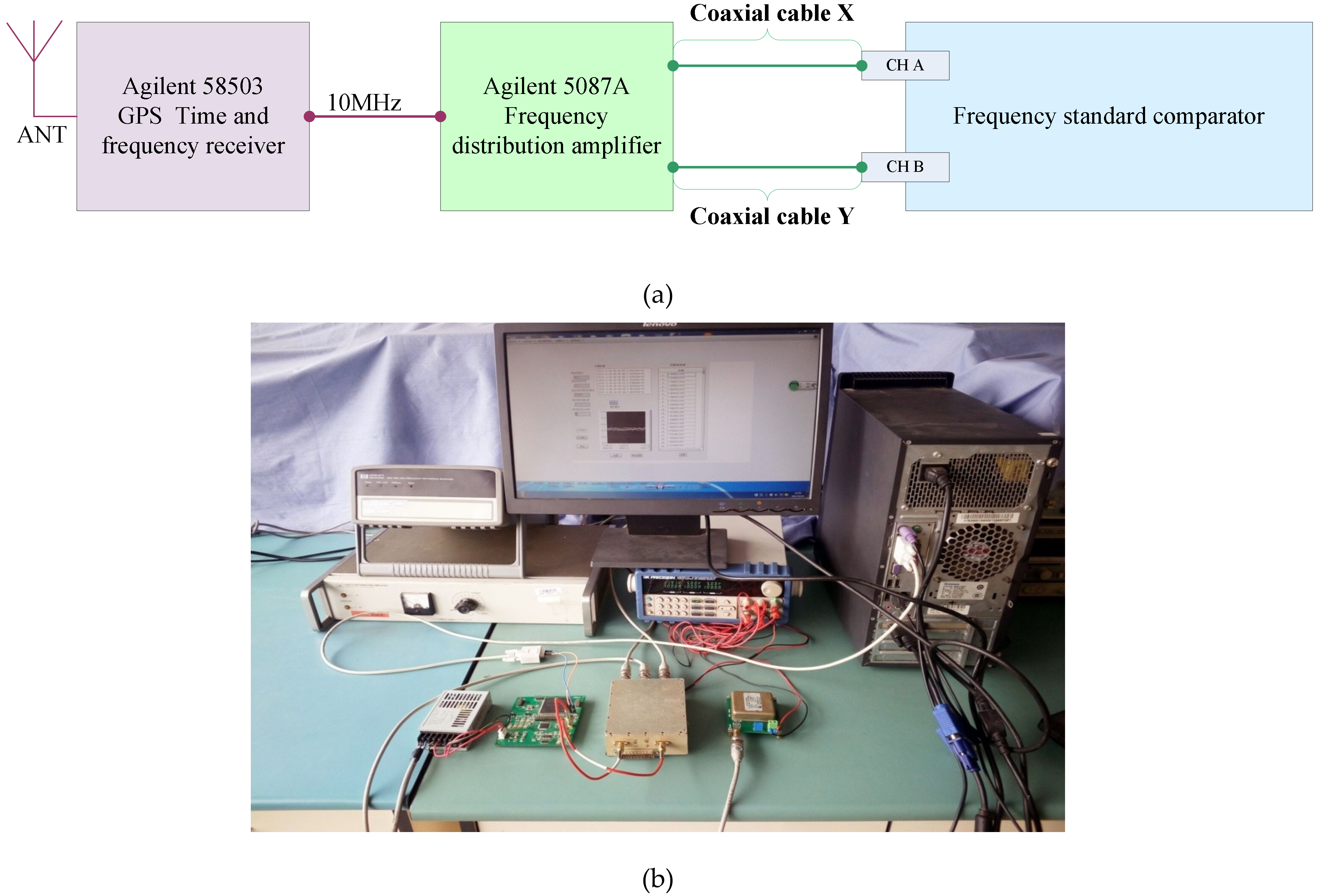
In order to measure the delay difference between the two channels of the comparator, an experimental platform was built as shown in
Figure 10. First of all, the 10 MHz sine wave signal output by the Agilent 58503 GPS (Santa Rosa, CA, USA) time-frequency reference receiver was divided into two identical signals by a frequency distribution amplifier Agilent 5087A (Santa Rosa, CA, USA). Subsequently, they were sent to the comparator’s input channel (CH A) and reference frequency channel(CH B).
In
Figure 10a, the phase differences of the two 10 MHz sinusoidal signals output by the frequency distribution amplifier Agilent 5087A relative to the 10 MHz output signal of the Agilent 58503 were defined as
Tin1 and
Tin2, respectively. Moreover, the time delays caused by the CHA and CHB channels of the frequency standard comparator to the two 10 MHz signals output by the Agilent 5087A were defined as
TCHA and
TCHB. The relative channel delay between CHA and CHB measured by the comparator at this time can be expressed as:
Disconnect the comparator from the coaxial cable X and Y, and the other devices remain the same. Next, the coaxial cable X was connected to the CHB of the comparator, and correspondingly, Y was connected to the CHA. The relative channel delay between CHA and CHB measured by the comparator at this time can be expressed as:
The channel delay of the frequency standard comparator can be obtained by Equations (23) and (24), which can be expressed as:
According to the above method, the relative channel delay of the comparator developed in this paper was 199.60 ps, which is an averaged value of 10 measurements. In order to ensure the authenticity of the measurement results, this delay difference of the channels should be deducted when the FPGA solves the phase difference of the frequency to be measured and the reference frequency.
4.2. Noise Floor
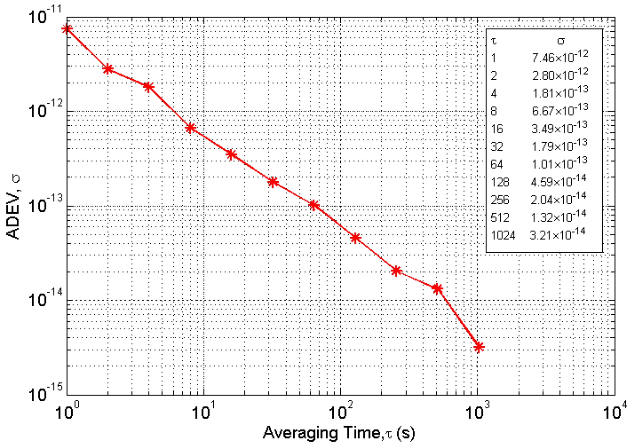
The noise floor is usually used to represent the measurement capability of the frequency standard comparator, which is typically characterized by ADEV (Allan Deviation). The experimental platform used to test the noise floor performance of the comparator is also shown in
Figure 10. The Allan deviation stability of the comparator noise floor that we achieved was less than 7.50 × 10
−12/s, which was obtained by statistics of more than 10000 phase difference measurements (i.e., a measurement result was obtained every second for three consecutive hours), as shown in
Figure 11.
4.3. Measurement Accuracy
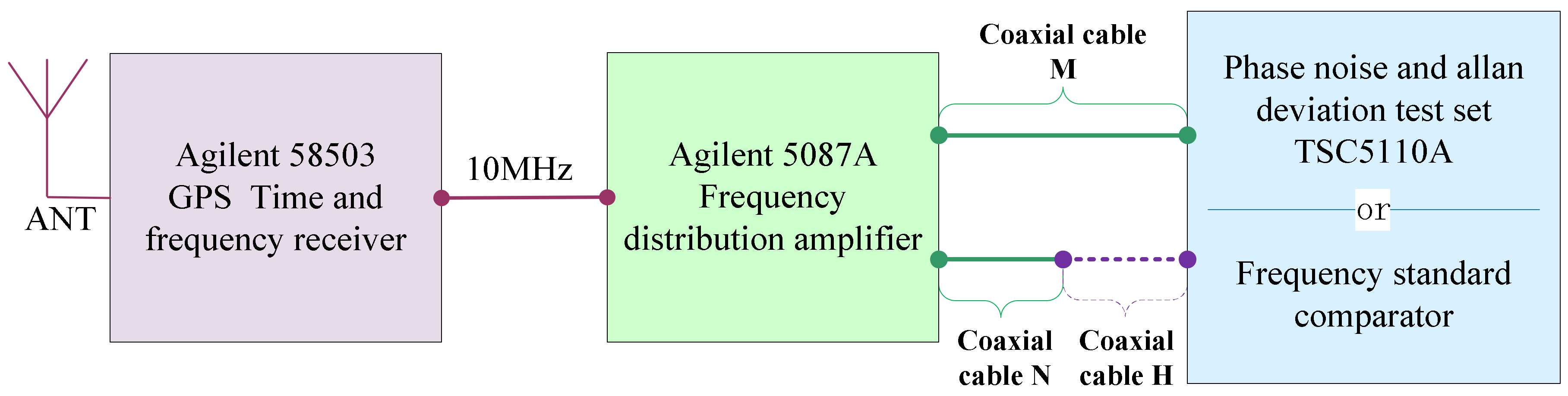
In order to test the phase difference measurement accuracy of the comparator developed in this paper, an experimental platform was built; the structure is shown in
Figure 12. Two sets of experiments were designed.
Experiment 1: The 10 MHz output of Agilent 58503 GPS time-frequency reference receiver was divided into two identical signals by the Agilent 5087A frequency distribution amplifier. Subsequently, they were sent to a phase noise and Allan Deviation test set TSC5110A’s input channel and its reference frequency channel via coaxial cable M and N. Subsequently, a phase difference measurement was carried out, and the measurement result was recorded as △
φ1. In order to add a small amount of phase delay to one of the signals, the coaxial cable H was continued at the rear end of the coaxial cable N. At this time, the two signals of the Agilent 5087A output were input to the TSC5110A by the coaxial cable M and the coaxial cable N+H to perform phase difference measurement, and the result was recorded as △
φ2. Record the amount of phase delay introduced by coaxial cable H as △
φC-5110A. Then, there is:
The measurement results of this experiment were △φ1 = 6.876548 × 10⁻¹⁰ s and △φ2 = 1.261997 × 10⁻⁹ s. Substituting △φ1 and △φ2 into Equation (26), the phase delay of the coaxial cable H for a 10 MHz signal can be calculated, i.e.△φC-5110A = 5.743422 × 10⁻¹⁰ s.
Experiment 2: The above experiment was repeated, however, the phase difference measuring instrument TSC5110(Symmetricom, San Jose, CA, USA) was replaced with the frequency standard comparator proposed in this paper. The two phase difference measurements were defined as △
φ′
1 and △
φ′
2, respectively. Moreover the amount of phase delay introduced by coaxial cable H was recorded as △
φC-FPGA. Then, there was:
The measurement results of this experiment were △φ′1 = 7.394913 × 10⁻¹⁰ s and △φ′2 = 1.313824 × 10⁻⁹ s. Substituting △φ′1 and △φ′2 into Equation (27), the phase delay of the coaxial cable H for a 10 MHz signal can be calculated, i.e. △φC-FPGA = 5.743327 × 10⁻¹⁰ s.
In view of the excellent measurement accuracy of the TSC5110A, it can be approximated that the △φC-5110A measured by the TSC5110A is the true value of the phase delay of the coaxial cable H for the 10 MHz signal. Then, the relative error of the phase difference measurement of the frequency standard comparator developed in this paper can be considered to be about 1.654066 × 10⁻⁵, which was an averaged value of 10 measurements.
5. Conclusions
This paper designed and produced a 9.9999 MHz common oscillator, 100 Hz frequency down-beater, dual-channel data simultaneous sampling circuit, FPGA circuit and serial communication circuit, and performed functional tests on each of the above circuit modules. Finally, these circuit modules were connected together to form a frequency standard comparator. The characteristic work of this paper can be summarized as follows:
(1) An improvement was made to the traditional DMTD method, the counter was discarded, and the phase difference was measured by a digital signal processing method.
(2) The classical phase difference measurement method based on correlation operation was improved to make it suitable for FPGA implementation. Furthermore, the logic operation unit such as inverse trigonometric function converter, digital correlator, multiplier and divider was designed on the FPGA using hardware description language.
(3) A miniaturized 10 MHz frequency standard comparator with good noise floor was successfully developed. The size of the prototype circuit board of the system was only about 292.1 cm2. The noise floor of the comparator was typically better than 7.50 × 10⁻¹²/s, and its relative error of phase difference measurement was less than 1.70 × 10⁻⁵.
The related methods and technical schemes proposed in this paper are expected to provide references for miniaturized frequency standard comparator engineering. However, it should be admitted that there is still a gap between the phase difference measurement resolution of our comparator and some excellent frequency standard comparison instruments on the market. For example, the noise floor of the TSC5110 was only 2.50 × 10⁻¹⁴/s. Therefore, our future work will continue to pursue miniaturization design, while at the same time strive to reduce the noise floor of the frequency standard comparator. Several preliminary research plans can be described briefly as follows:
(1) Seeking or designing better anti-tangent solution than Chebyshev algorithm.
(2) Developing a floating-point unit in FPGA implementation in order to achieve higher phase difference measurement accuracy.
(3) Developing a sinusoidal beater with a higher beat factor. Our next goal is to make the frequency down-beater output a 10 Hz sinusoidal wave with a corresponding beat factor of 10−6, which can theoretically improve the current measurement resolution by an order of magnitude.
(4) Improving circuit manufacture and packaging skill. Miniaturization of the frequency standard comparator is still our unremitting pursuit.


