Stochastic Gradient Matching Pursuit Algorithm Based on Sparse Estimation

Abstract

The stochastic gradient matching pursuit algorithm requires the sparsity of the signal as prior information. However, this prior information is unknown in practical applications, which restricts the practical applications of the algorithm to some extent. An improved method was proposed to overcome this problem. First, a pre-evaluation strategy was used to evaluate the sparsity of the signal and the estimated sparsity was used as the initial sparsity. Second, if the number of columns of the candidate atomic matrix was smaller than that of the rows, the least square solution of the signal was calculated, otherwise, the least square solution of the signal was set as zero. Finally, if the current residual was greater than the previous residual, the estimated sparsity was adjusted by the fixed step-size and stage index, otherwise we did not need to adjust the estimated sparsity. The simulation results showed that the proposed method was better than other methods in terms of the aspect of reconstruction percentage in the larger sparsity environment.

1. Introduction

Compressed sensing (CS) [1,2,3] theory has aroused significant concern over the past few years. It asserts that a signal can be conducted using compressive sampling, which has a much lower frequency than that of Nyquist. The signal processing of an electrical circuit includes an analog-to-digital converter (ADC). The ADC receives an analog input signal, samples the analog input signal based on a sampling clock signal and converts the sampled analog input signal into a digital output signal. The compressed sensing method can be used to sample the analog signal with a lower sample rate than the Nyquist sampling rate. CS theory mainly includes three core issues [4]: (1) The signal sparsity representation, which designs the sparsity basis or the over-complete dictionary with the capability of sparse representation; (2) The compressive measurement of the sparse signal or compressive signal for designing the sensing matrix, which satisfies the incoherence of atoms or restricted isometry property (RIP) [5]; and (3) The reconstruction of the sparse signal is to design the efficiency signal recovery algorithm. In terms of the aspects of signal sparse representation and sensing matrix design, there have been several better solutions. However, extending CS theory to practical applications requires a crucial step to implement, which is the design of a signal recovery algorithm. Therefore, the design of a recovery algorithm is still an important topic in the field of CS research.

Currently, several mature signal recovery algorithms have been proposed. Among the existing recovery algorithms, two major approaches are the $l_1$-norm minimization (or convex optimization) and $l_0$-norm minimization (or greedy pursuit) methods. Convex optimization methods approach the signal by changing the non-convex problem into convex ones such as the basis pursuit (BP) [6] algorithm, the gradient projection for sparse reconstruction (GPSR) [7] algorithm, the interior-point method Bergman iteration (BT) [8] and total-variation (TV) [9]. While the convex optimization methods work correctly for all sparse signals and provide theoretical performance guarantees, its high computational complexity may prevent it from encountering practical large-scale recovery problems. The other category is the greedy pursuit algorithm, which iteratively identifies the true support of the original signal and constructs an approximation signal based on a set of chosen supports until the halt iteration stop condition is satisfied. This can more efficiently solve large-scale data recovery problems. An example of an earlier typical greedy algorithm is the matching pursuit (MP) [10] algorithm. The orthogonal matching pursuit (OMP) [11] algorithm was developed based on the MP algorithm to optimize MP by orthogonalizing the atoms of the support set. However, the OMP algorithm selects one of the columns of preliminary atoms to add the candidate atoms set, which will increase the number of iterations, thereby reducing the speed of the OMP algorithm. Subsequently, some researchers have proposed several modified methods and as for the shortcoming where OMP places only one atom (or column) onto the support atom set at each round of iteration, the stage-wise OMP (StOMP) [12] algorithm has been proposed. StOMP can select multiple atoms to add to the support atom set by using the thresholds. Regularization is introduced in OMP and can provide a powerful theoretical guarantee. This recovery algorithm is called the regularized OMP (ROMP) [13] algorithm. The computational complexity of these algorithms is significantly lower than that of the convex optimization methods; however, they require more measurement of values for exact recovery and have poor reconstruction performance in a noisy environment. To date, subspace pursuit (SP) [14] and compressive sampling matching pursuit (CoSaMP) [15,16] algorithms have been proposed by incorporating a backtracking strategy. These algorithms offer strong theoretical guarantees and provide robustness to noise. However, both of these algorithms require the sparsity $K$ as priority information, which may not be available in most practical applications. In order to overcome this weakness, the sparsity adaptive matching pursuit (SAMP) [17] algorithm was proposed for blind signal recovery when the sparsity is unknown. The SAMP algorithm divides the recovery process of the algorithm into several stages with a fixed step-size and without the prior information of the sparsity. In the SAMP algorithm, the step-size is fixed at the initial stage of the SAMP algorithm. Additional iterations are required if the step-size is much smaller than the signal’s sparsity. This will lead to a long reconstruction time. Furthermore, the fixed step-size cannot estimate the real sparsity precisely because this method can only set the estimated sparsity to a multiple integer of the step-size. Although these traditional greedy pursuit algorithms are widely used due to their simple structure, convenient calculation and better reconstruction effect, they still have many drawbacks. These methods do not directly solve the original optimization problem, which will result in the quality of the signal recovery being of poorer quality than the convex optimization method-based $l_1$-norm. In addition, these greedy pursuit algorithms have the disadvantage of a high computing complexity and large storage capacity for large-scale date recovery.

Since calculating the orthogonal projection requires a large number of calculations using traditional greedy algorithms, this will result in a decline in the recovery efficiency of the greedy algorithm. Thomas et al. first proposed a gradient pursuit (GP) [18] algorithm for the sake of overcoming this shortcoming. This algorithm uses the update of the gradient direction to replace the calculation of the orthogonal projection, which reduces the computational complexity of the greedy pursuit algorithms. Their successors include the Newton pursuit (NP) [19] algorithm, the conjugate gradient pursuit (CGP) [20] algorithm, the approximate conjugate gradient pursuit (ACGP) [21] algorithm and the variable metric method-based gradient pursuit (VMMGP) [22] algorithm. These methods reduce the computational complexity and storage space of the traditional greedy algorithm in terms of the large-scale recovery problem but the reconstruction performance still requires improvement. Therefore, based on the GP algorithm, the stage-wise weak gradient pursuit (SwGP) [23] algorithm was proposed to improve the reconstruction efficiency and convergence speed of the GP algorithm via the weak selection strategy. Although the SwGP algorithm makes the fashioning of atom selection more flexible and improves the reconstruction precision, the time taken for atom selection is greatly increased. Recently, motivated by the stochastic gradient descent methods, the stochastic gradient matching pursuit (StoGradMP) [24] algorithm was proposed for the optimization problem with sparsity constraints. The StoGradMP algorithm not only improves the reconstruction efficiency of the greedy recovery algorithm for the large-scale data recovery problem but also reduces the computational complexity of the algorithm. However, the StoGradMP algorithm still requires the sparsity of the signal as a priori information, which restricts the capacity of the algorithm’s availability in practical situations. This study proposed a sparsity pre-evaluation strategy to estimate the sparsity of the signal and utilized the estimated sparsity as the input parameter of the algorithm. This strategy will make the algorithm eliminate the dependence on signal sparsity and decrease the number of iterations of the algorithm. This algorithm then approaches the real sparsity of the signal by adjusting its initial sparsity estimation, thereby realizing the expansion of the support atoms set and the signal reconstruction.

In recent years, a variety of reconstruction algorithms have been proposed, which have further enhanced the application prospect of CS theory in the field of signal processing such as channel estimation and blind source separation. There is no denying that the application research of reconstruction algorithms will even further highlight the importance of such algorithms. In the literature [25], novel subspace-based blind schemes have been proposed and applied to the sparse channel identification problem. Moreover, the adaptive sparse subspace tracking method was proposed to provide efficient real-time implementations. In Reference [26], a novel unmixing method based on the simultaneously sparse and low-rank constrained non-negative Matrix factorization (NMF) was applied to the remote sensing image analysis.

2. Preliminaries and Problem Statement

In CS theory, for $x\in R^{n\times 1}$, here, $n$ is the length of signal $x$. If the number of non-zero entries is $K$ in original signal, then we regard the signal $x$ as the $K$-sparse signal or compressive signal (in noiseless environments). Generally, the signal $x$ can be expressed as follows:

$$x={\displaystyle \sum _{i=1}^n{\beta }_i{\psi }_i}=\mathsf{\Psi }\beta$$

(1)

$${\parallel \beta \parallel }_0=K$$

(2)

where ${\psi }_i(i=1,2,\dots ,n)$ are the basis vectors of the sparse basis matrix ${\mathsf{\Psi }}^{n\times n}$, that is, $\mathsf{\Psi }$ is the matrix constituted by the ${\left\{{\psi }_i\right\}}_{i=1}^n$. $\beta \in R^n$ is a projection coefficient vector and $K\ll n$. ${\parallel .\parallel }_0$ denotes that the number of non-zero entries in the projection coefficient vector $\beta$.

When the sparse representation of the original signal is completed, we need to construct a measurement matrix $\mathsf{\Phi }$ for the compression measurement of the sparse signal $x$ to obtain the observation values $u$, this process can be described as follows:

$$u=\mathsf{\Phi }x$$

(3)

where $\mathsf{\Phi }\in R^{m\times n}$, $u\in R^{m\times 1}$ and $m\ll n$. According to Equation (3), the observation vector nearly contains the whole information of the $n$-dimensional signal $x$. Furthermore, this process is non-adaptive, which will ensure that the crucial information of the original signal is not lost when the dimensional signal is decreased from $n$ to $m$. The $m$ is called the number of observation values in the later description.

When the original signal $x$ itself is not sparse, the original signal measurement process cannot be directly utilized in Equation (3). Thus, we need the compressive measurement on the projection coefficient vector $\beta$ to obtain the measurement value. According to Equations (1) and (3), we can obtain the follow equation:

$$u=\mathsf{\Phi }\mathsf{\Psi }\beta =\mathsf{\Gamma }\beta$$

(4)

where $\mathsf{\Gamma }=\mathsf{\Phi }\mathsf{\Psi }\in R^{m\times n}$ is the sensing matrix. According to Equation (4), we know that the dimensional of the observation vector $u$ is much lower than the dimensional of signal $x$, that is, $m\ll n$. Therefore, Equation (4) is regarded as an under-determined problem and indicates that Equation (4) has an infinite number of solutions. That is to say, it is hard to reconstruct the projection coefficient vector $\beta$ from observation vector $u$.

Whereas, according to the literature [27], we know that the sufficient condition for exact sparse signal recovery is that sensing matrix $\mathsf{\Gamma }$ satisfies the RIP condition. Thus, if the sensing matrix satisfies the RIP condition, the reconstruction on signal $\beta$ is equivalent to the $l_0$-norm optimization problem [28]:

$$\begin{gathered} \underset{\beta \in R^{n\times 1}}{\min }{\parallel \beta \parallel }_0\mathrm{subject}\mathrm{to} \\ u=\mathsf{\Gamma }\beta \end{gathered}$$

(5)

where ${\parallel .\parallel }_0$ represents the number of non-zero entries in projection coefficient $\beta$. Unfortunately, Equation (5) is a NP-hard optimization problem. When the isometry constant ${\delta }_K$ of the sensing matrix $\mathsf{\Gamma }$ is less than or equal to $\sqrt{2}-1$, Equation (5) is equivalent to the $l_1$-norm optimization problem:

$$\begin{gathered} \underset{\beta \in R^{n\times 1}}{\min }{\parallel \beta \parallel }_1\mathrm{subject}\mathrm{to} \\ u=\mathsf{\Gamma }\beta \end{gathered}$$

(6)

where ${\parallel .\parallel }_1$ denotes that the absolute sum of the non-zero entries in projection coefficient $\beta$. Equation (6) is a convex optimization problem. Meanwhile, when the sparse basis is determined, in order to ensure that the sensing matrix $\mathsf{\Gamma }$ also satisfies the RIP condition, the measurement matrix $\mathsf{\Phi }$ must meet certain conditions. However, in Reference [29,30], the researchers found that when the measurement matrix $\mathsf{\Phi }$ was a random matrix with a Gaussian distribution, the sensing matrix $\mathsf{\Gamma }$ could satisfy the RIP condition with a large probability. This will greatly reduce the difficultly of the design of the measurement matrix.

However, in most practical applications and conditions, the original signal ordinarily contains noise signals. In this setting, this sensing process can be represented in the following equation:

$$u=\mathsf{\Gamma }\beta +\epsilon$$

(7)

where $\epsilon \in R^{n\times 1}$ is the noise signal. In this study, for simplicity, we supposed that the signal $x$ itself was $K$-sparse, thus, the original signal $x$ and sensing matrix $\mathsf{\Gamma }$ were equal to the projection coefficient $\beta$ and measurement matrix $\mathsf{\Phi }$, respectively. According to Equation (7), it can be written as $u=\mathsf{\Phi }x+\epsilon$. We minimized the follow equation to reconstruct the original sparse signal $x$:

$$\begin{gathered} \underset{x\in R^{n\times 1}}{\min }\frac{1}{2m}{\parallel u-\mathsf{\Phi }x\parallel }_2^2\mathrm{subject}\mathrm{to} \\ {\parallel x\parallel }_0\le K \end{gathered}$$

(8)

where $u-\mathsf{\Phi }x$ is the residual of the original signal $x$, which is represented as $r_k$. That is, $r_k=u-\mathsf{\Phi }x$. ${\parallel .\parallel }_2$ represents the square of $l_2$-norm of the signal residual vector $r_k$. To analyze Equation (8), we combined Equation (1). In Equation (1), ${\beta }_i$ is the projection coefficient of the sparse signal $x$. This notion is general enough to address many important sparse models such as group sparsity and low rankness (see studies [31,32] for examples). Then, we can express Equation (9) in the form of

$$\begin{gathered} \underset{x}{\min }\underset{F(x)}{\underbrace{\frac{1}{M}{\displaystyle \sum _{i=1}^M{f}_i(x)}}}\mathrm{subject}\mathrm{to} \\ {\parallel x\parallel }_{0,\mathsf{\Psi }}\le K \end{gathered}$$

(9)

where $f_i(x)$ is a smooth function, that is, it is a non-convex function. ${\parallel x\parallel }_{0,\mathsf{\Psi }}$ is defined as the norm that captures the sparsity of signal $x$.

For a sparse signal recovery problem, the sparse basis $\mathsf{\Psi }$ consists of $n$ basic vectors, each of size $n$ in the Euclidean space. This problem can be regarded as a special case of Equation (9) with $f_i(x)={\left(u_i-<{\varphi }_i,x>\right)}^2$ and $M=m$. The observation vector $u$ is decomposed into the non-overlapping block observation vectors $u_{b_i}$ with a size of $b$. ${\mathsf{\Phi }}_{b_i\times n}$ denotes the block-matrix of the measurement matrix of size $b$. According to Equations (8) and (9), the objective function $F(x)$ can be represented as in the following form:

$$F(x)=\frac{1}{M}{{\displaystyle \sum _{i=1}^M\frac{1}{2b}\parallel u_{b_i}-{\mathsf{\Phi }}_{b_i}x\parallel }}_2^2=\frac{1}{M}{\displaystyle \sum _{i=1}^M{f}_i(x)}$$

(10)

where $M=m/b$, which is a positive integer. According to the equation, each smooth function $f_i(x)$ can be represented as $f_i(x)=\frac{1}{2b}{\parallel u_{b_i}-{\mathsf{\Phi }}_{b_i}x\parallel }_2^2$. Obviously, in this case, each sub-function $f_i(x)$ accounts for a collection (or block) of measurements of size $b$, rather than only one observation. Here, the smooth function $F(x)$ is divided into multiple smooth sub-functions $f_i(x)$ and the measurement matrix $\mathsf{\Phi }$ block into multiple block matrix ${\mathsf{\Phi }}_{b_i}$, which will contribute to the computation of the gradient in the stochastic gradient matching pursuit algorithm, thereby improving the reconstruction performance of the algorithm.

3. StoGradMP Algorithm

The CoSaMP algorithm is fast for small-scale signals with a lower dimensional but for large-scale signals with a higher dimensional and noise signal, the reconstruction precise is not very accurate and the robustness of the algorithm itself is poorly. Therefore, in Reference [30], the researchers generalized the idea of the CoSaMP algorithm and proposed the GradMP algorithm for the reconstruction problem of large-scale signals with sparsity constraints and noise signals. Regrettably, the GradMP algorithm needs to calculate the overall gradient of the smooth function $F(x)$, which increases the computational complexity of the GradMP algorithm. After the GradMP algorithm, Needell et al. proposed a stochastic version of the GradMP algorithm called the StoGradMP [24] algorithm. This algorithm only computes the gradient of the sub-function $f_i(x)$ at each round of iterations.

According to the literature [24], the StoGradMP algorithm is described in Algorithm 1, which consists of the following steps at each round of iterations:

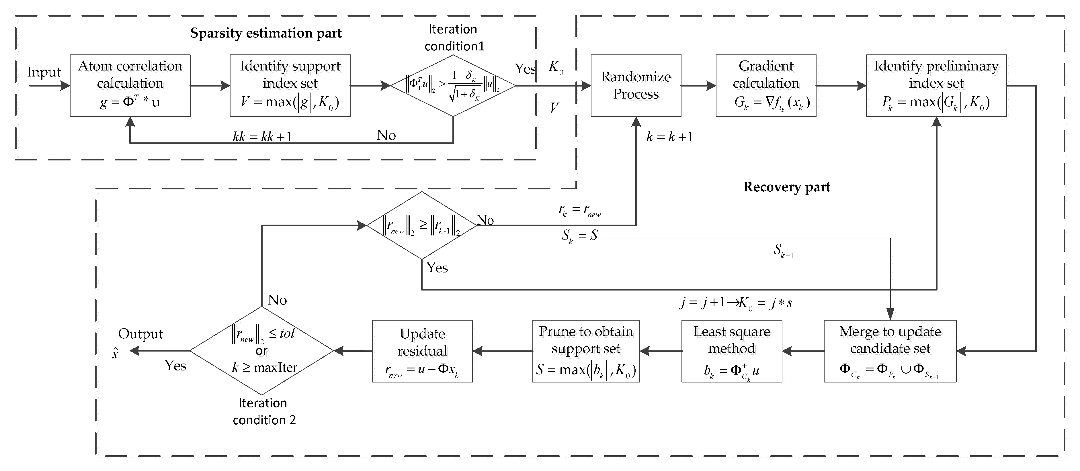
Randomize: The measurement matrix $\mathsf{\Phi }$ is randomly divided into blocks, that is, it searches the row index of the measurement matrix constituting a block matrix ${\mathsf{\Phi }}_{b_i}$ of size $b_i\times n$ by the row vector corresponding to those row indexes. Then, according to Equation (10) and the block matrix, execute the calculation operation of sub-function $f_{i_k}(x_k)$.

Proxy: Compute the gradient $G_k$ of $f_{i_k}(x_k)$, where the gradient $G_k$ is a $n\times 1$ column vector.

Identify: The absolute value of the gradient vector is ranked in descending order, the first $2K$ absolute value of the gradient coefficients are selected, the column index (atomic index) of the measurement matrix corresponding to those coefficients is found, then form a preliminary index set $P_k$.

Merge: Constitute the candidate atomic index set $C_k$, which is consists of the preliminary index set $P_k$ and the support index set $S_{k-1}$ of the previous iteration.

Estimation: The transition estimation of the signal $b_k$ by the least square method.

Prune: The absolute value of the estimation vector of the signal transition is ranked in descending order, the first $K$ absolute value of signal estimation coefficients is determined, then conduct a search for the atomic index of the measurement matrix corresponding to those coefficients, forming the support atomic index set $S_k$.

Update: Update the final estimation of signal $x_k=b_{kS}$ at the current iteration, which corresponds to the support atomic index set $S_k$.

Check: When the $l_2$-norm of the signal residual is less than the tolerance error of the StoGradMP algorithm, the iteration is halted. Or, if the loop index $k$ is greater than the maximum number of iterations, the proposed method ends and the approximation of signal $\widehat{x}=x_k$ is the output. Otherwise, continue the iteration until the halting condition is met.

4. Proposed Algorithm

The StoGradMP algorithm selects $2K$ atoms in each preliminary stage of iteration. Here, $K$ is a fixed number. Therefore, the StoGradMP algorithm requires the sparsity as a priori information, which is not available in practical applications. We first proposed a sparsity pre-evaluation strategy to obtain an estimation of sparsity as a way to overcome this problem. The next step was to put forward a sparsity adjustment strategy to adjust the estimation of sparsity, approaching the real sparsity of the signal.

4.1. Pre-Evaluation Strategy

In this section, we propose a sparsity pre-evaluation strategy to estimate the real sparsity of the original signal. This process is described below.

Firstly, we provided an initial estimation of sparsity, which is $K_0=1$. Next, we calculate the atom correlation $g$, which is expressed as:

$$g={\mathsf{\Phi }}^{T}u$$

(11)

where $\mathsf{\Phi }$, $u$ represents the measurement matrix and observation vector, respectively.

Second, when the calculation of atom correlation is completed, we selected the $K_0$ atoms from the measurement matrix $\mathsf{\Phi }$ to expand the support atom set ${\mathsf{\Phi }}_V$, where the support atomic index can be expressed as:

$$V=\max (|g|,K_0)$$

(12)

where $|g|$ is the absolute value of the atom correlation coefficients $g$. $\max \left(|g|,K_0\right)$ represents finding the atomic (or column) index of matrix $\mathsf{\Phi }$, corresponding to the $K_0$ maximal value from $|g|$.

Finally, we checked the iterative stopping condition of the sparsity evaluation to determine whether to continue to the next iteration and update the iterative parameters. This condition is expressed as:

$${\parallel {\mathsf{\Phi }}_V^{T}u\parallel }_2\ge \frac{1-{\delta }_K}{\sqrt{1+{\delta }_K}}{\parallel u\parallel }_2$$

(13)

where ${\mathsf{\Phi }}_V$ represents the support atomic set (or matrix) corresponding to the support atomic index set $V$. ${\parallel .\parallel }_2$ denotes the $l_2$-norm of a vector. The element ${\delta }_K$ is the isometry constant and ${\delta }_K\in (0,1)$. If the iteration stopping criteria is satisfied, then the output is the estimated sparsity $K_0$ and the support atomic index set $V$, otherwise, the iteration is continued and the estimated sparsity $K_0=K_0+1$ is updated to gradually approach the real sparsity of the original signal until the conditions are satisfied. In addition, the set $V$ will be used for the initial support atomic set estimation in the recovery algorithm. This is $S_0=\mathrm{V}$, which will be used to reduce the selection time of the support atoms set in the recovery algorithm and improve the reconstruction precision.

4.2. Adjustment Strategy

In Section 4.1, we utilized the sparsity pre-evaluation strategy to obtain the sparsity estimation $K_0$ and the support atomic index set $V$. However, the sparsity estimation level was lower than the real sparsity of the original signal. If we used it as an input for the recovery algorithm, it would have resulted in the lack of sparsity estimation, which would have led to a decline in the proposed method in terms of reconstruction performance.

Therefore, we proposed an adjustment strategy for the sparsity estimation to control the convergence conditions of the recovery algorithm and adjust the estimated sparsity $K_0$. This strategy is described below.

We started by checking the iterative stopping condition that is expressed as:

$$\begin{gathered} {\parallel r_{new}\parallel }_2\le tol\mathrm{or} \\ k\ge \mathrm{maxIter} \end{gathered}$$

(14)

where $tol$ is a threshold and $k$ and $\mathrm{maxIter}$ is the number of iterations and the maximum number of iterations, respectively. In addition, $r_{new}$ is the residual at the $k\text{-}\mathrm{th}$ iteration. It can be expressed as:

$$r_{new}=u-\mathsf{\Phi }{x}_k$$

(15)

$$x_k=b_{kS}$$

(16)

where $x_k$ is the approximation of the signal $x$ at the $k\text{-}\mathrm{th}$ iteration. Furthermore, $b_{kS}$ is the estimation vector corresponding to the support atomic index set $S$. The set $S$ is expressed as:

$$S=\max \left(|b_k|,K_0\right)$$

(17)

$$b_k={\mathsf{\Phi }}_{C_k}^{+}u$$

(18)

where $b_k$, $K_0$ is the least solution of the signal and the estimated sparsity at the $k\text{-}\mathrm{th}$ iteration. In addition, $\max \left(|b_k|,K_0\right)$ represents finding the atomic (or column) index of the measurement matrix $\mathsf{\Phi }$ corresponding to the largest $K_0$ value from $|b_k|$ and constitutes the final (or support) atomic set $S$. Furthermore, ${\mathsf{\Phi }}_{C_K}^{+}$ is the pseudo inverse matrix of the candidate atomic set (or matrix) ${\mathsf{\Phi }}_{C_k}$ and its definition is consistent with the definition in the StoGradMP algorithm.

Second, according to Equation (13), we can see that if the iteration stopping condition is not satisfied, we can judge the stage switching condition to complete the goal of adjusting the estimated sparsity. The condition can then be described as:

$${\parallel r_{new}\parallel }_2\ge {\parallel r_{k-1}\parallel }_2$$

(19)

then

$$\begin{gathered} j=j+1\mathrm{and} \\ {K}_0=j\ast s \end{gathered}$$

(20)

where $j$, $s$ are the stage index and the iterative step-size, respectively. Among these, $s$ is a fixed number. In this paper, we set the step-size set as $s=1,5,10,15$, with $K_0$ as the estimated sparsity at the $j\text{-}\mathrm{th}$ stage. If

$${\parallel r_{new}\parallel }_2\le {\parallel r_{k-1}\parallel }_2$$

(21)

then continue to iterate and update the parameters:

$$\begin{gathered} S_k=S\mathrm{and} \\ {r}_k=r_{new} \end{gathered}$$

(22)

where $r_k$ and $S_k$ are the current residual and the support index set at the $k\text{-}\mathrm{th}$ iteration, respectively.

4.3. Reliability Verification Condition

Finally, according to Equation (18), before obtaining the least square solutions of the signal, we needed to add a reliability verification condition to ensure that the proposed method was correct and effective. This condition was that the number of rows was greater than the number of columns in the candidate atomic matrix ${\mathsf{\Phi }}_{C_k}$, that is, ${\mathsf{\Phi }}_{C_k}$ is a full column-rank matrix. This condition can then be described as:

$$length(C_k)\le m$$

(23)

then

$$b_k={\mathsf{\Phi }}_{C_k}^{+}u$$

(24)

where $m$ is the number of the rows in the measurement matrix. The definition of $b_k$, ${\mathsf{\Phi }}_{C_k}^{+}$ and $u$ keep pace with the definition in Equation (18). If the condition is not met, that is to say, the candidate atomic matrix is not inverse, then we set $b_k=0$ and the exit loop.

Figure 1 is a block diagram of the proposed algorithm. As can be seen from Figure 1, the algorithm includes sparsity estimation and restoration. In the sparsity estimation part, the real sparsity estimation is obtained by using the sparsity pre-evaluation strategy. In the recovery part, the sparsity adjustment strategy is proposed to approach the real sparse gradually. This improves the reconstruction accuracy and convergence of the proposed algorithm. The key innovation of the algorithm is that the signal can be recovered without prior sparsity information $K$.

The entire procedure is shown in Algorithm 1.

Algorithm 1 Proposed algorithm
Input:  Measurement matrix ${\mathsf{\Phi }}^{m\times n}$, Observation vector $u$, Block size $b$ Step-size $s$, Isometry constant ${\delta }_K$, Initial sparsity estimation $K_0=1$ Tolerance used to exit loop $tol$, Maximum number of iterations $\mathrm{maxIter}$
Output1:  $K_0$ sparsity estimation of the original signal $V$  the support atomic index set Output2:  $\widehat{x}=x_k$ $K$-sparse approximation of signal $x$
Set parameters:
$\widehat{x}=0$	{initialize signal approximation}
$k=0$	{loop index used to loop 2}
$kk=0$	{loop index used to loop 1}
$done1=0$	{while loop 1 flag}
$done2=0$	{while loop 2 flag}
$r_k=u$	{initialize residual}
$\mathrm{M}=\mathrm{floor}(\mathrm{m}/\mathrm{b})$	{number of blocks}
$P_0=[]$	{empty preliminary index set}
$C_0=[]$	{empty candidate index set}
$V=[]$	{empty support index set used to loop 1}
$S_0=[]$	{empty support index set used to loop 2}
$j=0$	{stage index}
Part 1: Sparsity Estimation While ($~done1$)    $kk=kk+1$ (1) Compute the atom correlation:$g={\mathsf{\Phi }}^T\ast u$ (2) Identify the support index set:$V=\max (|g|,K_0)$ (3) Check the iteration condition   If (${\parallel {\mathsf{\Phi }}_{\mathsf{\Gamma }}^{T}u\parallel }_2>\frac{1-{\delta }_K}{\sqrt{1+{\delta }_K}}{\parallel u\parallel }_2$)     $done1=1$        quit iteration   else     $K_0=K_0+1$    Sparsity approach   end end
Part 2: Recovery part   $S_0=V$   Update the support index set While ($~done2$)   $k=k+1$ (1) Randomize $ii=ceil(rand\ast M)$$\to$$block=b\ast (ii-1)+1:b\ast ii$$\to$$f_{i_k}(x_k)=\frac{1}{2b}{\parallel u_{b_{i_k}}-{\mathsf{\Phi }}_{b_{i_k}}x\parallel }_2^2$ (2) Computation of gradient:$G_k=\nabla f_{i_k}(x_k)=-2\ast {\mathsf{\Phi }}_{b_{i_k}}^T(u_{b_{i_k}}-{\mathsf{\Phi }}_{b_{i_k}}{x}_{k-1})$ (3) Identify the large$K_0$components:$P_k=\max (|G_k|,K_0)$ (4) Merge to update candidate index set:${\mathsf{\Phi }}_{C_k}={\mathsf{\Phi }}_{P_k}\cup {\mathsf{\Phi }}_{S_{k-1}}$   Reliability verification condition       If $length(C_k)\le m$       $b_k={\mathsf{\Phi }}_{C_k}^{+}u$ Signal estimation by the least square method  else          $b_k=0$          break;       end (5) Prune to obtain current support index set:$S=\max (|b_k|,K_0)$ (6) Signal approximation by the support set:$x_k=b_k{}_S$,$r_{new}=u-\mathsf{\Phi }{x}_k$ (7) Check the iteration condition If (${\parallel r_{new}\parallel }_2\le tol$ or $k\ge \mathrm{maxIter}$)   $done2=1$      quit iteration else if (${\parallel r_{new}\parallel }_2\ge {\parallel r_{k-1}\parallel }_2$)  sparsity adjustment condition   $j=j+1$ shift into stage   $K_0=j\ast s$ approach the real sparsity else   $r_k=r_{new}$ update the residual   $S_k=S$ update the support index set end end

5. Proof of the Proposed Algorithm

In this section, we prove the correctness of the pre-evaluation strategy. The main idea of this strategy is to carry out the matching test of atoms to obtain the support atomic index set $V$. The size of the potential of the set $V$ is $K_0$ and $K_0$ is smaller than $K$. Here, $K_0$, $K$ is the estimated sparsity and the real sparsity of the original signal, respectively. The potential of a set is represented by $\mathrm{supp}(.)$. We assumed that the real support of the original signal $x$ could be represented by $F$ and $\mathrm{supp}\left(\mathrm{F}\right)=K$. ${\mathsf{\Phi }}_F$ represents a sub-matrix formed by the atoms (or columns) of the measurement matrix $\mathsf{\Phi }$, whose indices correspond to the real support index set $F$. Moreover, $g={\mathsf{\Phi }}^{T}u$, $g_i$ is the $i\text{-}\mathrm{th}$ element of the atomic correlation coefficient $g$. In addition, the set $V$ consists of indices corresponding to the $K_0$ largest absolute value of $g_i$ and $\mathrm{supp}\left(\mathrm{V}\right)=K_0$. Finally, the proposition can be explained as follows.

Proposition 5.1.

Assume that measurement matrix $\mathsf{\Phi }$ satisfies the restricted isometry property with parameters $K$ and ${\delta }_K$. If $K_0\ge K$, then we can obtain the formula in the form:

$${\parallel {\mathsf{\Phi }}_V^{T}u\parallel }_2\ge \frac{1-{\delta }_K}{\sqrt{1+{\delta }_K}}{\parallel u\parallel }_2$$

(25)

Proof. 

Select the atomic index of matrix $\mathsf{\Phi }$ corresponding to the $K$ largest value from $|g|$ and form the real support atomic index set $F$. When $K_0\ge K$, $F\subseteq V$. Then, we can obtain

$${\parallel {\mathsf{\Phi }}_V^{T}u\parallel }_2\ge \parallel {\mathsf{\Phi }}_F^{T}u\parallel$$

(26)

Furthermore, we have

$$\begin{array}{cc}\hfill {\parallel {\mathsf{\Phi }}_V^{T}u\parallel }_2& =\underset{|F|=K}{\max }\sqrt{{\displaystyle \sum _{i\in F}{|\langle {\mathsf{\Phi }}_i,u\rangle |}^2}}\hfill \\ & \ge {\parallel {\mathsf{\Phi }}_F^{T}u\parallel }_2={\parallel {\mathsf{\Phi }}_F^T{\mathsf{\Phi }}_{F}x\parallel }_2\hfill \end{array}$$

(27)

According to the definition of RIP, the range of the singular value of ${\mathsf{\Phi }}_F$ is $\sqrt{1-{\delta }_K}\le \sigma \left({\mathsf{\Phi }}_F\right)\le \sqrt{1+{\delta }_K}$. Here, $\sigma (.)$ represents a singular value of the matrix. If we denote $\lambda \left({\mathsf{\Phi }}_F^T{\mathsf{\Phi }}_F\right)$ as the eigenvalue of matrix ${\mathsf{\Phi }}_F^T{\mathsf{\Phi }}_F$, we have $1-{\delta }_K\le \lambda \left({\mathsf{\Phi }}_F^T{\mathsf{\Phi }}_F\right)\le 1+{\delta }_K$. Therefore, we can obtain a formula in the form:

$${\parallel {\mathsf{\Phi }}_F^T{\mathsf{\Phi }}_{F}x\parallel }_2\ge \left(1-{\delta }_K\right){\parallel x\parallel }_2$$

(28)

On the other hand, according to the definition of RIP properties, we can obtain the following formula:

$${\parallel x\parallel }_2\ge \frac{{\parallel u\parallel }_2}{\sqrt{1+{\delta }_K}}$$

(29)

Combining the inequalities of Equations (27)–(29), the following formula can be obtained:

$${\parallel {\mathsf{\Phi }}_V^{T}u\parallel }_2\ge \frac{1-{\delta }_K}{\sqrt{1+{\delta }_K}}{\parallel u\parallel }_2$$

(30)

Therefore, the proof is completed. □

In light of the relationship between Proposition 5.1 and its converse-negative propositions, that is to say, if Proposition 1 is true, then its converse-negative proposition is also true. Therefore, for Proposition 1 in this paper, we have

$${\parallel {\mathsf{\Phi }}_V^{T}u\parallel }_2<\frac{1-{\delta }_K}{\sqrt{1+{\delta }_K}}{\parallel u\parallel }_2$$

(31)

Then $K_0<K$.

According to Proposition 1, we can obtain an estimation method of true sparsity $K$. That is, if we obtain an index set $V$ satisfying the inequality (Equation (31)), then the sparsity estimation $K_0$ can be obtained. We can describe this as follows: first, we set the initial estimated sparsity as $K_0=1$ and if the inequality (Equation (31)) is true, then $K_0=K_0+1$. Exit the loop when inequality (Equation (31) is false. Meanwhile, we can obtain an initial index set $V$, which is the estimation of the true support index set $F$.

6. Discussion

In this section, we used the signal with different $K$-sparsity as the original signal. The measurement matrix was randomly generated with a Gaussian distribution. All performances were an average calculated after running the simulation 100 times using a computer with a 32-core, 64-bit processor, two processors and a 32 G memory. We also set the recovery error of all recovery methods as $1\times e^{-6}$ and the tolerance error as $1\times e^{-7}$. The maximum number of iterations of the recovery part of the proposed method was $500\ast M$.

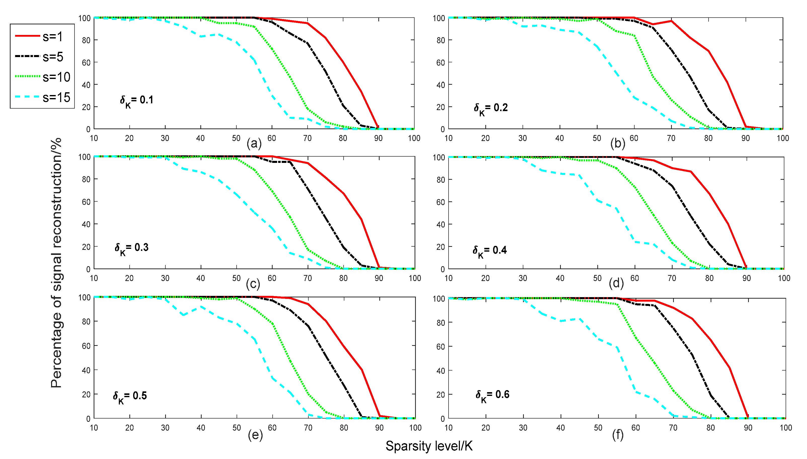
In Figure 2, we compared the reconstruction percentage of different step-sizes of the proposed method with different sparsities in different isometry constants. We set the step size set and the range of sparsity as $s\in [1,5,10,15]$ and $K\in [10100]$, respectively. The isometry constant parameter set was ${\delta }_K\in [0.1,0.2,0.3,0.4,0.5,0.6]$. From Figure 2, we can see that the reconstruction percentage was very close, with almost no difference for all isometry constants ${\delta }_K$. This means that the selection of the isometry constants had almost no effect on the reconstruction percentage of the signal.

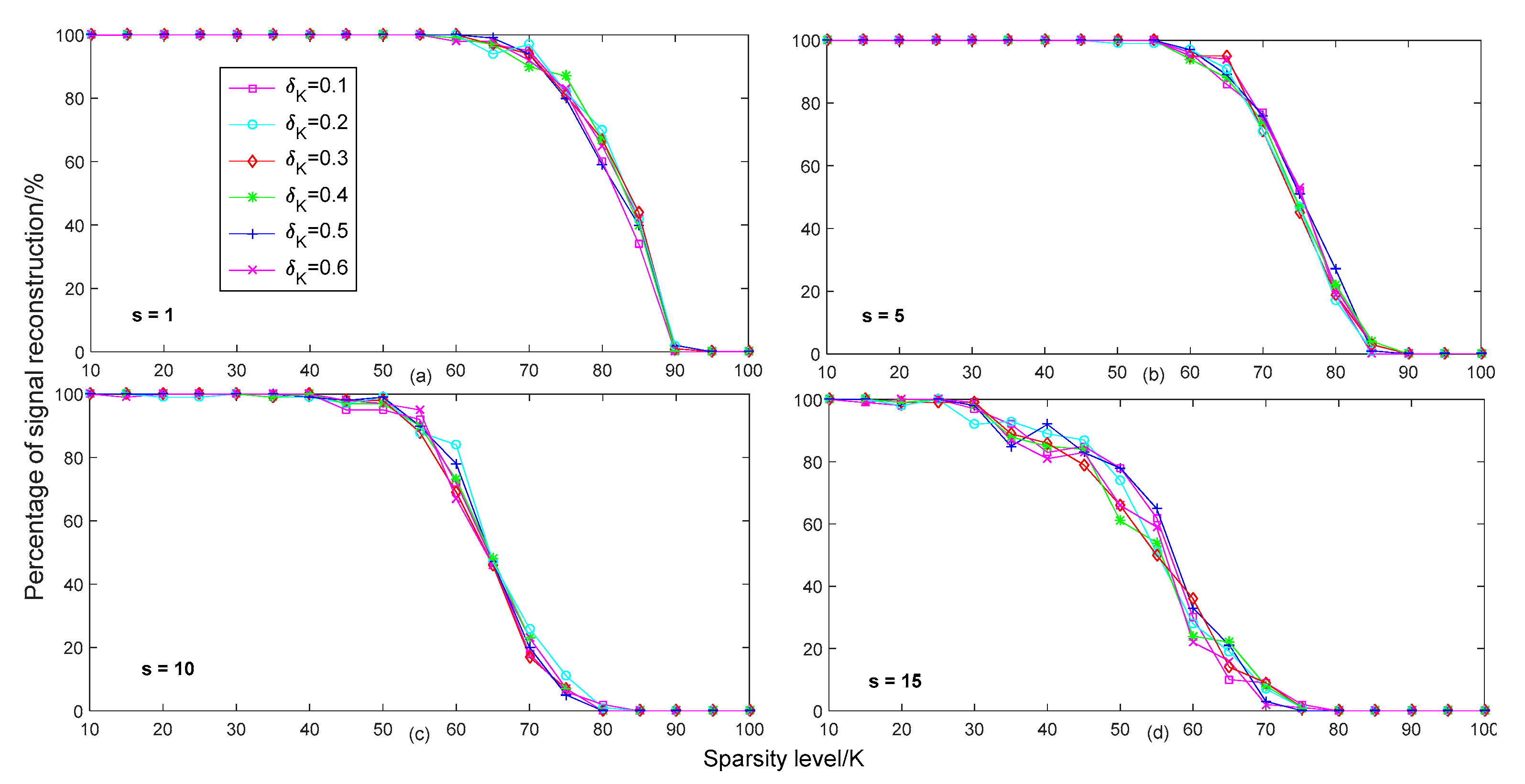
In Figure 3, we compared the reconstruction percentage of different isometry constants ${\delta }_K$ with different sparsities in different step-size conditions. In order to better analyze the effects of different step-sizes on the reconstruction percentage, the setting of parameters in Figure 3 was consistent with the parameters in Figure 2. From Figure 3, we can see that when the step-size $s$ was 1, the reconstruction performance was the best for different isometry constants. When the step size continued to increase, the reconstruction percentage of the proposed method gradually declined. In particular, when the step-size $s$ was 15, the reconstruction performance was the worst. This shows that a smaller step-size benefits the reconstruction of the signal.

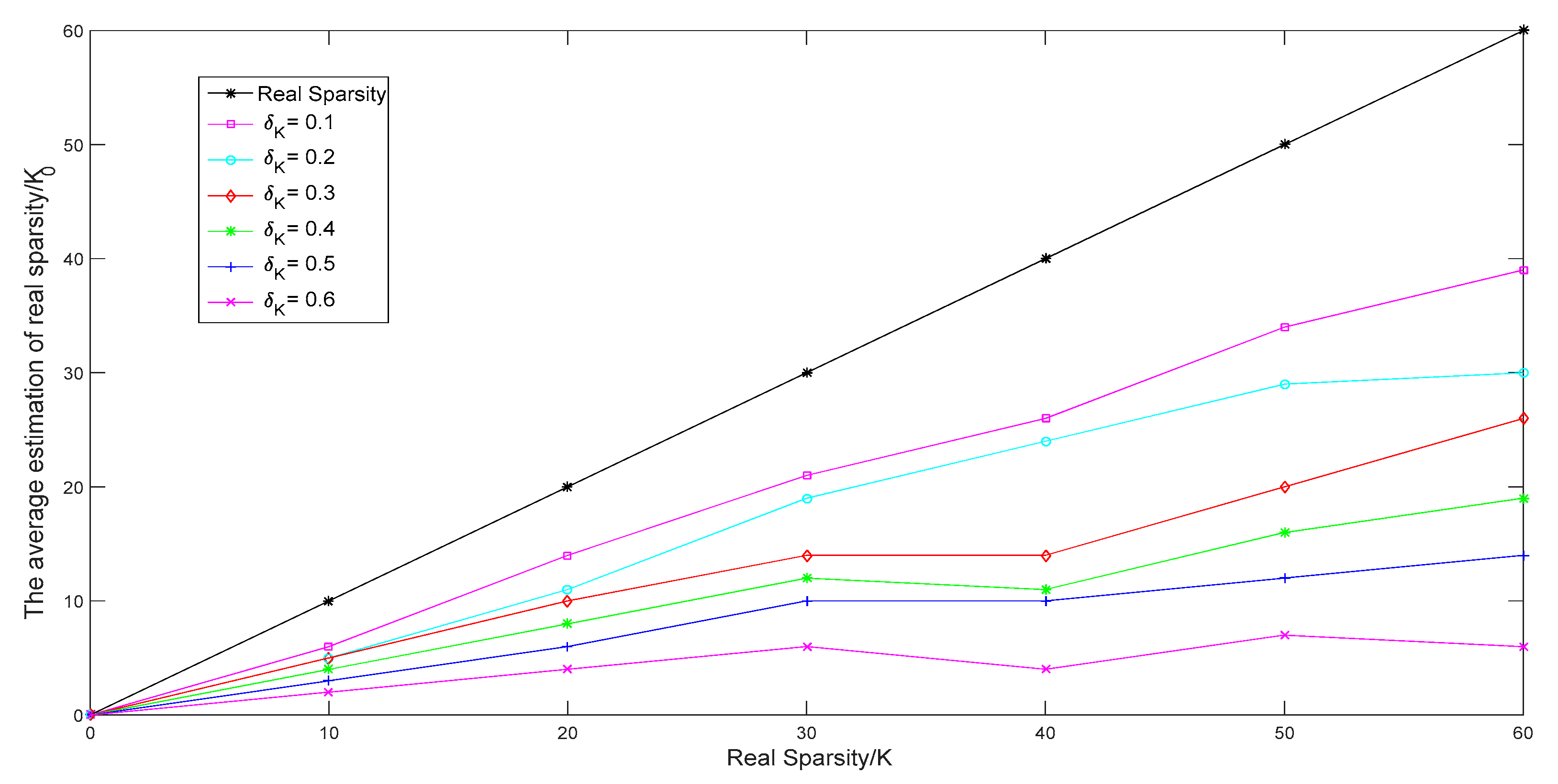
In Figure 4, we compared the average estimate of the sparsity of different isometry constants ${\delta }_K$ of the proposed method with different real sparsity $K$. We set the range of the real sparsity and isometry constant set as $K\in [10 60]$ and ${\delta }_K\in [0.1,0.2,0.3,0.4,0.5,0.6]$, respectively. From Figure 4, we can see that when the isometry constant was equal to 0.1, the estimated sparsity $K_0$ was closer to the real sparsity of the original, rather than the other isometry constant. When the isometry constant was equal to 0.6, the estimated sparsity was much lower than the real sparsity of the signal. Therefore, we can say that a smaller isometry constant may be useful for estimating sparsity. Furthermore, this indicates that a smaller isometry constant can reduce the runtime of sparsity adjustments, making the recovery algorithm able to more quickly approach the real sparsity of the signal, thereby decreasing the overall recovery runtime of the proposed method.

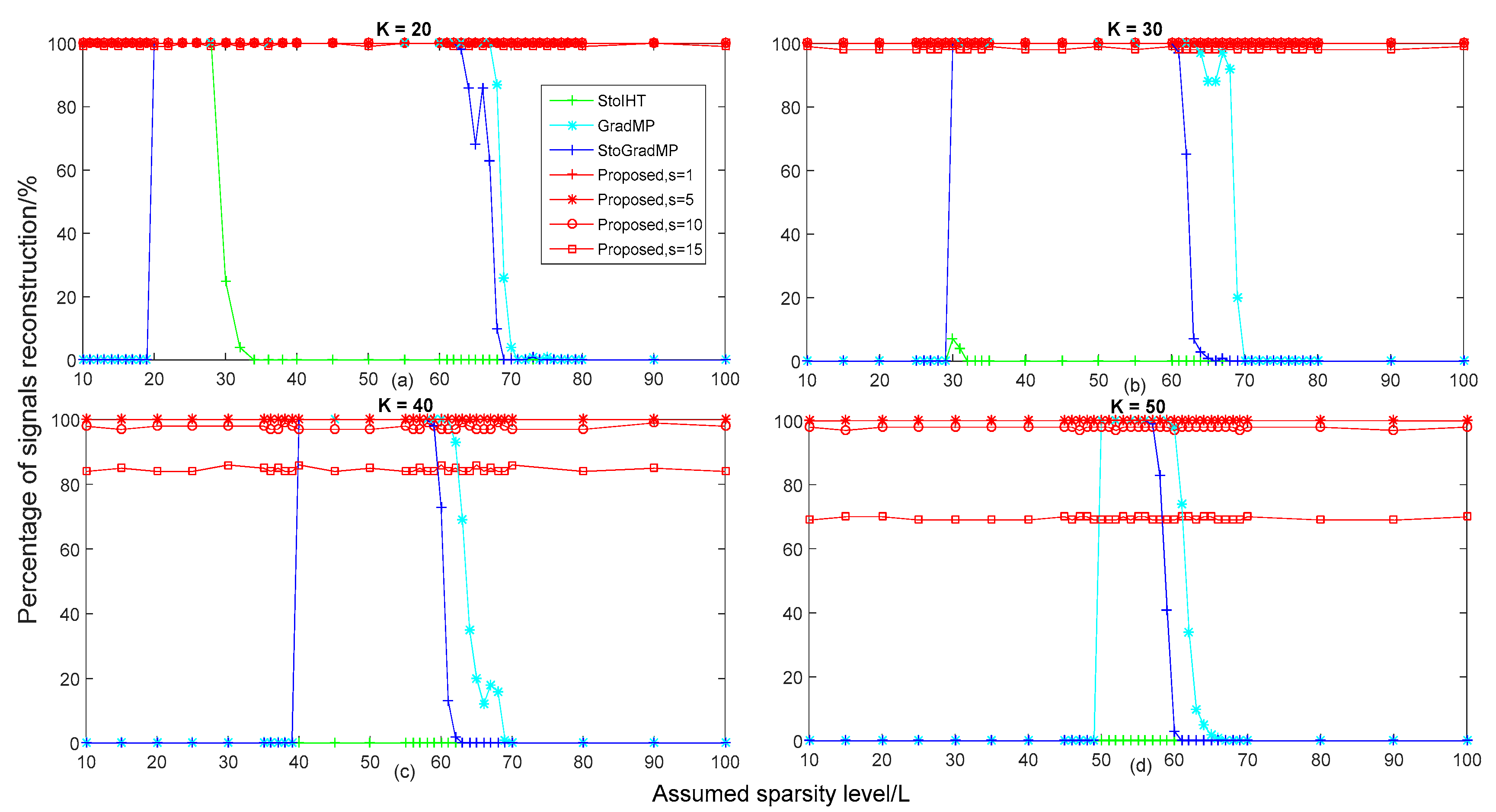
In Figure 5, we compared the reconstruction percentage of different algorithms with different sparsities in different real sparsity conditions. We set the range of the real sparsity of the original signal and the assumed sparsity as $K\in [20,30,40,50]$ and $L\in [10100]$, respectively. From Figure 4, we can see that when the isometry constant was equal to 0.1, the estimated level of sparsity was higher than the other isometry constants. Therefore, we set the isometry constant as 0.1 in the simulation in Figure 5. In Figure 5a,b, we can see that the proposed method had a higher reconstruction percentage than other algorithms when the real sparsity was equal to 20 and 30, almost all of them reached 100%. In Figure 5a, for real sparsity $K=20$, we can see that when the assumed sparsity $L<20$, the reconstruction percentage of the StoIHT, GradMP and StoGradMP algorithms was 0%, that is to say, these algorithms could not complete the signal recovery. When $20\le L\le 28$, all recovery methods almost achieved a higher reconstruction percentage. When $28\le L\le 34$, the reconstruction percentage of the StoIHT algorithm began to decline from approximately 100% to 0%, while the other algorithms still had a higher reconstruction percentage. When $34\le L$, the reconstruction percentage of the StoIHT algorithm was 0%. For $63\le L\le 72$, the reconstruction percentage of the GradMP and StoGradMP algorithms began to decline from approximately 100% to 0%. Moreover, the reconstruction percentage of the GradMP algorithm was higher than the StoGradMP algorithm in the variation range of this sparsity. In Figure 5b, we can see that the reconstruction percentage of the StoIHT algorithm was still 0% for all assumed sparsity. When $L<30$, the reconstruction percentage of the GradMP and StoGradMP algorithms was equal to 0%, while the proposed method had a higher reconstruction percentage and was approximately 100%. For $30\le L\le 61$, the reconstruction percentage of all recovery methods was approximately equal to 100%. When $61\le L\le 65$, the reconstruction percentage of the StoGradMP algorithm began to decline from approximately 99% to 1%, while the GradMP algorithm still had a higher reconstruction percentage. In Figure 5c,d, we can see that the reconstruction percentage of the proposed method with $s=15$ decreased from approximately 99% to 84% and 69%, respectively. Furthermore, from all of the sub-figures in Figure 5, we can see that when the assumed sparsity was close to the real sparsity, the reconstruction percentage of the GradMP and StoGradMP algorithms were very close, with almost no difference. In addition, when the real sparsity of the original signal gradually increased, the range of sparsity that maintained a higher reconstruction percentage became smaller. This means that the GradMP and StoGradMP algorithms were more sensitive to larger real sparsity.

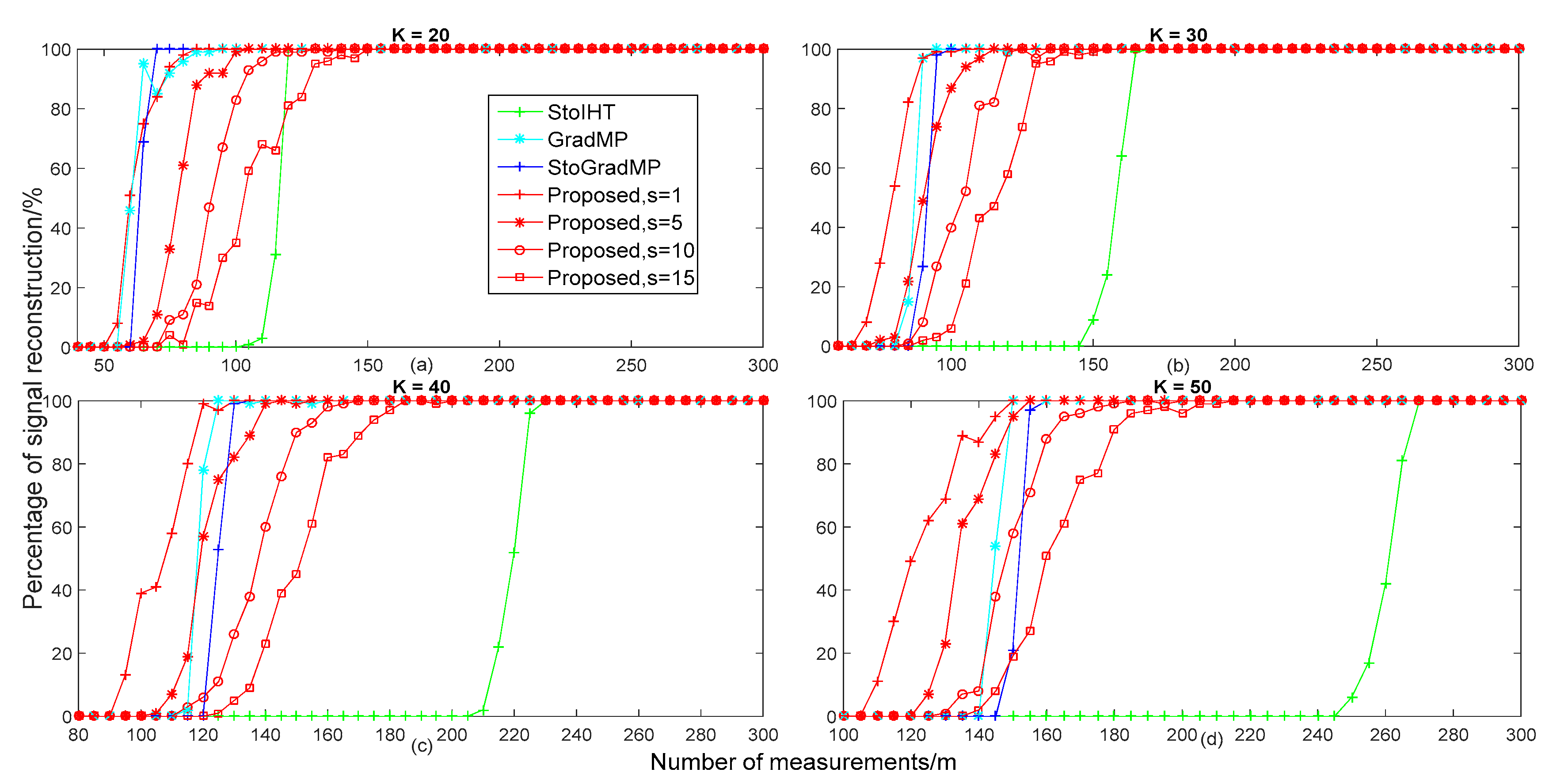
In Figure 6, we compared the reconstruction percentage of different algorithms with different measurements in different real sparsity conditions. We set the range of real sparsity as $K\in [20,30,40,50]$ in the simulation of Figure 6 to keep it consistent with Figure 5. The range of the measurement was $m=2\ast K:5:300$. From Figure 6, we can see that when the real sparsity ranged from 20 to 50, the proposed method was gradually higher than the other algorithms. In Figure 6a, we can see that when $50\le m\le 65$, the reconstruction percentage of the proposed method with $s=1$ was higher than other methods. For $65\le m\le 115$, the reconstruction percentage of the proposed method was lower than the StoGradMP and GradMP algorithms, except for the StoIHT algorithm. When $65\le m\le 145$, the reconstruction percentage that the StoIHT algorithm was superior to the proposed method was $s=15$. When $150\le m$, all of the recovery methods almost achieved higher reconstruction probabilities. In Figure 6b, we can see that when $65\le m\le 92$, the reconstruction percentage of the proposed method with $s=1$ and $s=5$ was higher than the StoGradMP and StoIHT algorithms. When $92\le m\le 165$, the recovery percentage of the proposed method with $s=5,10,15$ was higher than the StoIHT algorithm, except for the StoGradMP and GradMP algorithms. For $95\le m\le 145$, the reconstruction percentage of the proposed method with $s=5$ was higher than the proposed method with $s=10$ and $s=15$, while the StoIHT algorithm still could not complete a recovery of the signal. When $145\le m\le 165$, the reconstruction percentage of the SoIHT algorithm began to dramatically increase from approximately 0% to 100%, while the other algorithms still had a higher recovery percentage. When $165\le m$, all of the methods almost achieved higher reconstruction probabilities. In Figure 6c, we can see that when $90\le m\le 127$, the reconstruction percentage of the proposed method with $s=1$ and $s=5$ was superior to the StoGradMP and StoIHT algorithms. For $130\le m\le 185$, the recovery percentage of the proposed method with $s=5$ was higher than the proposed method with $s=10$ and $s=15$ and the StoIHT algorithm, except for the StoGradMP algorithm. In Figure 6d, we can see that the reconstruction percentage of the proposed method with $s=1$ still had a higher recovery percentage than the other methods. When $105\le m\le 153$, the reconstruction percentage of the proposed method with a random step-size was higher than the StoGradMP and StoIHT algorithms. For $110\le m\le 150$, the reconstruction percentage of the proposed method with $s=1$ and $s=5$ was higher than the other methods. When $155\le m\le 215$, the reconstruction percentage of the proposed method with $s=5$ and $s=10$ was superior to the StoIHT algorithm. When $245\le m\le 270$, the reconstruction percentage of the StoIHT algorithm ranged from approximately 0% to 100%. When $m\ge 270$, all of the methods could achieve complete recovery. Overall, based on all of the sub-figures in Figure 6, we can see that the reconstruction performance of the proposed method with $s=1$ was the best and the proposed method was more suitable for signal recovery under larger sparsity conditions.

Based on the above analysis, in a noise-free signal interference environment, the proposed method with $s=1$ and ${\delta }_K=0.1$ has a better recovery performance for different sparsity and measurements in comparison to other methods. Furthermore, the proposed method is more sensitive to larger sparsity signals. In other words, signals are more easily recovered in large sparsity environments.

In Figure 7, we compared the average runtime of different algorithms with different sparsities. From Figure 5a, we can see that the reconstruction percentage was 100% for the StoIHT algorithm with sparsity $L\in [2028]$ and the real sparsity of $K=20$ and for the GradMP, StoGradMP and the proposed method with $s=1,5,10$ with $L\in [2060]$. Therefore, we set the range of the assumed sparsity as $L\in [2028]$ and $L\in [2060]$ in Figure 7a, respectively. From Figure 7a, we can see that the average runtime of the proposed algorithm with $s=5,10$ was less than the StoGradMP algorithm, except for the proposed method $s=1$.

From Figure 5b, we can see that the reconstruction percentage of all algorithms was 100% when the range of the assumed sparsity was $L\in [3060]$ and the real sparsity was $K=30$, except for the StoIHT and the proposed method with $s=1,5$. Therefore, the range of the assumed sparsity was set as $L\in [3060]$ in the simulation of Figure 7b. From Figure 7b, we can see that the average runtime of the proposed method with $s=5,10$ was still lower than the StoGradMP algorithm.

From Figure 5c,d, we can see that the reconstruction percentage of all reconstruction methods was 100% when the assumed sparsity level was $L=\in [4058]$ and $L=\in [5056]$, respectively, except for the StoIHT and the proposed method with $s=10$ and $s=15$. Therefore, we set the range of the assumed sparsity as $L\in [4058]$ and $L=\in [5056]$ in the simulation of Figure 7c,d, respectively. From Figure 7c,d, we can see that the proposed algorithm with $s=5$ had a shorter runtime than the StoGradMP algorithm. Although the proposed method with $s=1$ had a longer runtime than the other method, it required less measurements to achieve the same reconstruction percentage as the others shown in Figure 6. Furthermore, from all sub-figures in Figure 7, we discovered that the average runtime of all algorithms increased when the assumed sparsity was gradually greater than the real sparsity, except for in the proposed method. This means that the inaccuracy of the sparsity estimation will increase the computational complexity of these algorithms. Meanwhile, it is indicated that the proposed method removes the dependence of the state-of-the-art algorithms on real sparsity and enhances the practical application capacity of the proposed algorithm.

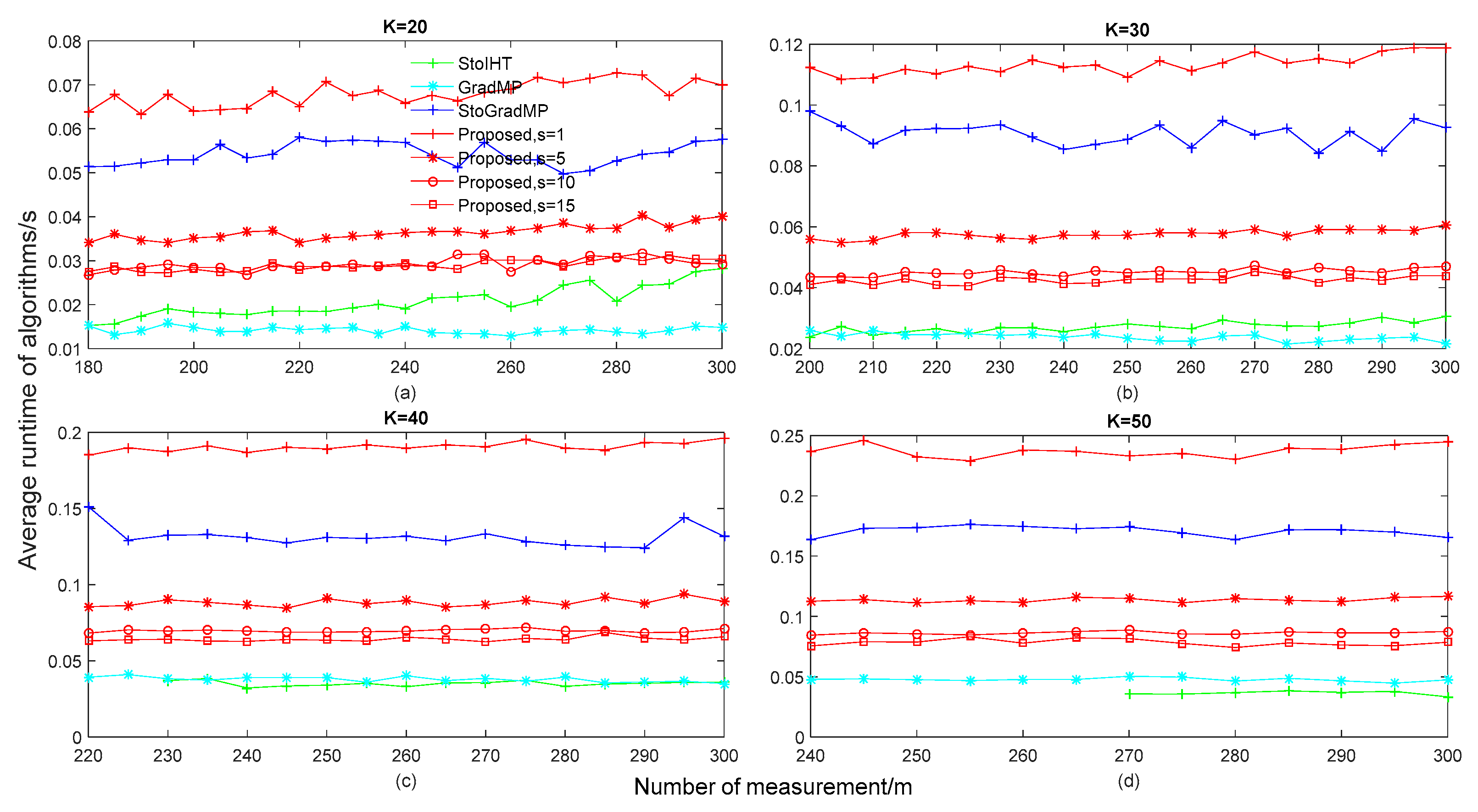
In Figure 8, we compared the average runtime of different algorithms with different measurements in different real sparsity conditions. From Figure 6, for the different sparsity levels, we can see that all algorithms could achieve 100% reconstruction when the number of measurements was greater than 180, 200, 220 and 240, respectively, except for the StoIHT algorithm. Therefore, we set the range of measurements as $m\in [180300]$, $m\in [200300]$,$m\in [220300]$, and $m\in [240300]$ in Figure 8a–d, respectively. In particular, in Figure 6c,d, we can see that the reconstruction percentage was 100% when the number of measurements of the StoIHT algorithm was greater than 230 and 270, respectively. Therefore, we set the range of measurements as $m\in [230300]$ and $m\in [270300]$ in the simulation of Figure 8c,d, respectively.

From Figure 8, we can see that the GradMP algorithm had the lowest runtime, the next lowest were the StoIHT algorithm, the proposed algorithm with $s=5,10,15$ and the StoGradMP algorithm. This means that the proposed method with $s=5,10,15$ had a lower computational complexity than the StoGradMP algorithm, except for the GradMP and StoIHT algorithms. Meanwhile, in terms of the proposed algorithm, we can see that when the size of the step-size was $s=15$, the average runtime was the shortest, the next shortest were the proposed method with $s=10$, the proposed method with $s=5$ and the proposed method with $s=1$, respectively. This shows that a larger step-size will be beneficial to approach the real sparsity $K$ of the original signal, thereby reducing the computational complexity of the proposed method. Furthermore, from Figure 6 and Figure 8, although the proposed method with $s=1$ had the highest runtime, it could achieve reconstruction with fewer measurements than the other algorithms.

Based on the above analysis, in a noise-free signal interference environment, the proposed algorithm had a lower computational complexity with a larger step-size than a smaller step-size. Although, the proposed method had a higher computational complexity than some existing algorithms in some conditions, it is more suitable for applications without knowing the sparsity information.

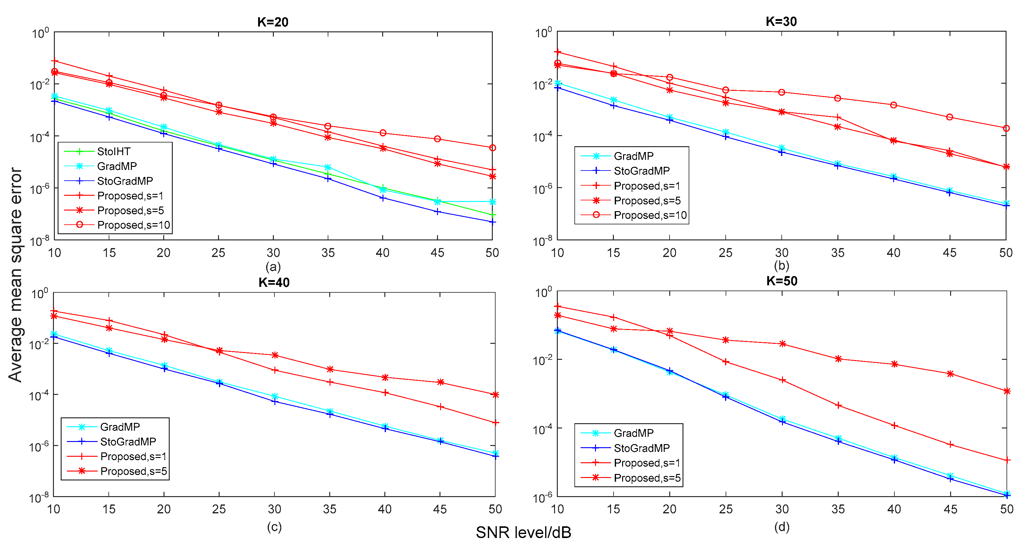
In Figure 9, we compared the average mean square error of different algorithms with different $SNR$ levels in different real sparsity conditions to better analyze the reconstruction performance of the different algorithms when the original sparse signal was corrupted with different levels of noise. We set the range of the noise signal level as $SNR=10:5:50$ in simulation of Figure 9. Furthermore, to better analyze the reconstruction performance of all reconstruction algorithms in different real sparsity levels conditions, we set the real sparsity level $K$ as 20, 30, 40 and 50, respectively. Here, the noise signal was a Gaussian white noise signal. In particular, all of the experimental parameters were consistent with Figure 5. In Figure 5a,b, the reconstruction percentage of the proposed method was 100% with a step-size of $s=1,5,10$. Therefore, we set the size of $s$ as 1, 5 and 10 in the simulation of Figure 9a,b, respectively. In Figure 5c,d, the reconstruction percentage of the proposed method was 100% with a step-size of $s=1,5$. Thus, we set the size of the step-size of the proposed method as 1 and 5 in Figure 9c,d, respectively.

From Figure 9, we can see that the proposed methods with different step-sizes had a higher error than other algorithms for different $SNR$ levels. This is because the proposed methods supposed that the sparsity prior information of the source signal was unknown, while the other methods used the real sparsity as prior information. The estimated sparsity by our proposed method was still different to the real sparsity. This made the proposed method have a higher error than the others. In particular, the error was very small for all algorithms with a larger SNR, which had little effect on the reconstruction signal. Although the proposed method was inferior to other algorithms in terms of reconstruction performance when the original sparse signal was corrupted by different levels of noise, it provides a reconstruction scheme that is more suitable for practical applications. In this paper, we mainly focused on the no noise environments. Recently, in Reference [33,34,35,36], the researchers focused on the reconstruction solutions for the original signal in the presence of noise corruption and several algorithms were proposed. In the future, we can use their ideas to improve our proposed method in anti-noise interference performance.

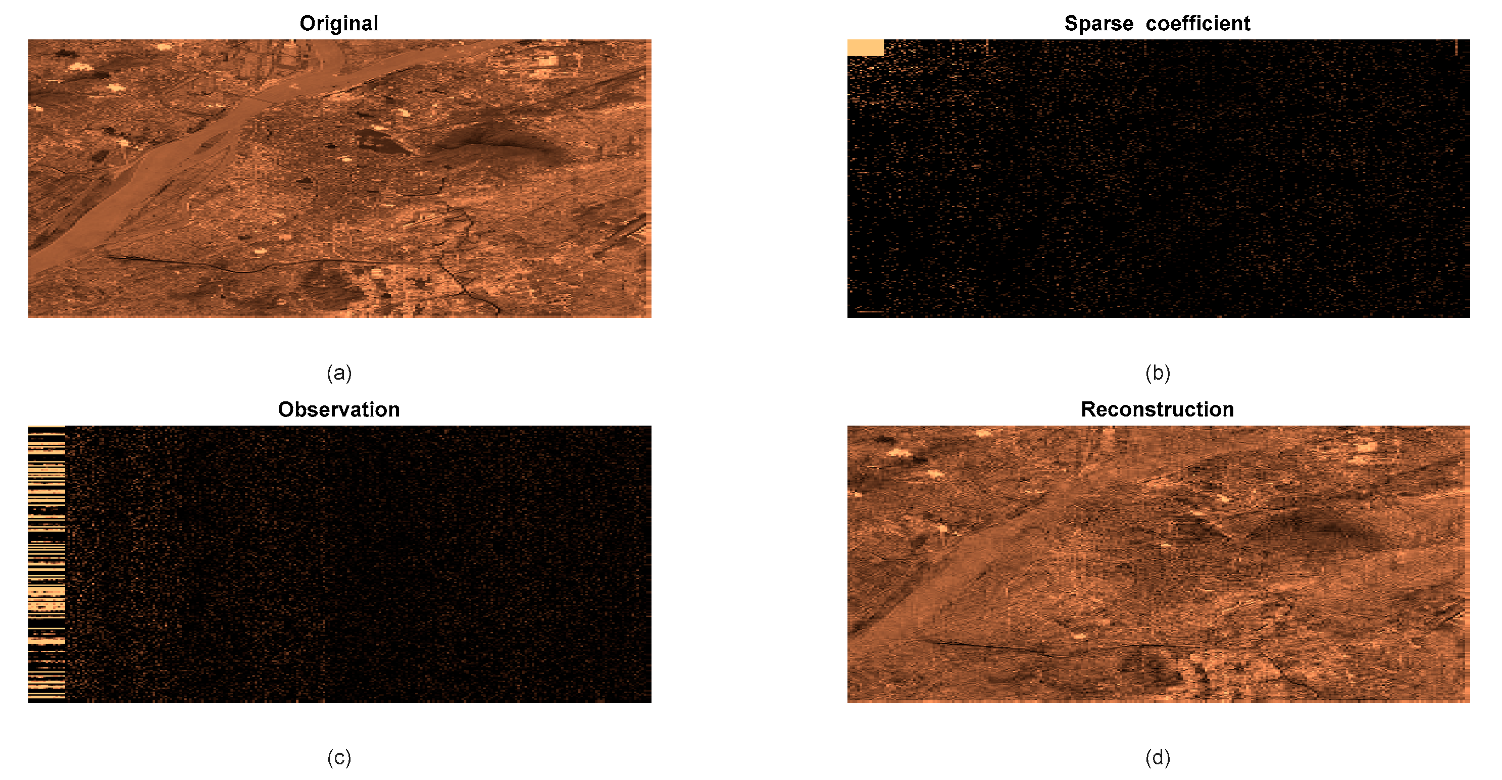
In Figure 10, we test the application efficiency of our proposed method in remote sensing image compressing and reconstructing. The Figure 10a–d show the original remote sensing image, its sparse coefficient, compressed image(observation signal) and reconstructed image by our proposed method. By comparing the Figure 11a with Figure 10d, we can see that our proposed method reconstructs the compressed remote sensing image successfully.

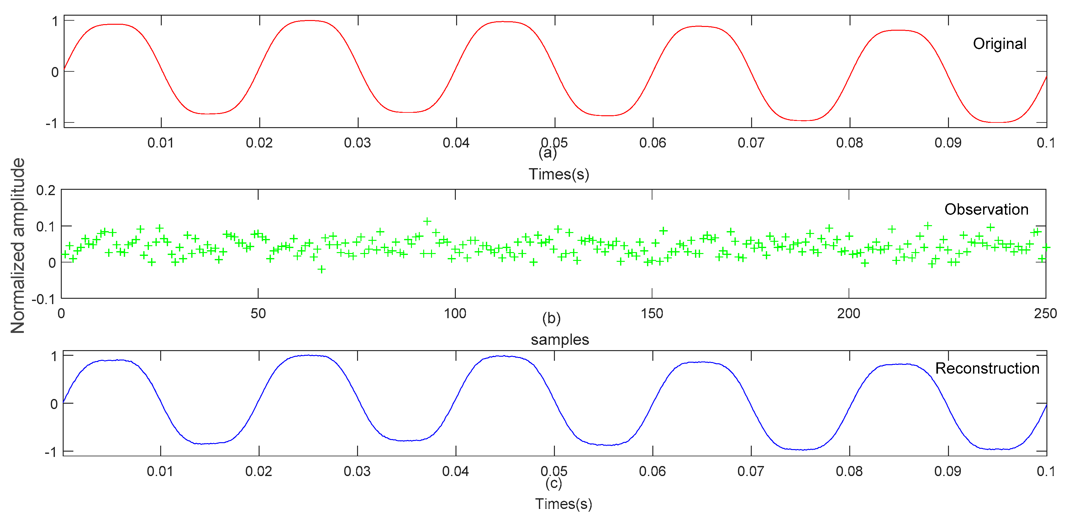
In Figure 11, we test the efficiency of our proposed method in application of power quality signal compressing and reconstruction. The Figure 11a–c show the inter-harmonic signal, compressed signal (observation signal) and reconstructed inter-harmonic signal by our proposed method respectively. It can be seen from Figure 11a,c that the waveforms of two figures are basically the same. This proves that our proposed method is efficiency for inter-harmonic reconstruction.

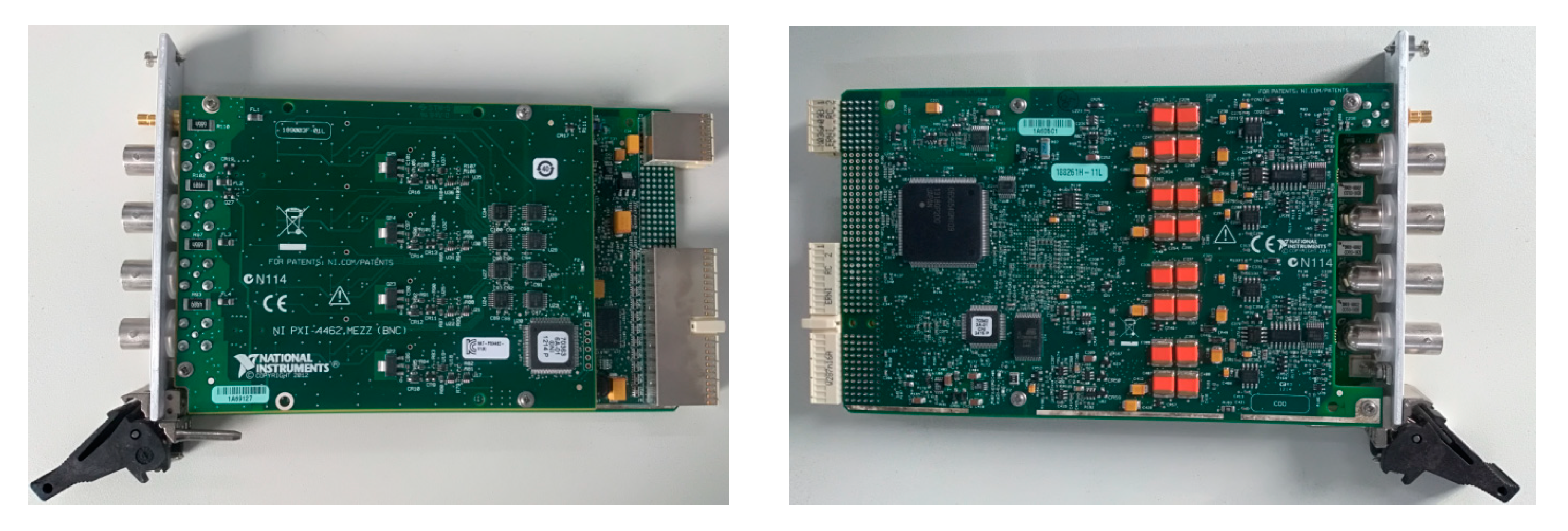
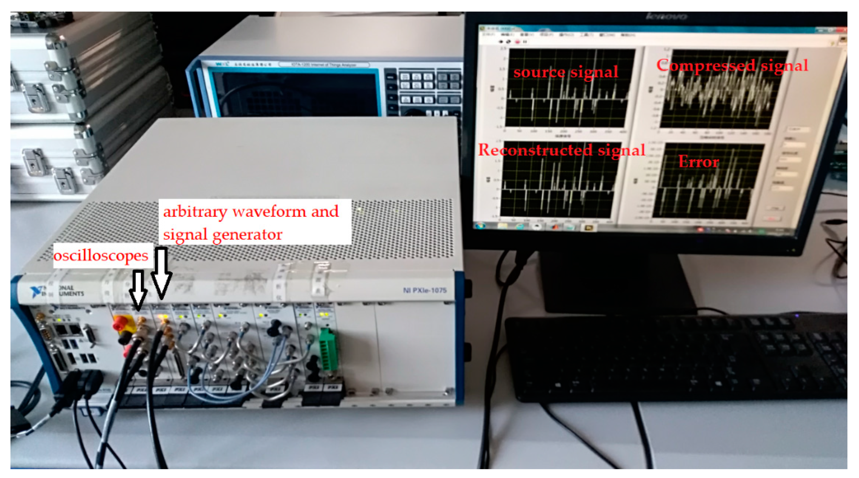
We also used the National Instruments PXI (peripheral component interconnect extensions for instrumentation) system to test the efficiency of our proposed method in application. The hardware of the PXI system includes an arbitrary waveform and signal generator and oscilloscopes. The hardware architecture of arbitrary waveform and signal generator is shown in Figure 12. The hardware architecture of oscilloscopes is shown in Figure 13. 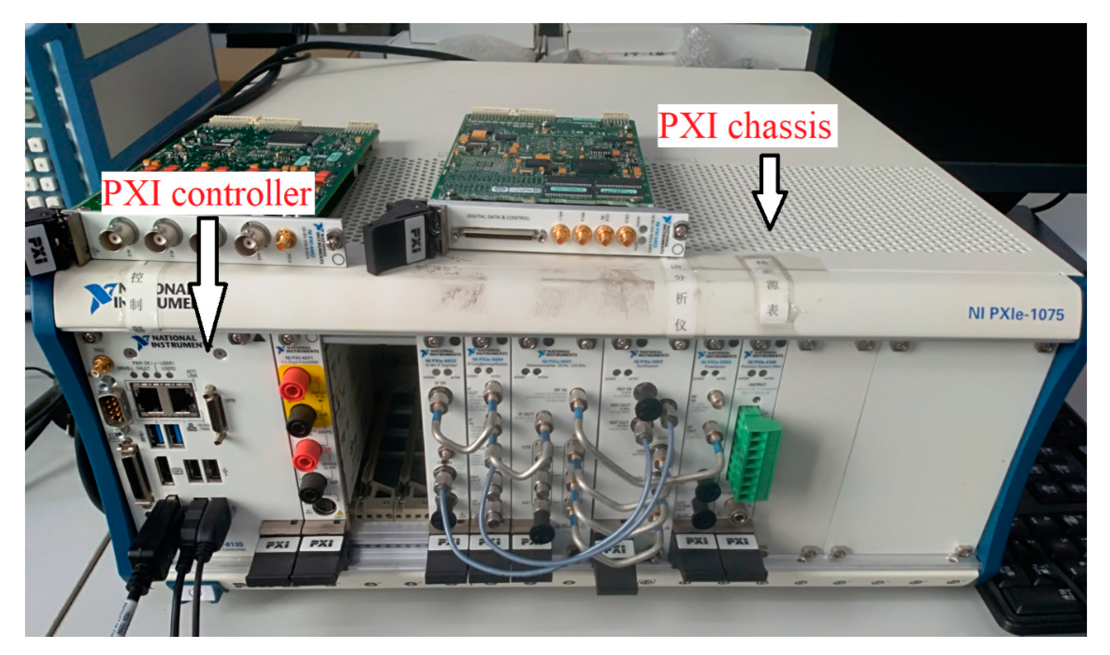Figure 14 shows the PXI chassis and controller, which are used to control the arbitrary waveform and signal generator and oscilloscopes. We insert the arbitrary waveform and signal generator and oscilloscopes into PXI chassis to construct the complete measurement device. As is shown in Figure 15. Mixed programming of Labview and MATLAB were used to realize the compressed and reconstructed algorithm. From the experimental results, it can be seen that the proposed method successfully reconstructed the source signal from the compressed signal.

7. Conclusions

This paper proposed a new recovery method. This method first utilized the sparsity pre-evaluation strategy to estimate the real sparsity of the original signal and used the estimated sparsity as the length of the support set in the initial stage, which allows the proposed method to eliminate the dependency of sparsity, thereby reducing the computational complexity of the proposed method. The proposed algorithm then adopts the adjustment strategy of sparsity estimation to control the convergence of the proposed method and adjust the estimated sparsity, which makes the proposed method more accurately approach the real sparsity of the original signal. Furthermore, a reliability verification condition was added to ensure the correctness and effectiveness of the proposed method. The proposed method not only solved the problem of the sparsity estimation of the original signal but also improved the recovery performance of the practical applications of the proposed method. The simulation results proved that the proposed method performed better than other stochastic greedy pursuit methods in larger sparsity environments and smaller step-sizes.