DC-Microgrid System Design, Control, and Analysis

Abstract

Recently direct current (DC) microgrids have drawn more consideration because of the expanding use of direct current (DC) energy sources, energy storages, and loads in power systems. Design and analysis of a standalone solar photovoltaic (PV) system with DC microgrid has been proposed to supply power for both DC and alternating current (AC) loads. The proposed system comprises of a solar PV system with boost DC/DC converter, Incremental conductance (IncCond) maximum power point tracking (MPPT), bi-directional DC/DC converter (BDC), DC-AC inverter and batteries. The proposed bi-directional DC/DC converter (BDC) lessens the component losses and upsurges the efficiency of the complete system after many trials for its components’ selection. Additionally, the IncCond MPPT is replaced by Perturb & Observe (P&O) MPPT, and a particle swarm optimization (PSO) one. The three proposed techniques’ comparison shows the ranking of the best choice in terms of the achieved maximum power and fast—dynamic response. Furthermore, a stability analysis of the DC microgrid system is investigated with a boost converter and a bidirectional DC-DC converter with the Lyapunov function for the system has been proposed. The complete system is designed and executed in a MATLAB/SIMULINK environment and validated utilizing an OPAL real-time simulator.

1. Introduction

A microgrid is a small-scale grid system that can work freely or in conjunction with the region’s principal electrical grid. Today, the microgrid is picking up a considerable measure of desirability since new renewable energy sources that occasionally work better nearer to the point of cause, are instead connected to the main electrical grid. The best illustration is a photovoltaic system [1,2,3]. Nowadays, more houses and structures are associated with the small neighborhood solar energy grid frameworks that may serve only one property. Besides, as solar innovation descends in cost and turns out to be more viable, a few features can really get advantageous by a smaller economy of scale—straightforward solar cells put in accessible territories can take in free regular daylight and be changed it over to electrical energy to run a specific arrangement of machines or warming and cooling frameworks. The microgrid alludes to a small-scale power grid that can keenly succeed in managing energy exchange between the interconnected loads and the distributed generation sources, for example, photovoltaics (PVs) [4]. Microgrids can be proposed as backup power generation or to support the principle electrical grid amid times of substantial demand. Frequently, microgrids include different energy sources as a method for consolidating sustainable power. Different purposes incorporate lessening costs and upgrading reliability. There are two fundamental sorts of microgrid; direct current (DC) microgrid and alternating current (AC) microgrid. Figure 1 demonstrates a schematic perspective of the DC microgrid system. This framework uses a DC bus as its primary support and allocates power to a group that comprises a few handfuls or a hundred family units in a neighborhood. Solar cells, fuel cells, batteries, etc., are the energy sources of a DC microgrid to deliver power to loads. To change DC voltages to the rated DC voltage, a buck or boost converter has been utilized in the microgrid. To uphold reference output voltage, a DC-DC converter is controlled by a proportional integral (PI) controller.

Recently, renewable energy sources have gained a lot of attraction because of high energy demand, changes in natural strategies, and the scattered populace around the world. The concern of the environmental changes is driving in significant variations in power generation and utilization designs. Different nations have set the objective of reducing 20% of greenhouse gas by 2020. These natural concerns have pulled in broad consideration to move towards more earth benevolent energy sources, for example, a photovoltaics (PV) system, wind turbines, and fuel cells. However, these energy sources are directly dependent on the environment, for example, in PV systems, there are changes in the radiation of sunlight and temperature. The power produced from these sources fluctuates, which effects inversely to the main power grid. The ideal approach to shield this issue is to move towards a more astute confined framework such as a microgrid (MG). A microgrid can work in an islanded mode when there are blackouts for supplying power to local loads. A microgrid can likewise function as backup power when there is a lack of supply from the main grid. Point of common coupling (PCC) makes the connection between the microgrid and the main grid. Additionally, both the PV systems and the fuel cells produce direct current (DC) whereas the infrastructure of the exciting power generation system is based on alternating current (AC). While integrating these renewable energy systems with the present structure, this DC voltage must be changed to AC, utilizing converters which include additional transformation steps that lead to upsurge power losses, thus diminishing general framework proficiency [5,6]. In fact, there are countless DC loads, for example, PCs, servers, mobiles, TVs and so on that require another step to convert this AC power to DC, bringing on additional losses. Different modeling techniques for a photovoltaic cell utilizing Matlab/Simulink/Simscape are proposed [7]. However, maximizing the power point via efficient tracking technique is still one of the important research points to be addressed [8,9,10], associated with efficient various DC microgrids control [11,12,13,14,15]. The real issue with the current solar energy MPPT technology is that the productivity of the PV system is still low and does not work at its best effectiveness relating to the nonlinear varieties [16,17]. DC microgrid has the ability of conversion losses reduction on the demand side [18]. The upcoming microgrid will be a crucial part of the distribution power system to accessible assimilate different types of distributed generation sources [19]. In addition, the growing load such as consumer electronics, power storage, and solar modules are essentially DC in nature, more DC microgrids and hybrid ones will likewise act in the distribution power system [20,21]. However, the evolving concept of DC microgrid needs more investigation on power flow analysis. One of the proposed methods is to model the DG (Distributed-Generation) sources and components as droop buses. In a DC microgrid, the load allocation mechanism is accomplished by droop control by feeding back the output current via a virtual resistance to the voltage loop. The optimization of demand response at the residential side and DC microgrid in the process phase is adopted as well. One of the approaches to enhance the system efficiency is to coordinate the storage devices and/ or the loads [22,23,24].

PV systems cannot be demonstrated as a steady DC source since its output power relies upon the load current, temperature, and insolation. For the most part, maximum power point tracking (MPPT) is received to track the maximum power point in the PV framework. The productivity of MPPT relies upon both the MPPT control algorithm and the MPPT circuit. The MPPT control algorithm is generally connected in the DC-DC converter that is regularly utilized as the MPPT circuit. From the seventies, a remarkable number of MPPT control strategies have been proposed starting with basic (for example, voltage and current input based MPPT) to more enhanced power based MPPT (for instance, the P&O procedure and the incremental conductance strategy) methods. As of late intelligent based plans have been presented.

The maximum power point tracking (MPPT) is a vital part for the photovoltaic (PV) system to always get the maximum extracted power from the system. However, it is not an easy task because of the extensive variations in exterior effects and the nonlinear association of the electrical characteristics of the PV panels. Up to now, there are different MPPT methods based on control approaches engaged and climate circumstances. These various methods could be classified between online, offline, and intelligent techniques such as incremental conductance (IncCond), perturb and observe (P&O), neural networks (NN), fuzzy logic (FL), and constant voltage (CV). Some of these techniques like P&O, have a drawback that the fluctuations generation nearby the MPP (Maximum-Power_Point), slow tracking speed, and loss of a substantial quantity of energy in the control unit. The IncCond technique has been established to overwhelmed P&O issues for better efficiency and faster response. However, the recent research into MPPT methods are proposing the dynamic behavior’s enhancement over the traditional techniques [25,26,27]. Modern models for PV modules based on neural networks is implemented with performance enhancement utilizing a genetic algorithm (GA) [28,29,30]. Various duty cycles values for DC-DC converter have been estimated using NN, [31] for MPPT, then utilized in a stand-alone PV system with its converter and inverter modeling [32,33]. MPPT algorithm with photovoltaic array emulator using DC/DC converters has been investigated [34]. PV panels’ position adjustment has been adopted to reduce line losses [35]. The P&O and IncCond methods have been used for MPPT under dynamic weather conditions [36]. P&O technique combined with particle swarm optimization (PSO) for MPPT is implemented [37,38] and also IncCond technique utilized PSO for a standalone PV system to enhance its dynamic performance [39]. A modern approach for MPPT modeling validation is to use the real-time simulator or the hardware-in-the-loop (HIL) apparatus as shown in references [40,41]. A novel MPPT algorithm on PSO for PV systems is implemented and validated by the OPAL-real-time simulator by one of the authors [42].

The objective of this paper is to investigate, model, and design a complete standalone solar PV system with DC microgrid. The system is designed to feed a fixed DC load of 1 kW and fixed AC load of 8 kW, 500 kVAR load which can be assumed as a small area that can be powered from this standalone DC microgrid without depending on the main grid connections. To enhance the PV array efficiency, a PSO (Particle-Swarm-Optimization) MPPT (Maximum-Power-Point-Tracking) technique has been utilized to track the maximum power from a PV panel for a nano-grid system incomparable with the IncCond and P&O technique. The simulated system is validated by OPAL real-time simulator (HIL, Hardware-In-the-Loop). The final step is to analyze the stability of the DC microgrid system with the Lyapunov function identification.

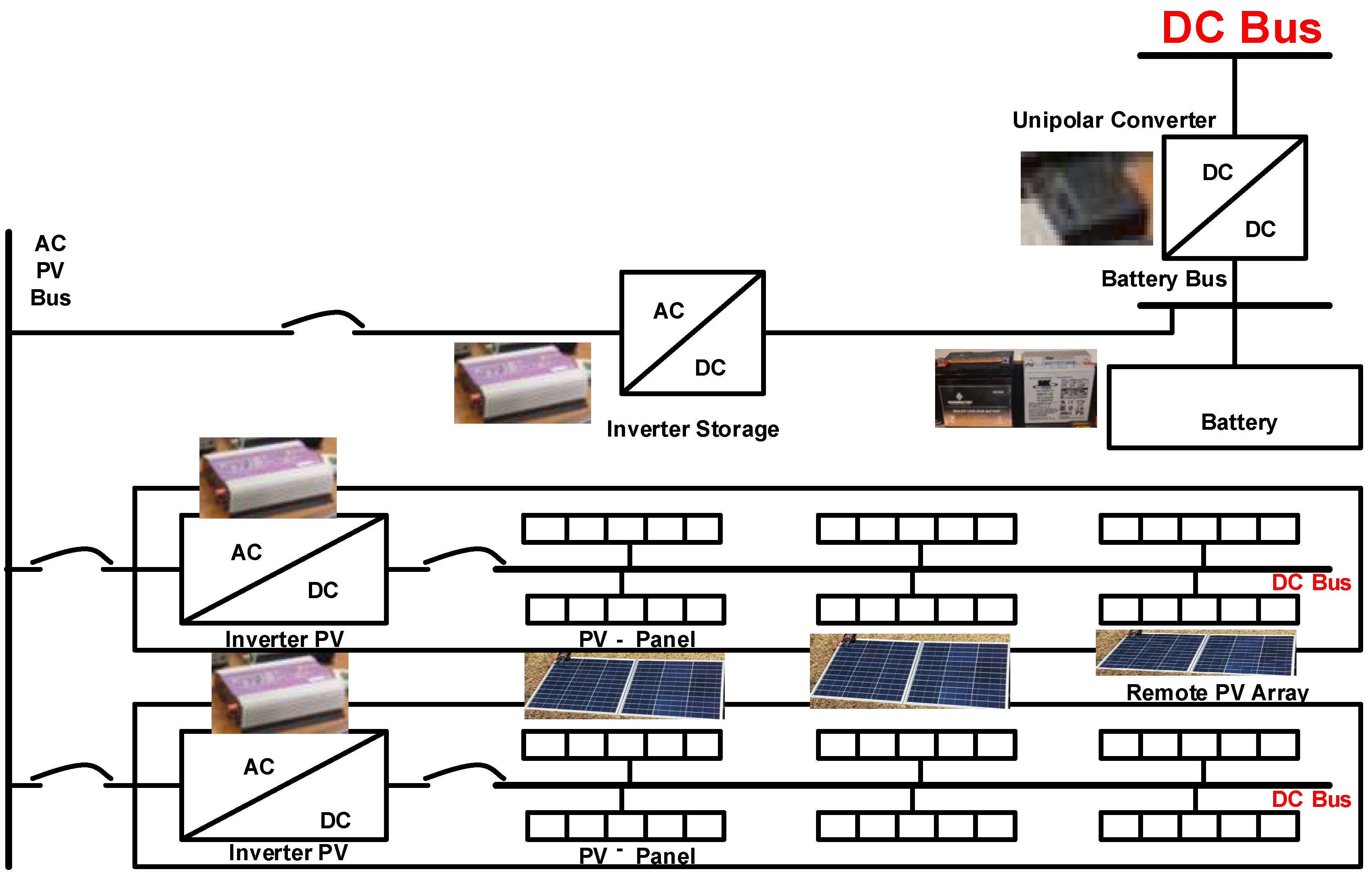
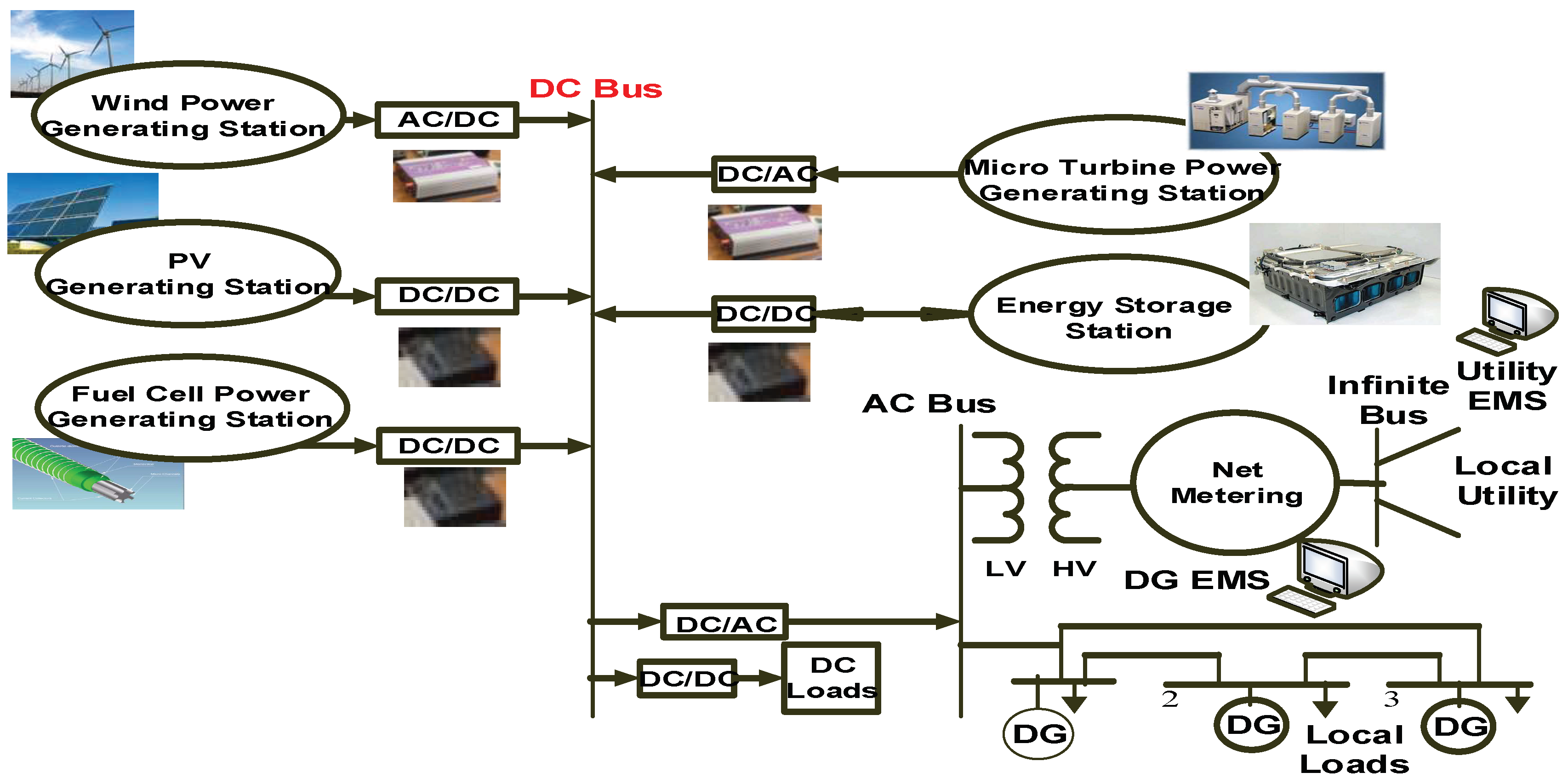
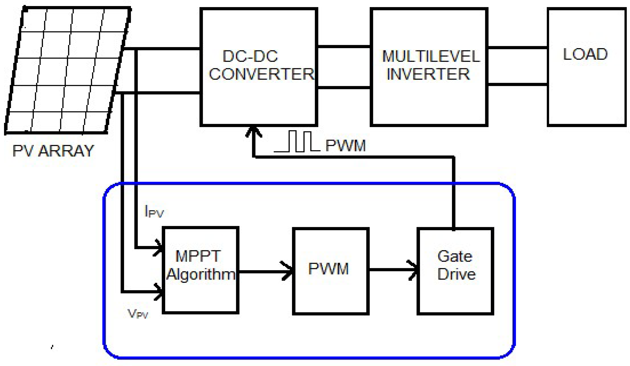
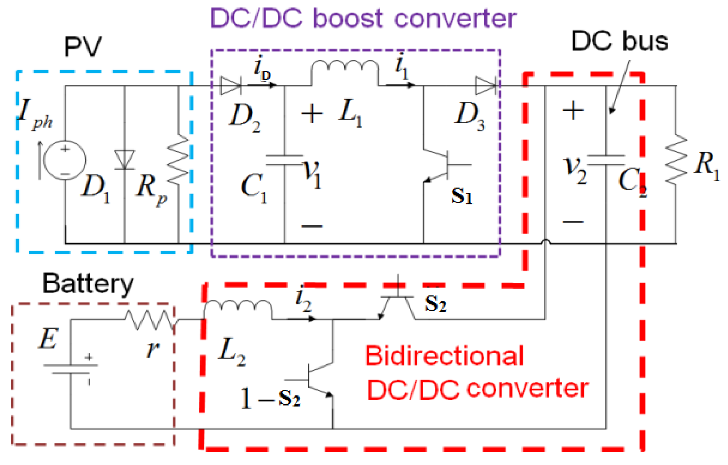
2. Photovoltaic DC Microgrid System

This proposed system consists of a PV system with incremental conductance MPPT, a DC-DC boost converter, bi-directional DC-DC converter and control circuits, DC-AC inverter and controller and a battery bank. The proposed converter decreases the component losses and upsurges the performance of the complete system with better dynamic response and maximum power by utilizing particle swarm optimization. A simple diagram of the complete system is shown in Figure 2, and this proposed system has been designed and implemented in MatLab/Simulink. Perturb and observe, incremental conductance, and particle swarm optimization MPPT approaches are compared to show the validity of the proposed PSO over the other two techniques. The OPAL real-time simulator is used to validate the PV Simulink environment with the previous comparison.

Sunlight has been converted to DC power by the solar cells. The photovoltaic cell produces electricity from the sun. At the point when PV panels are visible to daylight, it changes the sunlight or solar energy into electrical energy. The PV array is a mixture of parallel and series photovoltaic cells. This cluster builds up the power from the sunlight/solar energy in a straightforward manner, and it changes when the temperature and irradiances changes.

In Figure 3, a block diagram of a PV system has been shown. PV systems consist of an MPPT algorithm for tracking the maximum power from PV panels, DC-DC converter (boost converter) to boost the voltage of PV to rated voltage, finally, through the inverter, it connects with the loads.

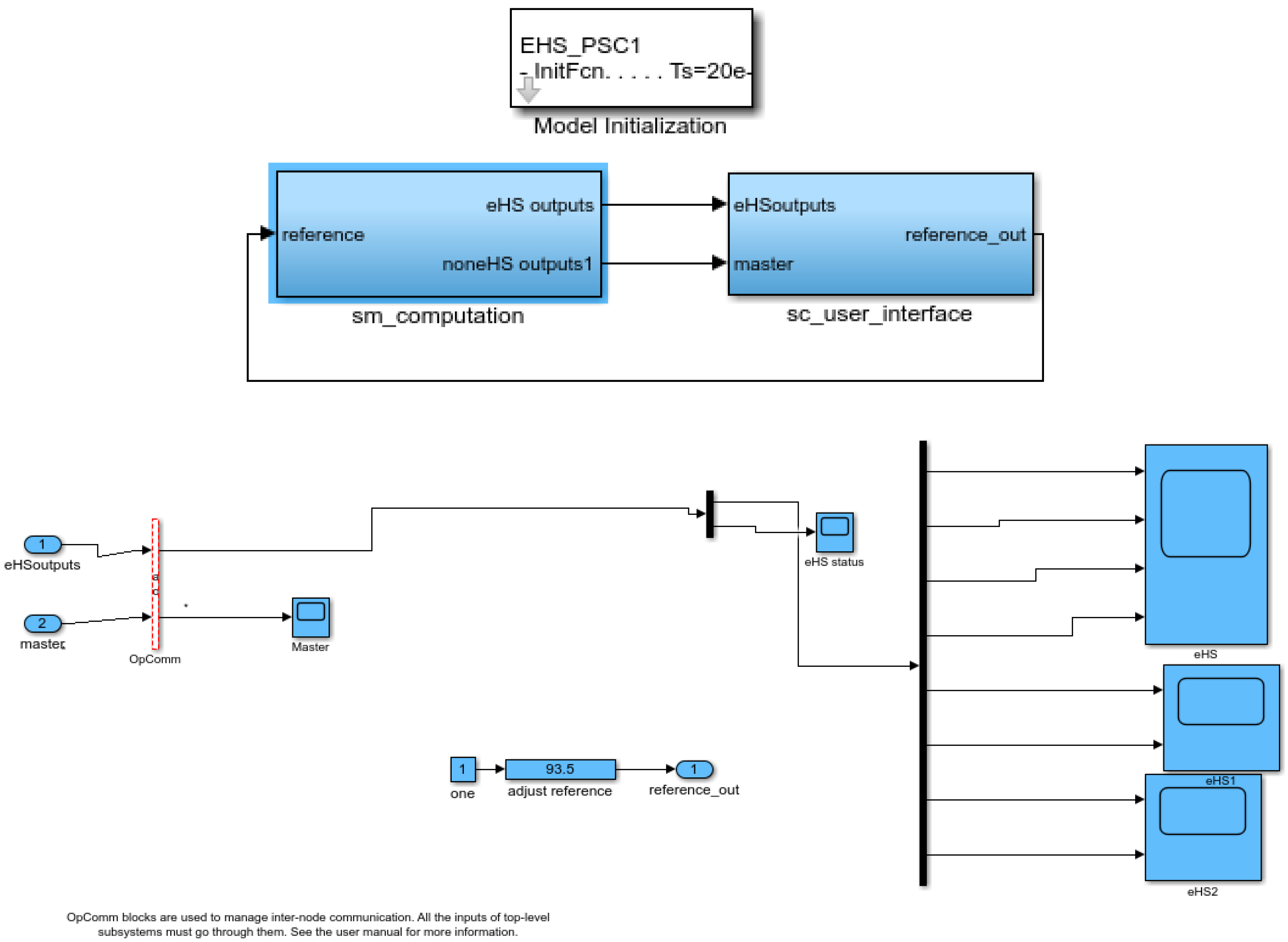
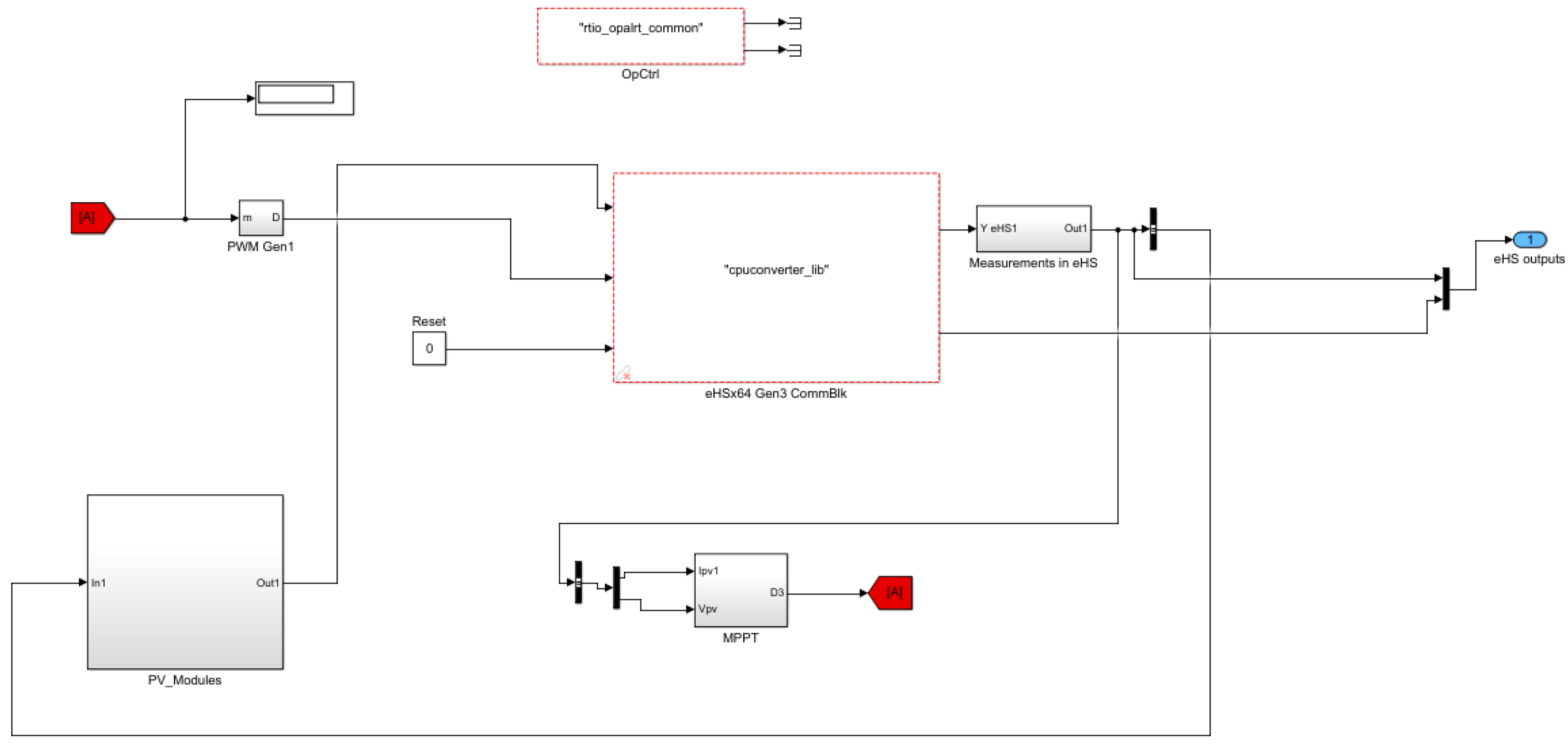
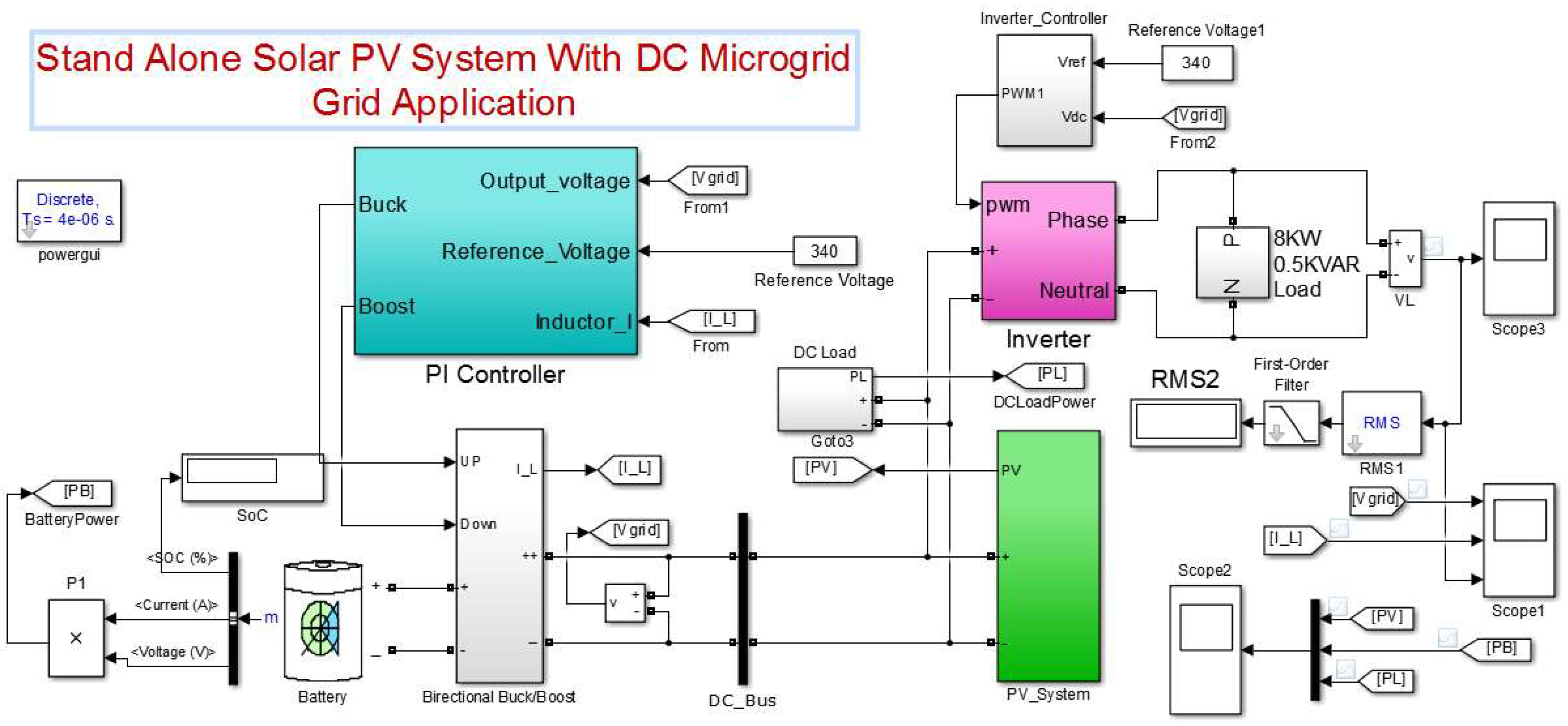
3. Simulink Representation of the Complete PV System and the Proposed MPPT Techniques

The complete system is shown in Figure 4. It compromises the PI controller for buck/ boost DC-DC converter, battery storage, inverter with its controller, PV model with its MPPT, bidirectional converter, AC and DC loads. The IncCond MPPT is replaced one time by P&O to see the advantage of the first approach, and then replaced by the PSO one for better dynamic performance as shown in the comparison figure with the aid of the HIL. The details of each element along with the proposed techniques are explained in this section in the form of flowcharts.

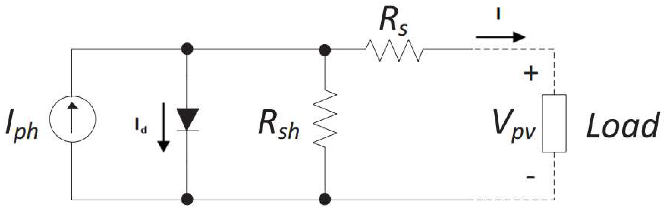
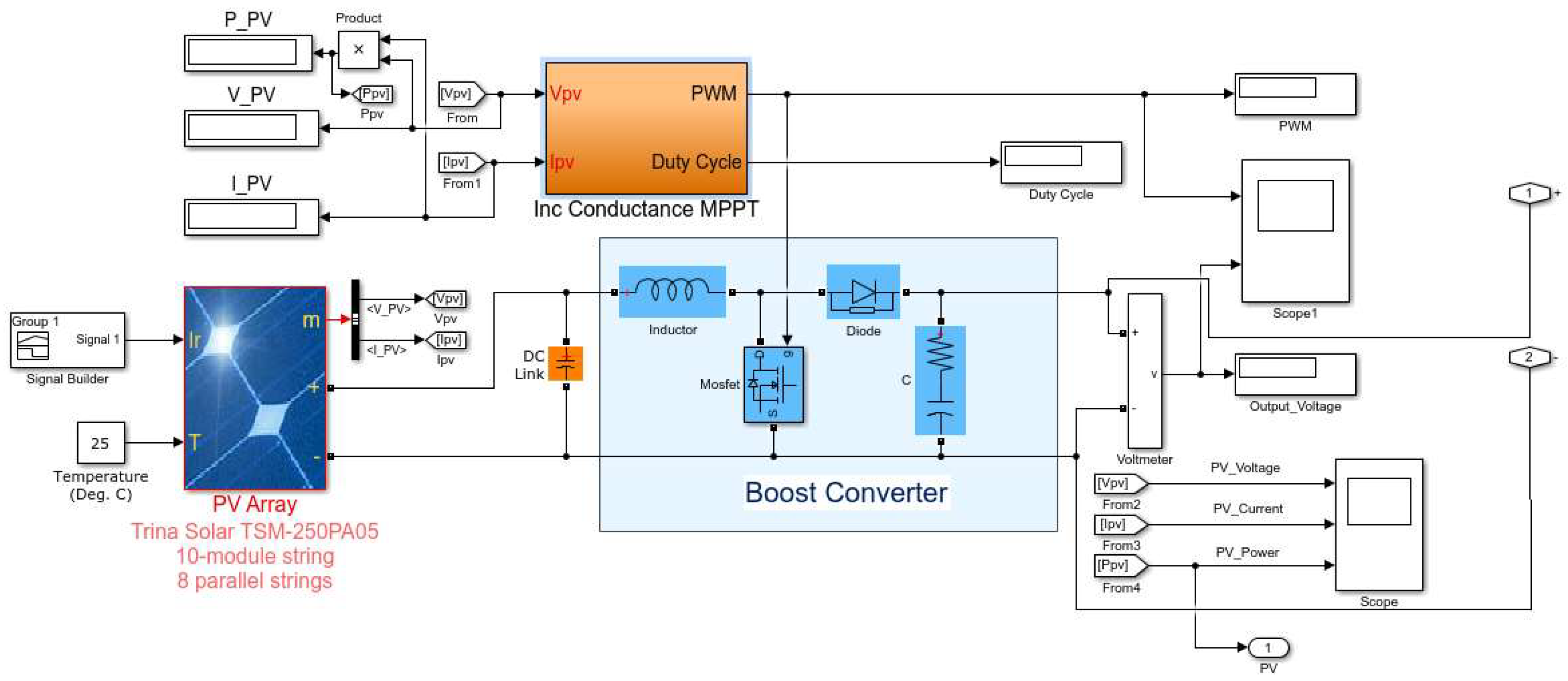
3.1. Modeling of the Solar PV System

A solar PV array can be modeled in three diverse ways by utilizing MatLab/Simulink. One of the techniques is by modeling the part that utilizes numerical expressions. The following technique is to utilize the library block of Simpower frameworks, where a PV array can be modeled by gathering PV modules as indicated by the required power output. The third strategy is the utilization of the solar cell block from the slim electronics library. The distinction between this technique and the first is that in this strategy the solar cell block contains the numerical expression [7]. In our model, we have considered the solar array block from the Simpower systems library which was established by NREL, USA. The PV array block in the Simpower frameworks is a five-parameter model which utilizes a current source driven by the sunlight in parallel with a diode, a shunt resistor, and a series resistor are linked at the output as shown in Figure 5.

The diode I-V Characteristics I_d is

$$I_d=I_0\left(exp\left(V_d/V_T\right)-1\right)$$

(1)

$$V_T=K_B\frac{T}{q}{n}_i{N}_{Cell}$$

(2)

where K_B = Boltzmann’s contact; $q$ = electron charge; I_d = diode current (A); V_d = diode voltage (V); I₀ = diode saturation current (A); T = Cell temperature (K); n_i = Diode ideality factor; and N_cell = Number of cells connected in series.

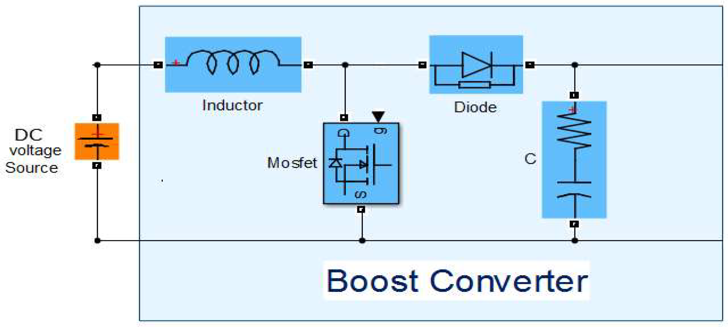
3.2. Modeling and Simulation of the Boost Converter

A boost converter has been made utilizing a capacitor, an inductor, a diode, and a switch that appears in Figure 6. The operating system of a boost converter can be clarified in two modes. The main component of the boost converter is the switching transistor. It turns some portion of a circuit on and off rapidly. Normally the speed of the switching can be more than 1000 times each second.

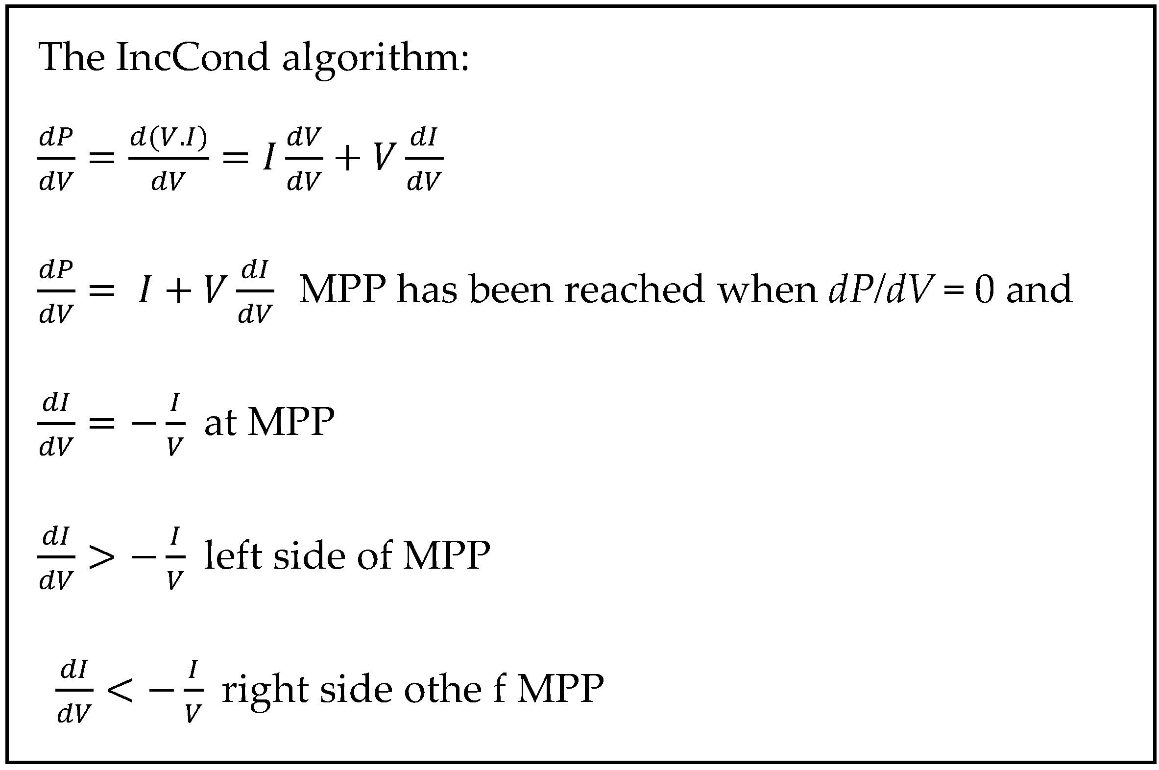
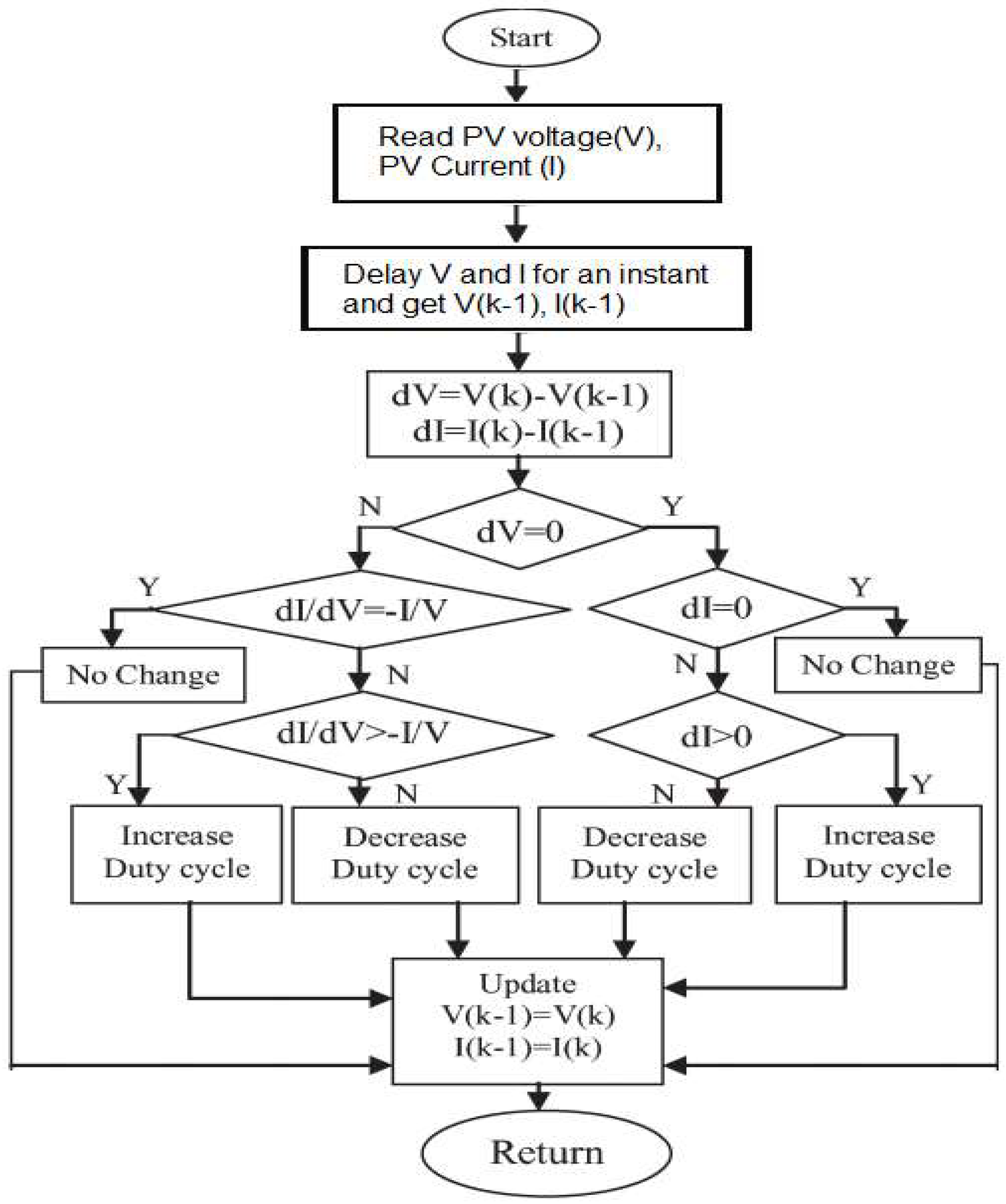
3.3. Incremental Conductance MPPT

The photovoltaic output voltage is fundamentally a component of atmospheric factors, for example, temperature and insolation. Incremental Conductance was planned considering a perception of P-V characteristic curve. This algorithm was produced to defeat some downside of the Perturb and Observe (P&O) algorithm (Figure 7). The impediment of the perturb and observe technique to track the peak power under the quick fluctuating climatic condition is overcome by the IC (Incremental-Conductance) technique. The IC algorithm is the most ordinarily utilized technique since its outcomes can be figured rapidly, and its control is effortlessly executed. The IC can verify that the MPPT has come to the MPP and quit perturbing the working point.

The MPP can be computed by utilizing the connection between dI/dV and −I/V. When dI/dV is negative, MPPT lies on the right side of the recent position, and when positive the MPPT is on the left side [9].

In the event that MPP lies on the right side, dI/dV < −I/V and after that the PV voltage has to be reduced to come to the MPP, and when MPP is on the left side, the PV voltage has to be increased to reach the MPP. This algorithm has benefits over P&O in that it can decide when the MPPT has come to the MPP, whereas P&O oscillates around the MPP. Additionally, IC can track quickly increasing and decreasing irradiance conditions with higher precision than P&O [10]. IC techniques can be utilized for finding the MPP, enhance the PV proficiency, lessen power loss, as well as the system cost. The IC algorithm is shown in the Figure 8.

3.4. Perturb and Observe Algorithm

This technique is created on an investigation of the association between the PV component output power and its output voltage, indicating that once the output current of the PV module increases, the PV unit current perturbation will persevere within the same course in the direction of the MPP. This can be attained through overturning the perturbation course. This method flowchart is demonstrated in Figure 9 [43].

The PV module output voltage is attuned by a PI controller working the PV module at its MPP under standard test conditions. The duty ratio of the DC-DC converter is perturbed to extract the maximum output power from the PV module.

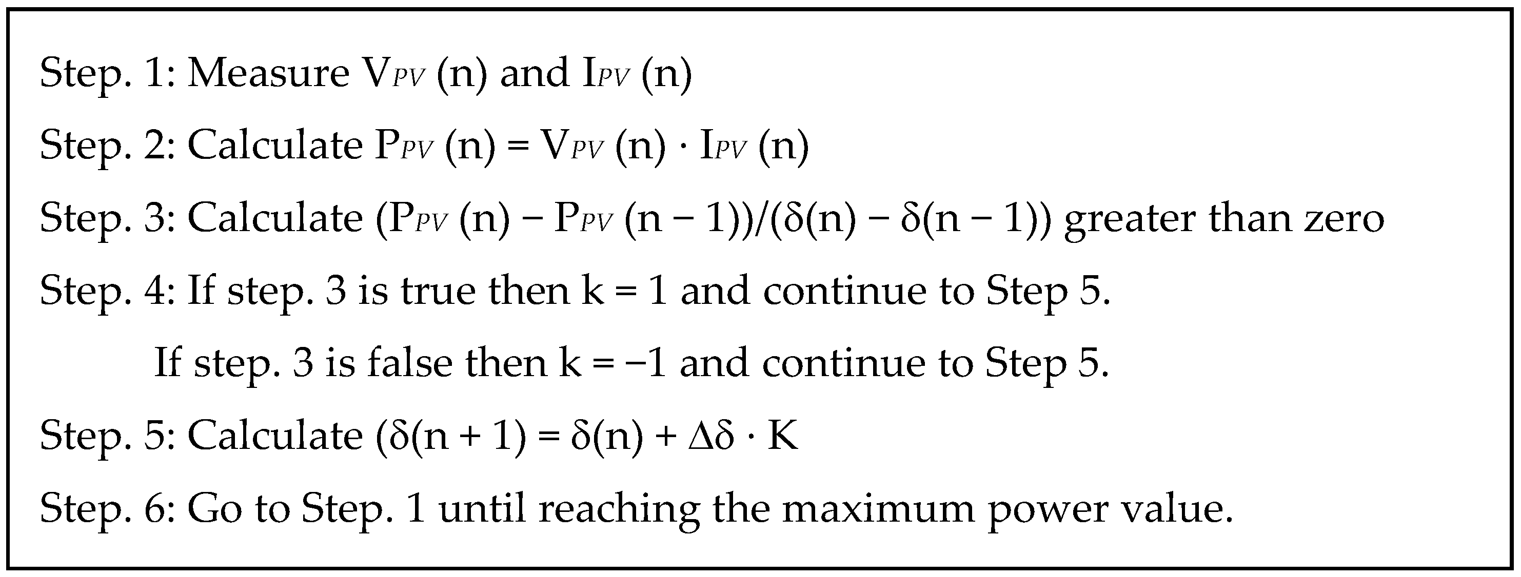
3.5. Practical Swarm Optimisation for MPPT

The proposed PSO-based MPPT algorithm’s flowchart is demonstrated in Figure 10, with the main blocks of this algorithm being outlined as follows [42,44]:

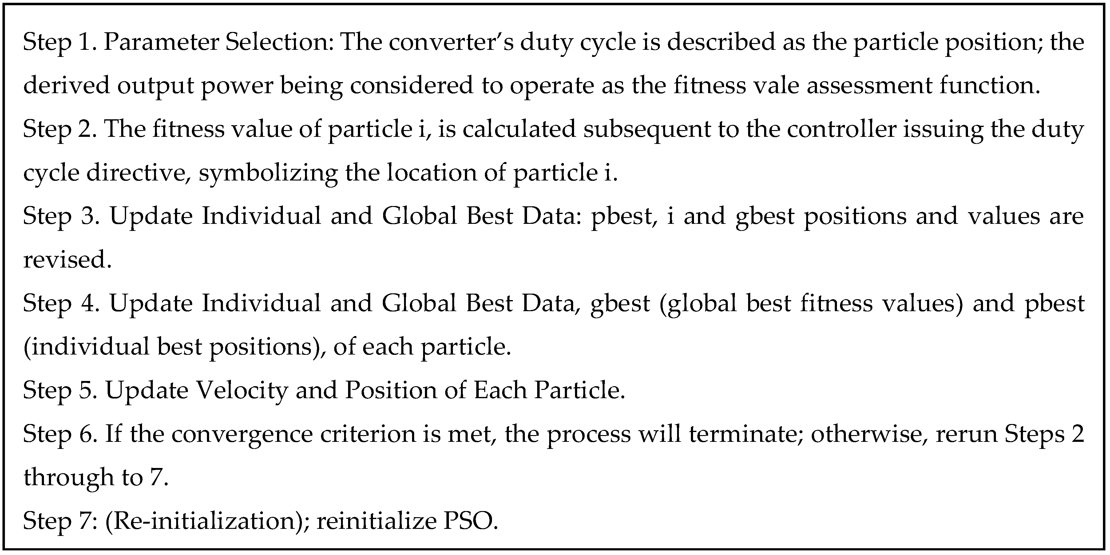
• Step 1. (Parameter Selection): As far as the planned MPPT algorithm is concerned, the converter’s duty cycle is described as the particle position; the derived output power being considered to operate as the fitness vale assessment function; with each particle’s initial 99 velocity and position being initialized at random and in a consistent distribution within the search space.
• Step 2. (Fitness Evaluation): The fitness value of particle i, is calculated subsequent to the controller issuing the duty cycle directive, symbolizing the location of particle i.
• Step 3. (Update Individual and Global Best Data): pbest, i and gbest positions and values are revised by evaluating the freshly computed fitness values with those obtained previously, plus having pbest, i, and gbest and their resultant positions replaced accordingly.
• Step 4. (Update Individual and Global Best Data): Updating fitness values, gbest (global best fitness values) and pbest (individual best positions), of each particle is achieved by having the fresh computed fitness values with the preceding examples as well as substituting the gbest and pbest equivalent to their positions as needed.
• Step 5. (Update Velocity and Position of Each Particle): By engaging the assessment of all particles, each particle’s positions and velocities in the swarm are updated via engaging PSO equations.
• Step 6. (Convergence Determination): The converge criterion are located either to the optimal solution or reach the maximum number of iterations. If the convergence criterion is met, the process will terminate; otherwise, rerun Steps 2 through to 7.
• Step 7: (Re-initialization): By considering the PSO technique, the convergence technique is either to establish the most favorable solution, or attain the maximum number of iterations. However, the fitness value in PV systems does not remain constant, since it varies respective of the applied load as well as the atmospheric conditions. For that reason, there is the need to reinitialize PSO while a search recommenced for a novel method of identifying the novel MPP upon having the output of the PV module varied.

3.6. PV Simulink Model

Figure 11 is the Simulink representation of the PV system with the DC-DC boost converter and the IC MPPT. The IC MPPT are replaced with the P&O and the PSO for comparison purposes. The system is designed to feed a DC load of 1kW and fixed AC load of 8 kW, 500 kVAR load as a small area that can be powered from the proposed standalone DC microgrid without depending on the main grid connections.

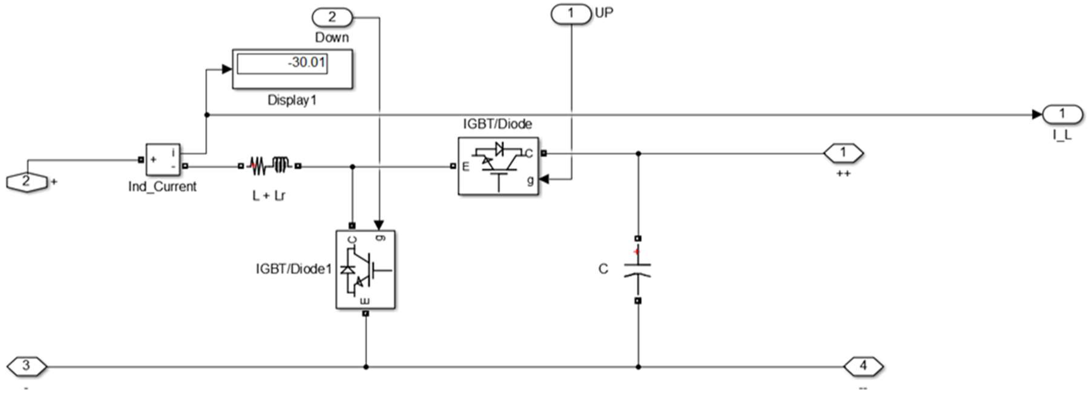
3.7. Modeling of Bidirectional Buck-boost Converter

The DC-DC buck and boost converters don’t have bidirectional power stream capacity (Figure 12). This limitation is due to the existence of diodes in the structure that stop opposite current flow [11]. Generally, a unidirectional DC-DC converter could be transformed into a bidirectional converter by supplanting the diodes with a governable switch in its construction.

Selection of inductor and capacitor: The overall converter operation depends on the design of the inductor. The primary concern is the size and weight of a powerful inductor, to the point that is may be the single heaviest part in the whole converter. To decrease the inductor weight and size, it is necessary to take a small inductance value [12]. The least inductance value expected to guarantee the converter works in continuous conduction mode (CCM) is recognized as critical inductance (LCR) value. For the buck and boost converter, the critical inductance value is reliant on the steady-state duty cycle (D), switching period (T_S) and load resistance (R_L). The critical inductance for the boost converter is:

$$L_{cr,boost}=\frac{T_S{R}_L}{2}{\left(1-D\right)}^2$$

(3)

The critical inductance for the buck mode converter is:

$$L_{cr,buck}=\frac{\left(1-D\right)T_S{V}_0}{2I_0}$$

(4)

Additionally, the input capacitor, as well as output capacitor magnitude can be found from the capacitors ripple voltage,

$$C_{in}=\frac{\Delta I_L}{8\Delta V_{in}}{T}_S$$

(5)

$$C_{out}= \frac{V_{o}D}{\Delta V_o{R}_L}{T}_S$$

(6)

where output ripple voltage is ∆V_o, inductor ripple current is ∆I_L.

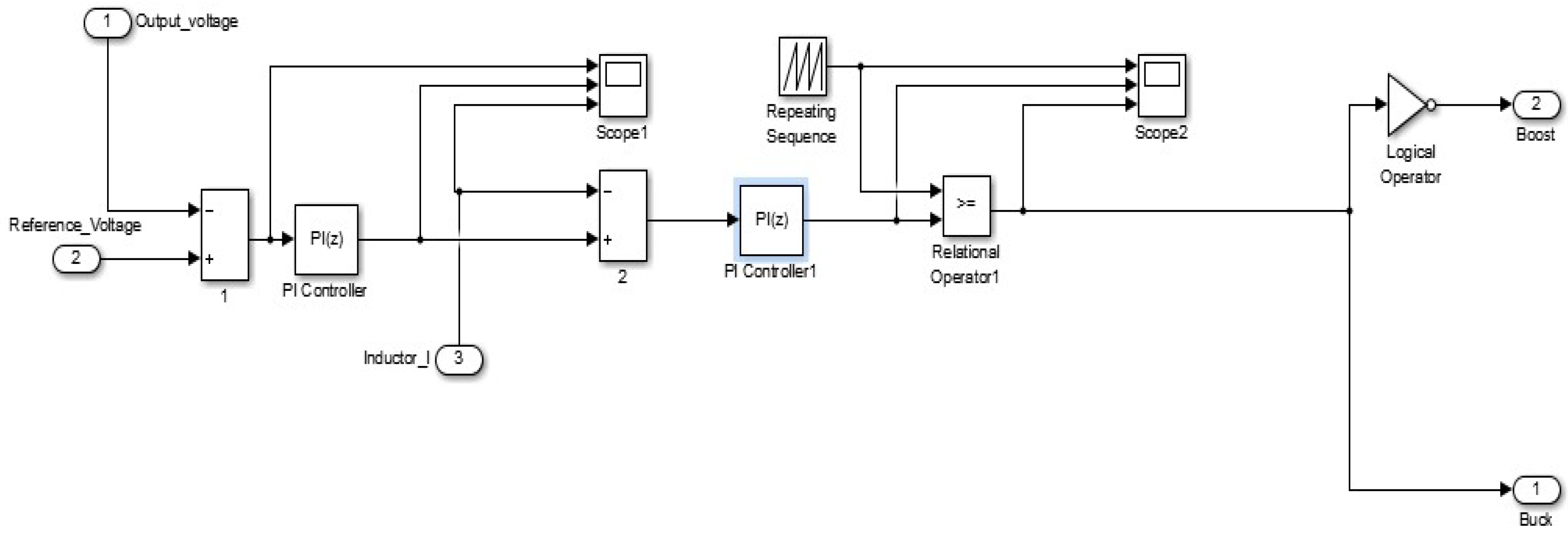
3.8. Bidirectional Buck-Boost Converter Controller

The DC voltage is controlled by changing the duty cycle in the bi-directional converter working in CCM mode. This controller keeps up a steady voltage at yield side for both boost and buck operation. The duty cycle of both switches creates by the controller. Two nested loops with the PI controller form this controller. Output voltage and inductor current are feedback signals to the PI controller (Figure 13).

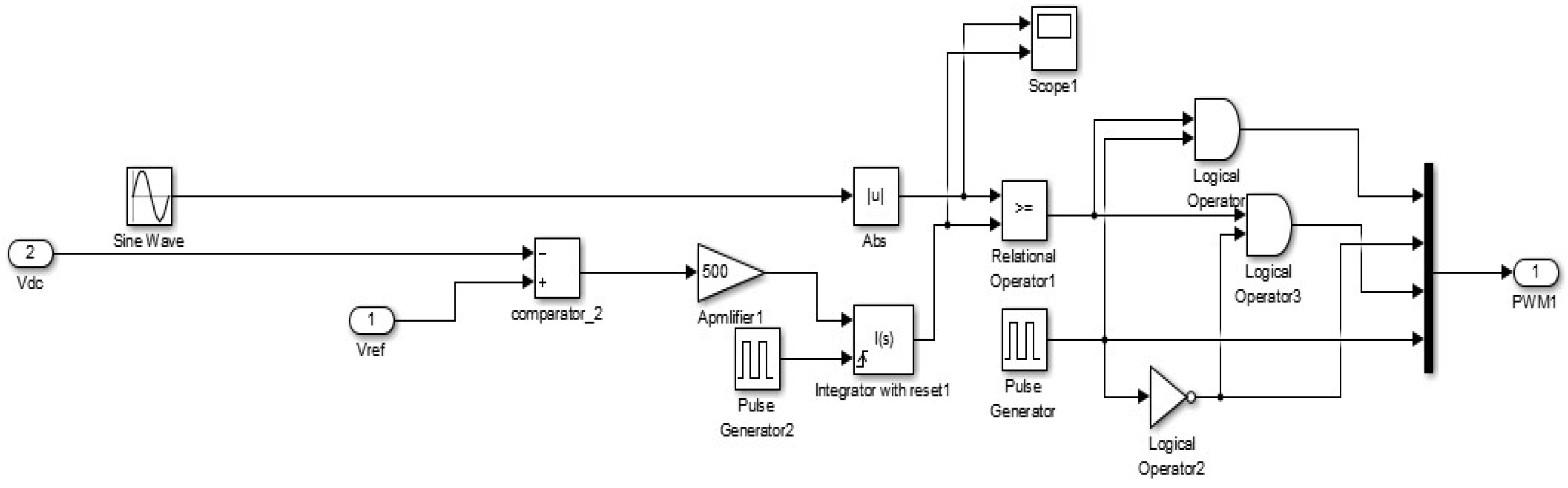
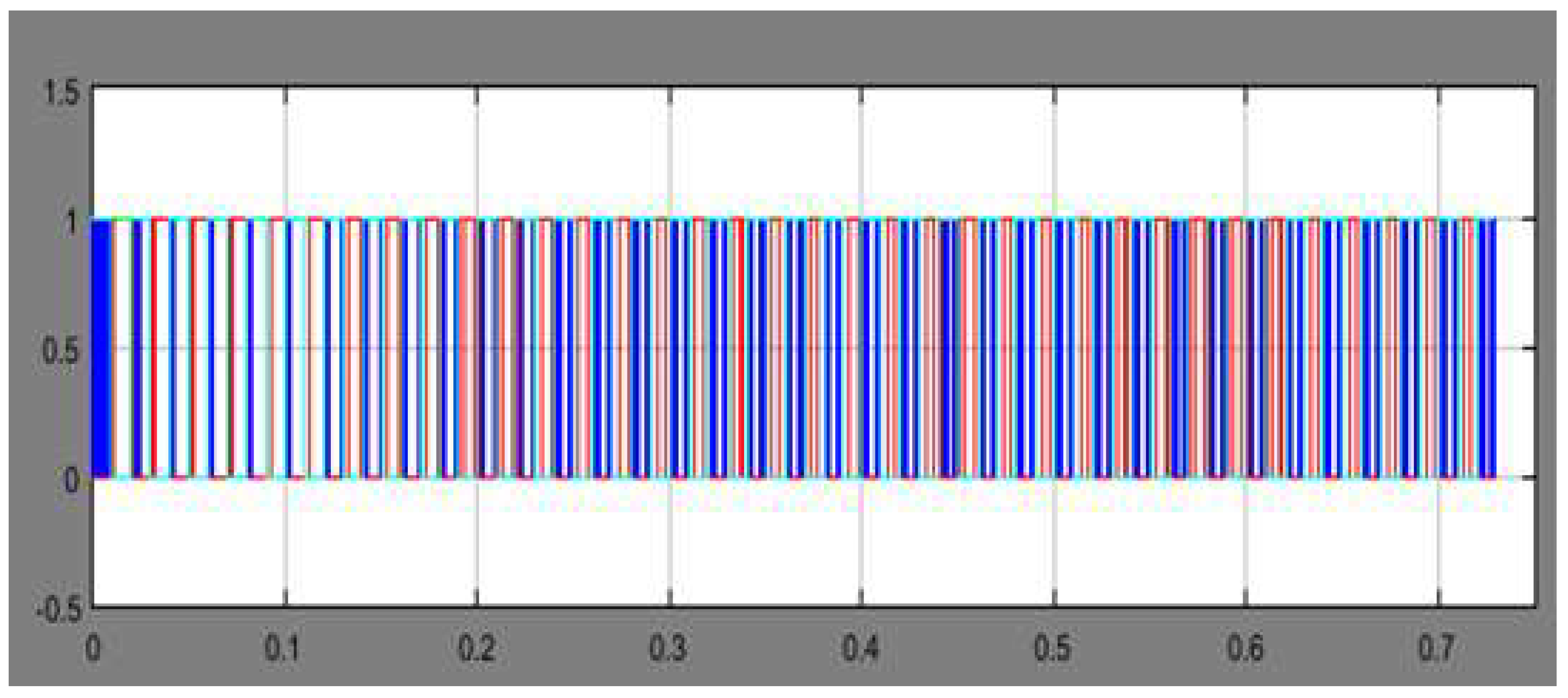
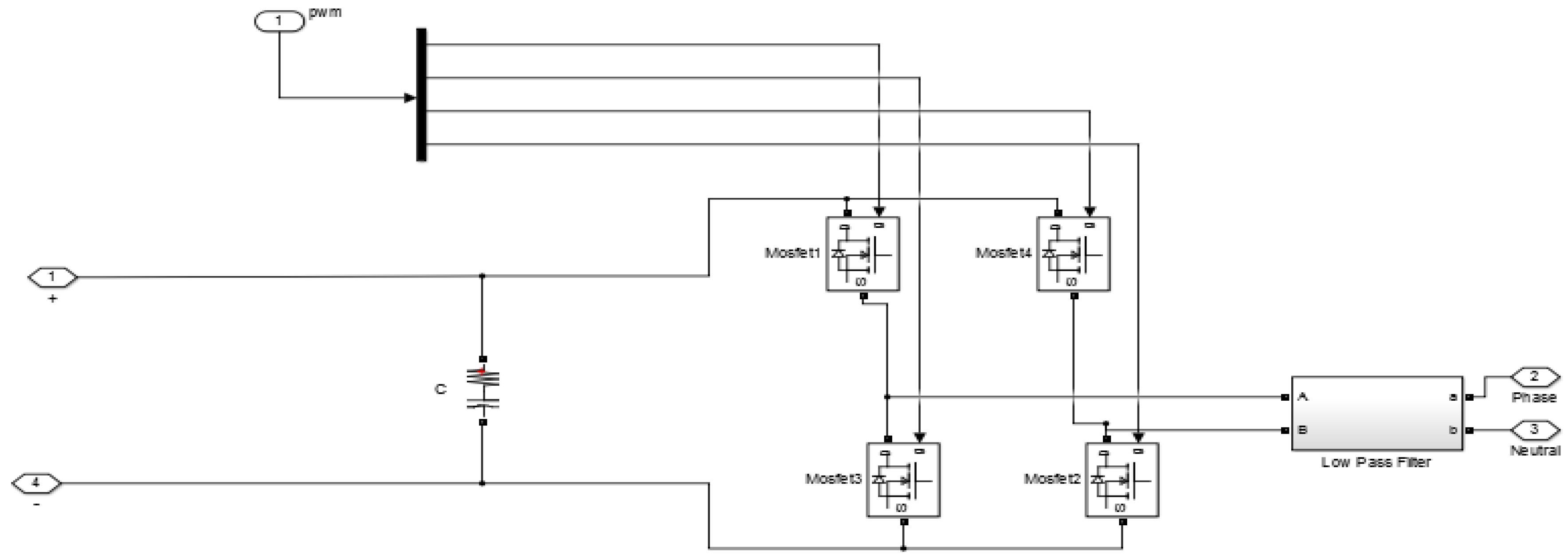
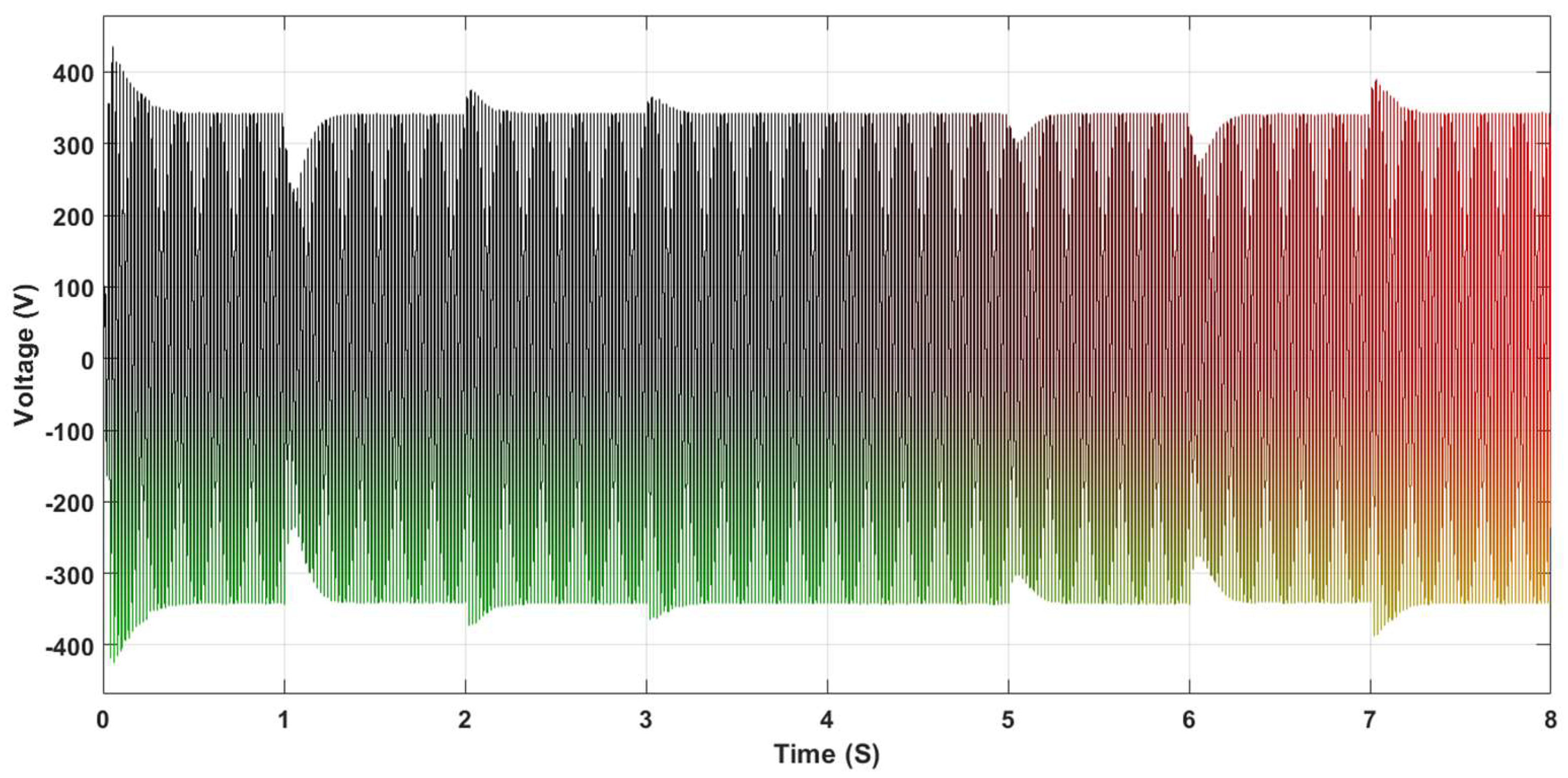
3.9. Modeling of the Inverter and Inverter Controller

An inverter consists of analog circuitry, a MOSFET driven incorporated circuit and a low-pass filter. The control circuit is involved in three fundamental blocks, the reference voltage, sine wave generator, and carrier wave generator (carrier waves can be either saw-tooth signals or triangular). At the point when these blocks are executed with comparators and other small simple circuitry, they control the PWM (Pulse-Width-Modulation) signals. The PWM signals are fed to the MOSFET drivers that perform level interpretation to drive four MOSFETs in an H-Bridge design. From here the signal is sent through a low-pass LC filter with the goal that the yield conveys a pure sine wave.

Figure 14 shows the inverter controller design to control the SPWM (Sinusoidal-Pulse-Width-Modulation) signal. Figure 15 demonstrates the signals that are passed into a comparator to achieve the PWM waveform. Figure 16 shows the generated PWM signal. Producing a sine wave adjusted on zero volts needs a negative and positive voltage across the load, for the negative and positive parts of the wave, correspondingly. This can only be accomplished from a source using four MOSFET switches organized in an H-Bridge setup. An H-Bridge converter is a switching design made out of four switches in a plan that looks like an H. By controlling distinctive switches in the bridge, a positive, negative, or zero potential voltage can be put over a load. To get a pure sine wave, the signal has been sent through a low pass filter.

In Figure 17, the design of the inverter has been shown, and the parameters used in the inverter are given in

Table 1. Inverter parameters used in the simulation.

Parameters of the Inverter	Value
Dc grid Voltage	340 VDC
DC bus capacitor	1000 µF
Filter capacitors	1000 µF
Filter Inductor	18 mH
Frequency	50 Hz

.

In Figure 17, the design of the inverter has been shown, and the parameters used in the inverter are given in Table 1.

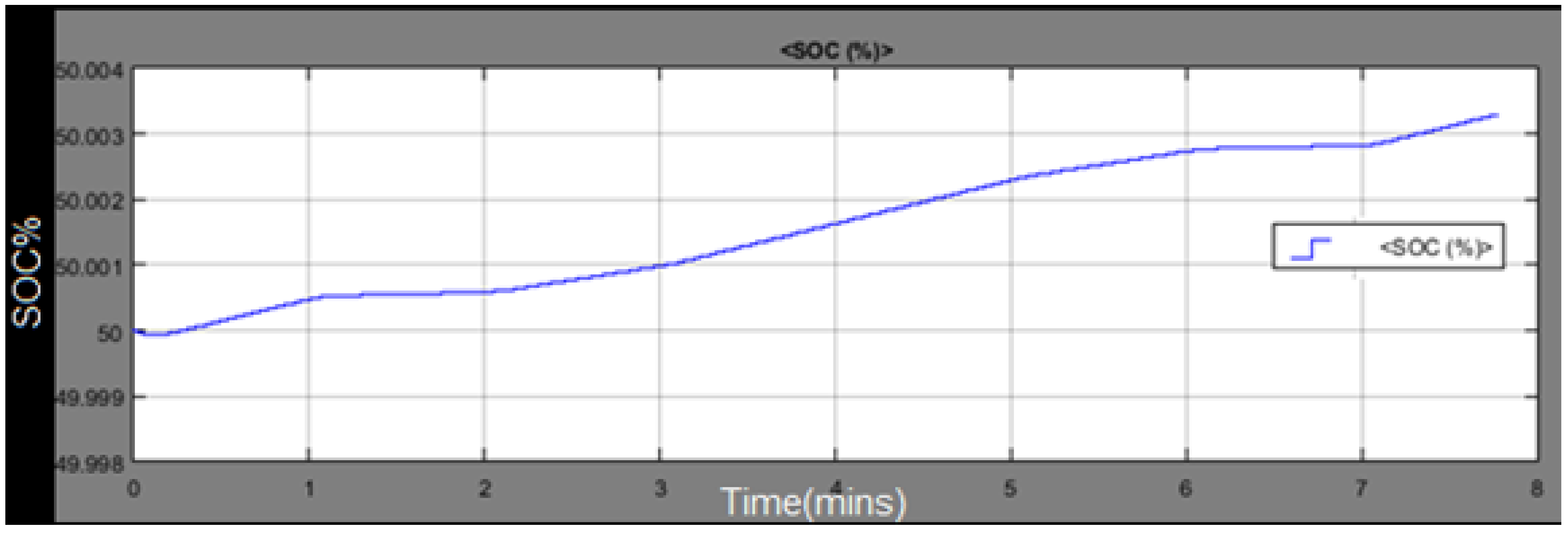
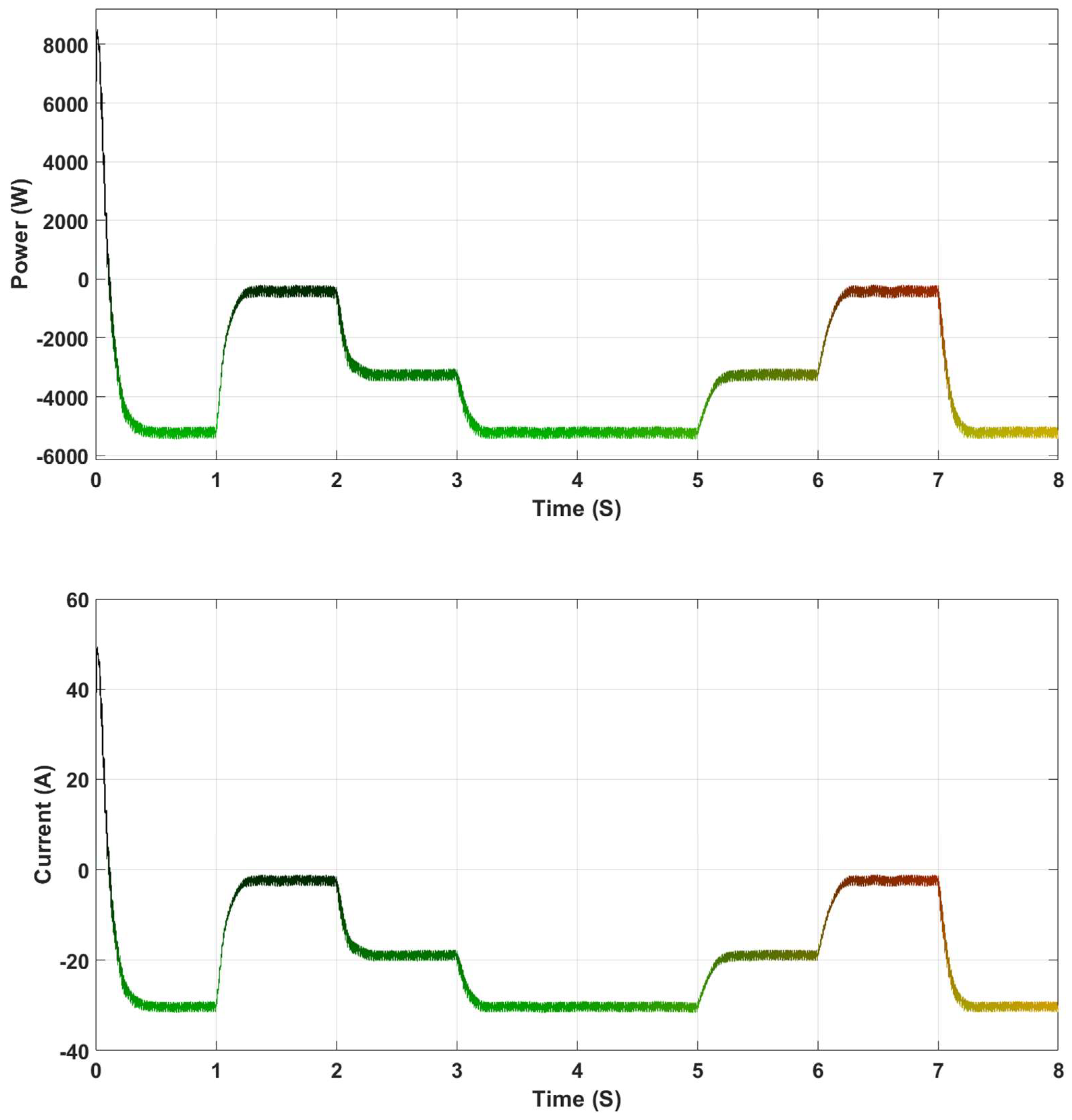
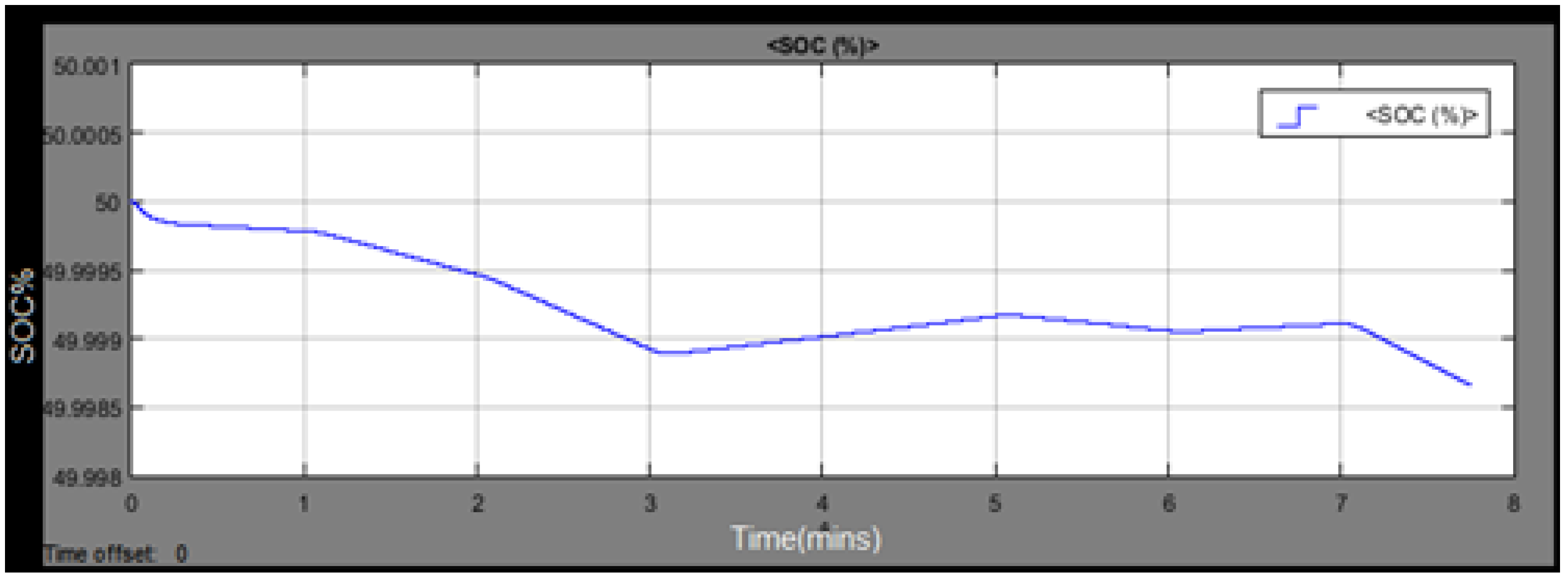
3.10. Modeling of the Battery

The battery terminal voltage V_b and state of charge (SOC) are two significant parameters for the suggestion of the battery status [13]. The battery model is given in MATLAB/Simulink. The parameters of the nickel metal hydride compose battery model are given as in

Table 2. Battery parameters used in simulation.

Symbols	Description	Value	Unit
Q	Rated Capacity	1150	Ah
SOC	Initial State-of-Charge	50	%
V	Nominal Voltage	160	V

.

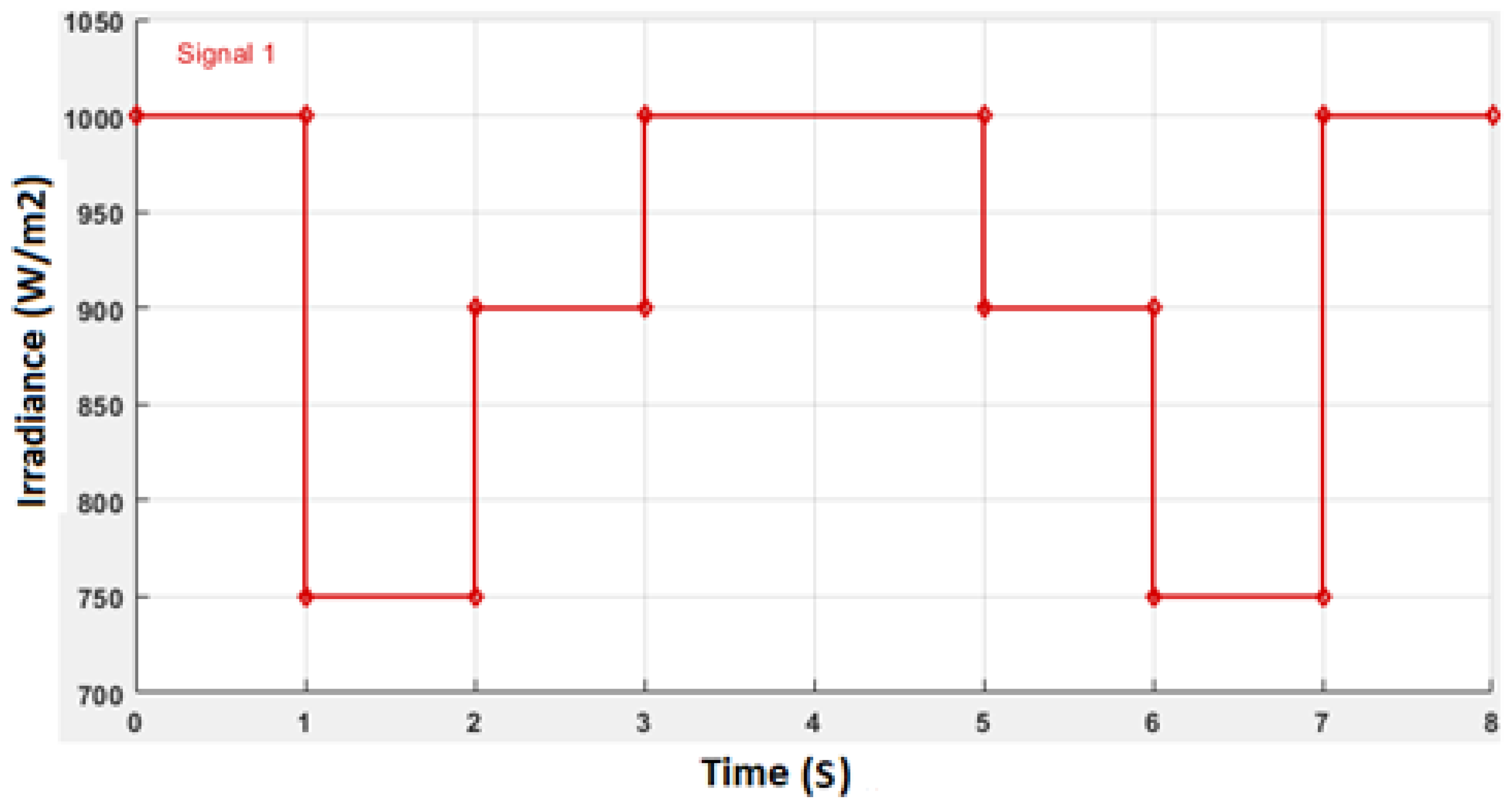
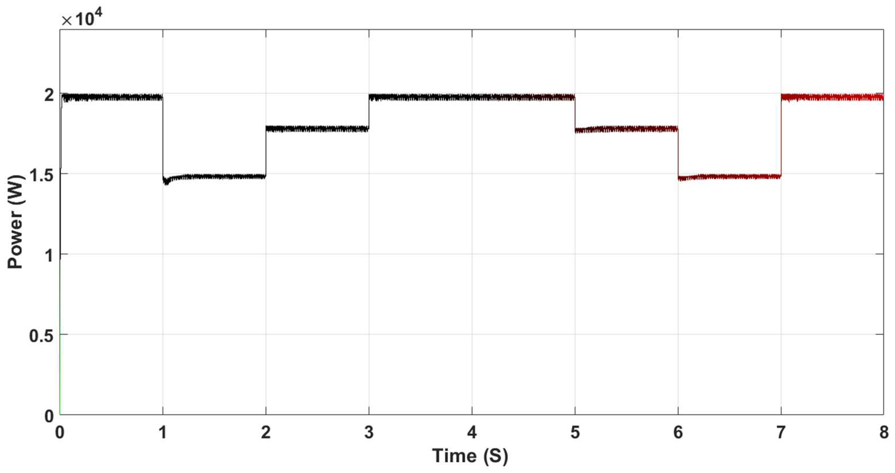
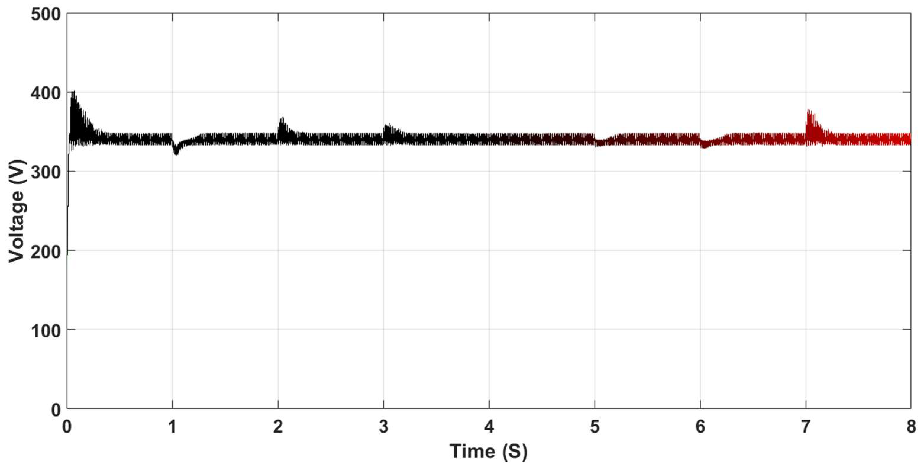
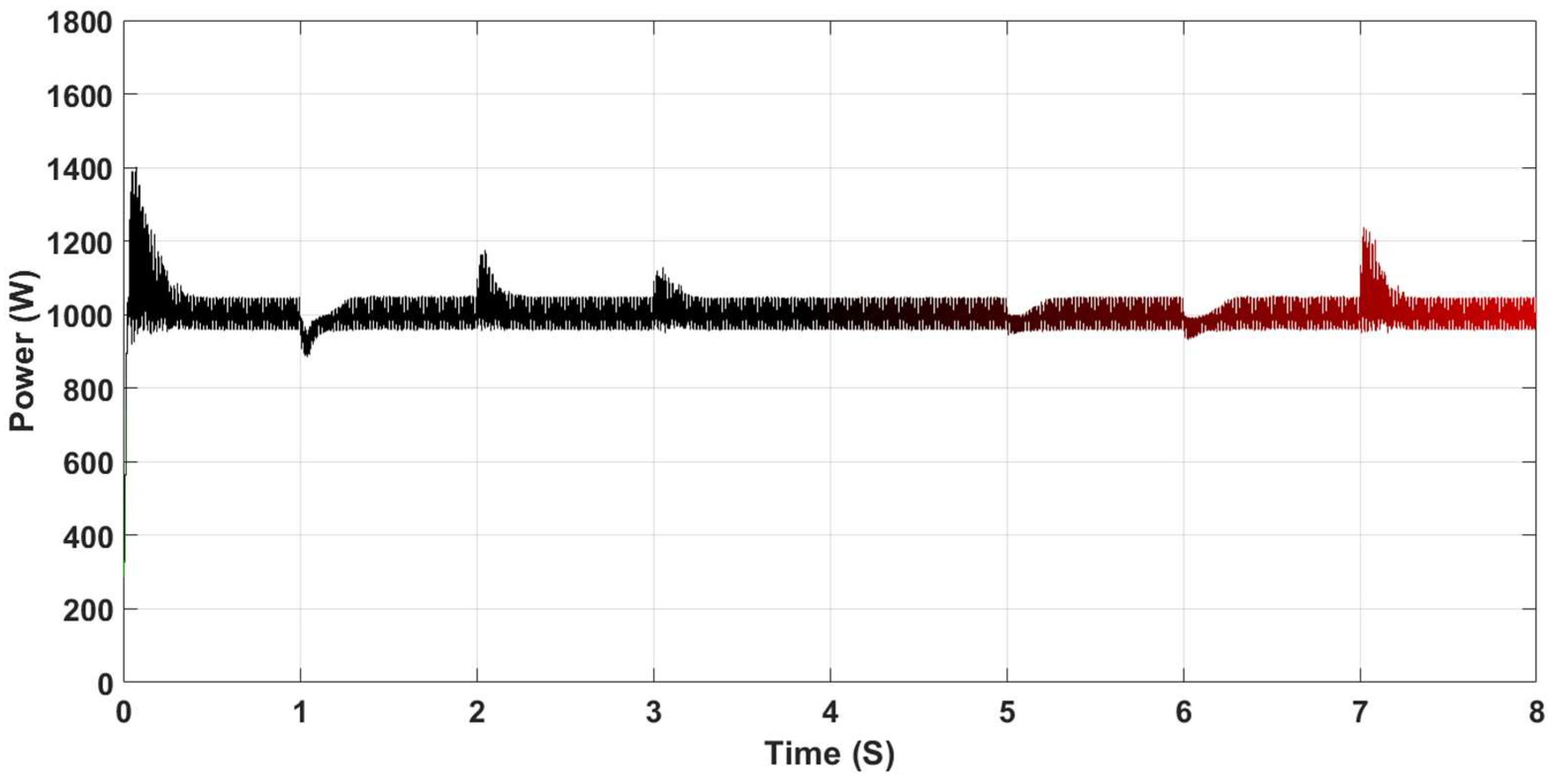
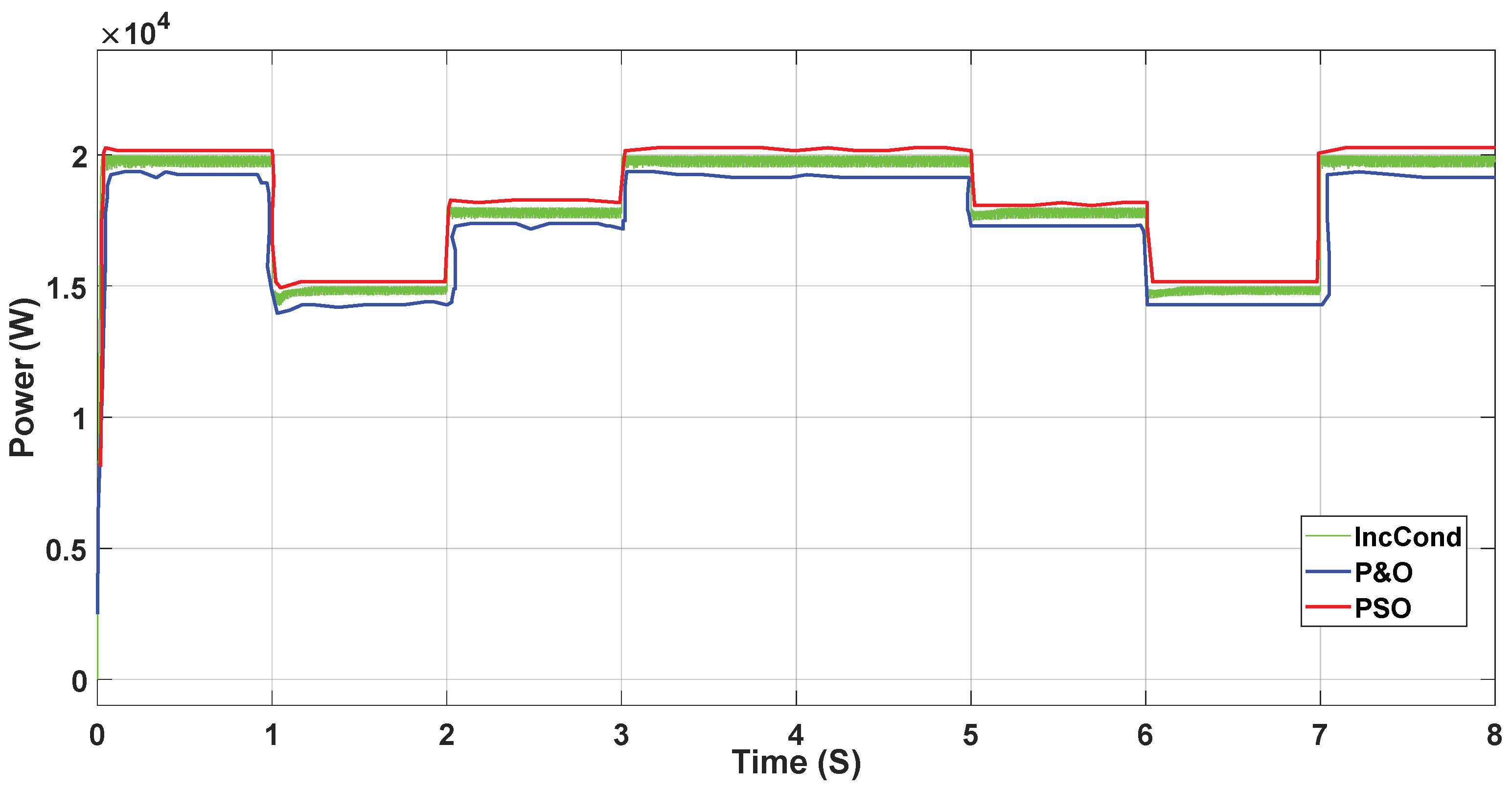
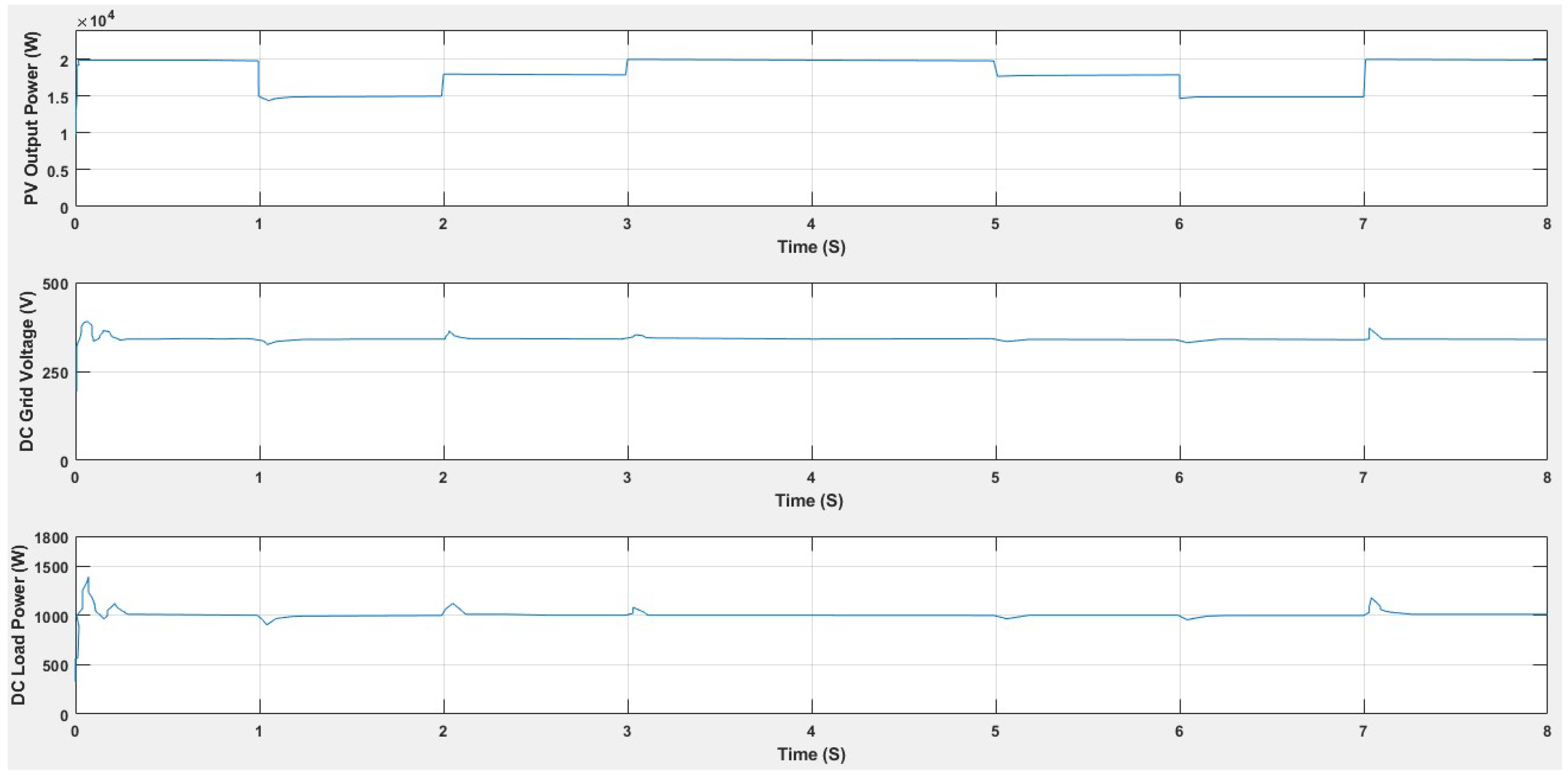
4. Input Irradiance Variation Effect

The PV array is provided with the temperature and irradiation data using a signal builder block in the Simulink. A PV array of 20 kW, IC MPPT has been used to track the highest power from the PV array, and a boost converter has been used to boost the voltage of the PV panel to its DC grid voltage of 340 V. A bidirectional buck-boost converter has been implied to control the battery charging and discharge. A fixed DC load of 1 kW and fixed AC load of 8 kW, 500 kVAR load, have been fed from this system. As this system is producing DC voltage, a DC to AC inverter is implied to power the AC loads of this system. Figure 18 shows the input irradiance for the system, and we consider an ambient temperature of 25 °C for this simulation. In this figure, different irradiance levels are proposed with respect to the time as happens in real life. Then, different MPPT techniques are investigated with the aid of real-time simulator to check the fast-dynamic response.

In Figure 19 the power produced by the solar PV panel are variable in terms of time depending on the solar irradiation. When the irradiance is 1000 W/m², the PV gives the highest power similar to its rating at almost 20 kW. While decreasing the irradiance, the power output of the PV also decreases with time. As described above, in this system the DC grid voltage of 340 V has been used. DC grid voltage and power supplied to DC load obtained in simulation as shown in Figure 20. As the PV array cannot produce less than the grid voltage, the DC-DC boost converter boosts the PV array voltage to 340 V. From the figure, we can see that DC grid voltage is around 340 V and the power supplied to the DC load is around 1000 W though there are fluctuations when the irradiance suddenly drops down or goes up for both the DC grid voltage and power provided to the DC load.

The PV system supplies DC power, and to supply the power to the AC loads, a DC-AC inverter is used. Figure 21 shows the AC voltage across the AC load, where there is also the sudden decrease and increase of voltage due to the sudden decline and rise of the irradiance.

One of the main components of the system is the bi-directional buck/boost converter. The common DC link voltage (DC grid) is kept constant by the bi-directional flow of power between the battery and PV system. If the voltage increases above the predefined grid voltage value, i.e. 340 V that means the PV system power is enough to feed the load and charge the battery and therefore, some current is sent to the battery to take the voltage down to 340 V, and in this case the bidirectional converter is operated in buck mode, stepping down the voltage from 340 V to 160 V (Battery Voltage). If the DC grid voltage goes down below 340 V, this means the PV is not producing enough power to feed the load and therefore, some current is sent from the battery to the grid and in this case, the battery discharges and the bidirectional converter is operated in boost mode, i.e., boosting the voltage from 160 to 340 V. Initially, the battery state of charge (SOC) is selected as 50%. With the input irradiance in Figure 18, the battery is in charging mode as the PV system is producing enough power to feed the loads as well as charge the battery, so the battery SOC is increasing at the time, as shown in Figure 22. The bidirectional buck-boost converter is working in buck mode, the DC input voltage 340 V is buck to 160 V by controller pulses.

As the battery is charged and the bidirectional buck-boost converter is in buck mode, the battery current and power is negative, as shown in Figure 23.

While giving the input irradiance bellow 700 W/m², the produced power from the PV system is not enough to feed the loads, so the bidirectional converter is working in boost mode to make the battery voltage from 160 V to 340 V, causing the battery to discharge as shown in the Figure 24. When the input irradiance is more than 700 W/m² the battery works in charging mode, as in the 3 and 4 mins the irradiance is around 790 W/m² and the battery charges during this period.

OPAL-RT real-time simulator (Hardware-in the-loop) is a platform set of test application on the basis of modeling and has the ability to conduct hardware within the loop and rapid control prototyping. The type of the user equipment is OP4510 RT-LAB-RCP/HIL, which is located in the authors’ research lab [42] and is shown in Figure 25 and it is manufactured by Canadian company with the name OPAL. Hardware-in-the-loop (HIL) simulation is a well-established prototyping approach that aims to reduce design costs of power systems by running comprehensive tests early in the development phase. Real-time simulation refers to a computer model of a physical system that can execute at the same rate as actual "wall clock" time. In other words, the computer model runs at the same rate as the actual physical system.

It employs a special technique to integrate a complicated model into multiple subsystems, which will operate simultaneously. The OP4510 is a compact device with 128 fast I/O channels with signal conditioning, additional RS422 channels (or optional low-speed fiber optic channels), high-speed communication ports (SFPs), and is fully integrated with Simulink, Sim-Power-System. The integration of high-end INTEL multi-core processors with powerful Kintex 7 FPGA (Field-Programmable-Gate-Array) provides greater simulation power and sub-microsecond simulation time steps to maximize the accuracy of fast power electronic systems. A programmable FPGA is installed within the target machine and 10 ns is the frequency of the digital I/O channel, pulse resolution. One simulation step can obtain or generate multiple pulse events in the platform of the RT-LAB simulation system. In this way, the IGBT (Insulated-Gate-Bipolar-Transistor) switch in the electric inverter can be provided with highly précised timing. If the events of FPGA can be combined by identifying the unique real-time algorithm and function of RE-EVENTs, then 10μs can be obtained as the simulation step [40,41,42].

The models that are installed by Simulink are to be compacted out of the apex and the OPAL-RT library’ parameters such as SM, SS, and SC should be used to name the RT-LAB so that functions of various parts can be ensured. Curve within the simulation system, data communication among the main parameters, and real-time observation are performed by the SC subsystem. Data are gathered and displayed with the help of a fundamental module found in the programs. The SM subsystem takes over the responsibility of network synchronization and real-time observation. The SS subsystem normally belongs to the system models involved in the simulation. The segregated model comprises one SM subsystem, one SC subsystem, and SS subsystem. There are only switch, oscilloscope, and logic selection and no calculating parts in the SC subsystem. The Opcomm synchronous communication module holds a significant part in simulation, and each signal has to reach the subsystem above via undergoing the Opcomm module [40,41,42].

Figure 26 demonstrates testing main program with 10 μs as the simulation step. The SM subsystem has the tenacity of completing the simulation calculation along with the synchronous communication of the MPPT. The improved incremental conductance technique is implemented in the experimentation. The module’s vulnerable to the events are replaced by RT-EVENTS (Real-Time events to transform the module from Simulink into real-time) modules. PWM signal is giving accurate output. The digital output module of RT-LAB is the OP5110-5120 Digital Out that has the ability to carry out the output of the PWM signal. The analog input module is the Analog in that, also has the ability to carry out the input of current and voltage of the photovoltaic cell. FPGA has been blended with the synchronous drive module that is the OP5110- 5120 Opsync. The SC subsystem has the ability to perform current, system information, voltage, and power of the photovoltaic cell. Due to the same sampling rate of four signals, only one Opcomm module is required.

Figure 27 shows samples of the output testing data from the OPAL-RT real-time simulator (HIL). The comparison between these samples for PV output power, DC grid voltage, and DC load power from the real-time simulator with the previous results from the Simulink model shows a great matching of the same results with a minimal error under variable irradiance values.

The proposed three techniques are compared for validity purposes to show the best dynamic response and best MPP value under different levels of irradiance from Figure 18. Figure 28 shows the highest obtained maximum power is achieved from the particle swarm optimization (PSO) with a good dynamic response too. However, the incremental conductance (IncCond) MPPT is better than perturb and observe (P&O) choice in both fast—dynamic response and MPP value.

Figure 29 displays a comparison between PSO, P&O, and IncCond MPPTs at 1kW irradiance and 25 °C. It shows the difference in the fast—dynamic response for the three techniques with the PSO MPPT as the first ranked one in MPP value and it reaches its MPP faster. The second-ranked one is the IncCond MPPT which is very close to the PSO one with little-bit harmonics. However, the P&O MPPT is the lowest one in terms of MPP and dynamic response with more harmonics or oscillations, especially at the beginning.

5. Stability Analysis Investigation

It is very important to perform the steady-state and transient stability analysis on both the AC and DC microgrid to ensure good quality and constant power supply. The DC microgrid has faster stability incomparable with the AC microgrid after the fault clearance without any effect when it is connected to a weak grid. The microgrid and the traditional power system stability have the same basic concepts. However, because of the presence of the high-level-penetration of DG sources with their associated converters, the microgrid stability glitches are originated or heavily affected by the converters’ dynamics and control. There are different techniques to examine and predict the stability of microgrids to provide systematic tools for microgrid controllers design. A mixture of a small-signal and time-domain simulation is usually used for inclusive stability analysis.

Stability analysis of the microgrid has significant effect with the increase of intermittent renewable energy sources penetration. The proposed stability analysis investigation is using a logic of global/semi-global stability [45,46,47], rather than using prevailing small-signal-analysis methods. The present tactics to stability analysis are mainly based on time-domain, energy function, and Lyapunov-function. This work shapes a simple stability analysis way based on the polynomial-Lyapunov-function, which is calculated algorithmically utilizing the sum-of-squares optimization to maximize the region of attraction (ROA) of an equilibrium solution. This process rules out the essential for previous information of the formula of the Lyapunov or energy function. Because of the mentioned reasons and the essential effect of the power electronics converters with their controllers on the system stability, this part proposes simple investigation for the DC-DC boost controller and bidirectional DC-DC buck-boost converter with their controllers. The DC microgrid almost doesn’t have harmonic effects, and skin effect or Ferranti effect. Because of its advantages, it may be the perfect candidate for the future power systems over the AC microgrid [7,48,49].

Another widespread analytic method for grid-connected inverters is the impedance-based stability principle. Many control techniques are proposed to improve the microgrid stability such as novel frequency regulation by using the kinetic energy from the loads or load-voltage-sensitivity and adaptively controlling converters [50,51,52,53,54]. The general microgrid stability as same as the normal power system stability definition in reference [55], which is: “The ability of an electric power system, for a given initial operating condition, to regain a state of operating equilibrium after being subjected to a physical disturbance, with most system variables bounded so that practically the entire system remains intact.” The frequency stability is “the ability of a power system to maintain steady frequency following a severe system upset resulting in a significant imbalance between generation and load. [55]” And the voltage stability refers to ”the ability of a power system to maintain the steady voltage at all buses in the system after being subjected to a disturbance from a given initial operating condition. [55]” “Similar to the bulk power system, the microgrid frequency stability largely depends on the real power demand-supply balance and the reactive power balance is critical for microgrid voltage stability [49]”. The instability of the power converter controllers can affect microgrid loss synchronism and cause prohibited complete system voltage profiles. A sustained low voltage condition can outcome due to inadequate microgrid abilities to loose regulate system voltage after the contingencies [56,57].

The polynomial Lyapunov function for stability analysis of a DC-nanogrid is investigated. The proposed method depends on semi-definite optimization with identifying the region of attraction (ROA) of the equilibrium point without the aid of time domain choice for solution [45,46,47] with power electronics converters. The dynamic modeling of the DG source is formulated and converts into state-space equations. The equilibrium solutions for all states and used Taylor series are identified. The Lyapunov function V(x) is calculated to satisfy the Lyapunov conditions in a domain Ω around the equilibrium solution (located at x = 0, where x is the state variables vector) given as follows:

$$\{\begin{array}{c}V\left(x\right)>0 for \forall x\ne 0\\ V\left(0\right)=0\end{array}$$

(7)

$$\dot{V}\left(x\right)=\nabla V\left(x\right)·F\left(x\right)\le 0for\forall x$$

(8)

$$\dot{x}=F\left(x\right);\left(x\right):\mathrm{The}\mathrm{functions}\mathrm{of}\mathrm{the}\mathrm{system}\mathrm{differential}\mathrm{equations}$$

(9)

$$V(x)<\gamma ,\forall x\in ROA$$

(10)

After that, we determine the Lyapunov function (LF) and assess system state x stability by checking the condition V(x) < γ. Then, we determine feasibility of the sum of squares (SOS) for optimization in order to identify a Lyapunov polynomial function and identify the ROA estimate of the equilibrium.

Illustration of system stability using Lyapunov function (Equations (7)–(10)) for best estimation of ROA is presented. The optimization technique will help find best LF with the widest estimate of ROA. A set inclusion problem is formulated to make V(x) satisfying the Lyapunov conditions in the widest possible domain, as shown in the following:

• Set A: Set of the states x within an arbitrary “radius” $\beta$ (in other word, satisfying the inequality p(x) < β, where p(x) has an arbitrary shape)
• Set B: Set of the states x for which an arbitrary $\gamma$ is an upper bound of the Lyapunov function V(x);
• Set C: Set of the states x for which $\dot{V}\left(x\right)$ is negative. It should be noted that this the only set that depends directly on F(x);

$$\begin{array}{c}\mathrm{Set}\mathrm{A}\subseteq \mathrm{Set}\mathrm{B}\subseteq \mathrm{Set}\mathrm{C}\\ \mathrm{Max}\beta ,\gamma \mathrm{subject}\mathrm{to}\mathrm{Set}\mathrm{A}\subseteq \mathrm{Set}\mathrm{B}\subseteq \mathrm{Set}\mathrm{C}\end{array}$$

(11)

$$\begin{array}{c}{S}_1=\left\{x\in R^n:g_1\left(x\right)\le 0\right\}\\ S_2=\left\{x\in R^n:g_2\left(x\right)\le 0\right\}\end{array}$$

(12)

$$\begin{array}{c}-g_1\left(x\right)+\lambda \left(x\right)·g_2\left(x\right)\\ \mathrm{Max}\beta ,\gamma \text{ subject to}\end{array}$$

(13)

$$V\left(x\right)-L_1\left(x\right)\mathrm{is}\mathrm{SOS}$$

(14)

$$-\left[\nabla V\left(x\right)·F\left(x\right)+L_2\left(x\right)+s_2\left(x\right)·\left(\gamma -V\left(x\right)\right)\right]\mathrm{is}\mathrm{SOS}$$

(15)

$$-\left[\left(V\left(x\right)-\gamma \right)+s_1\left(x\right)·\left(\beta -p\left(x\right)\right)\right]\mathrm{is}\mathrm{SOS}$$

(16)

$$L_1\left(x\right)={\in }_1{x}^{T}x,L_2\left(x\right)={\in }_2{x}^{T}x$$

(17)

Stability analysis steps [47]:

• Step 1: “To start the VS iteration, a first estimation of the LF is determined using the linear approximation of (3) in the vicinity of the equilibrium point yielding the following”;

  $$\dot{x}=A·x$$

  (18)

  where “A is the Jacobian of F(x). Once A has been determined, if all of its eigenvalues are found to have negative real parts, then there exists a positive-definite matrix P (where Q must be positive definite) that satisfies the following condition”

  $$A^{T}P+PA+Q=0$$

  (19)
  The corresponding LF is determined using:

  $$V=x^{T}Px$$

  (20)
• Step 2: “In this step, V(x) is held fixed while $\gamma$ and $s_2\left(x\right)$ are determined using Equations (15) and (17), using the bisection method to iteratively determine the biggest value of $\gamma$;”
• Step 3: “In this step, V(x) is held fixed while both $\beta$ and $s_1\left(x\right)$ are determined using Equation (16). However, Equation (10) is bilinear in $\beta$ and $s_1\left(x\right)$, bisection is used to obtain $s_1\left(x\right)$ while keeping $\beta$ fixed”
• Step 4: “In this step $\beta$, $\gamma$, $s_1\left(x\right)$, and $s_2\left(x\right)$ are held fixed while V(x) is determined using Equations (14) through (17) and normalized with respect to $\gamma$ to avoid numerical problem”;
• Step 5a: “If the value of $\beta$ converges, the iteration process is stopped; otherwise, the process flow restarts at step 2”;
• Step 5b: “Determine the variation in the shaping function following”

  $$\Delta p\left(x\right)=p\left(x\right)-V\left(x\right)$$

  (21)

To carry out the previous portion of the work, we use software SOSTOOLS 2.05, SeDuMi 1.3, and Multipoly 2.00.

For the stability analysis of the proposed system in previous section the two controllers, DC-DC boost controller and bidirectional DC-DC buck-boost converter are considered (Figure 30).

We consider two controls in the model. The control signals are duty cycles of the converters. S1 controls the power output of the PV; S2 controls the DC bus voltage. Utilizing Kirchhoff’s laws, the dynamic model of the system can be composed as:

$$L_1\frac{d{i}_1}{dt}=v_1-v_2\left(1-s_1\right)$$

(22)

$$C_1\frac{d{v}_1}{dt}=i_D-i_1=I_{ph}-I_0\left(e^{av1}-1\right)-\frac{v_1}{R_p}-i_1$$

(23)

$$L_2\frac{d{i}_2}{dt}=E-i_{2}r-v_2{s}_2$$

(24)

$$C_2\frac{d{v}_2}{dt}=i_1\left(1-s_1\right)+i_2{s}_2-\frac{v_2}{R_1}$$

(25)

with the constraints: v₂ > 0, i₁ > 0.

Let x_T = [x₁, x₂, x₃, x₄] = [i₁, v₁, i₂, v₂] and the system can be rewritten as state space model:

$$\dot{x_1}=\frac{1}{L_1}\left[x_2-x_4\left(1-s_1\right)\right]$$

(26)

$$\dot{x_2}=\frac{1}{C_1}\left[I_{ph}-I_0\left(e^{ax2}-1\right)-\frac{x_2}{R_p}-x_1\right]$$

(27)

$$\dot{x_3}=\frac{1}{L_2}\left[E-r{x}_3-x_4{s}_2\right]$$

(28)

$$\dot{x_4}=\frac{1}{C_2}\left[-\frac{x_4}{R_1}+x_1\left(1-s_1\right)+x_3{s}_2\right]$$

(29)

with the constraints: x₁ > 0, x₄ > 0

Moving the equilibrium points of the system to the origin and the system without control which is s = 0 is globally asymptotically stable [17].

$$f\left(x,0\right)=\left|\begin{array}{c}\frac{1}{L_1}\left[x_2-x_4\right]\\ \frac{1}{C_1}\left[-x_1-\frac{x_2}{R_p}-I_0{e}^{a{x}_2}\left(e^{a{x}_2}-1\right)\right]\\ \frac{1}{L_2} \left[-r{x}_3-x_4\right]\\ \frac{1}{C_2}\left[x_1-\frac{x_4}{R_1}\right]\end{array}\right|$$

(30)

with the Lyapunov function:

$$V\left(x\right)=\frac{1}{2}{L}_1{x}_1^2+\frac{1}{2}{C}_1{x}_2^2+\frac{1}{2}{L}_2{x}_3^2+\frac{1}{2}{C}_2{x}_4^2$$

(31)

$$\dot{V}\left(x\right)=L_1{x}_1{\dot{x}}_1+C_1{x}_2{\dot{x}}_2+L_2{x}_3{\dot{x}}_3+C_2{x}_4{\dot{x}}_4$$

(32)

Considering only the boost converter and replacing the values of parameters with s₁ as zero we get;

$$\dot{x_1}=20000\times \left[x_2-x_4\right]$$

(33)

$$\dot{x_2}=\frac{1}{1000\times {10}^{-6}}\left[8.5795-2.0381\times {10}^{-10}\left(e^{11622.095x2}-1\right)-\frac{x_2}{301.81}-x_1\right]$$

(34)

Computing a quadratic Lyapunov function V(x) for the system

$$V_1=0.1836\times x_1^2+1.506\mathrm{e}-18\times x_1\times x_2+0.3134\times x_2^2$$

(35)

Considering only the bidirectional buck-boost converter and replacing the values of parameters with s₂ as zero we get;

$$\dot{x_3}=\frac{1}{5\times {10}^{-5}}\left[160-0.0039\times x_3\right]$$

(36)

$$\dot{x_4}=\frac{1}{1000\times {10}^{-6}}\left[-\frac{x_4}{0.0001}\right]$$

(37)

Computing a quadratic Lyapunov function V(x) for the system

$$V_2=0.2476\times x_3^2+5.654\mathrm{e}-7\times x_3\times x_4+272.3x_4^2$$

(38)

6. Conclusions

In this paper, important aspects of the solar renewable energy source have been explored. The possibilities of the DC microgrid system and its viability have been investigated. A complete design and analysis have been proposed to effectively enhance the power conversion efficiency of a standalone solar PV system with DC microgrid. A PV array of 20 kW, IC MPPT, a boost converter, and a bidirectional buck-boost converter have been implied to control the battery charging and discharging. The proposed converter decreases the component losses and upsurges the performance of the complete system by peer selection of its components. Additionally, PSO and P&O MPPT techniques are proposed incomparable with the IncCond one. Particle Swarm Optimization (PSO) one is the best in terms of fast—dynamic responses with the fast change of irradiance with better maximum power point (MPP). The IncCond one gives very good results close to the PSO and better than the P&O. A fixed DC load of 1kW and fixed AC load of 8kW, 500kVAR load, have been fed from this system. Later, a stability analysis of the DC microgrid for the boost controller and bidirectional buck-boost controller have figured out the space state equations and Lyapunov function using sum-of-squares optimization. The proposed complete system lessens the component losses and upsurges the efficiency of the complete system in terms of enhancing the dynamic response, minimizing harmonics’ loss, and getting more stable value for the maximum power point. The Simulink system is validated utilizing OPAL-RT Hardware-In-the-Loop and shows a great matching for the results.

References

1. Haque, A.; Rahman, M.A.; Ahsan, Q. Building integrated photovoltaic system: Cost effectiveness. In Proceedings of the 2012 7th International Conference on Electrical and Computer Engineering, Dhaka, Bangladesh, 20–22 December 2012; pp. 904–907. [Google Scholar]
2. Haque, A.; Rahman, M.A. Study of a solar PV-powered mini-grid pumped hydroelectric storage & its comparison with battery storage. In Proceedings of the IEEE Electrical & Computer Engineering (ICECE) 7th International Conference, Dhaka, Bangladesh, 28–30 December 2012; pp. 626–629. [Google Scholar]
3. Li, C.; de Bosio, F.; Chaudhary, S.K.; Graells, M.; Vasquez, J.C.; Guerrero, J.M. Operation cost minimization of droop-controlled DC microgrids based on real-time pricing and optimal power flow. In Proceedings of the IECON 2015-41st Annual Conference IEEE Industrial Electronics Society, Yokohama, Japan, 9–12 November 2015; pp. 003905–003909. [Google Scholar]
4. Arifin, M.S.; Khan, M.M.S.; Haque, A. Improvement of load-margin and bus voltage of Bangladesh power system with the penetration of PV based generation. In Proceedings of the 2013 International Conference IEEE Informatics, Electronics & Vision (ICIEV), Dhaka, Bangladesh, 17–18 May 2013; pp. 1–5. [Google Scholar]
5. Islam, M.; Mekhilef, S. High efficiency transformerless MOSFET inverter for grid-tied photovoltaic system. In Proceedings of the 2014 Twenty-Ninth Annual IEEE Applied Power Electronics Conference and Exposition (APEC), Fort Worth, TX, USA, 16–20 March 2014; pp. 3356–3361. [Google Scholar]
6. Hasan, K.N.; Haque, M.E.; Negnevitsky, M.; Muttaqi, K.M. Control of energy storage interface with a bidirectional converter for photovoltaic systems. In Proceedings of the IEEE Power Engineering Conference, Australasian Universities, Sydney, Australia, 14–17 December 2008; pp. 1–6. [Google Scholar]
7. Boujemaa, M.; Rachid, C. Different methods of modeling a photovoltaic cell using Matlab/Simulink/Simscape. Int. J. Sci. Eng. Res. 2014, 5, 671–677. [Google Scholar]
8. Chafle, S.R.; Vaidya, U.B. Incremental conductance MPPT technique for PV system. Int. J. Adv. Res. Electr. Electron. Instrum. Eng. 2013, 2, 2720–2726. [Google Scholar]
9. Putri, R.I.; Wibowo, S.; Rifa’i, M. Maximum power point tracking for photovoltaic using incremental conductance method. Energy Procedia 2015, 68, 22–30. [Google Scholar] [CrossRef]
10. Safari, A.; Mekhilef, S. Simulation and hardware implementation of incremental conductance MPPT with direct control method using Cuk converter. IEEE Trans. Ind. Electron. 2011, 58, 1154–1161. [Google Scholar] [CrossRef]
11. Setyawan, L.; Peng, W.; Jianfang, X. Implementation of sliding mode control in DC Microgrids. In Proceedings of the 2014 IEEE 9th Conference IEEE Industrial Electronics and Applications (ICIEA), Hangzhou, China, 9–11 June 2014; pp. 578–583. [Google Scholar]
12. Teodorescu, R.; Liserre, M.; Rodriguez, P. Grid Converters for Photovoltaic and Wind Power Systems; John Wiley & Sons: Hoboken, NJ, USA, 2011; Volume 29. [Google Scholar]
13. Vijayaragavan, K.P. Feasibility of DC Microgrids for Rural Electrification; Dalarna University: Falun, Sweden, 2017. [Google Scholar]
14. Garg, A.; Nayak, R.S.; Gupta, S. Comparison of P & O and Fuzzy Logic Controller in MPPT for Photovoltaic (PV) Applications by Using MATLAB/Simulink. IOSR J. Electr. Electron. Eng. 2015, 4, 53–62. [Google Scholar]
15. Solaredge. 2016. Available online: https://www.solaredge.com/sites/default/files/monitoring_performance_ratio_calculation (accessed on 2 April 2018).
16. Takun, P.; Kaitwanidvilai, S.; Jettanasen, C. Maximum power point tracking using fuzzy logic control for photovoltaic systems. In Proceedings of the International MultiConference of Engineers and Computer Scientists, Hongkong, China, 16–18 March 2011. [Google Scholar]
17. Sun, J. Voltage Regulation of DC-microgrid with PV and Battery. Ph.D. Thesis, Case Western Reserve University, Cleveland, OH, USA, 2017. [Google Scholar]
18. Ahamed, M.F.; Dissanayake, U.D.; De Silva, H.P.; Kumara, H.P.; Lidula, N.A. Designing and simulation of a DC microgrid in PSCAD. In Proceedings of the 2016 IEEE International Conference on Power System Technology (POWERCON), Wollongong, Australia, 28 September–1 October 2016; pp. 1–6. [Google Scholar]
19. Boroyevich, D.; Cvetkovic, I.; Burgos, R.; Dong, D. Intergrid: A Future Electronic Energy Network? IEEE J. Emerg. Sel. Top. Power Electron. 2013, 1, 127–138. [Google Scholar] [CrossRef]
20. Patterson, B.T. Come Home: DC Microgrids and the Birth of the ‘Enernet’. IEEE Power Energy Mag. 2012, 10, 60–69. [Google Scholar] [CrossRef]
21. Singh, R.; Shenai, K. DC Microgrids and the Virtues of Local Electricity; IEEE Spectrum: New York, NY, USA, 2014. [Google Scholar]
22. Abdelaziz, M.M.A.; Farag, H.E.; El-Saadany, E.F.; Mohamed, Y.A.R.I. A novel and generalized three-phase power flow algorithm for islanded microgrids using a newton trust region method. IEEE Trans. Power Syst. 2013, 28, 190–201. [Google Scholar] [CrossRef]
23. Mahmood, H.; Michaelson, D.; Jin, J. Accurate Reactive Power Sharing in an Islanded Microgrid Using Adaptive Virtual Impedances. IEEE Trans. Power Electron. 2015, 30, 1605–1617. [Google Scholar] [CrossRef]
24. Chen, F.; Zhang, W.; Burgos, R.; Boroyevich, D. Droop voltage range design in DC micro-grids considering cable resistance. In Proceedings of the 2014 IEEE Energy Conversion Congress and Exposition (ECCE), Pittsburgh, PA, USA, 14–18 September 2014; pp. 770–777. [Google Scholar]
25. Ali, A.; Saied, M.; Mostafa, M.; Abdel-Moneim, T. A survey of maximum PPT techniques of PV systems. In Proceedings of the IEEE Energytech, Cleveland, OH, USA, 29–31 May 2012. [Google Scholar]
26. Abouobaida, H.; Cherkaoui, M. Comparative study of maximum power point trackers for fast changing environmental conditions. In Proceedings of the 2012 International Conference on Multimedia Computing and Systems (ICMCS), Tangiers, Morocco, 10–12 May 2012; pp. 1131–1136. [Google Scholar]
27. Subudhi, B.; Pradhan, R. A comparative study on maximum power point tracking techniques for photovoltaic power systems. IEEE Trans. Sustain. Energy 2013, 4, 89–98. [Google Scholar] [CrossRef]
28. El-Shahat, A. PV Module Optimum Operation Modeling. J. Power Technol. 2014, 94, 50–66. [Google Scholar]
29. El-Shahat, A. Maximum Power Point Genetic Identification Function for Photovoltaic System. Int. J. Res. Rev. Appl. Sci. 2010, 3, 264–273. [Google Scholar]
30. El-Shahat, A. PV Cell Module Modeling & ANN Simulation for Smart Grid Applications. J. Theor. Appl. Inf. Technol. 2010, 16, 9–20. [Google Scholar]
31. El-Shahat, A. DC-DC Converter Duty Cycle ANN Estimation for DG Applications. J. Electr. Syst. 2013, 9, 1112–5209. [Google Scholar]
32. El-Shahat, A. Stand-alone PV System Simulation for DG Applications, Part I: PV Module Modeling and Inverters. J. Autom. Syst. Eng. 2012, 6, 36–54. [Google Scholar]
33. El-Shahat, A. Stand-alone PV System Simulation for DG Applications, Part II: DC-DC Converter feeding Maximum Power to Resistive Load. J. Autom. Syst. Eng. 2012, 6, 55–72. [Google Scholar]
34. Abidi, H.; Abdelghani, A.; Montesinos-Miracle, D. MPPT algorithm and photovoltaic array emulator using DC/DC converters. In Proceedings of the 2012 16th IEEE Mediterranean Electro Technical Conference, Hammamet, Tunisia, 25–28 March 2012; pp. 567–572. [Google Scholar]
35. Potnuru, S.; Pattabiraman, D.; Ganesan, S.; Chilakapati, N. Positioning of PV panels for reduction in line losses and mismatch losses in PV array. Renew. Energy 2015, 78, 264–275. [Google Scholar] [CrossRef]
36. Ishaque, K.; Salam, Z.; Lauss, G. The performance of perturb and observe and incremental conductance maximum power point tracking method under dynamic weather conditions. Appl. Energy 2014, 119, 228–236. [Google Scholar] [CrossRef]
37. Lian, K.; Jhang, J.; Tian, I. A maximum power point tracking method based on perturb-and-observe combined with particle swarm optimisation. IEEE J. Photovolt. 2014, 4, 626–633. [Google Scholar] [CrossRef]
38. Ishaque, K.; Salam, Z. A deterministic particle swarm optimization maximum power point tracker for photovoltaic system under partial shading condition. IEEE Trans. Ind. Electron. 2013, 60, 3195–3206. [Google Scholar] [CrossRef]
39. Mirbagheri, S.; Aldeen, M.; Saha, S. A PSO-based MPPT re-initialised by incremental conductance method for a standalone PV system. In Proceedings of the 2015 23th Mediterranean Conference on Control and Automation (MED), Torremolinos, Spain, 16–19 June 2015. [Google Scholar]
40. Benigni, A.; Monti, A. A parallel approach to real-time simulation of power electronics systems. IEEE Trans. Power Electron. 2015, 30, 5192–5206. [Google Scholar] [CrossRef]
41. Jung, J. Power hardware-in-the-loop simulation (PHILS) of photovoltaic power generation using real-time simulation techniques and power interfaces. J. Power Sources 2015, 285, 137–145. [Google Scholar] [CrossRef]
42. Koad, R.; Zobaa, A.; El-Shahat, A. A novel MPPT algorithm based on particle swarm optimization for photovoltaic systems. IEEE Trans. Sustain. Energy 2017, 8, 468–476. [Google Scholar] [CrossRef]
43. Koad, R.; Zobaa, A. Comparison study of five maximum power point tracking techniques for photovoltaic energy systems. Int. J. Energy Convers. 2014, 2, 17–25. [Google Scholar]
44. Koad, R.; Zobaa, A. Comparison between the conventional methods and PSO based MPPT algorithm for photovoltaic systems. Int. J. Electr. Comput. Energet. Electron. Commun. Eng. 2014, 8, 690–695. [Google Scholar]
45. Mazumder, S.; De-la-Fuente, E. Transient stability analysis of power system using polynomial Lyapunov function based approach. In Proceedings of the 2014 IEEE PES General Meeting|Conference & Exposition, National Harbor, MD, USA, 27–31 July 2014; pp. 1–5. [Google Scholar]
46. Mazumder, S.; De-la-Fuente, E. Dynamic stability analysis of power network. In Proceedings of the 2015 IEEE Energy Conversion Congress and Exposition (ECCE), Montreal, QC, Canada, 20–24 September 2015; pp. 5808–5815. [Google Scholar]
47. Mazumder, S.; De-la-Fuente, E. Stability Analysis of Micro Power Network. IEEE J. Emerg. Sel. Top. Power Electron. 2016, 2016, 6. [Google Scholar]
48. Chamana, M.; Bayne, S.B. Modeling and control of directly connected and inverter interfaced sources in a microgrid. In Proceedings of the North American Power Symposium (NAPS), Boston, MA, USA, 4–6 August 2011. [Google Scholar]
49. Zhang, T. Adaptive Energy Storage System Control for Microgrid Stability Enhancement. Ph.D. Thesis, Worcester Polytechnic Institute, Worcester, MA, USA, 2018. [Google Scholar]
50. Alaboudy, A.; Zeineldin, H.; Kirtley, J. Microgrid stability characterization subsequent to fault-triggered islanding incidents. IEEE Trans. Power Deliv. 2012, 27, 658–669. [Google Scholar] [CrossRef]
51. Bachovchin, K. Design, Modeling, and Power Electronic Control for Transient Stabilization of Power Grids Using Flywheel Energy Storage Systems. Ph.D. Thesis, Carnegie Mellon University, Pittsburgh, PA, USA, 2015. [Google Scholar]
52. Kanchanaharuthai, A.; Chankong, V.; Loparo, K. Transient stability and voltage regulation in multimachine power systems vis statcom and battery energy storage. IEEE Trans. Power Syst. 2015, 30, 2404–2416. [Google Scholar] [CrossRef]
53. Yu, J. Hybrid AC-High Voltage DC Grid Stability and Controls. Ph.D. Thesis, Arizona State University, Tempe, AZ, USA, 2017. [Google Scholar]
54. Majumder, R. Some aspects of stability in microgrids. IEEE Trans. Power Syst. 2013, 28, 3243–3252. [Google Scholar] [CrossRef]
55. Kundur, P.; Paserba, J.; Ajjarapu, V.; Andersson, G.; Bose, A.; Canizares, C.; Hatziargyriou, N.; Hill, D.; Stankovic, A.; Taylor, C.; et al. Definition and classification of power system stability IEEE/CIGRE joint task force on stability terms and definitions. IEEE Trans. Power Syst. 2004, 19, 1387–1401. [Google Scholar]
56. Elizondo, J.; Kirtley, J. Effect of inverter-based dg penetration and control in hybrid microgrid dynamics and stability. In Proceedings of the 2014 Power and Energy Conference at Illinois (PECI), Champaign, IL, USA, 28 February–1 March 2014. [Google Scholar]
57. Bottrell, N.; Prodanovic, M.; Green, T. Dynamic stability of a microgrid with an active load. IEEE Trans. Power Electron. 2013, 28, 5107–5119. [Google Scholar] [CrossRef]
Figure 1. Structure of a (DC) microgrid.
Electronics 08 00124 g001
Figure 2. A simple diagram of standalone solar photovoltaic (PV) system with DC microgrid.
Electronics 08 00124 g002
Figure 3. Block diagram of the PV System.
Electronics 08 00124 g003
Figure 4. The complete model of the proposed system.
Electronics 08 00124 g004
Figure 5. The equivalent circuit of a solar cell.
Electronics 08 00124 g005
Figure 6. Circuit diagram of a DC-DC converter.
Electronics 08 00124 g006
Figure 7. IncCond algorithm relations for Figure 8 flowchart.
Electronics 08 00124 g007
Figure 8. Incremental conductance algorithm flowchart.
Electronics 08 00124 g008
Figure 9. P&O technique algorithm.
Electronics 08 00124 g009
Figure 10. Particle swarm optimization (PSO) method algorithm.
Electronics 08 00124 g010
Figure 11. PV Simulink model.
Electronics 08 00124 g011
Figure 12. Simulink representation of bidirectional buck-boost converter.
Electronics 08 00124 g012
Figure 13. Bidirectional buck-boost converter controller in Simulink.
Electronics 08 00124 g013
Figure 14. Inverter controller design to control SPWM signal.
Electronics 08 00124 g014
Figure 15. Sine and triangle wave reference.
Electronics 08 00124 g015
Figure 16. PWM control signal.
Electronics 08 00124 g016
Figure 17. DC-AC inverter using H-Bridge MOSFET and a low pass filter.
Electronics 08 00124 g017
Figure 18. Input irradiation data using a signal builder block in Simulink.
Electronics 08 00124 g018
Figure 19. PV output power.
Electronics 08 00124 g019
Figure 20. DC grid voltage and power supplied to DC load.
Electronics 08 00124 g020aElectronics 08 00124 g020b
Figure 21. AC voltage across the AC load.
Electronics 08 00124 g021
Figure 22. Battery charging mode.
Electronics 08 00124 g022
Figure 23. Battery power and current.
Electronics 08 00124 g023
Figure 24. Battery discharging mode.
Electronics 08 00124 g024
Figure 25. OPAL-Real Time Hardware-In-the-Loop (HIL) located in the authors’ lab.
Electronics 08 00124 g025
Figure 26. OPAL-RT Modeling Testing Experimentation.
Electronics 08 00124 g026aElectronics 08 00124 g026b
Figure 27. Testing Results samples for the PV output power, voltage and DC load power.
Electronics 08 00124 g027
Figure 28. PSO, P&O, and IncCond MPPT comparison under different irradiance values.
Electronics 08 00124 g028
Figure 29. PSO, P&O, and IncCond MPPTs comparison at 1 kW irradiance and 25 °C.
Electronics 08 00124 g029
Figure 30. DC-microgrid system circuit for stability analysis.
Electronics 08 00124 g030