Electricity Price and Load Forecasting using Enhanced Convolutional Neural Network and Enhanced Support Vector Regression in Smart Grids

Abstract

Short-Term Electricity Load Forecasting (STELF) through Data Analytics (DA) is an emerging and active research area. Forecasting about electricity load and price provides future trends and patterns of consumption. There is a loss in generation and use of electricity. So, multiple strategies are used to solve the aforementioned problems. Day-ahead electricity price and load forecasting are beneficial for both suppliers and consumers. In this paper, Deep Learning (DL) and data mining techniques are used for electricity load and price forecasting. XG-Boost (XGB), Decision Tree (DT), Recursive Feature Elimination (RFE) and Random Forest (RF) are used for feature selection and feature extraction. Enhanced Convolutional Neural Network (ECNN) and Enhanced Support Vector Regression (ESVR) are used as classifiers. Grid Search (GS) is used for tuning of the parameters of classifiers to increase their performance. The risk of over-fitting is mitigated by adding multiple layers in ECNN. Finally, the proposed models are compared with different benchmark schemes for stability analysis. The performance metrics MSE, RMSE, MAE, and MAPE are used to evaluate the performance of the proposed models. The experimental results show that the proposed models outperformed other benchmark schemes. ECNN performed well with threshold 0.08 for load forecasting. While ESVR performed better with threshold value 0.15 for price forecasting. ECNN achieved almost 2% better accuracy than CNN. Furthermore, ESVR achieved almost 1% better accuracy than the existing scheme (SVR).

1. Introduction

Nowadays, electricity plays an important role in economic and social development. Everything is dependent on electricity. Without electricity, our lives are imagined to be stuck. Electricity usage areas are divided into three categories: industrial, commercial and residential. According to [1], residential area consumes almost 65% of the electricity of whole generation. In the traditional grid, most of the electricity is wasted during generation, transmission and distribution. Smart Grid (SG) is introduced to solve the aforementioned issues. A Traditional Grid is converted into SG by integrating Information and Communications Technology (ICT) with it. SG is an intelligent grid system that manages the generation, consumption and distribution of energy more efficiently than the TG [2]. SG provides the facility of bidirectional communication between utility and consumer. Energy is the most valuable asset of this world. It is necessary to use energy in an efficient way to increase productivity and to minimize the electricity outages and blackouts. Energy crises are present everywhere, so industries are moving toward SG. The primary goal of SG is to keep a balance between supply side (utility) and demand side (consumer) [3]. Consumers send their demands to the utility through Smart Meter (SM). SG fulfill all requests of consumers by providing response according to their requests. Hence, a huge amount of data is collected via SM regarding the electricity consumption of consumers.

Electricity consumption may vary. It depends upon different factors such as: wind, temperature, humidity, seasons, holidays, working days, appliances usage and number of occupants. Utility must be aware of the consumption behavior of electricity. Data Analytics (DA) is a process of examining data. DA is basically used in business intelligence for decision making. When data analyst wants to do an analysis of electricity load consumption and pricing trends, then takes dataset of specific electricity company and performs some statistical analysis to get meaningful information. To keep balance between consumption and generation, many researchers are working on electricity load and price forecasting [4]. There are three types of forecasting: Short-Term Load Forecasting (STLF), Medium-Term Load Forecasting (MTLF) and Long-Term Load Forecasting (LTLF). STLF consists of time horizon from a few minutes to hours. Day-ahead is considered in STLF. MTLF contains the horizon from one month to one year. LTLF consists of time horizon from one year to several years. Different researchers used different types of time horizon for forecasting. STLF is mostly used for forecasting because it gives better accuracy of prediction as compared to the others.

Consumers can also take part in operations of SG to reduce the cost of electricity by energy preservation and shifts their consumption load from on-peak hours to off-peak hours. Consumers can use energy according to their requirements. To manage supply and demand, both residential customers and industries require electricity price forecasting to cope with upcoming challenges [5].

However, there are some issues in prediction i.e., robustness, reliability, computational resources, complexity and cost of resources [6]. In addition, the prices are high when the use of electricity is at its maximum [7]. The price of electricity depends on various factors, such as renewable energy, fuel price and weather conditions etc. [8,9].

1.1. DL

Coming from the last few decades, Deep Learning (DL) is a sub-field of machine learning and has experienced several innovations. However, the greater computational cost of training large models is one of the traditional issues of neural networks. However, this problem is solved when a deep belief network is trained efficiently using an algorithm called greedy layer-wise pre-training. The researchers started to train complex neural networks efficiently whose depth is more than a single hidden layer. These new structures show better accuracy results and generalization capabilities. DL models have been initiated in computer science applications, e.g. image recognition, speech recognition and other related fields. Some deep-learning based feature selection algorithm improves 30% forecasting accuracy. In literature, some researchers used Convolutional Neural Network (CNN) to obtain more accurate forecasting results. DL performed better in energy-related fields to get accurate results for prediction such as load and price forecasting. In [10], authors proposed DL strategies for time-series forecasting and described that how to use these techniques for prediction of electricity consumption in daily life.

DL contains different models: Stack-Auto-Encoder (SAE), Deep restricted Boltzmann Machine (DBM), Recurrent Neural Network (RNN), CNN, etc. SAE is a part of unsupervised learning. It is a sub-part of SAE that uses auto-encoder as a building block. It uses logistic regression for over-fitting [11]. SAE is focused on dimensionality reduction for input data. DBM is composed of multiple layers, which contains hidden boolean units for connection between distinct layers. However, this connection does not occur between the unit of each layer [12]. DBM aims to learn suitable probability distribution from input units to output units. It is used to minimize a user-defined energy function. However, the limitation of DBM and SAE is the limited ability to find a global optimum or the dimensionality of the neurons to be expanded. The RNN model is good at dealing with the series of data. CNN is an approach in which the connectivity principle between the neurons is inspired by the organization of animal visual cortex. Compared to SAE, RNN and DBM, CNN has only a few parameters to be estimated because of the weight sharing technique. It can also extract the hidden patterns and inherent features.

Two different models are proposed in order to predict load and price of electricity. The first model is proposed to predict electricity load and second model is used for electricity price forecasting.

1.2. Motivation

In [13], the authors performed price forecasting of electricity through Hybrid Structured Deep Neural Network (HSDNN). This model is a combination of CNN and LSTM. In this model, batch normalization is used to increase the efficiency of training data. The authors in [14] proposed a model of Gated Recurrent Unit (GRU) in which LSTM is used as a base model for price forecasting accurately. In paper [15], the authors predicted load of electricity using Back Propagation Neural Networks (BPNNs) model. The authors used this model to reduce forecasting errors. In [16], the authors proposed a hybrid model of Cuckoo Search, Singular Spectrum Analysis and Support Vector Machine (CS-SSA-SVM) to increase the accuracy of load forecasting. In [17], authors used data mining techniques i.e., k-mean and KNN algorithm for electricity price forecasting. The authors considered the k-mean algorithm to make three different cluster for weekdays. KNN algorithm is used to divide the classified data into two patterns for the months of February to March and April to January. After classification, a price forecasting model is developed. The price data of 2014 is used as input and results are verified by data of 2015.

1.3. Problem Statement and Contributions

In [13], authors improved price forecasting; however, the computational time is very high. Ugurlu et al. addressed the price forecasting accuracy issue in [14]; however, the over fitting problem is increased in this model. In [15], authors addressed the accuracy of load forecasting with the model of BPNN of similar day and day-ahead. However, the price accuracy and complexity is increased. Zhang et al. increased the load forecasting accuracy in [16]; however, the computational time is very high. In [18], the authors proposed a model of LSTM-RNN to predict hourly and monthly forecasting; however, the over-fitting problem is ignored. Ziming et al. worked on price forecasting using the hybrid model of nonlinear regression and SVM in [19]. However, the over fitting problem is increased. In addition, renewable resources, DR, and other factors are influenced on price and load [20]. The traditional simple methodologies and approaches are not suitable for varying electricity prices. The sole purpose of this work is to predict electricity load and price accurately by using data mining and DL techniques. Two different models are proposed to achieve the aforementioned objectives. Both models have some common steps, like data preprocessing. However, some techniques are different. Hybrid feature selection technique is proposed to perform optimal feature selection. Enhanced Convolutional Neural Network (ECNN) and Enhanced Support Vector Machine (ESVR) are used as classifiers. The results are compared with different benchmark schemes and performance of the proposed models are better than the others. However, it is very hard to tune the parameters of these classifiers according to the dataset. So, GS is used to tune parameters dynamically. Following are the contributions of this paper:

• Hybrid feature selection technique is proposed by defusing XGB and DT. These techniques are tested on two different datasets to verify the adaptivity
• Two different enhanced classifiers i.e., ESVR and ECNN are proposed to predict the load and price of electricity
• GS and cross-validation are used to tune the parameters of classifier by defining the subset of parameters
• Classifier parameters are tunned to efficiently reduce the computation time with minimum resources
• In the proposed models, enhanced classifiers are used to overcome the over-fitting problem. It optimally increases the accuracy of forecasting
• Proposed classifiers are then compared with benchmark schemes. The proposed techniques outperformed the existing techniques
• Accurate prediction of the load and price is done through two different proposed models to prevent the loss of generation of electricity. It also provides the information about electricity usage behavior of consumer

The rest of the paper is organized as follows: related work is briefly discussed in Section 2 and Section 3 contains a description of the proposed models. Section 4 consists of details of classifiers and techniques. Simulations and results are given in Section 5. Conclusions and future studies are presented in Section 6.

2. Related Work

Related work is further divided into two subparts. Literature about electricity load forecasting is discussed in the first part. While the second part consists of detailed literature about electricity price forecasting.

2.1. Electricity Load Forecasting

The authors in [10] used Multi-Layer Neural Network (MLNN) model for electricity price forecasting. However, in this model the computational time and loss rate of neurons are very high. The authors in [13] discussed price forecasting using Hybrid Structured Deep Neural Network (HSDNN). It is the combination of CNN and LSTM. The accuracy of this model is compared using performance evaluators i.e., MAE and RMSE with different benchmark schemes. In [14], the authors described the prediction accuracy with the proposed model of LSTM and RNN named as Gated Recurrent Units (GRU). The comparison is also done with benchmark models: SARIMA, Markov chain and Naive Bayes. Rohit et al. in [15] proposed a new model Back-Propagation Neural Networks (BPNN) for STLF to minimize the forecasting errors in prediction. In [16], the authors proposed a model which is a combination of SVM, Cuckoo Search CS and SSA. SSA is used for preprocessing of data. CS and SVM are used for forecasting in this model. In this work, the accuracy of STLF is increased. In [18], Recursive Feature Elimination (RFE) and Extra Tree Regressor (ETR) are used as embedded and wrapper techniques to validate the training data. LSTM-RNN is used to predict data after splitting it into training sets and testing sets. In [21], the authors addressed the problem of peak load for the utility side. It also reduced the consumer bills by giving incentives to consumer’s for shifting the load from on-peak to off-peak hours. Two algorithms: consumer-centric and utility-centric are proposed for DR. The authors discussed the data pre-processing steps in [22]. The authors proposed a mechanism to choose a technique for feature selection and feature extraction. Feature selection and feature extraction are very important in data pre-processing and play an important role in accurate forecasting.

Normalized data provides better accuracy in forecasting. The raw data is not capable to predict the load accurately. In this work, a meta learning approach is implemented and recommended the pre-processing technique to provide better results. Chitsaz et al. proposed a model in which energy is stored in a battery. It provided a facility consumers to discharge the surplus energy during on-peak hours and discharge this energy when the prices are high in that hour [23]. In addition, the authors proposed a scheme named as Battery Energy Storage System (BESS) to achieve efficient price prediction. It also provides the information about the intra-hour concept, which is used to detect whether the price is high or low in the present hour.

In [24], Ruben et al. proposed a technique to show the consumption pattern of electricity. The authors observed that consumption pattern is different in divergent building of the University. In this paper, the authors performed some real experiment on buildings. Clustering approach is also proposed with Cluster Validity Indices (CVI’s) and k-means approach with Apache Spark’s library. The authors in [25] adopted the RF algorithm for prediction. It also finds the feature importance using hourly data of two different buildings of University of North Florida. Monthly and yearly consumption pattern is also forecasted through this model. RF and Support Vector Regression (SVR) is used to compare the accuracy using different features: wind, temperature, humidity and day type. In [26], the authors considered the data of Tunisian Power Company and PJM. Artificial Neural Networks (ANN) and SVM are used as classifiers in this work. In the proposed model, authors considered to improve the accuracy of forecasting. Regression Tree (CART) and RF are used to perform feature extraction and selection from huge datasets. Efficiency and accuracy of resources depends on input selection. In this paper, authors mainly focused on input selection and the behavior of accuracy by changing training set and testing set of classifiers.

2.2. Electricity Price Forecasting

In [20], the authors proposed a model for price forecasting using DL approaches i.e., DNN as an extension of traditional MLP, hybrid LSTM-DNN structure, hybrid GRU-DNN structure and CNN model. Then the proposed mechanism is compared with 27 benchmark schemes. It shows that the proposed DL model improved the accuracy of prediction. However, the proposed model is compared with all schemes using a single dataset. It is not suitable to use single dataset for all real-time experiments. Wang et al. proposed a hybrid framework for feature selection, feature extraction and dimension reduction by GCA, KPCA and also predicted the price of electricity through SVM [27]. However, the computation overhead of model is increased because the authors considered very large dataset including price of wood, steam, gas, wind, oil etc. In addition, all of these prices are difficult to get in one dataset in real-time, the prices of these resources cannot be obtained in advance. In [28], the authors used Stacked Denoising Autoencoder (SDA) and DNN models. The authors also compared different models including SVM, classical neural network and multivariate regression. Lago et al. used DNN to improve the predictive accuracy of a market [29]. Furthermore, the authors used Bayesian optimization and functional analysis of variance for feature selection. The authors also proposed another model to perform price prediction of two markets simultaneously. Raviv et al. used multivariate models to predict the electricity price on hourly basis instead of univariate model [30]. In addition, they mitigate the risk of over-fitting by using dimension reduction techniques for forecasting. However, the authors compared the proposed model with only univariate models. Nadeem Javaid et al. proposed a deep-learning based model for the prediction of price, using DNN and LSTM [31]. Both price and load prediction is done in this paper. However, the accuracy of price prediction is not satisfactory. In [32], the authors considered a probabilistic model for hourly price prediction. Generalized Extreme Learning Machine (GELM) is used for prediction. The authors used bootstrapping techniques to increased the speed of model by reducing computational time. However, it does not work well for large and complex data and the size of data is increasing linearly. Oveis Abedinia et al. focused on feature selection to perform better predictions [33]. These proposed models are based on information theoretic criteria i.e., Mutual Information (MI) and Information Gain (IG) for feature selection. Another contribution of this paper is a hybrid filter-wrapper approach. In [34] and [35], the authors proposed a hybrid algorithm for price and load forecasting. Furthermore, a new conditional feature selection and Least Square Support Vector Machine (LSSVM) are used. The authors modified an Artificial Bee Colony Optimization (ABCO) and Quasi-Oppositional Artificial Bee Colony (QOABC) algorithm. Dogan Keles et al. proposed a method based on ANN [36]. The authors also used different clustering algorithms to find optimal parameters for ANN. Wang et al. proposed Dynamic Choice Artificial Neural Network (DCANN) [37]. This model is used for day-ahead price forecasting. This model is a combination of supervised and unsupervised learning which deactivates the bad samples and search optimal inputs for a model to learn. In [38], the authors developed a hybrid model based on neural network.

Guo-Feng Fan et al. proposed a novel electricity load forecasting model by hybridizing Phase Space Reconstruction algorithm with Bi-Square Kernel regression model, namely PSR-BSK model [39]. The authors investigated the performance of model using hourly dataset of NYISO, USA and New South Wales market. In [40], the authors proposed a hybrid model of SVR with Chaotic Cuckoo Search (SVRCCS) model to enlarge the population in CS to prevent the local optima problem and increased the search space. The authors then proposed a seasonal SVR with CCS named SSVRCCS to deal with seasonal cyclic nature of load for accurate and better prediction. However, the computational time is increased due to the large number of iterations. Communication between SG and consumers is also an important aspect. In [41], authors minimized the power consumption and improved the data rate of device-to-device (D2D) communication named as green communication in smart city development. Implementation of green communication is a very critical issue. To solve this issue, authors divided the problem into two subproblems: joint optimization of Uplink Subcarrier Assignment (SA) and Power Allocation (PA). A heuristic algorithm is used for SA by assuming that the transmission power is allocated to all sub-carriers. Then, an effective PA algorithm is applied to solve the subproblem of convex approximation. In [42], authors discussed the communication issues between SG and consumers. Furthermore, authors briefly explained the wireless and wired communication system and types of protocols used for communication. Security issues of hardware and software are also discussed according to the cyber and physical structure. The authors introduced the advanced metering infrastructure and automated meter reading about the data of consumer collected through wired and wireless connections. In [43], authors discussed about the digital communication and advance control technologies between SG and consumers. Zigbee, wifi, Bluetooth, and other technologies are compared for wired and wireless communication using different parameters: scalability, security, robustness, efficiency, distance, speed, data rate and standards. SG and consumers used different applications, i.e., API, HEMS, DA and DER and EVS for communication. In [44], the authors proposed an Energy Efficient Delivery System (ECDS) to analyze the performance of D2D delivery. D2D is robust and efficient. It does not need any knowledge of content distribution, device mobility and user demand. ECDS is used to minimize the energy consumption of smart cities. This system achieves the optimal solution for random and dynamic environment. ECDS only performed a few logical operations by using local information of each device to make decisions. After getting information through green communication system about the usage of different devices. SG can easily forecast the load of power consumption of consumers. Load and price prediction plays an important role to keep a balance between demand and supply. Load balancing is very important to avoid shortage and over generation of electricity. In the case of over generation, it is very costly to store surplus energy. If a generation is less than demand, it may cause a blackout. The utility will produce electricity using generators and other resources which is costly. In both cases, the price of electricity increases. The only way to produce cheap electricity is to keep a balance between load and demand. Prediction also plays a vital role in business decision making.

The literature review is summarized in Table 1.

Table 1. Summary of Related Work.

Technique(s)	Objectives	Achievement(s)/Data Source	Limitation(s)
[10] Multi Layer NN	Price Forecasting	Price prediction with acceptable accuracy	Loss rate and computational time is high
[13] HSDNN (Combination of LSTM and CNN)	Electricity price forecasting	PJM (half hour)	Computational time is high
[14] Gated Recurrent Units (GRU)	Price forecasting	Day ahead Turkish electricity market	Over-fitting problem is increased
[15] Back Propagation Neural Networks (BPNN)	Short-term Load forecasting	Day ahead Electric Reliability Council of Texas, USA	Complexity is increased
[16] CS-SSA-SVM	Load Forecasting	Half hourly, Hourly, Working day and Non-working day (New South Wales (Ten weeks data))	Computational time is very high
[18] LSTM-RNN	Load Forecasting	Hourly and monthly Metropolitan France	The risk of over-fitting is not mitigated
[20] DNN, CNN, LSTM	Electricity price forecasting	Price forecasted	Redundancy is not removed and the effect of dataset size is not analyzed
[22] CC-DADR algorithm and UC-DADR	Reduce peak load and increase savings of consumer	Pennsylvania-New Jersey-Maryland Interconnection (PJM)	Less fault tolerance rate
[23] Battery based storage system	Price forecasting	Hourly data Ontario’s electricity market	The model is not robust and reliable
[24] Clustering Validity Indices (CVI’s)	Electricity consumption	Day ahead Eight building of University of Seoul, Korea	Computational time is very high
[25] Random Forest and Support Vector Regression (SVR)	Load Forecasting	Hourly Two educational buildings in North Central Florida	The model is not efficient and robust
[26] ANN and SVM	Load Forecasting	Day ahead Tunisian Power Company and PJM	Computational time is very high
[27] SVM, DCA, KPCA	Price forecasting	Forecast price and hybrid feature selection.	Dataset includes irrelevant features which increase computation overhead
[28] DNN, SVM	Short term electricity price forecasting	Comparison of different models and predict short term price.	Only suitable for specific scenario
[29] DNN	Price forecasting	Improve the accuracy and done feature selection by Bayesian Optimization	Redundancy and dimensionality reduction are not under consideration
[30] Multivariate Model	Hourly price prediction	Used multivariate model instead of univariate, reduce the risk of over-fitting	Performance of model is not compared with other techniques except uni-variate model
[31] DNN, LSTM	Price and Load Prediction	Predict both price and load	Price prediction is not accurate
[32] GELM	Hourly Price Prediction	Predict hourly price, Increase the speed of model using bootstraping techniques	Not work well for large datasets
[33] MI, IG	Feature Selection using Hybrid Algorithm	Improved accuracy by improving feature selection	Optimization of classifier is not considered
[34,35] LSSVM, QOABC	Price and Load Forecasting	Price and load forecasting along with conditional feature selection and modification in Artificial Bee Colony	Only suitable of their defined scenario
[36] ANN	Finding Best Parameters for ANN	Optimized parameter for ANN and price prediction	Overfitting problems are not considered
[37] DCANN	Day-ahead Price Forecasting	Price prediction and develop framework which choose neural network for scenario automatically.	Computational time is very high
[38] Hybrid NN model	Price Forecasting	Price forecasting and beat bench mark scheme.	Feature selection and extraction are neglected

3. Proposed Models

In this paper, two models are proposed to predict electricity load and price. These two models are related because they use similar techniques. However, first model is used to predict load of electricity and second model is used for electricity price prediction. The proposed models are:

• Electricity Load Forecasting Model
• Electricity Price Forecasting Model

3.1. Electricity Load Forecasting Model

The load forecasting model is shown in Figure 1. Following steps are required to predict the electricity load:

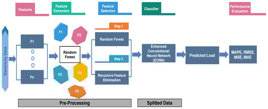
Figure 1. Proposed Model for Load Prediction.

• Feature Extraction
• Feature Selection
• Load prediction using ECNN
• Performance evaluation

3.1.1. Data Source

Independent System Operator New England (ISO-NE) [45] is an electric power industry. It generates, transmits and distributes electricity to the industrial, residential and commercial area. ISO-NE generates a large amount of data about load, price, generation and distribution, etc. Load data of 2018 is taken from ISO-NE, which is used in the implementation of proposed models.

3.1.2. Feature Extraction

Feature extraction is a process used to extract some features from the dataset. In this process, a subset (new data is generated according to original data) of the data is selected to give more accurate results than original data [4]. In literature, different techniques are used to extract features from data. RFE is used for feature extraction in the proposed model.

3.1.3. Feature Selection

Feature selection is a process used to select more relevant features [46]. It reduces the number of features from the dataset. RF is used to calculate the importance of every feature. Basically, it is done to eliminate the less important features. A hybrid approach which is the combination of RFE and RF is proposed for final selection. The proposed approach outperformed the existing approaches.

3.1.4. ECNN

CNN is a type of deep neural network. It lies in the class of supervised DL models [13]. First, sequential model is used to implement ECNN. It creates a layer-by-layer model. In this model, four different layers are used to build a network for prediction. Convolution layer is added as a second layer to check the output neurons that are connected to the input. The input of convolutional layer is $m\times r$. Where m is the height and r is the width of the matrix. Kernel size is used as a filter in which dimension of matrix is smaller than the dataset. It gives the feature mapping function. Here, 2 is used as a kernel size or filter for feature mapping. Where size of filter provides the connected structure of the network. In addition, Relu is used as an activation function and is calculated using Equation (1). Where x is the input data, Relu returns 0 if the input is negative and return the same value if x is non-negative.

$$Relu\left(x\right)=max(0,x)$$

(1)

Afterwards, max-pooling is used as a third layer in the network which provides matrix with small values. For instance, max pooling selects the highest values from the different matrices. Then create a small matrix from these values. Table 2 shows the formula to calculate the output size of convolutional layer.

Table 2. Output Calculation for Convolutional Layer.

Input	Filter	Output
$n\times n$	$f\times f$	${(n+2pf+1)}^2$

Where p is padding, f is the number of filters and n is input size for example: $32\times 32\times 1$. Dropout layer is used as fourth layer to avoid the over-fitting problem. Flatten layer is used to convert all the neurons into a single connected layer. Then comes the application of the dense layer to perform classification. Each node is connected to all other nodes. Early stopping finds the loss rate value of neurons. If the early stopping does not find the value of loss rate of a network in a stable state then it will check it again. Then, one moves to the dropout layer to avoid over fitting problem and again apply the dense layer. At last, the output layer shows the result of the prediction. In this model, ‘Adam’ is used as an optimizer. In this paper, ECNN predicts the load and price of electricity with different scenarios. The stepwise flow of the proposed model is shown in Algorithm 1.

Algorithm 1 Electricity Load Forecasting Model

Input: Electricity load data

/* Separate target from features */

1: X: features of data

2: Y: target data

/* Split data into training and testing */

3: x_train, x_test, y_train, y_test = split(x, y);

4: Combine_imp = DT − imp + XG − imp;

/* Calculate importance using Random Forest */

5: RF_imp = importance calculate by RF;

/* Feature extraction using RFE */

6: Selected_ feature = RFE(5, x_train, y_train);

/* Hybrid feature selection */

7: if (Combine_imp ≥ threshold And RFE == true) then

8:  Reserve feature;

9: else

10:  Drop feature;

11: end if

12: Prediction using ESVM and ECNN with tuned parameters

13: Compare predictions with y_test;

3.2. Electricity Price Forecasting Model

The model for price prediction is shown in Figure 2. The model is divided into four modules:

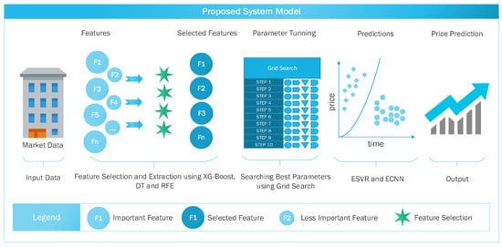
Figure 2. Proposed Model for Price Prediction.

• Feature Selection
• Feature Extraction
• GS and cross-validation
• Price Prediction using ESVR and ECNN

The individual modules are further explained in the following subsections.

3.2.1. Model Overview

The accuracy of prediction is a key issue in electricity price forecasting. As discussed earlier, the electricity price depends on various factors, which make training of classifiers difficult. To improve the accuracy of price prediction, hybrid feature selector (i.e., DTC and XG-boost) is used to select the most relevant features. First, RFE is used to remove dimensionality and redundancy of data. In order to tune parameters of the classifier, GS is used along with cross-validation to select the best subset of parameters. Finally, selected features and the best parameters are used in classifiers to predict electricity price.

3.2.2. Feature Extraction Using RFE

RFE is used to select a specified number of features from the dataset. It removes the weakest feature recursively till the specified number of features reached. RFE requires several features to select; however, it is difficult to decide in advance that how many features are most relevant. To address this issue, cross-validation is used with RFE. Cross-validation calculates the accuracy of different subsets and selects the subset with the highest accuracy.

3.2.3. Feature Selection Using XG-Boost and DT

XG-boost and DT are used to calculate the importance of all features with respect to the target, i.e., electricity price. These techniques calculate the importance of features in vector form. The components of this vector represent the importance of every feature in the sequence. However, less important features can be dropped. The fusion of XG-boost and DT gives more accurate results. In simulation and results the importance of features shows in the form of bar graph. To control feature selection, threshold $ϵ$ is used. Features having importance greater than or equal to the threshold $ϵ$ are considered and rest of the features are dropped. Feature selection is performed using Equations (2) and (3) as:

$$Fs=\mathrm{Reserve}\mathrm{if}{I}_{XG}\left[i\right]+I_{DT}\left[i\right]\ge ϵ$$

(2)

$$\mathrm{Drop}\mathrm{if}{I}_{XG}\left[i\right]+I_{DT}\left[i\right]<ϵ$$

(3)

where, $I_{XG}\left[i\right]$ represents the feature importance calculated by XG-boost, $I_{DT}\left[i\right]$ is the feature importance calculated by DT. $ϵ$ is a threshold value for the feature selection and i represents features.

3.2.4. Tuning Hyper-Parameters and Cross-Validation

Tuning of a classifier is very important to do accurate and efficient forecasting. There is a strong relationship between hyper-parameter and results of the classifier. GS is used to tune the parameters of a classifier for high accuracy. For this purpose, we define a subset of parameter of SVR and CNN as shown in Table 3 and Table 4, respectively. After that, GS is performed to find the parameter values having less loss function. The results of the GS are verified by k-fold cross-validation.

Table 3. Subset of ESVR Parameters for GS.

Parameter Name	Parameter Values	Description
kernel	[‘linear’, ‘rbf’]	Kernel for Support Vector Machine
C	[3, 5, 10, 15, 20, 30]	C is a regularization parameter that controls the trade off between the achieving a low training error and a low testing error
gamma	[‘scale’, ‘gamma’, 10, 20, 30]	It is the inverse of the standard deviation, which is used as similarity measure between two points
epsilon	[0.2, 0.02, 0.002, 0.0002]	It is used to denote error margin, in terms of regressive functional loss

Table 4. Subset of ECNN Parameters for GS.

Parameter Name	Parameter Values	Desription
batch_size	[10, 20, 40, 50, 60]	The batch size defines the number of samples
epochs	[10, 30, 50, 70, 100, 150	Number of iterations
learning_rate	[0.001, 0.01, 0.1, 0.2, 0.3]	Defined in the context of optimization, and minimizing the loss function of a neural network
activation	[‘softmax’, ‘relu’, ‘sigmoid’, ‘linear’]	Defines the output of a specific node
optimizer	[‘SGD’, ‘Adam’, ‘Adamax’, ‘Nadam’]	Update network weights iteratively to minimize the loss function
dropout_rate	[0.0, 0.1, 0.2, 0.3, 0.4, 0.5]	Dropout rate is a guidance for hidden layers to avoid over-fitting

3.2.5. Electricity Price Forecasting

After feature selection and parameter tuning, the processed data and the best subset of parameters are used in ESVR and ECNN to forecast electricity price. Hourly price data of two months (November and December 2016) are used to train the classifier and predicts the price for the first week of January 2017. We compared the results of 1 January 2017 and first week of January 2017 with the actual price of electricity of NYISO. ESVR provides better results which can be envisioned in Section 5.3.4 Price prediction. The results of ESVR are close to the blue line which shows better price accuracy. Whereas, results of ECNN are also shown in figures. In these figures, the yellow line is very close to the blue line, which shows that prediction is close to the real price.

The complete flow of the proposed model for electricity price prediction is shown in Algorithm 2.

Algorithm 2 Electricity Price Forecasting Model

Input: Electricity price data;

/* Separate target from features */

1: X: features of data;

2: Y: target data;

/* Split data into training and testing */

3: x_train, x_test, y_train, y_test = train_test_split(x, y);

/* Feature extraction using RFE */

4: Selected_ feature = RFE(9, x_train, y_train);

/* Hybrid Feature Selection */

5: DT_imp = importance calculate by DT; C

6: XG_imp = importance calculate by XG − boost;

7: Combined_imp = DT_imp + XG_imp;

8: if (combined_imp ≥ ϵ) then

9:  Reserve feature;

10: else

11:  Drop feature;

12: end if

13: Grid Search for parameter tuning;

14: Prediction using ESVR and ECNN with tuned parameters;

15: Compare predicted price with actual price;

4. Classifiers and Techniques

In this section, classifiers and the proposed techniques are described briefly:

4.1. XG-Boost

Extreme Gradient Boosting (XG-boost) is an optimized gradient boosting library. It is designed to be highly portable, flexible and efficient. It works under the gradient boosting framework and provides parallel tree boosting to solve the problems of classification efficiently and accurately. It is used to solve regression, classification and ranking problems. It is an open source library. It is available in different languages i.e., R, Python, C++ and for different operating systems, i.e., Windows, Linux and OSX.

4.2. DT

DT is a supervised machine learning algorithm used for decision making, classification and regression. According to certain parameters, the data is continuously split into different nodes of the tree. The two main entities in DT are decision nodes and leaf nodes (leaves). The decision nodes are those points where data splits and leaf nodes are final outcomes or decisions.

4.3. RFE

RFE is a feature selection method used to remove the less important features. It removes the weakest feature recursively till the specified number of features reached. RFE calculates the importance of features. Using this importance, features are eliminated recursively. It also eliminates the co-linearity and dependencies that may exist in this model. RFE select features according to the specified number of features. However, we cannot decide in advance how many features are optimal for prediction. In order to resolve the aforementioned problem, cross-validation is used to select an optimal number of features. Cross-validation is used to score the subsets of different features. It also selects the subset of features with the highest score.

4.4. RF

RF is an ensemble learning method used to solve classification, regression and other decision making problems. It easily deals with the missing values of data. It consists of more than one decision trees. It works on rule-based system. In addition, it combines the prediction of many decision trees as well as bootstrapping and bagging principles. Bagging means to select values randomly from the training values. For clarification, bootstrapping means that the sample(s) chosen from the training set.

4.5. Cross-Validation

Cross-validation is a technique used to estimate and test the performance of model on the subsets of available input. In addition, cross-validation is used to avoid over-fitting. K-fold is a well-known technique for cross-validation. In this process, input data is divided into K subsets (also known as folds). Model is trained on K − 1 subsets and validates the results on the subset that is not used in training. The process is repeated K times, by selecting different subset for validation each time.

4.6. GS

GS is the traditional way to tune the parameters for optimization. GS performs an exhaustive search through defined set of learning algorithm parameters. Furthermore, it requires some performance metrics to calculate accuracy of a classifier for every subset of parameters. The classifiers use subset of parameters having the highest accuracy.

4.7. ESVR

SVM is a supervised learning model used for both regression and classification. The main objective of SVM is to find hyperplane between n-dimensions, where n is the number of features. Hyperplane distinctly classify the data. SVM has two functions: Support Vector Regression (SVR) to do regression and Support Vector Classifier (SVC) for classification.

In this paper, an enhanced SVR is proposed by tuning parameters dynamically using GS. The flowchart of the ESVR is graphically represented in Figure 3. After feature selection and extraction, a subset of parameters is defined in the range of SVM parameters. Using this subset, all possible combination of parameters are defined. Each combination is applied to the classifier and the fitness of this combination is calculated by applying k-fold cross-validation. After applying all combinations of parameters, an algorithm will obtain the combination of parameters having the highest fitness and pass it to ESVR. ESVR is then trained using training data to get prediction results. Simulation results show that ESVR outperformed in our scenario.

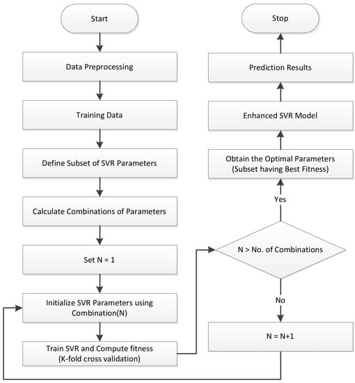
Figure 3. Enhanced Support Vector Regression.

4.8. ECNN

CNN is a commonly used DL method. It lies in the class of supervised learning. In this paper, an enhanced CNN model is proposed by adding layers in specific structure to increase the accuracy in prediction. The flowchart of ECNN is shown in Figure 4. The layers of ECNN are discussed in the following subsections.

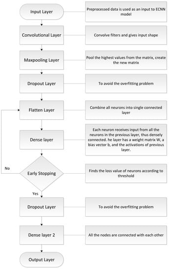
Figure 4. Enhanced Convolutional Neural Network.

4.8.1. Input Layer

The input layer is the beginning of the work-flow for the CNN. It is the first layer of network. This layer does not take any input from previous layer. The input layer does not have weighted inputs. The number of neurons at input layer is equal to the number of features in dataset.

4.8.2. Hidden Layer

The hidden layer is the second layer of the model. The values are passed from input to hidden layer. In CNN, one or more hidden layers are used according to the requirement. Each hidden layer has a different number of neurons. These neurons are generally greater than the number of features. The output of this layer is calculated through matrix multiplication of weights and output of the previous layer. The bias weights are also added to the output.

4.8.3. Output Layer

The values obtained from hidden layer is considered as an input of output layer. The logistic function i.e., sigmoid or softmax is used to convert the output into probability score of each class.

4.8.4. Convolution Layer

The building block of CNN is convolutional layer that performs most of the computations of a model. The convolution layer consists of several filters. It performs a convolution operation on the input and passes the results to the next layer.

4.8.5. Pooling Layer

Pooling layer is used to combine the output of neurons. It is further divided into three types:

• Max Pooling
• Average Pooling
• Sum Pooling

In this paper, the max pooling layer is used to reduce the number of parameters and amount of computation in the network. In addition, it also controls over-fitting. It is commonly inserted between the convolutional layer and dropout layer.

4.8.6. Activation Function

In convolutional layer, Rectified Linear Unit (Relu) used as an activation function. The equation used for Relu is give in Equation (1).

4.8.7. Work Flow of ECNN

The working of ECNN is shown in Figure 4. First, the data is in normalized form which is taken as input after preprocessing steps. Then, the convolutional layer is used to apply filters and convolve the large input into small matrix. Afterwards, one used max pooling layer to collect the highest values of each matrix from the pool and create a new small matrix. Then, one applies the dropout layer to avoid over-fitting problem. It also reduced the computational time. The flattened layer is used to connect all the neurons from the previous layer. The dense layer is used to connect all the nodes with eachother. One applies the early stopping function which tells the loss rate values of neurons during connection from one layer to another layer. If the loss rate value is more than the threshold value, it will go back to dense layer and try to connect maximum nodes with eachother. If the loss value of neurons are less than threshold value, it will move further to dropout layer to prevent over-fitting problem in a network. The dense layer acts as a fully connected layer. Then, the output layer shows the results of the fully connected layer.

4.9. Performance Evaluators

The proposed models are evaluated on the basis of performance metrics: Mean Average Percentage Error (MAPE), Root Mean Square Error (RMSE), Mean Square Error (MSE) and Mean Absolute Error (MAE). The formulas of MSE, MAE, RMSE and MAPE are given in Equations (4)–(7) [22]. Table 5 shows the evaluation of performance metrics of different techniques on the data set of ISO-NE.

$$\mathrm{MAPE}=\frac{1}{T}\sum _{tm=1}^{TM}100\left|\frac{A_v-F_v}{A_v}\right|$$

(4)

$$\mathrm{RMSE}=\sqrt{\frac{1}{T}\sum _{tm=1}^{TM}{(A_v-F_v)}^2}$$

(5)

$$\mathrm{MSE}=\frac{1}{T}\sum _{tm=1}^{TM}{(A_v-F_v)}^2$$

(6)

$$\mathrm{MAE}=\frac{{\sum }_{tm=1}^{TM}\left|(F_v-A_v)\right|}{T}$$

(7)

where $A_v$ is the actual value at time TM and $F_v$ is the forecasted value at time TM.

Table 5. Performance Evaluation Metrics for Load Prediction Model.

Dataset	Technique	MAE	MAPE	MSE	RMSE
ISO-NE	SVR	2.84	6.21	7.87	2.80
	ESVR	2.11	5.3	6.72	2.59
	CNN	3.12	37.32	7.23	2.68
	ECNN	2.43	34.78	4.01	2.00

5. Simulation and Results

In this section, the simulation results are discussed in detail.

5.1. Simulation Environment

For simulation purposes, the proposed models are implemented by using the following Python libraries i.e., Keras, Tensorflow, Sklearn, numpy and pandas. Models are implemented on a system with Intel core i3, 8 GB RAM and 500 GB storage capacity. Two different datasets are selected for simulation. Dataset 1 is used for a load prediction model, which is taken from ISO-NE and it contains hourly data of a load of electricity. Where dataset 2 is used as input in the price prediction model, which is taken from NYISO. However, dataset 2 contains hourly data of price and electricity generation from 2016–2017.

5.2. Results of Load Prediction Model

The results are generated in the form of graphs after performing simulations on the dataset of ISO-NE. These graphs show the comparison of actual load with predicted load.

Figure 5 shows the importance of all features. Importance of features show the correlation among different features with target class. It shows the best features which are selected from large dataset. In addition, it shows that some features have high importance while others have comparatively less importance. For simulations, the value of threshold is 0.08 which is used to select the most relevant features.

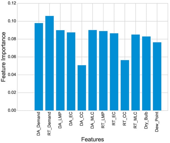
Figure 5. Feature Importance.

Figure 6 shows the load prediction of ECNN. In this figure, blue line shows the actual load of 2018 and yellow line represents the predicted load. Prediction of ECNN depicts that the predicted load is nearly close to the actual load.

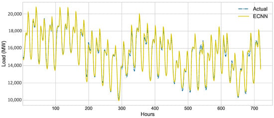
Figure 6. Load Prediction using ECNN.

Figure 7 shows the day ahead predicted load. The blue line shows the actual load of one day and yellow line represents the predicted load of one day. The comparison of actual and predicted load shows that the prediction of ECNN is accurate and acceptable.

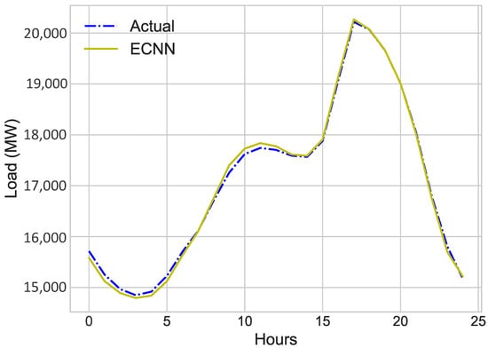
Figure 7. Day-Ahead Load (MW) Jan 2018.

Figure 8 shows the prediction of one week of January 2018 and actual weekly load consumption of January 2018. From simulation results, the spikes show the variations in load and the consumption pattern of electricity.

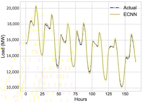
Figure 8. One Week Load Prediction.

The consumption behavior of electricity of all months are different. It means that the consumption of electricity depends on other various factors. Figure 9 shows the comparison of actual load consumption of January and September 2018. It is concluded that the consumption of electricity is not same for all months. The electricity load consumption varies according to the weather and status of the day (whether it is working day or holiday). It also varies from time to time. Figure 10 shows the actual normalized load of electricity.

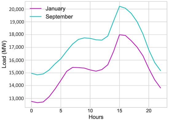
Figure 9. Hourly Load (MW) of January and September 2018.

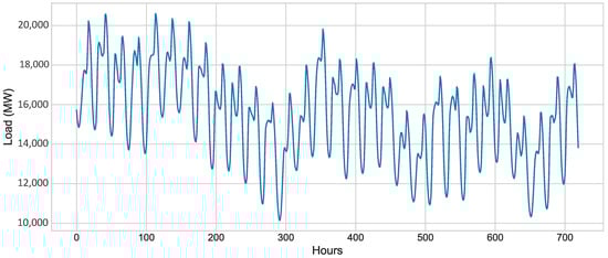
Figure 10. Actual load.

Comparison of proposed models: ESVR, ECNN and actual load is shown in Figure 11. It shows the comparison of benchmark schemes with the proposed model. This figure represents the actual and predicted load of ECNN and SVM, respectively. The percentage of error value of the prediction for ECNN is less than other benchmark schemes as given in Table 6. It indicates that ECNN outperformed other benchmark schemes.

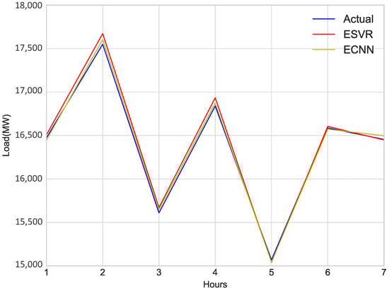
Figure 11. Day ahead Comparison of Load.

Table 6. Performance Evaluation Metrics for Price Prediction Model.

Dataset	Technique	MAE	MAPE	MSE	RMSE
NYISO	SVR	1.88	4.59	6.22	2.49
	ESVR	1.78	4.2	5.23	2.28
	CNN	2.51	34.12	5.11	2.26
	ECNN	1.38	32.08	3.22	1.79

5.3. Results of Price Prediction Model

The results of price prediction model are discussed in this section. NYISO dataset (Dataset 2) is taken as input, which contains 9314 real-world records. However, for the sake of demonstration, 75 days dataset is used to train model. This dataset invariably contains approximately 2000 h record, i.e., from 1 November 2016 to 15 January 2017. The whole simulation process is organized as:

• Feature extraction using RFE
• Feature selection by combining the importance of attributes calculated by XG-boost and DT
• Parameter tuning using cross-validation and GS
• Prediction using ESVR and ECNN
• Results and Comparison with real data of January 2017

5.3.1. Feature Extraction

RFE is used to remove redundancy and dimensionality of data. However, it is difficult to determine in advance that how many feature sets are required. To resolve this issue, cross-validation is used with RFE to select optimal number of features. Cross-validation tests every combination of features and calculates the accuracy of each subset. The subset of features with the highest accuracy is used for prediction. Figure 12 shows the maximum accuracy score on eight number of features.

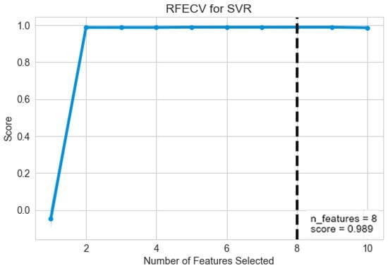
Figure 12. Result of Cross-validation (RFE).

5.3.2. Feature Selection

Importance of selected features are calculated by both DT and XG-boost. By adding both importance and combined importance is calculated. For selection of features, a threshold value $ϵ$ is defined. Features are selected having importance greater than or equal to threshold value. Figure 13 shows the importance of every feature. Some features have very high importance, i.e., TWI Zonal LBMP, RTC Zonal LBMP and Load. TWI zonal price version shows very less importance as compared to the other features. Most of the features have importance greater than 0.15. The value of threshold is 0.15 because of the aforesaid reason. The features having values less than threshold are dropped.

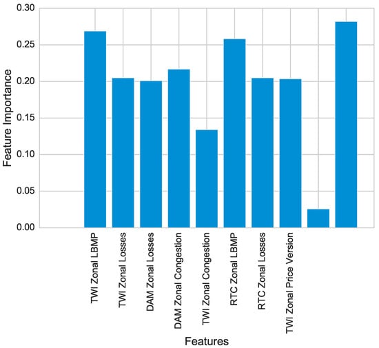
Figure 13. Feature Importances for Price.

5.3.3. Parameter Tuning and Cross-Validation

There is a strong relationship between hyper-parameters and results of the classifiers. To tune parameters of the classifier, a subset of hyper-parameters is defined for classifiers as given in Table 3 and Table 4. The parameters with a large effect on the results are taken into consideration and the range of their values is defined on test and trail basis. After that, GS is applied to find the set of values of parameters in order to minimize the loss function. However, the GS is an exhaustive search. It increases the execution time and computation overhead. To resolve the aforesaid issue, a small sample data is selected to perform a GS which boosts the speed of GS. The results of GS are verified by k-fold cross-validation. After tuning classifiers, prediction is performed and explained in the next subsection.

5.3.4. Price Prediction

Hourly data of November and December 2016 is used to train the classifiers. ESVR and ECNN are used to predict price of electricity for first week of January. To verify the accuracy of model, predicted price is compared with the actual price of first week of January. The results of price prediction are shown in Figure 14 and Figure 15. These figures show both actual and predicted price for 1 January 2017 and first week of January, 2017. Figure 14 and Figure 16 depicts the prediction of ESVR. While results of ECNN can be envisioned from Figure 15 and Figure 17.

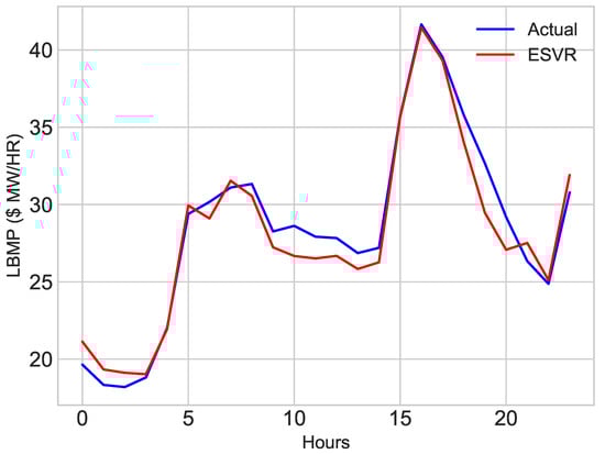
Figure 14. First Week of January, 2017.

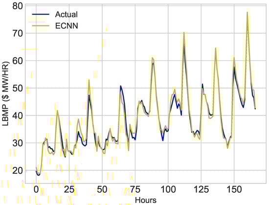
Figure 15. First Week of January, 2017.

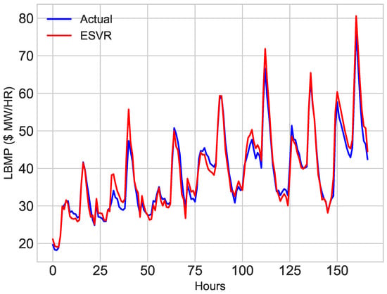
Figure 16. First Week of January, 2017.

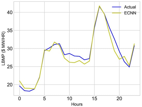
Figure 17. First Week of January, 2017.

5.4. Discussion of Results

The sole purpose of the proposed model is to improve the accuracy of classifiers to predict price and load optimally. The results before parameter tuning of the classifier are less accurate as shown in Figure 18 and Figure 19. The error rate of prediction for MAE before parameter tuning is approximately equal to 2.83. The results are improved after feature selection, extraction and parameter tuning through GS. The results after parameter tuning of ESVR are shown in Figure 14 and Figure 16. The results of ECNN are shown in Figure 15 and Figure 17. After parameter tuning, the accuracy of classifiers is improved and the error rate for MAE is reduced to 1.81. The comparison of actual values, before and after tuning classifiers is shown in Figure 20 and Figure 21. From the simulation results, it is concluded that MAE is decreased after performing parameter tuning and the results are improved. Simulation results confirmed that after reducing the error by 1% also reduced the energy consumption. It also minimized the electricity cost.

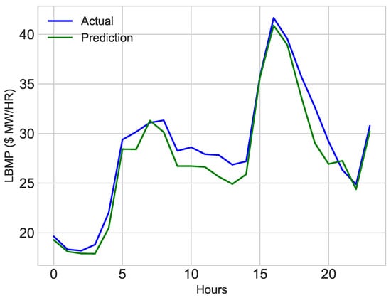
Figure 18. First Day of January, 2017.

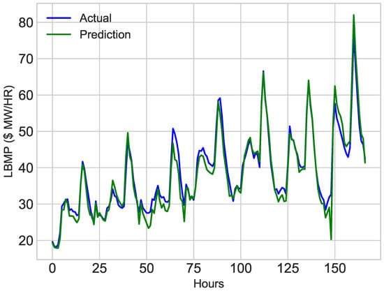
Figure 19. First Week of January, 2017.

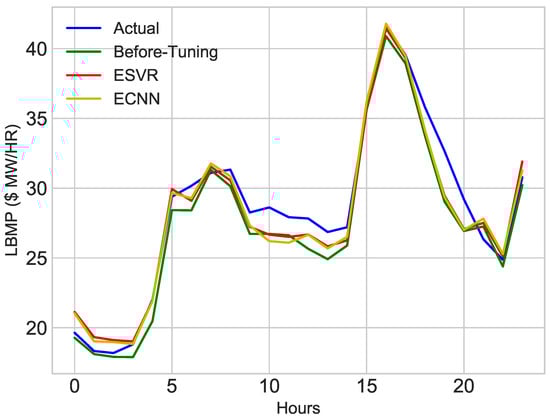
Figure 20. 1 January 2017.

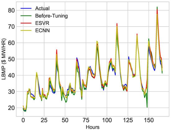
Figure 21. First Week of January, 2017.

5.4.1. Effect of Hybrid Feature Selection Technique on Prediction

In this paper, a hybrid feature selection technique is proposed. We can control feature selection by changing the threshold value. Feature selection has a great impact on the accuracy of prediction. In order to adjust the threshold value, some tests are performed by changing the threshold value of the hybrid feature selection technique. The threshold values and their corresponding results are shown in Figure 22. The threshold value is 0.15 because there is a less error rate on it. The error rate on threshold 0.25 is also less; however, the number of features selected on 0.15 is less than 0.25. It also decreased the execution time. If the threshold is 0.15, it reduced the error rate and features. The proposed approach efficiently increased the accuracy and reduced the execution time. It also minimized the computation overhead optimally.

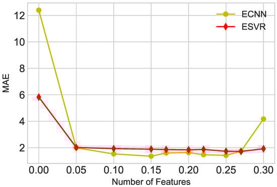
Figure 22. Effect of Hybrid Feature selector.

5.4.2. Comparison of Techniques

The proposed models are compared with existing benchmark schemes to verify the adaptivity of the proposed models. The benchmark schemes are AdaBoost (AB), Multilayer Perceptron and RF. The comparison results are given in Table 7. After performing two-step feature selection, the aforementioned techniques are applied to the dataset. Figure 23 depicts the results of the aforementioned classifiers. The results of all classifiers are satisfactory; however, ECNN and ESVR outperformed other classifiers. The results of other classifiers are also close to the actual values; however, the overall results of ECNN and ESVR are better than AB, MLP and RF. Figure 24 shows the comparison of different techniques on performance metrics.

Table 7. Comparison of Proposed Model with other Benchmark Schemes.

Techniques	MAE	MAPE	MSE	RMSE
ESVR	1.00	3.70	1.54	1.24
ECNN	0.99	18.18	1.64	0.99
AdaBoost (AB)	1.74	7.02	4.58	1.31
Multi Layer Perceptron (MLP)	1.43	4.90	3.06	1.19
Random Forest (RF)	1.91	7.31	5.40	1.38

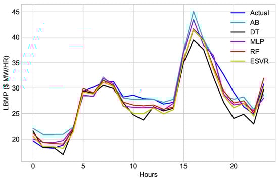
Figure 23. Comparison of proposed models with benchmark schemes.

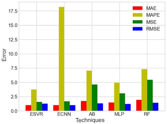
Figure 24. Performance metrics of different techniques.

5.4.3. Effect of Dataset Size on Accuracy

DL models required a large amount of data for training. We investigated the performance and accuracy of the proposed models on different size of the datasets. To identify the behavior of proposed model on different sizes of dataset, a dataset is divided into three categories i.e., small (2000 rows), medium (4000 rows) and large (6000 rows). Furthermore, the simulations are performed on each dataset, the results of the simulations are mentioned in Table 8. The values of error decrease with an increase in data size; especially in the case of ECNN, the error rate decrease with an increase in data size. These results show that the proposed models performed well on both small and large datasets. Furthermore, the execution time of the proposed models is also decreased using two-step feature extraction and selection.

Table 8. Effect of Size of Dataset on Performance.

Dataset Size	No. of Records	Technique (s)	MAE	MAPE	MSE	RMSE
Small	2000	ECNN	1.67	32.12	3.80	1.94
		ESVR	1.78	4.60	4.78	2.18
Medium	4000	ECNN	1.65	32.39	4.92	2.21
		ESVR	1.75	4.50	4.94	2.22
Large	6000	ECNN	1.46	18.17	3.54	1.88
		ESVR	1.74	4.50	4.94	2.22

6. Conclusions and Future Studies

In this paper, two models are proposed: one for electricity load prediction and the other for electricity price prediction. The primary goal is to increase the accuracy of forecasting using these models. For better accuracy, data pre-processing (feature selection and extraction) and parameter tuning of classifiers are done using GS and cross-validation. The simulation results and values of performance metrics show that the proposed models are more accurate than the benchmark schemes.

In these models, a hybrid feature selection technique is used to select the best features from the dataset. RFE is used to eliminate the redundancy of data and reduced the dimensionality. Enhanced classifiers (ECNN and ESVR) are used to predict price and load of electricity. It also reduced the over-fitting problem and minimized the execution and computation time. Stability analysis is also performed to check the stability of the proposed models using different data sizes.

Table 9 shows all the abbreviations used in this paper. In future, we will enhance the classifiers to provide optimal results. Furthermore, different classifier with meta-heuristic techniques will be used to provide accuracy.

Table 9. Table of Abbreviations.

Abbreviation(s)	Description(s)
ANN	Artificial Neural Network
BPNN	Back Propagation Neural Network
CNN	Convolutional Neural Network
DA	Data Analytic
DNN	Deep Neural Network
DR	Demand Response
DT	Decision Tree
FE	Feature Extraction
FS	Feature Selection
GCA	Grey Correlation Analysis
GELM	Generalize Extreme Learning Machine
KNN	K-Nearest Neighbor
KPCA	Kernel Principal Component Analysis
LR	Logistic Regression
LSTM	Long Short Term Memory
LTLF	Long-Term Load Forecasting
MAE	Mean Absolute Error
MAPE	Mean Absolute Percentage Error
MSE	Mean Square Error
STELF	Short-Term Electricity Load Forecasting
STLF	Short-Term Load Forecasting
MTLF	Medium-Term Load Forecasting
MLP	Multi Layer Perceptron
NYISO	New York Independent System Operator
RELU	Rectified Linear Unit
RF	Random Forest
RFE	Recursive Feature Elimination
RMSE	Root Mean Square Error
SDA	Stacked De-noising Auto-encoder
SG	Smart Grid
SM	Smart Meter
SVM	Support Vector Machine
SVR	Support Vector Regression
ESVR	Enhanced Support Vector Regression
TG	Traditional Grid

References

- Masip-Bruin, X.; Marin-Tordera, E.; Jukan, A.; Ren, G.J. Managing resources continuity from the edge to the cloud: Architecture and performance. Future Gener. Comput. Syst. 2018, 79, 777–785. [Google Scholar] [CrossRef]
- Osman, A.M. A novel big data analytics framework for smart cities. Future Gener. Comput. Syst. 2019, 91, 620–633. [Google Scholar] [CrossRef]
- Chen, X.-T.; Zhou, Y.-H.; Duan, W.; Tang, J.-B.; Guo, Y.-X. Design of intelligent Demand Side Management system respond to varieties of factors. In Proceedings of the 2010 China International Conference on Electricity Distribution (CICED), Nanjing, China, 13–16 September 2010; pp. 1–5. [Google Scholar]
- Bilalli, B.; Abelló, A.; Aluja-Banet, T.; Wrembel, R. Intelligent assistance for data pre-processing. Comput. Stand. Interfaces 2018, 57, 101–109. [Google Scholar] [CrossRef]
- Mohsenian-Rad, A.-H.; Leon-Garcia, A. Optimal residential load control with price prediction in real-time electricity pricing environments. IEEE Trans. Smart Grid 2010, 1, 120–133. [Google Scholar] [CrossRef]
- Chandrashekar, G.; Sahin, F. A survey on feature selection methods. Comput. Electr. Eng. 2017, 40, 16–28. [Google Scholar] [CrossRef]
- Erol-Kantarci, M.; Mouftah, H.T. Energy-efficient information and communication infrastructures in the smart grid: A survey on interactions and open issues. IEEE Commun. Surv. Tutor. 2015, 17, 179–197. [Google Scholar] [CrossRef]
- Wang, K.; Li, H.; Feng, Y.; Tian, G. Big data analytics for system stability evaluation strategy in the energy Internet. IEEE Trans. Ind. Inform. 2017, 13, 1969–1978. [Google Scholar] [CrossRef]
- Wang, K.; Ouyang, Z.; Krishnan, R.; Shu, L.; He, L. A game theory-based energy management system using price elasticity for smart grids. IEEE Trans. Ind. Inform. 2015, 11, 1607–1616. [Google Scholar] [CrossRef]
- Wang, H.Z.; Li, G.Q.; Wang, G.B.; Peng, J.C.; Jiang, H.; Liu, Y.T. Deep learning based ensemble approach for probabilistic wind power forecasting. Appl. Energy 2017, 188, 56–70. [Google Scholar] [CrossRef]
- Mosbah, H.; El-Hawary, M. Hourly electricity price forecasting for the next month using multilayer neural network. Can. J. Electr. Comput. Eng. 2016, 39, 283–291. [Google Scholar] [CrossRef]
- Hu, Q.; Zhang, R.; Zhou, Y. Transfer learning for short-term wind speed prediction with deep neural networks. Renew. Energy 2016, 85, 83–95. [Google Scholar] [CrossRef]
- Kuo, P.H.; Huang, C.J. An Electricity Price Forecasting Model by Hybrid Structured Deep Neural Networks. Sustainability 2018, 10, 1280. [Google Scholar] [CrossRef]
- Ugurlu, U.; Oksuz, I.; Tas, O. Electricity Price Forecasting Using Recurrent Neural Networks. Energies 2018, 11, 1255. [Google Scholar] [CrossRef]
- Eapen, R.R.; Simon, S.P. Performance Analysis of Combined Similar Day and Day Ahead Short Term Electrical Load Forecasting using Sequential Hybrid Neural Networks. IETE J. Res. 2018. [Google Scholar] [CrossRef]
- Zhang, X.; Wang, J.; Zhang, K. Short-term electric load forecasting based on singular spectrum analysis and support vector machine optimized by Cuckoo search algorithm. Electr. Power Syst. Res. 2017, 146, 270–285. [Google Scholar] [CrossRef]
- Patil, M.; Deshmukh, S.R.; Agrawal, R. Electric power price forecasting using data mining techniques. In Proceedings of the 2017 International Conference on Data Management, Analytics and Innovation (ICDMAI), Pune, India, 24–26 February 2017; pp. 217–223. [Google Scholar]
- Bouktif, S.; Fiaz, A.; Ouni, A.; Serhani, M. Optimal deep learning lstm model for electric load forecasting using feature selection and genetic algorithm: Comparison with machine learning approaches. Energies 2018, 11, 1636. [Google Scholar] [CrossRef]
- Ziming, M.A.; Zhong, H.; Le, X.I.; Qing, X.I.; Chongqing, K.A. Month ahead average daily electricity price profile forecasting based on a hybrid nonlinear regression and SVM model: An ERCOT case study. J. Mod. Power Syst. Clean Energy 2018, 6, 281–291. [Google Scholar]
- Lago, J.; de Ridder, F.; de Schutter, B. Forecasting spot electricity prices: Deep learning approaches and empirical comparison of traditional algorithms. Appl. Energy 2018, 221, 386–405. [Google Scholar] [CrossRef]
- Ghadimi, N.; Akbarimajd, A.; Shayeghi, H.; Abedinia, O. Two stage forecast engine with feature selection technique and improved meta-heuristic algorithm for electricity load forecasting. Energy 2018, 161, 130–142. [Google Scholar] [CrossRef]
- Jindal, A.; Singh, M.; Kumar, N. Consumption-Aware Data Analytical Demand Response Scheme for Peak Load Reduction in Smart Grid. IEEE Trans. Ind. Electron. 2018. [Google Scholar] [CrossRef]
- Chitsaz, H.; Zamani-Dehkordi, P.; Zareipour, H.; Parikh, P. Electricity price forecasting for operational scheduling of behind-the-meter storage systems. IEEE Trans. Smart Grid 2018, 9, 6612–6622. [Google Scholar] [CrossRef]
- Pérez-Chacón, R.; Luna-Romera, J.M.; Troncoso, A.; Martínez-Álvarez, F.; Riquelme, J.C. Big Data Analytics for Discovering Electricity Consumption Patterns in Smart Cities. Energies 2018, 11, 683. [Google Scholar] [CrossRef]
- Wang, Z.; Wang, Y.; Zeng, R.; Srinivasan, R.S.; Ahrentzen, S. Random Forest based hourly building energy prediction. Energy Build. 2018, 171, 11–25. [Google Scholar] [CrossRef]
- Lahouar, A.; Slama, J.B.H. Day-ahead load forecast using random forest and expert input selection. Energy Convers. Manag. 2015, 103, 1040–1051. [Google Scholar] [CrossRef]
- Wang, K.; Xu, C.; Zhang, Y.; Guo, S.; Zomaya, A. Robust big data analytics for electricity price forecasting in the smart grid. IEEE Trans. Big Data 2017. [Google Scholar] [CrossRef]
- Wang, L.; Zhang, Z.; Chen, J. Short-term electricity price forecasting with stacked denoising autoencoders. IEEE Trans. Power Syst. 2017, 32, 2673–2681. [Google Scholar] [CrossRef]
- Lago, J.; de Ridder, F.; Vrancx, P.; de Schutter, B. Forecasting day-ahead electricity prices in Europe: The importance of considering market integration. Appl. Energy 2018, 211, 890–903. [Google Scholar] [CrossRef]
- Raviv, E.; Bouwman, K.E.; van Dijk, D. Forecasting day-ahead electricity prices: Utilizing hourly prices. Energy Econ. 2015, 50, 227–239. [Google Scholar] [CrossRef]
- Mujeeb, S.; Javaid, N.; Akbar, M.; Khalid, R.; Nazeer, O.; Khan, M. Big Data Analytics for Price and Load Forecasting in Smart Grids. In International Conference on Broadband and Wireless Computing, Communication and Applications; Springer: Cham, Switzerland, 2018; pp. 77–87. [Google Scholar]
- Rafiei, M.; Niknam, T.; Khooban, M.-H. Probabilistic forecasting of hourly electricity price by generalization of ELM for usage in improved wavelet neural network. IEEE Trans. Ind. Inform. 2017, 13, 71–79. [Google Scholar] [CrossRef]
- Abedinia, O.; Amjady, N.; Zareipour, H. A new feature selection technique for load and price forecast of electrical power systems. IEEE Trans. Power Syst. 2017, 32, 62–74. [Google Scholar] [CrossRef]
- Ghasemi, A.; Shayeghi, H.; Moradzadeh, M.; Nooshyar, M. A novel hybrid algorithm for electricity price and load forecasting in smart grids with demand-side management. Appl. Energy 2016, 177, 40–59. [Google Scholar] [CrossRef]
- Shayeghi, H.; Ghasemi, A.; Moradzadeh, M.; Nooshyar, M. Simultaneous day-ahead forecasting of electricity price and load in smart grids. Energy Convers. Manag. 2015, 95, 371–384. [Google Scholar] [CrossRef]
- Keles, D.; Scelle, J.; Paraschiv, F.; Fichtner, W. Extended forecast methods for day-ahead electricity spot prices applying artificial neural networks. Appl. Energy 2016, 162, 218–230. [Google Scholar] [CrossRef]
- Wang, J.; Liu, F.; Song, Y.; Zhao, J. A novel model: Dynamic choice artificial neural network (DCANN) for an electricity price forecasting system. Appl. Soft Comput. 2016, 48, 281–297. [Google Scholar] [CrossRef]
- Varshney, H.; Sharma, A.; Kumar, R. A hybrid approach to price forecasting incorporating exogenous variables for a day ahead electricity market. In Proceedings of the IEEE International Conference on Power Electronics, Intelligent Control and Energy Systems (ICPEICES), Delhi, India, 4–6 July 2016; pp. 1–6. [Google Scholar]
- Fan, G.F.; Peng, L.L.; Hong, W.C. Short term load forecasting based on phase space reconstruction algorithm and bi-square kernel regression model. Appl. Energy 2018, 224, 13–33. [Google Scholar] [CrossRef]
- Dong, Y.; Zhang, Z.; Hong, W.-C. A Hybrid Seasonal Mechanism with a Chaotic Cuckoo Search Algorithm with a Support Vector Regression Model for Electric Load Forecasting. Energies 2018, 11, 1009. [Google Scholar] [CrossRef]
- Kai, C.; Li, H.; Xu, L.; Li, Y.; Jiang, T. Energy-Efficient Device-to-Device Communications for Green Smart Cities. IEEE Trans. Ind. Inform. 2018, 14, 1542–1551. [Google Scholar] [CrossRef]
- Kabalci, Y. A survey on smart metering and smart grid communication. Renew. Sustain. Energy Rev. 2016, 57, 302–318. [Google Scholar] [CrossRef]
- Mahmood, A.; Javaid, N.; Razzaq, S. A review of wireless communications for smart grid. Renew. Sustain. Energy Rev. 2015, 41, 248–260. [Google Scholar] [CrossRef]
- Zhou, L.; Wu, D.; Chen, J.; Dong, Z. Greening the smart cities Energy-efficient massive content delivery via D2D communications. IEEE Trans. Ind. Inform. 2018, 14, 1626–1634. [Google Scholar] [CrossRef]
- Available online: ISO-NE.com/isoexpress/web/reports/pricing/-/tree/zone-info (accessed on 7 October 2018).
- Fallah, S.N.; Deo, R.C.; Shojafar, M.; Conti, M.; Shamshirband, S. Computational Intelligence Approaches for Energy Load Forecasting in Smart Energy Management Grids: State of the Art, Future Challenges, and Research Directions. Energies 2018, 11, 596. [Google Scholar] [CrossRef]
© 2019 by the authors. Licensee MDPI, Basel, Switzerland. This article is an open access article distributed under the terms and conditions of the Creative Commons Attribution (CC BY) license (http://creativecommons.org/licenses/by/4.0/).