Demosaicing of Bayer and CFA 2.0 Patterns for Low Lighting Images


Abstract
:1. Introduction
2. Demosaicing Algorithms
2.1. Algorithms for Demosaicing CFA 1.0
- Linear Directional Interpolation and Nonlocal Adaptive Thresholding (LDI-NAT): This algorithm is simple but the non-local search is time consuming [23];
- Lu and Tan Interpolation (LT): This is a frequency domain approach [26];
- Adaptive Frequency Domain (AFD): This is a frequency domain approach from Dubois [27]. The algorithm can also be used for other mosaicing patterns;
- Alternate Projection (AP): This is the algorithm from Gunturk et al. [28];
- Primary-Consistent Soft-Decision (PCSD): This is Wu and Zhang’s algorithm from [29];
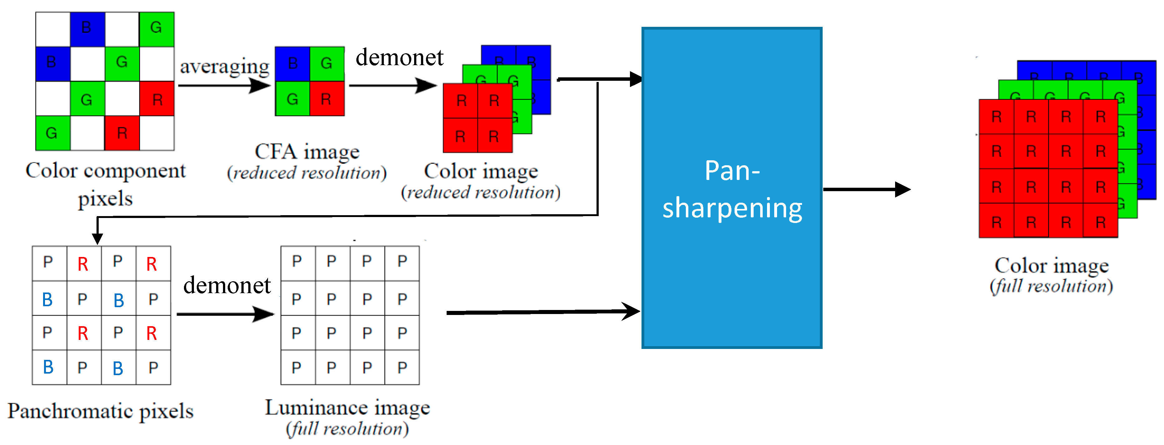
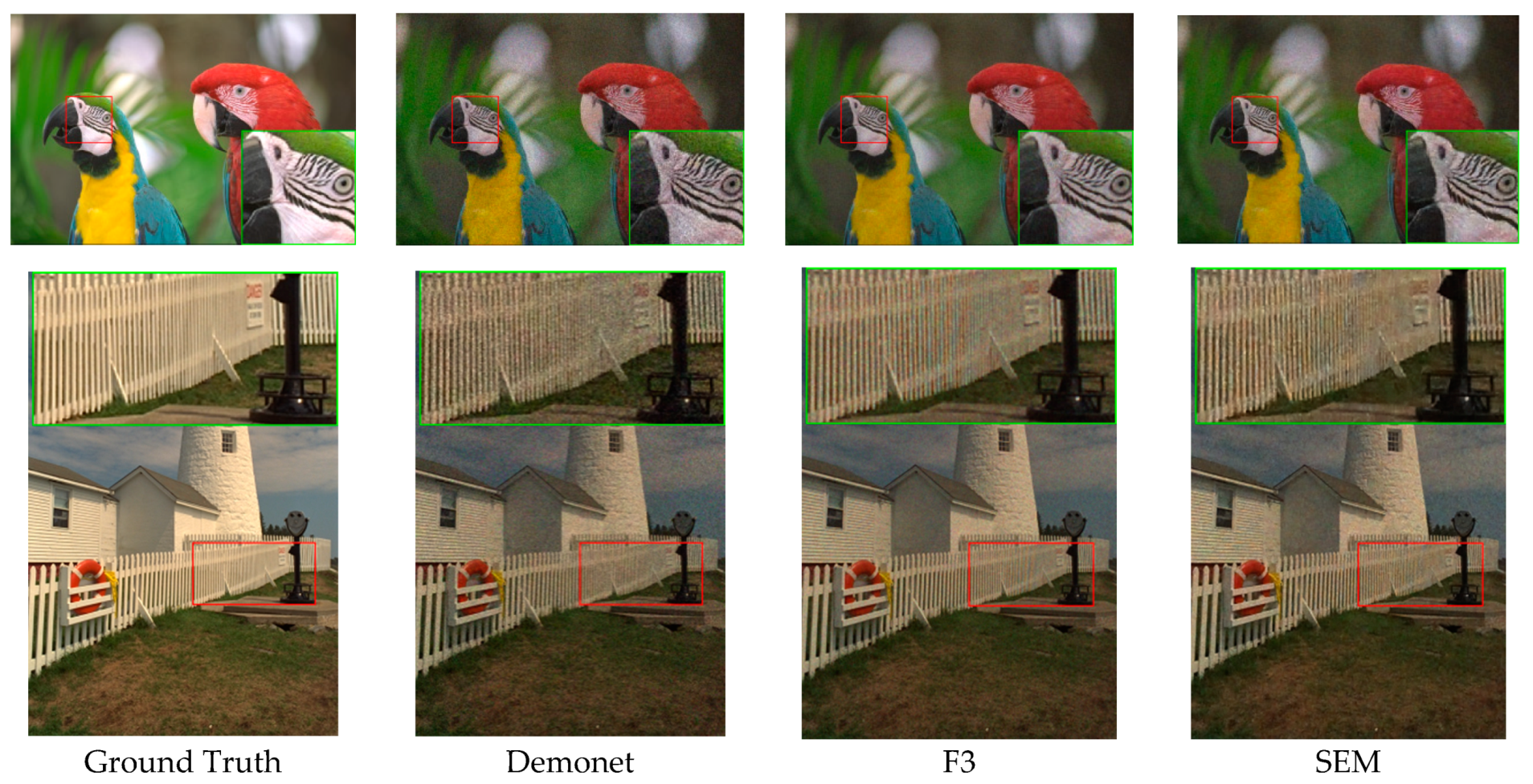
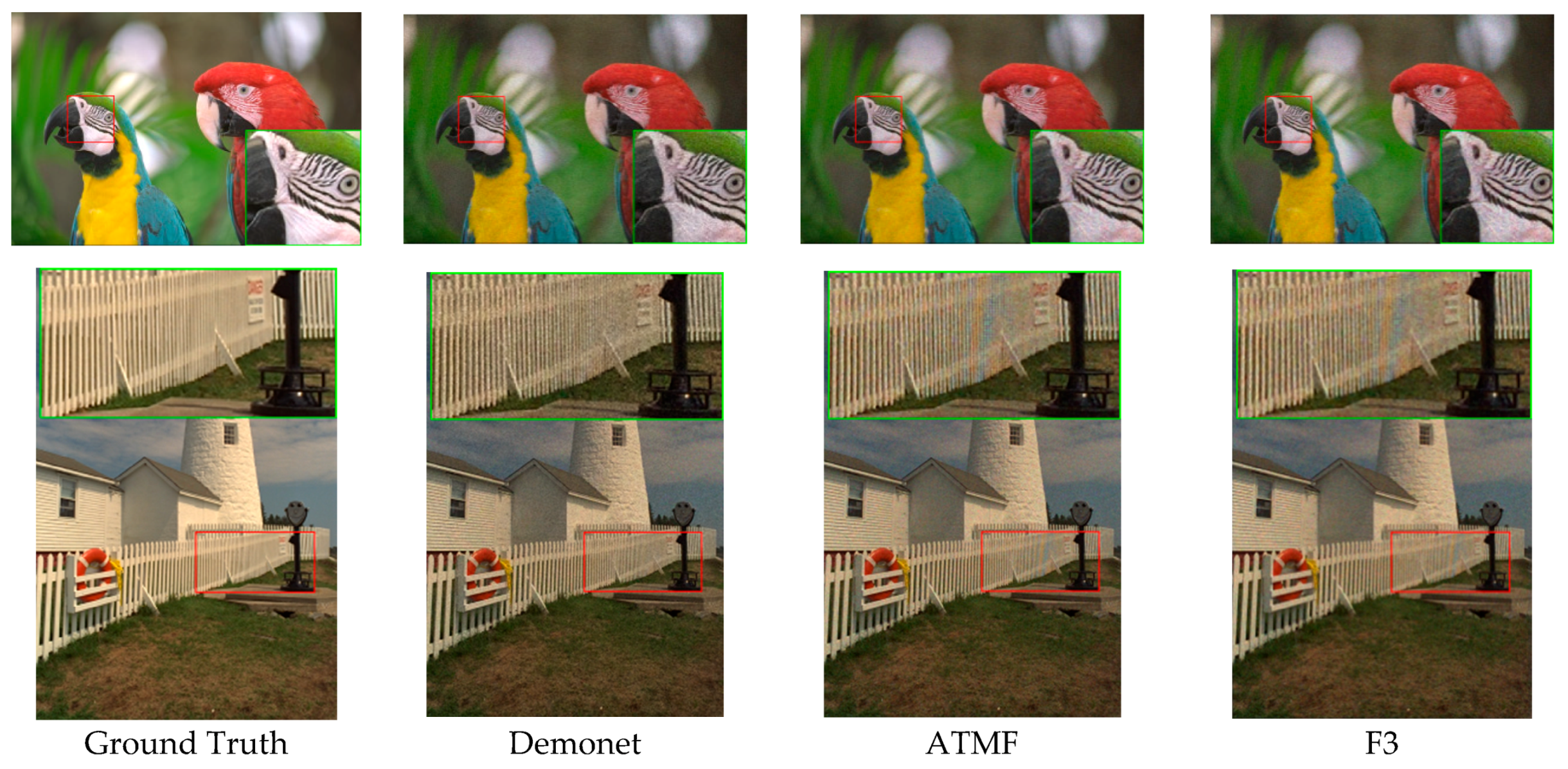
- Demosaicnet (Demonet): In [32], a feed-forward network architecture was proposed for demosaicing. There are D + 1 convolutional layers and each layer has W outputs and uses K × K size kernels. An initial model was trained using 1.3 million images from Imagenet and 1 million images from MirFlickr. Additionally, some challenging images were searched to further enhance the training model. Details can be found in [32];
- Fusion using three best (F3) [30]: The mean of pixels from demosaiced images of the three best individual methods were used;
- Bilinear: Bilinear interpolation is the simplest algorithm that uses the nearest neighbors for interpolation;
- Minimized-Laplacian Residual Interpolation (MLRI) [35]: This is a residual interpolation (RI)-based algorithm based on a minimized-Laplacian version;
- Adaptive Residual Interpolation (ARI) [36]: ARI adaptively combines RI and MLRI at each pixel, and adaptively selects a suitable iteration number for each pixel, instead of using a common iteration number for all of the pixels;
- Directional Difference Regression (DDR) [37]: DDR obtains the regression models using directional color differences of the training images. Once models are learned, they will be used for demosaicing.
2.2. Algorithms for Demosaicing CFA 2.0
3. Comparative Studies
3.1. Low Lighting Images and Denoising
3.2. Performance Metrics
3.3. CFA 1.0 Results
3.3.1. 10 dBs SNR Case
3.3.2. SNR at 20 dBs
3.4. CFA 2.0 Results
3.4.1. SNR at 10 dBs
3.4.2. SNR at 20 dBs
3.5. Best Against the Best Comparison Among the Two CFA Patterns
3.5.1. 10 dBs SNR
- In the no denoising case, CFA 2.0 is indeed better than CFA 1.0. For instance, the PSNR gain in Figure 34a is more than 4 dBs, which is significant;
- Denoising definitely improves the demosaicing performance, regardless of where the denoising is done. For CFA 1.0, the improvement over no denoising is about 4 dBs; for CFA 2.0, the improvement is more than 3 dBs in terms of PSNR. For other metrics in Figure 34b–e, we also observe big improvements;
- Denoising before demosaicing has a better performance than that of denoising after demosaicing. For CFA 1.0, the improvement is 1.1 dBs and, for CFA 2.0, the improvement is 2.1 dBs in PSNR.
3.5.2. 20 dBs SNR
- Denoising definitely helps the demosaicing performance, regardless of where the denoising is done. For CFA 1.0, the improvement is over 2 to 3.5 dBs; for CFA 2.0, the improvement is more than 1.1 to 4.8 dBs in terms of PSNR. There are also big improvements in other metrics (Figure 35b–e);
- Denoising before demosaicing has a better performance than that of denoising after demosaicing. For CFA 1.0, the improvement is 1.2 dBs and, for CFA 2.0, the improvement is close to 4 dBs in PSNR;
- Denoising helps the demosaicing performance more when the SNR is low. More than 4 dBs of gain in PSNR were observed after denoising in the 10 dBs SNR case;
3.5.3. Discussions
- Why denoising before demosaicing is better that that of after demosaicing:One intuitive explanation is that noise can be suppressed more effectively earlier rather than later. Once noise has propagated to subsequent steps in the processing pipeline, it is harder to suppress it because some steps in the demosaicing process may be nonlinear. For example, in deep learning approaches, some rectified linear units (ReLu) are inherently nonlinear. This intuition has been found to be valid in our past research on active noise suppression in noisy conditions, as well. For a NASA project on noise suppression in Space Station [66,67], we noticed that noise was suppressed more effectively near the source than farther away from the source, as there are more reflections in the far-field due to multipath propagations;
- Why CFA 2.0 is better than CFA 1.0 in low lighting conditions:We believe a concrete theory is needed to explain why CFA 2.0 has better performance than CFA 1.0 and this could be a good future research topic. The inventors of CFA 2.0 also did not provide a theory behind this. Intuitively, we agree with the inventors of CFA 2.0 that this must have something to do with the amount of white pixels in CFA 2.0. According to the inventors of CFA 2.0, more white pixels improve the sensitivity of the imager. We offer another analysis below.We use the bird image at 10 dBs condition (Image 1 in Figure 6 of our paper) as a case study. There is no denoising in the demosaicing process. Figure 36 below contains two histograms of the residual images (residual = reference − demosaiced) for CFAs 1.0 and 2.0. From this figure, it can be seen that the histogram of CFA 2.0 is centered near zero, whereas the histogram of CFA 1.0 is biased towards the right, meaning that CFA 2.0 is more accurate (close to the ground truth), because of its better light sensitivity, than CFA 1.0;
- Why denoising helps slightly more for 10 dBs case than the 20 dBs case:From Table 2 and 3, we noticed that the gap between denoising improvement in 10 dBs and 20 dBs is slim. However, we still noticed that denoising helps the demosaicing performance slightly more in the 10 dBs case than in the 20 dBs case. We do not have a concrete theory behind this. However, one intuitive explanation can be found using Figure 37, which is a hypothetical optimization problem. The x-axis shows the computational load and the y-axis shows the performance. This curve shows that, for the same amount of effort, the improvement in performance is higher in the early stage than the later. In other words, it is difficult to further improve once the system is already in good shape. In economics, there is a law of diminishing returns, which might be related to the case here.Although there is no physical law governing this behavior, we have seen similar observations in some engineering applications. For example, in a past paper on speech recognition [68] under noisy conditions, we noticed that the word recognition rate improves more when the SNR is low. See Table 1 in [68]. From that table, at 0 dB, the relative improvement is 140%, as compared to only 37% in the 6 dBs case. This implies that it may be easier to see improvements when a system starts from a poor condition.
4. Conclusions
Author Contributions
Funding
Conflicts of Interest
Appendix A. Performance Metrics of CFA 1.0 at 10 dBs. Three Cases: No Denoising, Denoising After Demosaicing, and Denoising Before Demosaicing

| Image | Metrics | Demonet | PCSD | DLMMSE | DDR | Bilinear | ARI | LDI | MHC | AP | AFD | LT | MLRI | ECC | SEM | F3 | ATMF | Best Score |
|---|---|---|---|---|---|---|---|---|---|---|---|---|---|---|---|---|---|---|
| Img1 | PSNR | 17.215 | 17.001 | 17.053 | 16.561 | 16.402 | 17.145 | 17.093 | 16.894 | 16.220 | 16.781 | 17.096 | 15.915 | 17.165 | 16.825 | 16.997 | 17.122 | 17.215 |
| Cielab | 11.325 | 12.046 | 11.517 | 12.420 | 14.085 | 12.691 | 11.722 | 12.652 | 12.702 | 12.035 | 11.688 | 13.485 | 12.019 | 11.656 | 11.393 | 11.369 | 11.325 | |
| SSIM | 0.218 | 0.195 | 0.195 | 0.203 | 0.210 | 0.250 | 0.202 | 0.194 | 0.186 | 0.188 | 0.200 | 0.204 | 0.212 | 0.299 | 0.332 | 0.235 | 0.332 | |
| HVS | 11.703 | 11.571 | 11.707 | 11.088 | 10.813 | 11.605 | 11.673 | 11.436 | 10.857 | 11.412 | 11.702 | 10.391 | 11.651 | 11.289 | 11.397 | 11.614 | 11.707 | |
| HVSm | 11.800 | 11.683 | 11.815 | 11.194 | 10.909 | 11.672 | 11.784 | 11.562 | 10.942 | 11.513 | 11.813 | 10.478 | 11.766 | 11.336 | 11.446 | 11.697 | 11.815 | |
| Img2 | PSNR | 15.498 | 15.435 | 15.460 | 15.475 | 15.335 | 16.148 | 15.456 | 15.316 | 15.399 | 15.406 | 15.467 | 15.016 | 15.484 | 16.624 | 15.977 | 15.638 | 16.624 |
| Cielab | 10.895 | 11.716 | 11.226 | 11.630 | 13.358 | 11.378 | 11.506 | 12.321 | 11.339 | 11.399 | 11.457 | 12.312 | 11.755 | 9.438 | 10.487 | 10.997 | 9.438 | |
| SSIM | 0.478 | 0.468 | 0.473 | 0.475 | 0.363 | 0.433 | 0.470 | 0.461 | 0.463 | 0.469 | 0.471 | 0.465 | 0.470 | 0.521 | 0.549 | 0.506 | 0.549 | |
| HVS | 10.912 | 10.782 | 10.848 | 10.829 | 10.661 | 11.502 | 10.815 | 10.661 | 10.807 | 10.774 | 10.836 | 10.343 | 10.802 | 12.009 | 11.301 | 10.966 | 12.009 | |
| HVSm | 11.007 | 10.889 | 10.952 | 10.942 | 10.805 | 11.619 | 10.923 | 10.778 | 10.911 | 10.877 | 10.943 | 10.443 | 10.911 | 12.112 | 11.386 | 11.059 | 12.112 | |
| Img3 | PSNR | 17.398 | 16.845 | 16.885 | 15.783 | 18.927 | 16.211 | 16.283 | 16.442 | 17.429 | 16.009 | 16.059 | 16.180 | 15.208 | 17.637 | 18.265 | 17.062 | 18.927 |
| Cielab | 11.456 | 12.404 | 11.797 | 13.825 | 12.296 | 14.240 | 12.958 | 13.431 | 11.122 | 13.199 | 13.264 | 13.360 | 14.979 | 10.698 | 10.233 | 11.625 | 10.233 | |
| SSIM | 0.354 | 0.330 | 0.331 | 0.329 | 0.345 | 0.354 | 0.331 | 0.330 | 0.325 | 0.318 | 0.329 | 0.331 | 0.324 | 0.424 | 0.453 | 0.373 | 0.453 | |
| HVS | 12.321 | 11.756 | 11.915 | 10.668 | 13.740 | 11.043 | 11.198 | 11.348 | 12.572 | 10.958 | 10.981 | 11.066 | 10.035 | 12.527 | 13.090 | 11.921 | 13.740 | |
| HVSm | 12.449 | 11.892 | 12.049 | 10.775 | 13.994 | 11.126 | 11.312 | 11.484 | 12.733 | 11.062 | 11.087 | 11.186 | 10.121 | 12.616 | 13.187 | 12.027 | 13.994 | |
| Img4 | PSNR | 14.876 | 14.625 | 14.851 | 14.755 | 14.579 | 11.843 | 14.864 | 13.712 | 14.725 | 14.752 | 14.877 | 14.841 | 14.492 | 14.789 | 15.209 | 14.992 | 15.209 |
| Cielab | 13.131 | 15.023 | 13.774 | 15.084 | 18.714 | 20.041 | 14.686 | 17.664 | 14.113 | 14.315 | 14.472 | 15.318 | 15.796 | 12.205 | 12.263 | 13.158 | 12.205 | |
| SSIM | 0.480 | 0.474 | 0.480 | 0.478 | 0.398 | 0.370 | 0.480 | 0.452 | 0.467 | 0.471 | 0.481 | 0.477 | 0.474 | 0.501 | 0.575 | 0.520 | 0.575 | |
| HVS | 10.583 | 10.140 | 10.471 | 10.257 | 9.929 | 7.168 | 10.384 | 9.131 | 10.381 | 10.372 | 10.425 | 10.336 | 9.916 | 10.347 | 10.606 | 10.456 | 10.606 | |
| HVSm | 10.871 | 10.437 | 10.775 | 10.569 | 10.300 | 7.323 | 10.696 | 9.387 | 10.684 | 10.675 | 10.735 | 10.661 | 10.201 | 10.598 | 10.840 | 10.722 | 10.871 | |
| Img5 | PSNR | 17.382 | 17.204 | 17.239 | 17.212 | 17.287 | 15.415 | 17.268 | 17.215 | 17.127 | 17.145 | 17.274 | 17.257 | 17.326 | 16.620 | 17.331 | 17.339 | 17.382 |
| Cielab | 8.939 | 9.561 | 9.155 | 9.621 | 11.231 | 12.521 | 9.467 | 10.171 | 9.284 | 9.364 | 9.404 | 9.762 | 9.880 | 9.584 | 9.106 | 9.112 | 8.939 | |
| SSIM | 0.269 | 0.261 | 0.263 | 0.265 | 0.237 | 0.259 | 0.265 | 0.258 | 0.255 | 0.257 | 0.265 | 0.263 | 0.266 | 0.311 | 0.354 | 0.293 | 0.354 | |
| HVS | 13.358 | 13.184 | 13.251 | 13.129 | 13.027 | 11.248 | 13.201 | 13.109 | 13.167 | 13.157 | 13.233 | 13.144 | 13.172 | 12.497 | 13.151 | 13.247 | 13.358 | |
| HVSm | 13.496 | 13.351 | 13.411 | 13.305 | 13.208 | 11.321 | 13.365 | 13.300 | 13.325 | 13.318 | 13.395 | 13.321 | 13.334 | 12.570 | 13.232 | 13.372 | 13.496 | |
| Img6 | PSNR | 18.292 | 17.986 | 18.080 | 18.097 | 18.342 | 19.737 | 18.111 | 17.636 | 17.762 | 17.983 | 18.127 | 17.484 | 17.558 | 18.612 | 18.811 | 18.382 | 19.737 |
| Cielab | 11.490 | 12.414 | 11.415 | 12.278 | 14.734 | 12.359 | 11.934 | 13.705 | 11.865 | 11.778 | 11.886 | 13.150 | 13.161 | 9.873 | 10.241 | 10.985 | 9.873 | |
| SSIM | 0.369 | 0.350 | 0.354 | 0.358 | 0.302 | 0.346 | 0.357 | 0.345 | 0.340 | 0.346 | 0.357 | 0.350 | 0.354 | 0.421 | 0.471 | 0.397 | 0.471 | |
| HVS | 14.075 | 13.832 | 14.032 | 13.903 | 13.985 | 15.598 | 13.943 | 13.396 | 13.744 | 13.952 | 14.005 | 13.244 | 13.262 | 14.308 | 14.477 | 14.138 | 15.598 | |
| HVSm | 14.308 | 14.103 | 14.300 | 14.196 | 14.317 | 15.923 | 14.214 | 13.668 | 13.994 | 14.219 | 14.276 | 13.482 | 13.489 | 14.497 | 14.661 | 14.362 | 15.923 | |
| Img7 | PSNR | 17.909 | 17.274 | 17.692 | 16.765 | 17.986 | 18.206 | 17.721 | 16.789 | 17.397 | 17.180 | 17.731 | 16.509 | 17.498 | 20.127 | 18.989 | 17.998 | 20.127 |
| Cielab | 10.019 | 11.190 | 10.154 | 11.900 | 12.891 | 11.504 | 10.642 | 12.553 | 10.556 | 10.922 | 10.551 | 12.479 | 11.462 | 7.059 | 8.757 | 9.843 | 7.059 | |
| SSIM | 0.341 | 0.322 | 0.326 | 0.324 | 0.263 | 0.312 | 0.327 | 0.314 | 0.312 | 0.319 | 0.327 | 0.320 | 0.328 | 0.410 | 0.444 | 0.367 | 0.444 | |
| HVS | 13.756 | 13.156 | 13.662 | 12.566 | 13.658 | 14.011 | 13.594 | 12.570 | 13.392 | 13.101 | 13.636 | 12.282 | 13.259 | 16.040 | 14.737 | 13.809 | 16.040 | |
| HVSm | 13.903 | 13.317 | 13.838 | 12.713 | 13.862 | 14.142 | 13.772 | 12.730 | 13.556 | 13.254 | 13.815 | 12.415 | 13.423 | 16.202 | 14.845 | 13.947 | 16.202 | |
| Img8 | PSNR | 16.828 | 17.117 | 17.175 | 16.844 | 17.035 | 17.155 | 16.885 | 16.825 | 15.952 | 16.700 | 16.879 | 16.563 | 16.337 | 17.183 | 17.255 | 17.135 | 17.255 |
| Cielab | 10.685 | 10.788 | 10.204 | 11.112 | 12.812 | 11.802 | 10.919 | 11.793 | 11.800 | 10.925 | 10.876 | 11.597 | 11.987 | 9.770 | 10.077 | 10.269 | 9.770 | |
| SSIM | 0.398 | 0.387 | 0.391 | 0.388 | 0.323 | 0.368 | 0.389 | 0.380 | 0.373 | 0.383 | 0.389 | 0.383 | 0.384 | 0.432 | 0.480 | 0.425 | 0.480 | |
| HVS | 11.911 | 12.205 | 12.361 | 11.960 | 12.055 | 12.222 | 11.997 | 11.921 | 11.094 | 11.849 | 12.014 | 11.640 | 11.376 | 12.250 | 12.257 | 12.177 | 12.361 | |
| HVSm | 12.048 | 12.382 | 12.534 | 12.133 | 12.278 | 12.375 | 12.163 | 12.108 | 11.224 | 12.005 | 12.178 | 11.803 | 11.523 | 12.367 | 12.374 | 12.318 | 12.534 | |
| Img9 | PSNR | 12.723 | 12.667 | 12.682 | 12.680 | 13.554 | 10.623 | 12.689 | 12.675 | 13.208 | 12.633 | 12.691 | 12.346 | 12.706 | 13.968 | 13.488 | 12.915 | 13.968 |
| Cielab | 11.754 | 12.117 | 11.819 | 12.065 | 12.191 | 15.968 | 11.986 | 12.477 | 11.114 | 11.970 | 11.954 | 12.646 | 12.220 | 9.859 | 10.682 | 11.468 | 9.859 | |
| SSIM | 0.277 | 0.270 | 0.272 | 0.271 | 0.236 | 0.239 | 0.273 | 0.268 | 0.269 | 0.269 | 0.273 | 0.269 | 0.273 | 0.303 | 0.331 | 0.295 | 0.331 | |
| HVS | 8.259 | 8.175 | 8.223 | 8.199 | 9.042 | 6.116 | 8.211 | 8.191 | 8.774 | 8.164 | 8.222 | 7.851 | 8.205 | 9.536 | 8.998 | 8.414 | 9.536 | |
| HVSm | 8.298 | 8.224 | 8.269 | 8.250 | 9.114 | 6.140 | 8.258 | 8.245 | 8.828 | 8.211 | 8.269 | 7.899 | 8.253 | 9.580 | 9.031 | 8.454 | 9.580 | |
| Img10 | PSNR | 16.970 | 16.781 | 16.546 | 16.651 | 16.317 | 17.822 | 16.853 | 16.243 | 15.820 | 16.656 | 16.712 | 16.691 | 16.888 | 17.492 | 17.140 | 16.974 | 17.822 |
| Cielab | 10.162 | 10.889 | 10.705 | 11.052 | 13.349 | 10.808 | 10.708 | 12.234 | 11.685 | 10.719 | 10.811 | 11.164 | 11.089 | 9.125 | 9.920 | 10.191 | 9.125 | |
| SSIM | 0.385 | 0.376 | 0.377 | 0.378 | 0.308 | 0.369 | 0.379 | 0.368 | 0.363 | 0.373 | 0.378 | 0.376 | 0.379 | 0.416 | 0.448 | 0.405 | 0.448 | |
| HVS | 13.160 | 12.985 | 12.744 | 12.783 | 12.354 | 14.003 | 13.002 | 12.358 | 11.987 | 12.877 | 12.881 | 12.819 | 12.991 | 13.583 | 13.211 | 13.103 | 14.003 | |
| HVSm | 13.324 | 13.181 | 12.918 | 12.973 | 12.573 | 14.212 | 13.194 | 12.544 | 12.136 | 13.061 | 13.066 | 13.011 | 13.182 | 13.733 | 13.346 | 13.264 | 14.212 | |
| Img11 | PSNR | 16.636 | 15.804 | 15.492 | 15.160 | 16.102 | 16.819 | 16.246 | 16.218 | 15.104 | 16.142 | 16.127 | 15.277 | 16.560 | 16.339 | 16.528 | 16.223 | 16.819 |
| Cielab | 11.650 | 13.110 | 13.154 | 14.039 | 14.262 | 12.528 | 12.284 | 13.021 | 13.846 | 12.272 | 12.416 | 13.990 | 12.274 | 11.517 | 11.513 | 12.044 | 11.513 | |
| SSIM | 0.384 | 0.362 | 0.361 | 0.360 | 0.321 | 0.358 | 0.371 | 0.364 | 0.347 | 0.359 | 0.370 | 0.360 | 0.374 | 0.419 | 0.478 | 0.411 | 0.478 | |
| HVS | 11.512 | 10.666 | 10.407 | 10.007 | 10.917 | 11.700 | 11.160 | 11.118 | 10.016 | 11.096 | 11.050 | 10.133 | 11.435 | 11.189 | 11.332 | 11.065 | 11.700 | |
| HVSm | 11.613 | 10.762 | 10.492 | 10.091 | 11.034 | 11.798 | 11.267 | 11.241 | 10.092 | 11.199 | 11.152 | 10.221 | 11.555 | 11.262 | 11.400 | 11.148 | 11.798 | |
| Img12 | PSNR | 16.766 | 16.013 | 16.686 | 16.228 | 16.626 | 16.893 | 16.688 | 15.488 | 15.545 | 15.890 | 16.699 | 15.931 | 16.062 | 16.457 | 16.831 | 16.554 | 16.893 |
| Cielab | 10.962 | 12.348 | 11.000 | 12.166 | 13.334 | 11.919 | 11.376 | 13.723 | 12.642 | 12.229 | 11.306 | 12.643 | 12.528 | 11.005 | 10.717 | 11.172 | 10.717 | |
| SSIM | 0.451 | 0.429 | 0.439 | 0.431 | 0.377 | 0.427 | 0.441 | 0.420 | 0.414 | 0.422 | 0.442 | 0.429 | 0.434 | 0.502 | 0.543 | 0.479 | 0.543 | |
| HVS | 12.210 | 11.383 | 12.167 | 11.615 | 12.070 | 12.360 | 12.111 | 10.863 | 10.965 | 11.321 | 12.129 | 11.316 | 11.439 | 11.851 | 12.208 | 11.921 | 12.360 | |
| HVSm | 12.346 | 11.516 | 12.319 | 11.758 | 12.284 | 12.519 | 12.267 | 10.991 | 11.082 | 11.446 | 12.283 | 11.451 | 11.574 | 11.959 | 12.323 | 12.045 | 12.519 | |
| Average | PSNR | 16.541 | 16.229 | 16.320 | 16.018 | 16.541 | 16.168 | 16.347 | 15.954 | 15.974 | 16.106 | 16.312 | 15.834 | 16.107 | 16.889 | 16.902 | 16.528 | 16.902 |
| Cielab | 11.039 | 11.967 | 11.327 | 12.266 | 13.605 | 13.147 | 11.682 | 12.979 | 11.839 | 11.761 | 11.674 | 12.659 | 12.429 | 10.149 | 10.449 | 11.019 | 10.149 | |
| SSIM | 0.367 | 0.352 | 0.355 | 0.355 | 0.307 | 0.340 | 0.357 | 0.346 | 0.343 | 0.348 | 0.357 | 0.352 | 0.356 | 0.413 | 0.455 | 0.392 | 0.455 | |
| HVS | 11.980 | 11.653 | 11.816 | 11.417 | 11.854 | 11.548 | 11.774 | 11.342 | 11.480 | 11.586 | 11.759 | 11.214 | 11.462 | 12.285 | 12.230 | 11.903 | 12.285 | |
| HVSm | 12.122 | 11.811 | 11.973 | 11.575 | 12.057 | 11.681 | 11.935 | 11.503 | 11.626 | 11.737 | 11.918 | 11.364 | 11.611 | 12.403 | 12.339 | 12.034 | 12.403 |
| Image | Metrics | Demonet | PCSD | DLMMSE | DDR | Bilinear | ARI | LDI | MHC | AP | AFD | LT | MLRI | ECC | SEM | F3 | ATMF | Best Score |
|---|---|---|---|---|---|---|---|---|---|---|---|---|---|---|---|---|---|---|
| Img1 | PSNR | 18.633 | 18.817 | 19.054 | 19.121 | 20.651 | 19.127 | 18.543 | 18.134 | 22.081 | 19.195 | 18.733 | 18.297 | 18.488 | 20.280 | 20.221 | 19.785 | 22.081 |
| Cielab | 9.110 | 9.371 | 8.852 | 8.836 | 7.847 | 9.199 | 9.418 | 10.108 | 6.687 | 8.883 | 9.233 | 9.708 | 9.535 | 7.934 | 7.604 | 7.903 | 6.687 | |
| SSIM | 0.395 | 0.366 | 0.384 | 0.366 | 0.337 | 0.349 | 0.362 | 0.339 | 0.396 | 0.377 | 0.367 | 0.355 | 0.352 | 0.409 | 0.430 | 0.433 | 0.433 | |
| HVS | 12.926 | 13.118 | 13.423 | 13.436 | 14.956 | 13.505 | 12.893 | 12.464 | 16.478 | 13.522 | 13.096 | 12.627 | 12.814 | 14.723 | 14.597 | 14.143 | 16.478 | |
| HVSm | 12.979 | 13.180 | 13.484 | 13.506 | 15.094 | 13.580 | 12.953 | 12.527 | 16.595 | 13.586 | 13.157 | 12.688 | 12.878 | 14.797 | 14.672 | 14.208 | 16.595 | |
| Img2 | PSNR | 18.084 | 18.578 | 18.964 | 18.826 | 19.949 | 20.205 | 18.463 | 16.879 | 18.991 | 18.301 | 18.574 | 16.700 | 18.009 | 20.685 | 19.569 | 19.154 | 20.685 |
| Cielab | 7.843 | 8.002 | 7.313 | 7.764 | 7.401 | 7.121 | 7.894 | 9.778 | 7.396 | 8.003 | 7.787 | 9.712 | 8.428 | 5.782 | 6.566 | 6.839 | 5.782 | |
| SSIM | 0.513 | 0.513 | 0.526 | 0.515 | 0.376 | 0.408 | 0.501 | 0.485 | 0.520 | 0.520 | 0.506 | 0.484 | 0.483 | 0.464 | 0.482 | 0.531 | 0.531 | |
| HVS | 13.424 | 13.843 | 14.276 | 14.127 | 15.367 | 15.675 | 13.770 | 12.161 | 14.284 | 13.546 | 13.892 | 11.981 | 13.308 | 16.177 | 15.019 | 14.486 | 16.177 | |
| HVSm | 13.550 | 14.000 | 14.438 | 14.293 | 15.732 | 15.975 | 13.929 | 12.281 | 14.452 | 13.688 | 14.050 | 12.090 | 13.454 | 16.435 | 15.223 | 14.647 | 16.435 | |
| Img3 | PSNR | 21.401 | 21.132 | 20.615 | 19.756 | 22.395 | 19.260 | 19.814 | 20.237 | 23.351 | 20.167 | 19.448 | 20.109 | 18.111 | 22.521 | 22.149 | 21.480 | 23.351 |
| Cielab | 7.137 | 7.708 | 7.693 | 8.575 | 7.193 | 9.639 | 8.446 | 8.479 | 6.242 | 8.247 | 8.767 | 8.313 | 10.186 | 6.403 | 6.441 | 6.721 | 6.242 | |
| SSIM | 0.522 | 0.501 | 0.511 | 0.488 | 0.454 | 0.450 | 0.488 | 0.476 | 0.521 | 0.500 | 0.488 | 0.481 | 0.459 | 0.523 | 0.539 | 0.551 | 0.551 | |
| HVS | 16.069 | 15.690 | 15.349 | 14.450 | 16.987 | 14.019 | 14.519 | 14.896 | 18.009 | 14.837 | 14.178 | 14.797 | 12.830 | 17.412 | 16.952 | 16.217 | 18.009 | |
| HVSm | 16.221 | 15.849 | 15.488 | 14.579 | 17.304 | 14.154 | 14.648 | 15.052 | 18.264 | 14.966 | 14.296 | 14.938 | 12.927 | 17.627 | 17.145 | 16.371 | 18.264 | |
| Img4 | PSNR | 17.287 | 15.222 | 15.440 | 15.066 | 16.574 | 12.411 | 16.640 | 14.179 | 16.889 | 16.391 | 16.788 | 15.285 | 14.716 | 17.130 | 17.371 | 17.094 | 17.371 |
| Cielab | 10.375 | 20.858 | 20.576 | 14.186 | 14.899 | 18.289 | 12.423 | 16.290 | 11.645 | 12.260 | 12.124 | 14.190 | 21.141 | 9.366 | 9.550 | 9.735 | 9.366 | |
| SSIM | 0.569 | 0.487 | 0.495 | 0.525 | 0.446 | 0.380 | 0.547 | 0.493 | 0.541 | 0.541 | 0.552 | 0.523 | 0.463 | 0.601 | 0.632 | 0.626 | 0.632 | |
| HVS | 12.924 | 11.453 | 11.767 | 10.397 | 11.849 | 7.732 | 12.031 | 9.493 | 12.457 | 11.869 | 12.212 | 10.620 | 10.840 | 12.570 | 12.772 | 12.488 | 12.924 | |
| HVSm | 13.303 | 11.938 | 12.275 | 10.666 | 12.381 | 7.903 | 12.406 | 9.736 | 12.855 | 12.220 | 12.595 | 10.911 | 11.269 | 12.883 | 13.106 | 12.793 | 13.303 | |
| Img5 | PSNR | 23.498 | 22.842 | 22.671 | 22.971 | 21.832 | 18.074 | 23.198 | 20.259 | 19.933 | 22.018 | 23.299 | 23.446 | 23.001 | 19.360 | 21.712 | 22.137 | 23.498 |
| Cielab | 4.370 | 5.129 | 4.995 | 5.140 | 6.052 | 8.551 | 4.944 | 6.834 | 6.703 | 5.470 | 4.874 | 4.979 | 5.199 | 6.843 | 5.236 | 5.020 | 4.370 | |
| SSIM | 0.360 | 0.351 | 0.359 | 0.345 | 0.284 | 0.285 | 0.346 | 0.330 | 0.345 | 0.353 | 0.348 | 0.341 | 0.333 | 0.326 | 0.355 | 0.375 | 0.375 | |
| HVS | 19.209 | 18.518 | 18.369 | 18.550 | 17.365 | 13.874 | 18.828 | 15.907 | 15.634 | 17.658 | 18.957 | 18.986 | 18.580 | 15.202 | 17.514 | 17.914 | 19.209 | |
| HVSm | 19.430 | 18.752 | 18.572 | 18.800 | 17.678 | 13.981 | 19.082 | 16.068 | 15.755 | 17.844 | 19.210 | 19.271 | 18.845 | 15.303 | 17.687 | 18.081 | 19.430 | |
| Img6 | PSNR | 22.626 | 21.705 | 22.785 | 21.617 | 23.185 | 22.764 | 21.438 | 20.442 | 19.337 | 23.257 | 21.922 | 20.440 | 21.624 | 22.592 | 23.193 | 22.543 | 23.257 |
| Cielab | 6.842 | 8.093 | 6.795 | 8.070 | 7.852 | 8.105 | 7.893 | 9.243 | 9.293 | 6.971 | 7.590 | 8.857 | 8.099 | 6.359 | 6.055 | 6.369 | 6.055 | |
| SSIM | 0.428 | 0.438 | 0.451 | 0.435 | 0.347 | 0.349 | 0.428 | 0.417 | 0.402 | 0.447 | 0.433 | 0.416 | 0.410 | 0.359 | 0.417 | 0.450 | 0.451 | |
| HVS | 18.168 | 17.185 | 18.365 | 17.120 | 18.626 | 18.549 | 16.974 | 15.933 | 14.905 | 18.753 | 17.498 | 15.997 | 17.164 | 18.288 | 19.004 | 18.163 | 19.004 | |
| HVSm | 18.561 | 17.542 | 18.807 | 17.486 | 19.371 | 19.160 | 17.321 | 16.238 | 15.125 | 19.244 | 17.880 | 16.277 | 17.539 | 18.777 | 19.534 | 18.568 | 19.534 | |
| Img7 | PSNR | 25.621 | 25.076 | 26.870 | 24.030 | 24.849 | 23.871 | 25.453 | 21.866 | 25.894 | 26.066 | 25.881 | 24.384 | 24.482 | 26.868 | 26.528 | 26.799 | 26.870 |
| Cielab | 4.328 | 5.207 | 4.307 | 5.794 | 5.976 | 6.176 | 5.088 | 7.102 | 4.781 | 4.818 | 4.898 | 5.731 | 5.670 | 3.494 | 3.767 | 3.758 | 3.494 | |
| SSIM | 0.450 | 0.440 | 0.459 | 0.429 | 0.312 | 0.328 | 0.427 | 0.402 | 0.443 | 0.452 | 0.433 | 0.421 | 0.407 | 0.406 | 0.436 | 0.479 | 0.479 | |
| HVS | 21.236 | 20.606 | 22.440 | 19.464 | 20.143 | 19.648 | 20.943 | 17.341 | 21.341 | 21.454 | 21.413 | 19.803 | 19.915 | 23.059 | 22.546 | 22.631 | 23.059 | |
| HVSm | 21.677 | 21.047 | 23.076 | 19.831 | 20.769 | 20.082 | 21.440 | 17.600 | 21.853 | 21.974 | 21.954 | 20.214 | 20.340 | 23.842 | 23.195 | 23.222 | 23.842 | |
| Img8 | PSNR | 22.581 | 21.262 | 21.668 | 21.481 | 22.362 | 21.289 | 22.441 | 19.943 | 22.151 | 21.202 | 22.109 | 21.087 | 21.980 | 23.574 | 23.136 | 22.460 | 23.574 |
| Cielab | 5.500 | 6.804 | 6.202 | 6.674 | 6.697 | 7.241 | 6.023 | 8.004 | 6.097 | 6.705 | 6.162 | 6.931 | 6.439 | 4.790 | 5.067 | 5.351 | 4.790 | |
| SSIM | 0.480 | 0.480 | 0.491 | 0.472 | 0.380 | 0.396 | 0.476 | 0.455 | 0.487 | 0.484 | 0.477 | 0.463 | 0.455 | 0.440 | 0.478 | 0.513 | 0.513 | |
| HVS | 17.470 | 16.062 | 16.585 | 16.399 | 17.306 | 16.345 | 17.354 | 14.844 | 17.055 | 16.060 | 17.054 | 15.994 | 16.889 | 18.733 | 18.245 | 17.412 | 18.733 | |
| HVSm | 17.741 | 16.304 | 16.839 | 16.659 | 17.882 | 16.667 | 17.678 | 15.060 | 17.346 | 16.294 | 17.350 | 16.240 | 17.190 | 19.115 | 18.624 | 17.687 | 19.115 | |
| Img9 | PSNR | 18.522 | 16.339 | 18.439 | 17.025 | 18.982 | 11.088 | 19.316 | 15.181 | 17.822 | 17.544 | 18.475 | 16.823 | 15.973 | 18.082 | 18.712 | 18.476 | 19.316 |
| Cielab | 5.907 | 7.790 | 6.100 | 7.210 | 6.388 | 14.595 | 5.721 | 9.001 | 6.580 | 6.800 | 6.172 | 7.397 | 8.106 | 6.160 | 5.758 | 5.837 | 5.721 | |
| SSIM | 0.322 | 0.314 | 0.326 | 0.315 | 0.262 | 0.224 | 0.320 | 0.304 | 0.320 | 0.321 | 0.320 | 0.311 | 0.300 | 0.289 | 0.311 | 0.333 | 0.333 | |
| HVS | 14.046 | 11.775 | 13.925 | 12.489 | 14.443 | 6.577 | 14.787 | 10.646 | 13.288 | 12.985 | 13.962 | 12.284 | 11.442 | 13.643 | 14.265 | 13.990 | 14.787 | |
| HVSm | 14.107 | 11.826 | 13.995 | 12.548 | 14.602 | 6.601 | 14.878 | 10.693 | 13.353 | 13.046 | 14.036 | 12.343 | 11.493 | 13.701 | 14.340 | 14.053 | 14.878 | |
| Img10 | PSNR | 19.388 | 19.724 | 19.683 | 18.734 | 19.942 | 20.919 | 19.227 | 17.060 | 17.770 | 19.758 | 19.135 | 17.302 | 19.047 | 20.644 | 20.218 | 19.624 | 20.919 |
| Cielab | 7.405 | 7.689 | 7.384 | 8.480 | 7.953 | 7.283 | 7.938 | 10.451 | 9.152 | 7.531 | 7.980 | 9.863 | 8.244 | 6.260 | 6.609 | 7.048 | 6.260 | |
| SSIM | 0.429 | 0.435 | 0.439 | 0.422 | 0.340 | 0.372 | 0.423 | 0.402 | 0.417 | 0.439 | 0.425 | 0.404 | 0.411 | 0.397 | 0.422 | 0.445 | 0.445 | |
| HVS | 15.439 | 15.778 | 15.725 | 14.738 | 15.923 | 17.085 | 15.237 | 13.078 | 13.767 | 15.775 | 15.173 | 13.325 | 15.071 | 16.723 | 16.342 | 15.665 | 17.085 | |
| HVSm | 15.641 | 16.029 | 15.959 | 14.939 | 16.338 | 17.503 | 15.466 | 13.233 | 13.934 | 16.016 | 15.394 | 13.481 | 15.295 | 17.021 | 16.622 | 15.887 | 17.503 | |
| Img11 | PSNR | 19.170 | 19.845 | 19.225 | 19.189 | 20.750 | 21.170 | 19.868 | 19.245 | 19.499 | 18.755 | 20.116 | 18.605 | 19.977 | 18.467 | 19.534 | 19.492 | 21.170 |
| Cielab | 8.290 | 8.096 | 8.268 | 8.550 | 7.678 | 7.440 | 7.867 | 8.797 | 8.158 | 8.863 | 7.665 | 9.128 | 7.961 | 8.788 | 7.714 | 7.750 | 7.440 | |
| SSIM | 0.408 | 0.440 | 0.437 | 0.426 | 0.360 | 0.360 | 0.434 | 0.434 | 0.434 | 0.429 | 0.437 | 0.419 | 0.416 | 0.323 | 0.401 | 0.448 | 0.448 | |
| HVS | 13.985 | 14.572 | 14.053 | 13.981 | 15.593 | 16.126 | 14.689 | 14.033 | 14.310 | 13.533 | 14.956 | 13.405 | 14.794 | 13.348 | 14.429 | 14.342 | 16.126 | |
| HVSm | 14.110 | 14.723 | 14.183 | 14.116 | 15.855 | 16.380 | 14.846 | 14.182 | 14.448 | 13.651 | 15.120 | 13.526 | 14.963 | 13.474 | 14.575 | 14.474 | 16.380 | |
| Img12 | PSNR | 18.298 | 17.711 | 17.768 | 17.574 | 16.583 | 20.013 | 17.849 | 16.304 | 17.470 | 17.857 | 17.903 | 17.930 | 17.782 | 17.146 | 17.569 | 17.758 | 20.013 |
| Cielab | 8.797 | 9.560 | 9.302 | 9.765 | 11.602 | 7.713 | 9.468 | 11.548 | 9.669 | 9.374 | 9.293 | 9.390 | 9.550 | 10.357 | 9.597 | 9.190 | 7.713 | |
| SSIM | 0.520 | 0.514 | 0.524 | 0.503 | 0.397 | 0.451 | 0.511 | 0.481 | 0.510 | 0.520 | 0.513 | 0.507 | 0.492 | 0.461 | 0.498 | 0.533 | 0.533 | |
| HVS | 13.708 | 13.011 | 13.147 | 12.907 | 12.088 | 15.663 | 13.224 | 11.641 | 12.806 | 13.211 | 13.266 | 13.291 | 13.160 | 12.633 | 13.064 | 13.178 | 15.663 | |
| HVSm | 13.859 | 13.161 | 13.293 | 13.052 | 12.272 | 15.997 | 13.381 | 11.761 | 12.949 | 13.360 | 13.421 | 13.451 | 13.319 | 12.762 | 13.208 | 13.316 | 15.997 | |
| Average | PSNR | 20.426 | 19.854 | 20.265 | 19.616 | 20.671 | 19.183 | 20.188 | 18.311 | 20.099 | 20.043 | 20.199 | 19.201 | 19.432 | 20.613 | 20.826 | 20.567 | 20.826 |
| Cielab | 7.159 | 8.692 | 8.149 | 8.254 | 8.128 | 9.279 | 7.760 | 9.636 | 7.700 | 7.827 | 7.712 | 8.683 | 9.047 | 6.878 | 6.664 | 6.793 | 6.664 | |
| SSIM | 0.450 | 0.440 | 0.450 | 0.437 | 0.358 | 0.363 | 0.439 | 0.418 | 0.445 | 0.448 | 0.442 | 0.427 | 0.415 | 0.416 | 0.450 | 0.476 | 0.476 | |
| HVS | 15.717 | 15.134 | 15.619 | 14.838 | 15.887 | 14.567 | 15.438 | 13.536 | 15.361 | 15.267 | 15.471 | 14.426 | 14.734 | 16.043 | 16.229 | 15.886 | 16.229 | |
| HVSm | 15.932 | 15.363 | 15.867 | 15.039 | 16.273 | 14.832 | 15.669 | 13.703 | 15.578 | 15.491 | 15.705 | 14.619 | 14.959 | 16.311 | 16.494 | 16.109 | 16.494 |
| Image | Metrics | Demonet | PCSD | DLMMSE | DDR | Bilinear | ARI | LDI | MHC | AP | AFD | LT | MLRI | ECC | SEM | F3 | ATMF | Best Score |
|---|---|---|---|---|---|---|---|---|---|---|---|---|---|---|---|---|---|---|
| Img1 | PSNR | 19.813 | 19.772 | 19.807 | 19.779 | 20.502 | 19.807 | 19.813 | 19.833 | 20.624 | 19.756 | 21.410 | 19.817 | 19.809 | 21.545 | 20.800 | 19.962 | 21.545 |
| Cielab | 7.897 | 7.960 | 7.839 | 7.827 | 7.997 | 7.877 | 7.824 | 7.852 | 7.803 | 7.891 | 10.137 | 7.830 | 7.846 | 7.352 | 8.123 | 7.775 | 7.352 | |
| SSIM | 0.402 | 0.397 | 0.406 | 0.407 | 0.401 | 0.400 | 0.406 | 0.408 | 0.421 | 0.403 | 0.211 | 0.408 | 0.402 | 0.413 | 0.361 | 0.415 | 0.421 | |
| HVS | 14.099 | 14.097 | 14.158 | 14.126 | 16.141 | 14.171 | 14.162 | 14.181 | 16.275 | 14.086 | 14.270 | 14.170 | 14.163 | 16.037 | 14.948 | 14.367 | 16.275 | |
| HVSm | 14.161 | 14.163 | 14.223 | 14.189 | 16.279 | 14.239 | 14.228 | 14.244 | 16.375 | 14.151 | 14.363 | 14.235 | 14.230 | 16.126 | 15.021 | 14.432 | 16.375 | |
| Img2 | PSNR | 21.603 | 21.533 | 21.576 | 21.568 | 20.469 | 21.484 | 21.526 | 21.475 | 21.078 | 21.485 | 21.323 | 21.547 | 21.544 | 21.765 | 21.472 | 21.555 | 21.765 |
| Cielab | 5.413 | 5.553 | 5.387 | 5.453 | 7.174 | 5.565 | 5.463 | 5.674 | 6.079 | 5.466 | 8.720 | 5.474 | 5.480 | 5.217 | 6.190 | 5.496 | 5.217 | |
| SSIM | 0.542 | 0.539 | 0.544 | 0.543 | 0.387 | 0.520 | 0.536 | 0.532 | 0.516 | 0.541 | 0.453 | 0.537 | 0.538 | 0.512 | 0.531 | 0.542 | 0.544 | |
| HVS | 16.917 | 16.838 | 16.914 | 16.923 | 15.266 | 16.887 | 16.887 | 16.880 | 15.723 | 16.789 | 16.046 | 16.889 | 16.889 | 17.022 | 16.365 | 16.814 | 17.022 | |
| HVSm | 17.169 | 17.100 | 17.176 | 17.189 | 15.597 | 17.166 | 17.158 | 17.163 | 15.938 | 17.046 | 16.309 | 17.153 | 17.153 | 17.296 | 16.591 | 17.068 | 17.296 | |
| Img3 | PSNR | 24.197 | 24.097 | 24.151 | 24.170 | 24.854 | 24.106 | 24.161 | 24.210 | 25.504 | 24.064 | 24.298 | 24.156 | 24.152 | 22.627 | 26.060 | 24.653 | 26.060 |
| Cielab | 5.707 | 5.835 | 5.663 | 5.661 | 9.136 | 5.905 | 5.674 | 5.673 | 8.822 | 5.725 | 9.903 | 5.704 | 5.694 | 6.494 | 7.455 | 5.740 | 5.661 | |
| SSIM | 0.539 | 0.535 | 0.540 | 0.544 | 0.500 | 0.532 | 0.541 | 0.542 | 0.534 | 0.536 | 0.465 | 0.540 | 0.539 | 0.534 | 0.545 | 0.549 | 0.549 | |
| HVS | 19.060 | 18.942 | 19.112 | 19.130 | 15.022 | 19.114 | 19.109 | 19.164 | 15.233 | 18.940 | 15.137 | 19.116 | 19.124 | 17.528 | 16.449 | 18.436 | 19.164 | |
| HVSm | 19.303 | 19.196 | 19.370 | 19.388 | 15.190 | 19.380 | 19.368 | 19.423 | 15.349 | 19.190 | 15.283 | 19.375 | 19.384 | 17.708 | 16.591 | 18.652 | 19.423 | |
| Img4 | PSNR | 17.519 | 17.476 | 17.529 | 17.514 | 16.411 | 17.869 | 17.534 | 17.375 | 16.824 | 17.412 | 16.888 | 17.507 | 17.555 | 16.152 | 17.614 | 17.565 | 17.869 |
| Cielab | 9.608 | 11.395 | 10.493 | 11.512 | 15.537 | 11.890 | 11.265 | 12.869 | 11.396 | 10.973 | 12.250 | 11.709 | 11.743 | 10.728 | 9.184 | 10.620 | 9.184 | |
| SSIM | 0.542 | 0.543 | 0.547 | 0.547 | 0.443 | 0.529 | 0.546 | 0.533 | 0.526 | 0.540 | 0.528 | 0.544 | 0.546 | 0.543 | 0.611 | 0.560 | 0.611 | |
| HVS | 13.364 | 13.065 | 13.228 | 13.073 | 11.151 | 13.357 | 13.111 | 12.904 | 11.809 | 13.096 | 12.436 | 13.048 | 13.050 | 11.694 | 12.821 | 13.107 | 13.364 | |
| HVSm | 13.815 | 13.543 | 13.695 | 13.557 | 11.597 | 13.844 | 13.590 | 13.425 | 12.159 | 13.557 | 12.861 | 13.538 | 13.532 | 11.993 | 13.157 | 13.550 | 13.844 | |
| Img5 | PSNR | 23.825 | 23.755 | 23.803 | 23.772 | 22.393 | 23.760 | 23.801 | 23.784 | 22.800 | 23.668 | 25.101 | 23.794 | 23.786 | 21.219 | 24.103 | 23.869 | 25.101 |
| Cielab | 4.670 | 4.770 | 4.688 | 4.702 | 7.066 | 4.758 | 4.671 | 4.810 | 6.680 | 4.757 | 6.773 | 4.701 | 4.711 | 6.000 | 5.683 | 4.712 | 4.670 | |
| SSIM | 0.370 | 0.369 | 0.376 | 0.370 | 0.298 | 0.356 | 0.372 | 0.371 | 0.351 | 0.371 | 0.321 | 0.365 | 0.365 | 0.348 | 0.371 | 0.373 | 0.376 | |
| HVS | 19.914 | 19.897 | 19.933 | 19.882 | 17.209 | 19.914 | 19.929 | 19.936 | 17.539 | 19.773 | 18.713 | 19.925 | 19.923 | 17.308 | 18.858 | 19.745 | 19.936 | |
| HVSm | 20.157 | 20.150 | 20.181 | 20.132 | 17.464 | 20.177 | 20.182 | 20.196 | 17.706 | 20.020 | 18.947 | 20.177 | 20.175 | 17.446 | 19.053 | 19.980 | 20.196 | |
| Img6 | PSNR | 20.465 | 20.420 | 20.460 | 20.468 | 23.033 | 20.406 | 20.448 | 20.460 | 23.928 | 20.405 | 23.886 | 20.443 | 20.443 | 22.027 | 23.006 | 21.031 | 23.928 |
| Cielab | 7.825 | 7.911 | 7.701 | 7.780 | 10.465 | 7.899 | 7.733 | 7.888 | 9.808 | 7.775 | 7.537 | 7.793 | 7.787 | 6.581 | 7.738 | 7.574 | 6.581 | |
| SSIM | 0.404 | 0.403 | 0.407 | 0.406 | 0.333 | 0.386 | 0.404 | 0.405 | 0.411 | 0.405 | 0.358 | 0.399 | 0.399 | 0.393 | 0.414 | 0.408 | 0.414 | |
| HVS | 16.217 | 16.161 | 16.225 | 16.210 | 17.054 | 16.229 | 16.205 | 16.262 | 17.590 | 16.162 | 17.583 | 16.226 | 16.229 | 17.808 | 17.288 | 16.470 | 17.808 | |
| HVSm | 16.463 | 16.415 | 16.481 | 16.473 | 17.516 | 16.496 | 16.463 | 16.522 | 17.947 | 16.417 | 17.993 | 16.480 | 16.485 | 18.161 | 17.606 | 16.737 | 18.161 | |
| Img7 | PSNR | 27.428 | 27.295 | 27.401 | 27.329 | 22.517 | 27.308 | 27.371 | 27.279 | 22.846 | 27.238 | 21.820 | 27.373 | 27.375 | 25.762 | 24.515 | 27.736 | 27.736 |
| Cielab | 4.439 | 4.537 | 4.406 | 4.451 | 13.519 | 4.527 | 4.401 | 4.458 | 13.236 | 4.497 | 14.096 | 4.472 | 4.465 | 4.802 | 10.064 | 5.395 | 4.401 | |
| SSIM | 0.471 | 0.470 | 0.475 | 0.475 | 0.360 | 0.468 | 0.469 | 0.465 | 0.449 | 0.471 | 0.314 | 0.474 | 0.473 | 0.461 | 0.454 | 0.478 | 0.478 | |
| HVS | 23.212 | 23.153 | 23.303 | 23.213 | 15.946 | 23.230 | 23.302 | 23.288 | 16.176 | 23.083 | 16.633 | 23.243 | 23.234 | 21.429 | 18.498 | 22.114 | 23.303 | |
| HVSm | 23.858 | 23.808 | 23.972 | 23.881 | 16.131 | 23.904 | 23.986 | 24.008 | 16.311 | 23.722 | 16.827 | 23.909 | 23.899 | 21.866 | 18.713 | 22.607 | 24.008 | |
| Img8 | PSNR | 22.125 | 22.057 | 22.115 | 22.092 | 23.681 | 22.056 | 22.089 | 22.003 | 25.340 | 22.023 | 24.412 | 22.096 | 22.093 | 21.109 | 24.822 | 22.602 | 25.340 |
| Cielab | 5.693 | 5.795 | 5.642 | 5.688 | 9.145 | 5.858 | 5.681 | 5.930 | 8.464 | 5.715 | 5.490 | 5.709 | 5.710 | 6.314 | 5.930 | 5.543 | 5.490 | |
| SSIM | 0.492 | 0.491 | 0.496 | 0.493 | 0.399 | 0.476 | 0.492 | 0.489 | 0.486 | 0.492 | 0.432 | 0.491 | 0.490 | 0.452 | 0.496 | 0.494 | 0.496 | |
| HVS | 17.199 | 17.109 | 17.223 | 17.224 | 18.267 | 17.229 | 17.213 | 17.135 | 19.518 | 17.105 | 18.023 | 17.233 | 17.233 | 16.257 | 18.389 | 17.463 | 19.518 | |
| HVSm | 17.441 | 17.363 | 17.481 | 17.478 | 18.930 | 17.493 | 17.474 | 17.416 | 19.964 | 17.361 | 18.379 | 17.488 | 17.488 | 16.460 | 18.703 | 17.726 | 19.964 | |
| Img9 | PSNR | 18.293 | 18.253 | 18.277 | 18.278 | 20.981 | 18.257 | 18.275 | 18.272 | 21.270 | 18.190 | 22.088 | 18.274 | 18.271 | 20.972 | 20.425 | 18.721 | 22.088 |
| Cielab | 6.176 | 6.302 | 6.168 | 6.182 | 5.193 | 6.345 | 6.178 | 6.317 | 4.594 | 6.245 | 5.674 | 6.211 | 6.230 | 4.703 | 5.166 | 5.874 | 4.594 | |
| SSIM | 0.327 | 0.324 | 0.329 | 0.328 | 0.281 | 0.313 | 0.327 | 0.326 | 0.322 | 0.324 | 0.295 | 0.326 | 0.325 | 0.311 | 0.332 | 0.329 | 0.332 | |
| HVS | 13.738 | 13.654 | 13.728 | 13.731 | 16.709 | 13.733 | 13.731 | 13.741 | 16.979 | 13.628 | 15.269 | 13.726 | 13.727 | 16.465 | 15.278 | 14.054 | 16.979 | |
| HVSm | 13.794 | 13.715 | 13.787 | 13.788 | 16.930 | 13.795 | 13.790 | 13.802 | 17.102 | 13.687 | 15.366 | 13.785 | 13.786 | 16.558 | 15.355 | 14.115 | 17.102 | |
| Img10 | PSNR | 22.461 | 22.350 | 22.433 | 22.382 | 19.978 | 22.321 | 22.410 | 22.382 | 20.443 | 22.329 | 21.577 | 22.404 | 22.402 | 19.913 | 21.585 | 22.238 | 22.461 |
| Cielab | 5.491 | 5.657 | 5.501 | 5.563 | 8.025 | 5.711 | 5.538 | 5.751 | 7.071 | 5.593 | 6.999 | 5.583 | 5.586 | 7.119 | 6.150 | 5.581 | 5.491 | |
| SSIM | 0.456 | 0.455 | 0.460 | 0.458 | 0.346 | 0.438 | 0.456 | 0.456 | 0.429 | 0.456 | 0.405 | 0.454 | 0.453 | 0.422 | 0.452 | 0.458 | 0.460 | |
| HVS | 18.860 | 18.763 | 18.846 | 18.804 | 15.150 | 18.816 | 18.822 | 18.848 | 15.559 | 18.725 | 15.719 | 18.817 | 18.830 | 16.092 | 16.725 | 18.302 | 18.860 | |
| HVSm | 19.232 | 19.164 | 19.241 | 19.192 | 15.472 | 19.234 | 19.225 | 19.264 | 15.773 | 19.115 | 15.972 | 19.213 | 19.225 | 16.313 | 16.973 | 18.646 | 19.264 | |
| Img11 | PSNR | 20.359 | 20.318 | 20.356 | 20.347 | 20.129 | 20.316 | 20.354 | 20.353 | 20.408 | 20.291 | 22.180 | 20.350 | 20.347 | 19.754 | 21.040 | 20.524 | 22.180 |
| Cielab | 7.106 | 7.161 | 7.046 | 7.035 | 9.474 | 7.106 | 7.031 | 7.114 | 9.127 | 7.105 | 6.724 | 7.058 | 7.059 | 7.606 | 7.270 | 6.995 | 6.724 | |
| SSIM | 0.414 | 0.414 | 0.418 | 0.414 | 0.330 | 0.395 | 0.415 | 0.420 | 0.400 | 0.416 | 0.340 | 0.412 | 0.410 | 0.365 | 0.407 | 0.415 | 0.420 | |
| HVS | 15.198 | 15.154 | 15.236 | 15.217 | 12.778 | 15.233 | 15.236 | 15.260 | 12.903 | 15.146 | 15.897 | 15.240 | 15.239 | 14.590 | 14.685 | 15.180 | 15.897 | |
| HVSm | 15.352 | 15.312 | 15.395 | 15.376 | 12.904 | 15.399 | 15.395 | 15.419 | 13.001 | 15.303 | 16.111 | 15.399 | 15.399 | 14.735 | 14.824 | 15.336 | 16.111 | |
| Img12 | PSNR | 18.795 | 18.733 | 18.774 | 18.824 | 17.016 | 18.691 | 18.747 | 18.753 | 17.334 | 18.724 | 18.605 | 18.753 | 18.751 | 17.790 | 18.300 | 18.699 | 18.824 |
| Cielab | 8.512 | 8.653 | 8.503 | 8.504 | 13.268 | 8.640 | 8.524 | 8.619 | 12.679 | 8.586 | 12.133 | 8.557 | 8.554 | 9.661 | 10.579 | 8.844 | 8.503 | |
| SSIM | 0.537 | 0.534 | 0.540 | 0.536 | 0.401 | 0.515 | 0.536 | 0.540 | 0.491 | 0.537 | 0.445 | 0.534 | 0.534 | 0.512 | 0.520 | 0.536 | 0.540 | |
| HVS | 14.058 | 13.979 | 14.072 | 14.096 | 10.517 | 14.082 | 14.051 | 14.109 | 10.650 | 14.000 | 13.264 | 14.039 | 14.056 | 13.029 | 12.606 | 13.837 | 14.109 | |
| HVSm | 14.211 | 14.143 | 14.234 | 14.258 | 10.642 | 14.260 | 14.217 | 14.280 | 10.733 | 14.161 | 13.421 | 14.204 | 14.220 | 13.159 | 12.720 | 13.990 | 14.280 | |
| Average | PSNR | 21.407 | 21.338 | 21.390 | 21.377 | 20.997 | 21.365 | 21.377 | 21.348 | 21.533 | 21.299 | 21.966 | 21.376 | 21.377 | 20.886 | 21.978 | 21.596 | 21.978 |
| Cielab | 6.545 | 6.794 | 6.586 | 6.697 | 9.666 | 6.840 | 6.665 | 6.913 | 8.813 | 6.694 | 8.870 | 6.733 | 6.739 | 6.881 | 7.461 | 6.679 | 6.545 | |
| SSIM | 0.458 | 0.456 | 0.461 | 0.460 | 0.373 | 0.444 | 0.458 | 0.457 | 0.445 | 0.458 | 0.381 | 0.457 | 0.456 | 0.439 | 0.458 | 0.463 | 0.463 | |
| HVS | 16.820 | 16.734 | 16.831 | 16.802 | 15.101 | 16.833 | 16.813 | 16.809 | 15.496 | 16.711 | 15.749 | 16.806 | 16.808 | 16.272 | 16.076 | 16.657 | 16.833 | |
| HVSm | 17.080 | 17.006 | 17.103 | 17.075 | 15.388 | 17.116 | 17.090 | 17.097 | 15.696 | 16.978 | 15.986 | 17.080 | 17.081 | 16.485 | 16.276 | 16.903 | 17.116 |
Appendix B. Performance Metrics of CFA 1.0 at 20 dBs. Three Cases: No Denoising, Denoising After Demosaicing, and Denoising Before Demosaicing
| Image | Metrics | Demonet | PCSD | DLMMSE | DDR | Bilinear | ARI | LDI | MHC | AP | AFD | LT | MLRI | ECC | SEM | F3 | ATMF | Best Score |
|---|---|---|---|---|---|---|---|---|---|---|---|---|---|---|---|---|---|---|
| Img1 | PSNR | 20.455 | 20.316 | 20.002 | 19.994 | 20.029 | 20.713 | 20.156 | 20.003 | 19.908 | 19.939 | 20.155 | 20.056 | 20.092 | 20.072 | 20.520 | 20.394 | 20.713 |
| Cielab | 7.186 | 7.848 | 7.826 | 7.985 | 8.975 | 8.029 | 7.852 | 8.405 | 7.946 | 7.982 | 7.828 | 8.019 | 8.119 | 8.618 | 7.431 | 7.436 | 7.186 | |
| SSIM | 0.321 | 0.300 | 0.300 | 0.311 | 0.315 | 0.362 | 0.308 | 0.298 | 0.289 | 0.291 | 0.307 | 0.314 | 0.319 | 0.366 | 0.347 | 0.379 | 0.366 | |
| HVS | 15.056 | 14.909 | 14.638 | 14.541 | 14.487 | 15.206 | 14.731 | 14.549 | 14.599 | 14.565 | 14.750 | 14.573 | 14.589 | 14.846 | 15.033 | 14.910 | 15.206 | |
| HVSm | 15.173 | 15.046 | 14.758 | 14.671 | 14.631 | 15.305 | 14.857 | 14.689 | 14.715 | 14.683 | 14.874 | 14.708 | 14.717 | 14.929 | 15.138 | 15.001 | 15.305 | |
| Img2 | PSNR | 20.252 | 20.144 | 20.189 | 20.190 | 19.664 | 20.392 | 20.172 | 20.062 | 20.044 | 20.083 | 20.191 | 20.187 | 20.234 | 20.206 | 20.411 | 20.445 | 20.392 |
| Cielab | 6.015 | 6.835 | 6.391 | 6.804 | 8.893 | 7.132 | 6.711 | 7.476 | 6.525 | 6.565 | 6.645 | 6.860 | 6.905 | 6.339 | 6.342 | 6.253 | 6.015 | |
| SSIM | 0.578 | 0.571 | 0.577 | 0.579 | 0.446 | 0.539 | 0.573 | 0.561 | 0.566 | 0.573 | 0.575 | 0.574 | 0.576 | 0.607 | 0.590 | 0.619 | 0.607 | |
| HVS | 15.956 | 15.640 | 15.752 | 15.683 | 15.093 | 15.872 | 15.663 | 15.524 | 15.611 | 15.601 | 15.700 | 15.643 | 15.652 | 15.477 | 15.899 | 15.838 | 15.956 | |
| HVSm | 16.161 | 15.877 | 15.976 | 15.928 | 15.446 | 16.108 | 15.901 | 15.802 | 15.833 | 15.820 | 15.934 | 15.888 | 15.891 | 15.647 | 16.107 | 16.023 | 16.161 | |
| Img3 | PSNR | 21.415 | 20.595 | 20.620 | 21.119 | 22.259 | 20.459 | 21.833 | 20.181 | 20.073 | 20.649 | 21.526 | 21.387 | 20.247 | 20.230 | 21.363 | 21.322 | 22.259 |
| Cielab | 6.472 | 7.709 | 7.355 | 7.249 | 8.071 | 8.530 | 6.719 | 8.388 | 7.805 | 7.415 | 6.875 | 7.161 | 8.058 | 7.721 | 6.986 | 6.856 | 6.472 | |
| SSIM | 0.455 | 0.447 | 0.447 | 0.457 | 0.445 | 0.478 | 0.456 | 0.446 | 0.436 | 0.441 | 0.454 | 0.456 | 0.457 | 0.502 | 0.476 | 0.504 | 0.502 | |
| HVS | 16.598 | 15.536 | 15.678 | 16.105 | 17.114 | 15.336 | 16.883 | 15.108 | 15.106 | 15.695 | 16.578 | 16.361 | 15.129 | 15.158 | 16.325 | 16.230 | 17.114 | |
| HVSm | 16.793 | 15.719 | 15.855 | 16.323 | 17.452 | 15.479 | 17.128 | 15.290 | 15.262 | 15.873 | 16.802 | 16.596 | 15.295 | 15.271 | 16.501 | 16.383 | 17.452 | |
| Img4 | PSNR | 17.897 | 17.904 | 17.961 | 17.952 | 17.470 | 18.771 | 18.015 | 17.741 | 17.718 | 17.779 | 18.025 | 17.952 | 18.077 | 17.806 | 18.600 | 18.860 | 18.771 |
| Cielab | 9.649 | 12.138 | 10.894 | 12.273 | 16.494 | 12.824 | 11.945 | 14.013 | 11.235 | 11.492 | 11.695 | 12.614 | 12.695 | 9.496 | 10.454 | 9.821 | 9.496 | |
| SSIM | 0.511 | 0.517 | 0.521 | 0.521 | 0.441 | 0.513 | 0.522 | 0.506 | 0.506 | 0.511 | 0.523 | 0.519 | 0.523 | 0.514 | 0.547 | 0.582 | 0.523 | |
| HVS | 14.513 | 13.887 | 14.160 | 13.852 | 12.899 | 14.496 | 13.960 | 13.523 | 14.018 | 13.975 | 14.021 | 13.807 | 13.812 | 14.167 | 14.559 | 14.642 | 14.513 | |
| HVSm | 15.202 | 14.597 | 14.861 | 14.578 | 13.664 | 15.186 | 14.665 | 14.297 | 14.705 | 14.663 | 14.725 | 14.537 | 14.517 | 14.820 | 15.215 | 15.239 | 15.202 | |
| Img5 | PSNR | 20.343 | 20.085 | 20.114 | 20.085 | 20.017 | 20.483 | 20.143 | 20.067 | 19.962 | 19.988 | 20.149 | 20.132 | 20.201 | 20.121 | 20.451 | 20.449 | 20.483 |
| Cielab | 6.505 | 6.742 | 6.426 | 6.775 | 8.169 | 7.210 | 6.671 | 7.248 | 6.528 | 6.608 | 6.621 | 6.874 | 6.975 | 6.229 | 6.570 | 6.352 | 6.229 | |
| SSIM | 0.333 | 0.328 | 0.330 | 0.332 | 0.291 | 0.334 | 0.332 | 0.323 | 0.321 | 0.324 | 0.332 | 0.330 | 0.333 | 0.362 | 0.353 | 0.380 | 0.362 | |
| HVS | 16.410 | 16.095 | 16.169 | 16.036 | 15.768 | 16.377 | 16.100 | 15.985 | 16.033 | 16.034 | 16.137 | 16.049 | 16.077 | 16.126 | 16.379 | 16.341 | 16.410 | |
| HVSm | 16.578 | 16.306 | 16.368 | 16.256 | 16.027 | 16.538 | 16.305 | 16.224 | 16.233 | 16.237 | 16.341 | 16.268 | 16.283 | 16.257 | 16.541 | 16.486 | 16.578 | |
| Img6 | PSNR | 22.551 | 21.025 | 20.389 | 20.495 | 22.464 | 21.110 | 20.610 | 20.328 | 20.282 | 20.310 | 20.394 | 21.173 | 20.395 | 20.335 | 21.514 | 21.181 | 22.551 |
| Cielab | 6.179 | 7.925 | 7.950 | 8.242 | 8.897 | 8.445 | 8.030 | 9.034 | 8.092 | 8.165 | 8.164 | 7.819 | 8.455 | 7.806 | 7.303 | 7.321 | 6.179 | |
| SSIM | 0.561 | 0.549 | 0.551 | 0.555 | 0.459 | 0.517 | 0.552 | 0.538 | 0.537 | 0.544 | 0.552 | 0.552 | 0.550 | 0.592 | 0.574 | 0.607 | 0.592 | |
| HVS | 18.530 | 16.731 | 16.116 | 16.164 | 18.229 | 16.881 | 16.304 | 16.027 | 16.048 | 16.047 | 16.096 | 16.888 | 16.057 | 15.899 | 17.247 | 16.844 | 18.530 | |
| HVSm | 18.847 | 16.991 | 16.331 | 16.398 | 18.822 | 17.153 | 16.538 | 16.272 | 16.263 | 16.260 | 16.315 | 17.158 | 16.279 | 16.067 | 17.499 | 17.058 | 18.847 | |
| Img7 | PSNR | 20.415 | 20.319 | 20.355 | 20.303 | 21.104 | 20.387 | 20.358 | 20.290 | 21.170 | 20.262 | 20.368 | 20.357 | 20.184 | 22.203 | 20.465 | 20.738 | 22.203 |
| Cielab | 6.740 | 7.492 | 7.110 | 7.523 | 8.665 | 8.000 | 7.422 | 8.057 | 6.523 | 7.271 | 7.352 | 7.600 | 7.807 | 5.457 | 7.182 | 6.887 | 5.457 | |
| SSIM | 0.471 | 0.466 | 0.470 | 0.471 | 0.374 | 0.457 | 0.467 | 0.455 | 0.459 | 0.464 | 0.469 | 0.469 | 0.472 | 0.519 | 0.490 | 0.522 | 0.519 | |
| HVS | 16.385 | 16.174 | 16.252 | 16.119 | 16.824 | 16.181 | 16.185 | 16.084 | 17.164 | 16.146 | 16.212 | 16.159 | 15.942 | 18.080 | 16.294 | 16.513 | 18.080 | |
| HVSm | 16.529 | 16.343 | 16.413 | 16.296 | 17.098 | 16.317 | 16.353 | 16.282 | 17.371 | 16.306 | 16.378 | 16.336 | 16.101 | 18.259 | 16.430 | 16.641 | 18.259 | |
| Img8 | PSNR | 20.347 | 20.108 | 20.162 | 20.136 | 19.652 | 20.620 | 20.150 | 20.058 | 20.026 | 20.059 | 20.165 | 20.147 | 20.191 | 20.102 | 20.460 | 20.421 | 20.620 |
| Cielab | 6.662 | 7.418 | 7.019 | 7.406 | 9.344 | 7.782 | 7.306 | 8.039 | 7.144 | 7.203 | 7.244 | 7.499 | 7.550 | 6.964 | 7.023 | 6.886 | 6.662 | |
| SSIM | 0.504 | 0.495 | 0.500 | 0.498 | 0.409 | 0.485 | 0.499 | 0.487 | 0.490 | 0.494 | 0.500 | 0.496 | 0.500 | 0.537 | 0.520 | 0.550 | 0.537 | |
| HVS | 15.626 | 15.230 | 15.364 | 15.295 | 14.716 | 15.763 | 15.305 | 15.196 | 15.225 | 15.250 | 15.345 | 15.282 | 15.295 | 15.074 | 15.606 | 15.492 | 15.763 | |
| HVSm | 15.825 | 15.456 | 15.581 | 15.527 | 15.043 | 15.998 | 15.532 | 15.455 | 15.439 | 15.466 | 15.568 | 15.519 | 15.526 | 15.226 | 15.811 | 15.676 | 15.998 | |
| Img9 | PSNR | 20.204 | 20.023 | 20.052 | 20.046 | 20.052 | 20.534 | 20.105 | 19.987 | 19.933 | 19.886 | 20.101 | 20.080 | 20.194 | 20.034 | 20.395 | 20.455 | 20.534 |
| Cielab | 4.968 | 5.655 | 5.266 | 5.642 | 7.248 | 6.234 | 5.533 | 6.243 | 5.342 | 5.467 | 5.479 | 5.778 | 5.873 | 4.848 | 5.334 | 5.088 | 4.848 | |
| SSIM | 0.317 | 0.312 | 0.313 | 0.314 | 0.273 | 0.307 | 0.315 | 0.308 | 0.308 | 0.310 | 0.315 | 0.314 | 0.316 | 0.340 | 0.329 | 0.349 | 0.340 | |
| HVS | 16.184 | 15.780 | 15.920 | 15.763 | 15.563 | 16.190 | 15.860 | 15.667 | 15.840 | 15.725 | 15.887 | 15.749 | 15.801 | 15.682 | 16.135 | 16.110 | 16.190 | |
| HVSm | 16.371 | 16.012 | 16.141 | 16.006 | 15.850 | 16.347 | 16.086 | 15.939 | 16.059 | 15.943 | 16.109 | 15.995 | 16.028 | 15.831 | 16.303 | 16.260 | 16.371 | |
| Img10 | PSNR | 20.220 | 20.062 | 20.124 | 20.077 | 19.694 | 20.308 | 20.126 | 20.044 | 20.008 | 20.015 | 20.140 | 20.117 | 20.159 | 20.067 | 20.378 | 20.387 | 20.308 |
| Cielab | 6.644 | 7.318 | 6.901 | 7.298 | 9.311 | 7.792 | 7.188 | 7.970 | 7.006 | 7.088 | 7.120 | 7.368 | 7.458 | 6.776 | 6.904 | 6.752 | 6.644 | |
| SSIM | 0.473 | 0.464 | 0.467 | 0.467 | 0.382 | 0.453 | 0.467 | 0.458 | 0.458 | 0.463 | 0.468 | 0.465 | 0.467 | 0.489 | 0.484 | 0.507 | 0.489 | |
| HVS | 16.540 | 16.284 | 16.369 | 16.253 | 15.785 | 16.525 | 16.301 | 16.201 | 16.252 | 16.281 | 16.341 | 16.275 | 16.286 | 16.181 | 16.568 | 16.518 | 16.540 | |
| HVSm | 16.760 | 16.554 | 16.622 | 16.518 | 16.179 | 16.791 | 16.565 | 16.503 | 16.506 | 16.535 | 16.602 | 16.544 | 16.548 | 16.363 | 16.804 | 16.731 | 16.791 | |
| Img11 | PSNR | 20.543 | 20.180 | 20.218 | 20.218 | 19.988 | 20.436 | 20.241 | 20.169 | 20.083 | 20.119 | 20.251 | 20.228 | 20.263 | 20.221 | 20.508 | 20.493 | 20.543 |
| Cielab | 7.028 | 7.666 | 7.330 | 7.608 | 9.138 | 7.946 | 7.514 | 8.111 | 7.444 | 7.474 | 7.466 | 7.683 | 7.743 | 7.383 | 7.271 | 7.119 | 7.028 | |
| SSIM | 0.520 | 0.513 | 0.515 | 0.519 | 0.443 | 0.496 | 0.520 | 0.510 | 0.502 | 0.508 | 0.520 | 0.517 | 0.520 | 0.558 | 0.540 | 0.578 | 0.558 | |
| HVS | 15.566 | 15.110 | 15.228 | 15.149 | 14.907 | 15.365 | 15.183 | 15.111 | 15.145 | 15.123 | 15.212 | 15.157 | 15.162 | 15.081 | 15.416 | 15.361 | 15.566 | |
| HVSm | 15.724 | 15.282 | 15.393 | 15.328 | 15.127 | 15.527 | 15.353 | 15.307 | 15.306 | 15.285 | 15.380 | 15.340 | 15.340 | 15.210 | 15.566 | 15.494 | 15.724 | |
| Img12 | PSNR | 20.557 | 20.436 | 20.495 | 20.544 | 19.830 | 20.542 | 20.472 | 20.395 | 20.355 | 20.398 | 20.488 | 20.478 | 20.501 | 20.390 | 20.694 | 20.714 | 20.557 |
| Cielab | 6.511 | 7.225 | 6.831 | 7.196 | 9.111 | 7.516 | 7.128 | 7.827 | 6.963 | 7.005 | 7.067 | 7.301 | 7.338 | 6.699 | 6.769 | 6.654 | 6.511 | |
| SSIM | 0.577 | 0.574 | 0.577 | 0.576 | 0.491 | 0.565 | 0.579 | 0.568 | 0.565 | 0.569 | 0.580 | 0.577 | 0.580 | 0.632 | 0.598 | 0.632 | 0.632 | |
| HVS | 16.203 | 15.918 | 16.060 | 16.022 | 15.492 | 16.204 | 15.968 | 15.910 | 15.940 | 15.969 | 15.978 | 15.958 | 15.979 | 15.819 | 16.230 | 16.170 | 16.204 | |
| HVSm | 16.415 | 16.169 | 16.299 | 16.276 | 15.878 | 16.479 | 16.217 | 16.196 | 16.178 | 16.207 | 16.222 | 16.216 | 16.231 | 16.008 | 16.460 | 16.376 | 16.479 | |
| Average | PSNR | 20.433 | 20.100 | 20.057 | 20.097 | 20.185 | 20.396 | 20.198 | 19.944 | 19.964 | 19.957 | 20.163 | 20.191 | 20.062 | 20.149 | 20.480 | 20.488 | 20.488 |
| Cielab | 6.713 | 7.664 | 7.275 | 7.667 | 9.360 | 8.120 | 7.501 | 8.401 | 7.380 | 7.478 | 7.463 | 7.715 | 7.915 | 7.028 | 7.131 | 6.952 | 6.713 | |
| SSIM | 0.468 | 0.461 | 0.464 | 0.467 | 0.397 | 0.459 | 0.466 | 0.455 | 0.453 | 0.458 | 0.466 | 0.465 | 0.468 | 0.502 | 0.487 | 0.517 | 0.517 | |
| HVS | 16.130 | 15.608 | 15.642 | 15.582 | 15.573 | 15.866 | 15.704 | 15.407 | 15.582 | 15.534 | 15.688 | 15.658 | 15.482 | 15.632 | 15.974 | 15.914 | 16.130 | |
| HVSm | 16.365 | 15.863 | 15.883 | 15.842 | 15.935 | 16.102 | 15.958 | 15.688 | 15.823 | 15.773 | 15.938 | 15.925 | 15.730 | 15.824 | 16.198 | 16.114 | 16.365 |
| Image | Metrics | Demonet | PCSD | DLMMSE | DDR | Bilinear | ARI | LDI | MHC | AP | AFD | LT | MLRI | ECC | SEM | F3 | ATMF | Best Score |
|---|---|---|---|---|---|---|---|---|---|---|---|---|---|---|---|---|---|---|
| Img1 | PSNR | 24.062 | 22.760 | 22.477 | 22.819 | 24.434 | 24.627 | 23.713 | 21.142 | 20.800 | 22.414 | 23.883 | 24.289 | 23.978 | 20.767 | 24.541 | 23.981 | 24.627 |
| Cielab | 4.744 | 5.841 | 5.845 | 5.673 | 5.042 | 5.003 | 5.215 | 6.935 | 7.063 | 5.989 | 5.129 | 4.951 | 5.118 | 8.052 | 4.591 | 4.880 | 4.591 | |
| SSIM | 0.515 | 0.477 | 0.491 | 0.477 | 0.439 | 0.457 | 0.479 | 0.454 | 0.479 | 0.484 | 0.483 | 0.475 | 0.469 | 0.473 | 0.515 | 0.507 | 0.515 | |
| HVS | 18.431 | 17.099 | 16.867 | 17.164 | 18.864 | 19.066 | 18.083 | 15.497 | 15.202 | 16.753 | 18.263 | 18.613 | 18.313 | 15.448 | 18.973 | 18.349 | 19.066 | |
| HVSm | 18.546 | 17.204 | 16.961 | 17.268 | 19.113 | 19.243 | 18.210 | 15.580 | 15.271 | 16.846 | 18.392 | 18.763 | 18.457 | 15.513 | 19.129 | 18.474 | 19.243 | |
| Img2 | PSNR | 21.275 | 19.427 | 19.995 | 19.572 | 21.730 | 21.477 | 20.339 | 19.321 | 20.237 | 19.635 | 19.962 | 19.445 | 19.389 | 20.663 | 21.735 | 20.686 | 21.735 |
| Cielab | 5.380 | 7.063 | 6.396 | 6.941 | 6.184 | 5.977 | 6.315 | 7.429 | 6.310 | 6.753 | 6.544 | 7.017 | 7.063 | 6.034 | 5.303 | 5.862 | 5.303 | |
| SSIM | 0.618 | 0.589 | 0.604 | 0.591 | 0.437 | 0.495 | 0.587 | 0.577 | 0.604 | 0.603 | 0.588 | 0.583 | 0.569 | 0.569 | 0.556 | 0.598 | 0.618 | |
| HVS | 16.740 | 14.716 | 15.313 | 14.895 | 17.242 | 16.998 | 15.672 | 14.629 | 15.514 | 14.882 | 15.293 | 14.759 | 14.714 | 15.826 | 17.265 | 16.064 | 17.265 | |
| HVSm | 16.925 | 14.867 | 15.471 | 15.048 | 17.756 | 17.311 | 15.859 | 14.795 | 15.685 | 15.029 | 15.461 | 14.910 | 14.868 | 15.993 | 17.562 | 16.252 | 17.756 | |
| Img3 | PSNR | 24.501 | 22.779 | 22.955 | 22.680 | 25.667 | 20.890 | 22.377 | 21.407 | 22.626 | 22.421 | 22.677 | 23.142 | 21.532 | 21.781 | 23.650 | 23.060 | 25.667 |
| Cielab | 4.735 | 6.011 | 5.719 | 5.945 | 4.954 | 7.635 | 6.096 | 6.956 | 5.987 | 6.136 | 5.914 | 5.708 | 6.694 | 6.552 | 5.287 | 5.518 | 4.735 | |
| SSIM | 0.621 | 0.587 | 0.600 | 0.587 | 0.541 | 0.543 | 0.584 | 0.567 | 0.594 | 0.592 | 0.588 | 0.580 | 0.569 | 0.596 | 0.606 | 0.613 | 0.621 | |
| HVS | 19.318 | 17.432 | 17.719 | 17.400 | 20.394 | 15.676 | 17.093 | 16.139 | 17.345 | 17.116 | 17.405 | 17.857 | 16.267 | 16.611 | 18.451 | 17.795 | 20.394 | |
| HVSm | 19.511 | 17.595 | 17.878 | 17.561 | 20.903 | 15.814 | 17.248 | 16.271 | 17.499 | 17.259 | 17.565 | 18.039 | 16.404 | 16.730 | 18.662 | 17.957 | 20.903 | |
| Img4 | PSNR | 18.649 | 18.098 | 18.309 | 18.139 | 18.014 | 19.211 | 18.457 | 17.664 | 18.297 | 18.091 | 18.259 | 18.037 | 18.300 | 18.204 | 19.624 | 19.207 | 19.624 |
| Cielab | 9.054 | 11.692 | 10.444 | 11.854 | 14.842 | 12.199 | 11.358 | 13.535 | 10.677 | 11.069 | 11.242 | 12.193 | 12.142 | 9.108 | 8.856 | 9.346 | 8.856 | |
| SSIM | 0.547 | 0.549 | 0.556 | 0.552 | 0.462 | 0.521 | 0.556 | 0.532 | 0.539 | 0.543 | 0.556 | 0.548 | 0.552 | 0.549 | 0.614 | 0.615 | 0.615 | |
| HVS | 15.007 | 13.741 | 14.149 | 13.725 | 13.328 | 14.832 | 14.108 | 13.146 | 14.307 | 13.936 | 13.919 | 13.586 | 13.766 | 14.184 | 15.219 | 14.793 | 15.219 | |
| HVSm | 15.665 | 14.330 | 14.745 | 14.331 | 14.109 | 15.523 | 14.738 | 13.757 | 14.944 | 14.523 | 14.506 | 14.183 | 14.371 | 14.739 | 15.854 | 15.344 | 15.854 | |
| Img5 | PSNR | 24.003 | 21.153 | 21.271 | 21.254 | 23.863 | 23.594 | 21.866 | 20.268 | 22.705 | 20.618 | 21.473 | 21.810 | 21.952 | 21.042 | 24.021 | 22.744 | 24.021 |
| Cielab | 4.083 | 5.776 | 5.572 | 5.716 | 4.759 | 4.738 | 5.324 | 6.549 | 4.839 | 6.066 | 5.535 | 5.421 | 5.375 | 5.646 | 4.132 | 4.690 | 4.083 | |
| SSIM | 0.402 | 0.395 | 0.401 | 0.391 | 0.330 | 0.354 | 0.392 | 0.381 | 0.401 | 0.395 | 0.392 | 0.388 | 0.381 | 0.382 | 0.394 | 0.410 | 0.410 | |
| HVS | 19.898 | 16.928 | 17.049 | 16.997 | 19.465 | 19.430 | 17.609 | 16.006 | 18.419 | 16.358 | 17.239 | 17.544 | 17.694 | 16.891 | 19.885 | 18.547 | 19.898 | |
| HVSm | 20.093 | 17.060 | 17.171 | 17.133 | 19.896 | 19.690 | 17.761 | 16.129 | 18.590 | 16.472 | 17.376 | 17.699 | 17.857 | 16.995 | 20.148 | 18.713 | 20.148 | |
| Img6 | PSNR | 24.506 | 22.169 | 22.695 | 21.335 | 24.969 | 21.827 | 23.096 | 19.874 | 22.484 | 22.207 | 23.035 | 22.007 | 21.419 | 19.527 | 24.007 | 23.127 | 24.969 |
| Cielab | 4.948 | 6.701 | 6.024 | 7.170 | 5.863 | 7.237 | 5.956 | 8.688 | 6.253 | 6.497 | 5.970 | 6.734 | 7.132 | 8.469 | 5.321 | 5.703 | 4.948 | |
| SSIM | 0.601 | 0.585 | 0.597 | 0.578 | 0.467 | 0.474 | 0.585 | 0.551 | 0.589 | 0.592 | 0.587 | 0.577 | 0.553 | 0.493 | 0.550 | 0.589 | 0.601 | |
| HVS | 20.210 | 17.732 | 18.295 | 16.919 | 20.785 | 17.590 | 18.704 | 15.494 | 18.079 | 17.788 | 18.656 | 17.626 | 17.042 | 15.055 | 19.850 | 18.807 | 20.785 | |
| HVSm | 20.581 | 18.002 | 18.582 | 17.148 | 21.747 | 17.922 | 19.033 | 15.677 | 18.359 | 18.049 | 18.975 | 17.883 | 17.281 | 15.213 | 20.323 | 19.126 | 21.747 | |
| Img7 | PSNR | 25.508 | 26.688 | 27.693 | 27.009 | 26.075 | 20.641 | 26.120 | 27.019 | 28.627 | 28.852 | 26.942 | 26.737 | 26.309 | 28.942 | 24.041 | 26.456 | 28.942 |
| Cielab | 3.809 | 4.022 | 3.463 | 4.014 | 4.771 | 7.154 | 4.154 | 4.353 | 3.353 | 3.351 | 3.866 | 4.106 | 4.225 | 2.751 | 4.661 | 3.653 | 2.751 | |
| SSIM | 0.599 | 0.571 | 0.589 | 0.568 | 0.419 | 0.445 | 0.558 | 0.546 | 0.586 | 0.590 | 0.566 | 0.560 | 0.548 | 0.567 | 0.537 | 0.592 | 0.599 | |
| HVS | 21.378 | 22.401 | 23.479 | 22.677 | 21.768 | 16.403 | 21.830 | 22.527 | 24.261 | 24.482 | 22.678 | 22.401 | 21.991 | 24.928 | 19.898 | 22.267 | 24.928 | |
| HVSm | 21.654 | 22.837 | 23.993 | 23.157 | 22.468 | 16.547 | 22.223 | 23.103 | 24.907 | 25.147 | 23.141 | 22.857 | 22.409 | 25.637 | 20.167 | 22.643 | 25.637 | |
| Img8 | PSNR | 24.167 | 21.382 | 21.544 | 22.508 | 23.014 | 23.559 | 21.927 | 21.292 | 21.958 | 21.629 | 21.620 | 22.441 | 22.693 | 21.167 | 23.896 | 22.796 | 24.167 |
| Cielab | 4.405 | 6.295 | 5.985 | 5.665 | 5.896 | 5.514 | 5.878 | 6.679 | 5.818 | 6.058 | 6.036 | 5.713 | 5.582 | 6.223 | 4.721 | 5.165 | 4.405 | |
| SSIM | 0.595 | 0.567 | 0.578 | 0.569 | 0.455 | 0.490 | 0.563 | 0.553 | 0.578 | 0.576 | 0.564 | 0.563 | 0.554 | 0.528 | 0.558 | 0.584 | 0.595 | |
| HVS | 19.275 | 16.305 | 16.521 | 17.520 | 18.097 | 18.735 | 16.924 | 16.271 | 16.871 | 16.562 | 16.632 | 17.441 | 17.709 | 16.042 | 19.073 | 17.829 | 19.275 | |
| HVSm | 19.561 | 16.508 | 16.721 | 17.768 | 18.706 | 19.137 | 17.155 | 16.499 | 17.092 | 16.768 | 16.845 | 17.693 | 17.977 | 16.201 | 19.480 | 18.084 | 19.561 | |
| Img9 | PSNR | 20.711 | 19.771 | 19.658 | 20.453 | 20.264 | 21.547 | 19.919 | 18.836 | 20.097 | 19.752 | 19.466 | 19.483 | 19.387 | 19.752 | 20.938 | 20.208 | 21.547 |
| Cielab | 4.591 | 5.415 | 5.294 | 5.056 | 5.577 | 4.923 | 5.256 | 6.142 | 5.147 | 5.355 | 5.470 | 5.559 | 5.637 | 5.110 | 4.645 | 4.901 | 4.591 | |
| SSIM | 0.353 | 0.347 | 0.351 | 0.347 | 0.283 | 0.299 | 0.344 | 0.339 | 0.350 | 0.351 | 0.344 | 0.342 | 0.334 | 0.325 | 0.333 | 0.354 | 0.354 | |
| HVS | 16.305 | 15.193 | 15.129 | 15.885 | 15.717 | 17.103 | 15.384 | 14.273 | 15.532 | 15.161 | 14.938 | 14.921 | 14.839 | 15.111 | 16.502 | 15.721 | 17.103 | |
| HVSm | 16.384 | 15.277 | 15.204 | 15.979 | 15.907 | 17.250 | 15.470 | 14.356 | 15.618 | 15.240 | 15.014 | 15.004 | 14.922 | 15.175 | 16.620 | 15.803 | 17.250 | |
| Img10 | PSNR | 21.655 | 20.663 | 20.817 | 20.558 | 21.271 | 22.258 | 20.907 | 19.737 | 21.077 | 20.908 | 20.924 | 20.282 | 20.625 | 20.403 | 21.920 | 21.293 | 22.258 |
| Cielab | 5.573 | 6.655 | 6.319 | 6.718 | 6.815 | 5.987 | 6.403 | 7.675 | 6.211 | 6.369 | 6.364 | 6.908 | 6.700 | 6.549 | 5.568 | 5.882 | 5.568 | |
| SSIM | 0.505 | 0.506 | 0.512 | 0.503 | 0.402 | 0.451 | 0.502 | 0.493 | 0.509 | 0.512 | 0.504 | 0.496 | 0.491 | 0.478 | 0.488 | 0.515 | 0.515 | |
| HVS | 17.799 | 16.734 | 16.877 | 16.612 | 17.353 | 18.494 | 16.954 | 15.781 | 17.079 | 16.961 | 16.992 | 16.333 | 16.687 | 16.405 | 18.123 | 17.403 | 18.494 | |
| HVSm | 18.025 | 16.967 | 17.096 | 16.828 | 17.856 | 18.907 | 17.197 | 15.988 | 17.316 | 17.187 | 17.229 | 16.545 | 16.918 | 16.582 | 18.472 | 17.650 | 18.907 | |
| Img11 | PSNR | 21.985 | 20.968 | 21.134 | 20.885 | 23.983 | 21.733 | 20.828 | 20.448 | 20.304 | 20.602 | 21.079 | 21.207 | 20.850 | 19.660 | 22.734 | 21.477 | 23.983 |
| Cielab | 5.855 | 6.792 | 6.496 | 6.816 | 5.400 | 6.474 | 6.779 | 7.353 | 7.163 | 6.958 | 6.592 | 6.614 | 6.866 | 7.799 | 5.387 | 6.181 | 5.387 | |
| SSIM | 0.547 | 0.553 | 0.558 | 0.548 | 0.459 | 0.457 | 0.546 | 0.549 | 0.545 | 0.552 | 0.549 | 0.548 | 0.528 | 0.479 | 0.524 | 0.550 | 0.558 | |
| HVS | 16.869 | 15.737 | 15.956 | 15.693 | 19.101 | 16.665 | 15.638 | 15.264 | 15.116 | 15.380 | 15.901 | 16.032 | 15.682 | 14.450 | 17.731 | 16.332 | 19.101 | |
| HVSm | 17.038 | 15.886 | 16.106 | 15.836 | 19.588 | 16.891 | 15.785 | 15.405 | 15.242 | 15.514 | 16.053 | 16.189 | 15.833 | 14.561 | 17.976 | 16.494 | 19.588 | |
| Img12 | PSNR | 21.313 | 20.352 | 20.365 | 20.466 | 20.567 | 21.303 | 20.149 | 19.832 | 20.138 | 20.245 | 20.239 | 20.191 | 20.080 | 20.169 | 21.271 | 20.673 | 21.313 |
| Cielab | 5.890 | 6.877 | 6.677 | 6.831 | 7.079 | 6.320 | 6.953 | 7.538 | 6.927 | 6.876 | 6.865 | 7.042 | 7.126 | 6.890 | 5.918 | 6.361 | 5.890 | |
| SSIM | 0.665 | 0.644 | 0.655 | 0.640 | 0.521 | 0.561 | 0.635 | 0.630 | 0.648 | 0.650 | 0.639 | 0.634 | 0.620 | 0.623 | 0.621 | 0.652 | 0.665 | |
| HVS | 16.820 | 15.706 | 15.766 | 15.854 | 16.331 | 17.026 | 15.539 | 15.240 | 15.508 | 15.625 | 15.615 | 15.589 | 15.504 | 15.554 | 16.928 | 16.131 | 17.026 | |
| HVSm | 17.023 | 15.908 | 15.956 | 16.052 | 16.758 | 17.377 | 15.736 | 15.435 | 15.696 | 15.812 | 15.810 | 15.785 | 15.700 | 15.726 | 17.228 | 16.338 | 17.377 | |
| Average | PSNR | 22.695 | 21.351 | 21.576 | 21.473 | 22.821 | 21.889 | 21.642 | 20.570 | 21.613 | 21.448 | 21.630 | 21.589 | 21.376 | 21.006 | 22.698 | 22.142 | 22.821 |
| Cielab | 5.256 | 6.595 | 6.186 | 6.533 | 6.432 | 6.597 | 6.307 | 7.486 | 6.312 | 6.457 | 6.294 | 6.497 | 6.638 | 6.599 | 5.366 | 5.678 | 5.256 | |
| SSIM | 0.548 | 0.531 | 0.541 | 0.529 | 0.434 | 0.462 | 0.527 | 0.514 | 0.535 | 0.537 | 0.530 | 0.525 | 0.514 | 0.505 | 0.525 | 0.548 | 0.548 | |
| HVS | 18.171 | 16.644 | 16.927 | 16.779 | 18.204 | 17.335 | 16.962 | 15.856 | 16.936 | 16.750 | 16.961 | 16.892 | 16.684 | 16.376 | 18.158 | 17.503 | 18.204 | |
| HVSm | 18.417 | 16.870 | 17.157 | 17.009 | 18.734 | 17.634 | 17.201 | 16.083 | 17.185 | 16.987 | 17.197 | 17.129 | 16.916 | 16.589 | 18.468 | 17.740 | 18.734 |
| Image | Metrics | Demonet | PCSD | DLMMSE | DDR | Bilinear | ARI | LDI | MHC | AP | AFD | LT | MLRI | ECC | SEM | F3 | ATMF | Best Score |
|---|---|---|---|---|---|---|---|---|---|---|---|---|---|---|---|---|---|---|
| Img1 | PSNR | 23.031 | 22.961 | 23.014 | 19.779 | 23.693 | 23.008 | 23.021 | 23.042 | 24.013 | 22.929 | 23.771 | 23.032 | 23.023 | 23.386 | 23.369 | 23.052 | 24.013 |
| Cielab | 5.318 | 5.428 | 5.309 | 7.827 | 7.040 | 5.368 | 5.294 | 5.346 | 6.847 | 5.353 | 5.998 | 5.297 | 5.319 | 6.179 | 5.434 | 5.284 | 5.284 | |
| SSIM | 0.501 | 0.494 | 0.504 | 0.407 | 0.480 | 0.492 | 0.505 | 0.504 | 0.504 | 0.500 | 0.381 | 0.503 | 0.500 | 0.476 | 0.529 | 0.506 | 0.529 | |
| HVS | 17.374 | 17.324 | 17.414 | 14.126 | 14.978 | 17.439 | 17.425 | 17.445 | 15.070 | 17.321 | 17.021 | 17.436 | 17.433 | 17.997 | 16.659 | 17.399 | 17.997 | |
| HVSm | 17.467 | 17.425 | 17.513 | 14.189 | 15.066 | 17.545 | 17.525 | 17.543 | 15.123 | 17.420 | 17.120 | 17.535 | 17.535 | 18.101 | 16.730 | 17.494 | 18.101 | |
| Img2 | PSNR | 23.061 | 22.962 | 23.023 | 21.568 | 21.896 | 22.874 | 22.940 | 22.840 | 22.957 | 22.915 | 22.839 | 22.988 | 22.980 | 20.927 | 23.161 | 23.028 | 23.161 |
| Cielab | 4.484 | 4.673 | 4.501 | 5.453 | 6.499 | 4.700 | 4.603 | 4.924 | 5.157 | 4.572 | 6.777 | 4.580 | 4.591 | 5.615 | 4.484 | 4.511 | 4.484 | |
| SSIM | 0.624 | 0.621 | 0.626 | 0.543 | 0.453 | 0.601 | 0.617 | 0.610 | 0.602 | 0.623 | 0.558 | 0.621 | 0.621 | 0.580 | 0.639 | 0.623 | 0.639 | |
| HVS | 18.445 | 18.283 | 18.381 | 16.923 | 16.751 | 18.343 | 18.327 | 18.269 | 17.450 | 18.238 | 15.575 | 18.352 | 18.354 | 16.197 | 18.206 | 18.376 | 18.445 | |
| HVSm | 18.709 | 18.564 | 18.657 | 17.189 | 17.187 | 18.650 | 18.622 | 18.591 | 17.692 | 18.510 | 15.751 | 18.634 | 18.637 | 16.378 | 18.442 | 18.649 | 18.709 | |
| Img3 | PSNR | 26.205 | 26.075 | 26.143 | 24.170 | 25.313 | 26.036 | 26.160 | 26.186 | 26.082 | 26.023 | 26.719 | 26.151 | 26.146 | 24.836 | 27.203 | 26.196 | 27.203 |
| Cielab | 4.161 | 4.340 | 4.173 | 5.661 | 9.242 | 4.498 | 4.174 | 4.254 | 8.926 | 4.222 | 7.740 | 4.204 | 4.199 | 4.825 | 5.062 | 4.179 | 4.161 | |
| SSIM | 0.617 | 0.611 | 0.617 | 0.544 | 0.564 | 0.603 | 0.617 | 0.616 | 0.599 | 0.612 | 0.542 | 0.614 | 0.615 | 0.604 | 0.637 | 0.617 | 0.637 | |
| HVS | 21.064 | 20.865 | 21.083 | 19.130 | 16.340 | 21.062 | 21.066 | 21.138 | 16.553 | 20.929 | 17.349 | 21.073 | 21.074 | 19.710 | 19.512 | 21.024 | 21.138 | |
| HVSm | 21.321 | 21.135 | 21.354 | 19.388 | 16.514 | 21.362 | 21.343 | 21.417 | 16.648 | 21.194 | 17.488 | 21.350 | 21.354 | 19.907 | 19.668 | 21.288 | 21.417 | |
| Img4 | PSNR | 18.522 | 18.495 | 18.558 | 17.514 | 17.849 | 19.158 | 18.591 | 18.325 | 18.315 | 18.389 | 18.524 | 18.540 | 18.635 | 18.450 | 19.433 | 18.977 | 19.433 |
| Cielab | 9.012 | 11.186 | 10.105 | 11.512 | 15.350 | 11.747 | 11.023 | 12.891 | 10.496 | 10.645 | 10.966 | 11.573 | 11.634 | 8.903 | 7.756 | 10.041 | 7.756 | |
| SSIM | 0.538 | 0.542 | 0.546 | 0.547 | 0.456 | 0.535 | 0.546 | 0.531 | 0.530 | 0.538 | 0.540 | 0.544 | 0.547 | 0.545 | 0.623 | 0.572 | 0.623 | |
| HVS | 14.883 | 14.354 | 14.605 | 13.073 | 13.311 | 14.827 | 14.424 | 14.024 | 14.550 | 14.421 | 14.564 | 14.301 | 14.299 | 14.628 | 15.287 | 14.785 | 15.287 | |
| HVSm | 15.548 | 15.043 | 15.284 | 13.557 | 14.097 | 15.510 | 15.113 | 14.776 | 15.238 | 15.087 | 15.283 | 15.010 | 14.989 | 15.252 | 15.834 | 15.429 | 15.834 | |
| Img5 | PSNR | 24.681 | 24.602 | 24.656 | 23.772 | 23.837 | 24.584 | 24.645 | 24.608 | 24.472 | 24.502 | 22.418 | 24.640 | 24.630 | 25.067 | 24.635 | 24.663 | 25.067 |
| Cielab | 3.977 | 4.080 | 4.001 | 4.702 | 5.727 | 4.095 | 3.993 | 4.167 | 5.292 | 4.075 | 5.401 | 4.020 | 4.031 | 3.866 | 4.065 | 3.983 | 3.866 | |
| SSIM | 0.415 | 0.413 | 0.421 | 0.370 | 0.336 | 0.392 | 0.416 | 0.415 | 0.397 | 0.416 | 0.344 | 0.406 | 0.406 | 0.394 | 0.428 | 0.412 | 0.428 | |
| HVS | 20.673 | 20.659 | 20.681 | 19.882 | 16.348 | 20.660 | 20.670 | 20.649 | 16.616 | 20.502 | 17.281 | 20.668 | 20.670 | 21.219 | 19.238 | 20.628 | 21.219 | |
| HVSm | 20.894 | 20.894 | 20.909 | 20.132 | 16.537 | 20.909 | 20.906 | 20.897 | 16.719 | 20.732 | 17.413 | 20.901 | 20.903 | 21.455 | 19.389 | 20.852 | 21.455 | |
| Img6 | PSNR | 23.606 | 23.510 | 23.586 | 20.468 | 25.365 | 23.403 | 23.542 | 23.500 | 27.201 | 23.502 | 26.690 | 23.551 | 23.540 | 23.002 | 24.855 | 23.627 | 27.201 |
| Cielab | 5.342 | 5.521 | 5.285 | 7.780 | 6.148 | 5.620 | 5.342 | 5.721 | 4.787 | 5.359 | 7.655 | 5.390 | 5.403 | 5.678 | 4.785 | 5.291 | 4.785 | |
| SSIM | 0.595 | 0.592 | 0.598 | 0.406 | 0.467 | 0.565 | 0.592 | 0.587 | 0.597 | 0.597 | 0.557 | 0.591 | 0.590 | 0.550 | 0.617 | 0.593 | 0.617 | |
| HVS | 19.324 | 19.175 | 19.271 | 16.210 | 19.478 | 19.266 | 19.238 | 19.263 | 20.498 | 19.186 | 20.563 | 19.284 | 19.274 | 18.593 | 19.805 | 19.341 | 20.563 | |
| HVSm | 19.623 | 19.500 | 19.594 | 16.473 | 20.168 | 19.632 | 19.569 | 19.609 | 20.928 | 19.507 | 21.046 | 19.606 | 19.599 | 18.872 | 20.129 | 19.659 | 21.046 | |
| Img7 | PSNR | 28.725 | 28.561 | 28.687 | 27.329 | 24.076 | 28.515 | 28.565 | 28.366 | 24.864 | 28.514 | 24.886 | 28.648 | 28.652 | 28.827 | 29.358 | 28.704 | 29.358 |
| Cielab | 3.263 | 3.415 | 3.257 | 4.451 | 11.499 | 3.408 | 3.330 | 3.539 | 11.094 | 3.331 | 9.514 | 3.324 | 3.319 | 3.142 | 5.056 | 3.290 | 3.142 | |
| SSIM | 0.601 | 0.596 | 0.604 | 0.475 | 0.462 | 0.588 | 0.596 | 0.587 | 0.579 | 0.600 | 0.407 | 0.601 | 0.601 | 0.586 | 0.626 | 0.602 | 0.626 | |
| HVS | 24.587 | 24.441 | 24.609 | 23.213 | 16.581 | 24.521 | 24.507 | 24.343 | 16.873 | 24.356 | 20.265 | 24.540 | 24.544 | 24.641 | 21.786 | 24.504 | 24.641 | |
| HVSm | 25.159 | 25.030 | 25.203 | 23.881 | 16.766 | 25.137 | 25.126 | 25.019 | 16.975 | 24.924 | 20.596 | 25.136 | 25.140 | 25.264 | 22.046 | 25.081 | 25.264 | |
| Img8 | PSNR | 24.792 | 24.692 | 24.780 | 22.092 | 24.479 | 24.635 | 24.725 | 24.511 | 26.672 | 24.650 | 26.793 | 24.747 | 24.746 | 23.793 | 25.558 | 24.812 | 26.793 |
| Cielab | 4.200 | 4.320 | 4.167 | 5.688 | 5.490 | 4.435 | 4.223 | 4.583 | 4.202 | 4.237 | 6.070 | 4.244 | 4.246 | 4.697 | 3.927 | 4.178 | 3.927 | |
| SSIM | 0.596 | 0.591 | 0.598 | 0.493 | 0.471 | 0.568 | 0.593 | 0.588 | 0.583 | 0.595 | 0.545 | 0.592 | 0.592 | 0.546 | 0.614 | 0.594 | 0.614 | |
| HVS | 20.000 | 19.812 | 19.967 | 17.224 | 18.150 | 19.952 | 19.943 | 19.735 | 19.380 | 19.800 | 18.576 | 19.990 | 20.000 | 19.052 | 19.902 | 19.999 | 20.000 | |
| HVSm | 20.318 | 20.153 | 20.312 | 17.478 | 18.747 | 20.316 | 20.295 | 20.135 | 19.713 | 20.145 | 18.878 | 20.333 | 20.341 | 19.325 | 20.209 | 20.333 | 20.341 | |
| Img9 | PSNR | 21.624 | 21.556 | 21.595 | 18.278 | 21.949 | 21.543 | 21.590 | 21.569 | 22.360 | 21.458 | 22.404 | 21.589 | 21.583 | 22.138 | 21.896 | 21.616 | 22.404 |
| Cielab | 4.323 | 4.463 | 4.332 | 6.182 | 5.251 | 4.528 | 4.342 | 4.535 | 4.606 | 4.405 | 4.468 | 4.379 | 4.400 | 4.093 | 4.267 | 4.326 | 4.093 | |
| SSIM | 0.360 | 0.356 | 0.361 | 0.328 | 0.298 | 0.341 | 0.358 | 0.357 | 0.347 | 0.355 | 0.328 | 0.357 | 0.356 | 0.341 | 0.368 | 0.359 | 0.368 | |
| HVS | 17.121 | 16.974 | 17.084 | 13.731 | 16.856 | 17.079 | 17.086 | 17.083 | 17.138 | 16.935 | 16.651 | 17.081 | 17.081 | 17.601 | 17.156 | 17.101 | 17.601 | |
| HVSm | 17.209 | 17.074 | 17.181 | 13.788 | 17.075 | 17.184 | 17.183 | 17.189 | 17.250 | 17.032 | 16.751 | 17.178 | 17.178 | 17.702 | 17.246 | 17.194 | 17.702 | |
| Img10 | PSNR | 23.095 | 22.963 | 23.061 | 22.382 | 22.952 | 22.890 | 23.019 | 22.958 | 24.480 | 22.951 | 22.681 | 23.022 | 23.013 | 22.416 | 23.634 | 23.075 | 24.480 |
| Cielab | 4.881 | 5.109 | 4.938 | 5.563 | 8.222 | 5.206 | 4.996 | 5.342 | 7.131 | 5.024 | 5.487 | 5.028 | 5.044 | 5.311 | 5.178 | 4.941 | 4.881 | |
| SSIM | 0.522 | 0.518 | 0.524 | 0.458 | 0.411 | 0.492 | 0.519 | 0.517 | 0.509 | 0.521 | 0.483 | 0.515 | 0.514 | 0.495 | 0.537 | 0.520 | 0.537 | |
| HVS | 19.394 | 19.277 | 19.362 | 18.804 | 17.217 | 19.334 | 19.318 | 19.298 | 17.888 | 19.234 | 17.825 | 19.331 | 19.335 | 18.595 | 18.998 | 19.350 | 19.394 | |
| HVSm | 19.687 | 19.612 | 19.682 | 19.192 | 17.676 | 19.699 | 19.654 | 19.659 | 18.128 | 19.553 | 18.091 | 19.660 | 19.663 | 18.850 | 19.249 | 19.662 | 19.699 | |
| Img11 | PSNR | 24.544 | 24.443 | 24.524 | 20.347 | 22.336 | 24.367 | 24.513 | 24.455 | 22.866 | 24.406 | 23.946 | 24.513 | 24.501 | 21.471 | 24.031 | 24.515 | 24.544 |
| Cielab | 4.532 | 4.624 | 4.506 | 7.035 | 8.081 | 4.629 | 4.502 | 4.666 | 7.616 | 4.546 | 6.519 | 4.518 | 4.530 | 6.256 | 4.996 | 4.480 | 4.480 | |
| SSIM | 0.570 | 0.570 | 0.575 | 0.414 | 0.444 | 0.535 | 0.570 | 0.573 | 0.542 | 0.572 | 0.497 | 0.567 | 0.564 | 0.488 | 0.586 | 0.569 | 0.586 | |
| HVS | 19.508 | 19.360 | 19.494 | 15.217 | 14.201 | 19.469 | 19.486 | 19.496 | 14.371 | 19.367 | 15.829 | 19.516 | 19.511 | 16.348 | 17.637 | 19.439 | 19.516 | |
| HVSm | 19.792 | 19.654 | 19.790 | 15.376 | 14.348 | 19.796 | 19.784 | 19.805 | 14.465 | 19.656 | 15.975 | 19.815 | 19.814 | 16.507 | 17.809 | 19.727 | 19.815 | |
| Img12 | PSNR | 21.912 | 21.776 | 21.850 | 18.824 | 19.853 | 21.620 | 21.785 | 21.759 | 20.630 | 21.774 | 20.338 | 21.815 | 21.804 | 21.224 | 21.573 | 21.851 | 21.912 |
| Cielab | 5.727 | 5.920 | 5.775 | 8.504 | 9.940 | 5.954 | 5.809 | 6.005 | 9.128 | 5.843 | 8.534 | 5.824 | 5.825 | 6.284 | 6.549 | 5.780 | 5.727 | |
| SSIM | 0.670 | 0.664 | 0.671 | 0.536 | 0.522 | 0.637 | 0.667 | 0.666 | 0.639 | 0.668 | 0.553 | 0.664 | 0.664 | 0.645 | 0.685 | 0.668 | 0.685 | |
| HVS | 17.331 | 17.150 | 17.290 | 14.096 | 14.131 | 17.304 | 17.230 | 17.277 | 14.443 | 17.203 | 14.933 | 17.239 | 17.265 | 16.562 | 16.377 | 17.251 | 17.331 | |
| HVSm | 17.546 | 17.394 | 17.528 | 14.258 | 14.377 | 17.589 | 17.478 | 17.541 | 14.574 | 17.441 | 15.097 | 17.484 | 17.510 | 16.768 | 16.544 | 17.480 | 17.589 | |
| Average | PSNR | 23.650 | 23.550 | 23.623 | 21.377 | 22.800 | 23.553 | 23.591 | 23.510 | 23.743 | 23.501 | 23.501 | 23.603 | 23.604 | 22.961 | 24.059 | 23.676 | 24.059 |
| Cielab | 4.935 | 5.257 | 5.029 | 6.697 | 8.207 | 5.349 | 5.136 | 5.498 | 7.107 | 5.134 | 7.094 | 5.198 | 5.212 | 5.404 | 5.130 | 5.024 | 4.935 | |
| SSIM | 0.551 | 0.547 | 0.554 | 0.460 | 0.447 | 0.529 | 0.550 | 0.546 | 0.536 | 0.550 | 0.478 | 0.548 | 0.547 | 0.521 | 0.574 | 0.553 | 0.574 | |
| HVS | 19.142 | 18.973 | 19.103 | 16.802 | 16.195 | 19.105 | 19.060 | 19.002 | 16.736 | 18.958 | 17.203 | 19.068 | 19.070 | 18.429 | 18.380 | 19.100 | 19.142 | |
| HVSm | 19.439 | 19.290 | 19.417 | 17.075 | 16.547 | 19.444 | 19.383 | 19.348 | 16.954 | 19.267 | 17.458 | 19.387 | 19.389 | 18.698 | 18.608 | 19.404 | 19.444 |
Appendix C. Performance Metrics of CFA 2.0 at 10 dBs. Three Cases: No Denoising, Denoising After Demosaicing, and Denoising Before Demosaicing
| Image | Metrics | Baseline | Standard | Demonet + GFPCA | GSA | HCM | SFIM | PCA | GFPCA | GLP | HPM | GS | PRACS | LSLCD | F3 | ATMF | Best Score |
|---|---|---|---|---|---|---|---|---|---|---|---|---|---|---|---|---|---|
| Img1 | PSNR | 21.327 | 21.371 | 16.722 | 18.576 | 17.315 | 9.876 | 18.823 | 21.463 | 17.214 | 9.877 | 18.802 | 20.002 | 17.338 | 21.893 | 19.938 | 21.893 |
| Cielab | 7.452 | 9.952 | 12.503 | 9.702 | 11.123 | 30.621 | 9.273 | 6.961 | 11.274 | 30.620 | 9.340 | 8.400 | 12.501 | 7.409 | 8.175 | 6.961 | |
| SSIM | 0.337 | 0.299 | 0.246 | 0.291 | 0.283 | 0.147 | 0.292 | 0.342 | 0.273 | 0.149 | 0.292 | 0.327 | 0.230 | 0.349 | 0.325 | 0.349 | |
| HVS | 15.763 | 15.956 | 11.156 | 13.033 | 11.754 | 4.285 | 13.233 | 15.975 | 11.667 | 4.285 | 13.286 | 14.414 | 11.425 | 16.151 | 14.320 | 16.151 | |
| HVSm | 15.921 | 16.135 | 11.216 | 13.127 | 11.828 | 4.299 | 13.331 | 16.118 | 11.739 | 4.299 | 13.386 | 14.531 | 11.495 | 16.306 | 14.431 | 16.306 | |
| Img2 | PSNR | 20.957 | 17.291 | 15.996 | 15.015 | 13.413 | 12.654 | 15.414 | 21.453 | 14.161 | 12.191 | 15.155 | 17.913 | 16.103 | 19.891 | 17.110 | 21.453 |
| Cielab | 6.463 | 8.846 | 10.993 | 11.972 | 14.656 | 16.164 | 11.191 | 5.249 | 13.324 | 17.214 | 11.539 | 8.693 | 10.649 | 6.492 | 9.044 | 5.249 | |
| SSIM | 0.415 | 0.536 | 0.458 | 0.516 | 0.476 | 0.452 | 0.522 | 0.510 | 0.498 | 0.438 | 0.516 | 0.542 | 0.526 | 0.511 | 0.528 | 0.542 | |
| HVS | 16.716 | 12.319 | 11.402 | 10.334 | 8.714 | 7.955 | 10.728 | 16.899 | 9.476 | 7.485 | 10.460 | 13.297 | 11.190 | 15.216 | 12.402 | 16.899 | |
| HVSm | 17.166 | 12.449 | 11.500 | 10.412 | 8.771 | 8.004 | 10.812 | 17.274 | 9.542 | 7.530 | 10.542 | 13.448 | 11.282 | 15.475 | 12.528 | 17.274 | |
| Img3 | PSNR | 23.899 | 23.611 | 19.158 | 20.011 | 19.140 | 10.060 | 20.721 | 21.040 | 19.453 | 18.769 | 20.694 | 20.716 | 20.437 | 23.196 | 21.344 | 23.899 |
| Cielab | 6.467 | 7.470 | 10.150 | 8.644 | 9.589 | 30.741 | 8.007 | 7.253 | 9.164 | 9.821 | 8.035 | 8.171 | 8.749 | 6.536 | 7.458 | 6.467 | |
| SSIM | 0.475 | 0.439 | 0.393 | 0.437 | 0.427 | 0.168 | 0.439 | 0.460 | 0.434 | 0.430 | 0.439 | 0.454 | 0.393 | 0.478 | 0.458 | 0.478 | |
| HVS | 18.769 | 18.234 | 14.126 | 14.884 | 14.008 | 4.849 | 15.625 | 15.927 | 14.316 | 13.619 | 15.601 | 15.552 | 15.170 | 17.833 | 16.157 | 18.769 | |
| HVSm | 19.176 | 18.621 | 14.268 | 15.060 | 14.155 | 4.873 | 15.836 | 16.109 | 14.473 | 13.752 | 15.812 | 15.748 | 15.368 | 18.130 | 16.374 | 19.176 | |
| Img4 | PSNR | 17.352 | 17.566 | 14.406 | 15.736 | 13.779 | 13.660 | 15.792 | 19.056 | 15.427 | 12.424 | 15.990 | 17.025 | 16.299 | 18.186 | 16.842 | 19.056 |
| Cielab | 10.586 | 9.224 | 14.240 | 12.510 | 14.807 | 14.916 | 11.881 | 7.034 | 12.962 | 17.082 | 11.713 | 11.173 | 10.988 | 8.377 | 10.361 | 7.034 | |
| SSIM | 0.467 | 0.573 | 0.479 | 0.567 | 0.523 | 0.516 | 0.563 | 0.574 | 0.558 | 0.478 | 0.566 | 0.579 | 0.554 | 0.564 | 0.573 | 0.579 | |
| HVS | 13.119 | 12.695 | 9.993 | 11.131 | 9.139 | 9.040 | 11.162 | 14.558 | 10.851 | 7.774 | 11.355 | 12.451 | 11.793 | 13.610 | 12.206 | 14.558 | |
| HVSm | 13.700 | 13.134 | 10.225 | 11.411 | 9.329 | 9.228 | 11.457 | 15.209 | 11.118 | 7.922 | 11.664 | 12.833 | 12.112 | 14.157 | 12.578 | 15.209 | |
| Img5 | PSNR | 23.460 | 24.755 | 17.505 | 19.152 | 15.615 | 9.974 | 19.893 | 25.274 | 19.051 | 14.578 | 19.853 | 21.939 | 19.066 | 25.080 | 21.850 | 25.274 |
| Cielab | 5.178 | 5.052 | 9.497 | 7.598 | 11.255 | 24.178 | 6.970 | 3.781 | 7.699 | 12.790 | 7.004 | 5.897 | 7.755 | 4.280 | 5.653 | 3.781 | |
| SSIM | 0.309 | 0.343 | 0.298 | 0.337 | 0.321 | 0.215 | 0.338 | 0.371 | 0.333 | 0.313 | 0.338 | 0.346 | 0.309 | 0.361 | 0.352 | 0.371 | |
| HVS | 19.194 | 20.086 | 13.354 | 14.936 | 11.400 | 5.767 | 15.617 | 20.922 | 14.847 | 10.369 | 15.592 | 17.685 | 14.974 | 20.639 | 17.543 | 20.922 | |
| HVSm | 19.615 | 20.603 | 13.454 | 15.085 | 11.467 | 5.790 | 15.793 | 21.385 | 14.999 | 10.423 | 15.769 | 17.958 | 15.135 | 21.135 | 17.790 | 21.385 | |
| Img6 | PSNR | 22.213 | 23.056 | 19.422 | 20.426 | 17.395 | 18.383 | 20.682 | 22.965 | 19.944 | 10.270 | 21.100 | 21.595 | 20.408 | 23.692 | 21.875 | 23.692 |
| Cielab | 8.079 | 8.951 | 10.903 | 9.271 | 12.172 | 10.907 | 8.928 | 5.931 | 9.684 | 33.056 | 8.707 | 8.539 | 9.035 | 6.924 | 7.739 | 5.931 | |
| SSIM | 0.394 | 0.453 | 0.391 | 0.462 | 0.430 | 0.440 | 0.462 | 0.466 | 0.456 | 0.106 | 0.463 | 0.469 | 0.427 | 0.469 | 0.475 | 0.475 | |
| HVS | 18.020 | 19.167 | 15.215 | 16.134 | 13.061 | 14.095 | 16.446 | 18.552 | 15.665 | 5.870 | 16.866 | 17.274 | 16.169 | 19.410 | 17.544 | 19.410 | |
| HVSm | 18.602 | 19.849 | 15.460 | 16.455 | 13.218 | 14.293 | 16.801 | 19.069 | 15.959 | 5.914 | 17.254 | 17.695 | 16.493 | 20.090 | 17.977 | 20.090 | |
| Img7 | PSNR | 22.103 | 22.302 | 18.041 | 19.603 | 19.144 | 18.824 | 20.214 | 22.994 | 19.432 | 18.980 | 20.098 | 20.504 | 18.245 | 22.677 | 20.956 | 22.994 |
| Cielab | 6.815 | 6.217 | 10.421 | 8.445 | 8.893 | 9.120 | 7.833 | 5.017 | 8.597 | 8.982 | 7.915 | 7.800 | 9.344 | 5.714 | 7.085 | 5.017 | |
| SSIM | 0.352 | 0.435 | 0.346 | 0.426 | 0.420 | 0.414 | 0.428 | 0.416 | 0.421 | 0.418 | 0.428 | 0.429 | 0.395 | 0.429 | 0.432 | 0.435 | |
| HVS | 17.794 | 17.927 | 13.788 | 15.297 | 14.848 | 14.527 | 15.903 | 18.701 | 15.123 | 14.672 | 15.783 | 16.177 | 13.991 | 18.322 | 16.612 | 18.701 | |
| HVSm | 18.092 | 18.219 | 13.893 | 15.459 | 14.990 | 14.665 | 16.088 | 18.997 | 15.286 | 14.817 | 15.964 | 16.372 | 14.105 | 18.606 | 16.815 | 18.997 | |
| Img8 | PSNR | 20.857 | 21.745 | 17.623 | 17.685 | 15.657 | 15.736 | 18.362 | 21.732 | 17.586 | 14.888 | 17.983 | 19.656 | 19.427 | 21.877 | 19.609 | 21.877 |
| Cielab | 7.110 | 7.104 | 10.341 | 9.807 | 12.411 | 12.212 | 8.912 | 5.550 | 9.964 | 13.532 | 9.270 | 8.123 | 8.154 | 6.049 | 7.643 | 5.550 | |
| SSIM | 0.404 | 0.465 | 0.402 | 0.462 | 0.433 | 0.435 | 0.464 | 0.466 | 0.459 | 0.423 | 0.462 | 0.467 | 0.454 | 0.471 | 0.473 | 0.473 | |
| HVS | 16.202 | 16.414 | 12.752 | 12.752 | 10.707 | 10.800 | 13.431 | 16.862 | 12.673 | 9.934 | 13.044 | 14.776 | 14.216 | 16.799 | 14.612 | 16.862 | |
| HVSm | 16.618 | 16.785 | 12.896 | 12.895 | 10.799 | 10.894 | 13.601 | 17.241 | 12.816 | 10.014 | 13.202 | 15.007 | 14.415 | 17.198 | 14.834 | 17.241 | |
| Img9 | PSNR | 16.523 | 16.389 | 14.225 | 15.033 | 13.535 | 10.086 | 15.006 | 17.473 | 13.588 | 10.088 | 15.052 | 16.223 | 14.185 | 17.312 | 15.983 | 17.473 |
| Cielab | 7.848 | 10.368 | 10.320 | 9.088 | 10.806 | 16.781 | 8.970 | 6.704 | 10.743 | 16.796 | 8.921 | 8.024 | 10.382 | 7.451 | 8.009 | 6.704 | |
| SSIM | 0.267 | 0.284 | 0.290 | 0.320 | 0.308 | 0.267 | 0.321 | 0.318 | 0.310 | 0.268 | 0.321 | 0.321 | 0.303 | 0.310 | 0.323 | 0.323 | |
| HVS | 12.051 | 12.024 | 9.766 | 10.540 | 9.033 | 5.572 | 10.521 | 12.983 | 9.088 | 5.573 | 10.567 | 11.735 | 9.527 | 12.761 | 11.468 | 12.983 | |
| HVSm | 12.140 | 12.117 | 9.810 | 10.595 | 9.074 | 5.592 | 10.577 | 13.061 | 9.129 | 5.594 | 10.624 | 11.808 | 9.574 | 12.853 | 11.534 | 13.061 | |
| Img10 | PSNR | 18.229 | 21.926 | 17.840 | 18.900 | 16.362 | 10.026 | 19.173 | 19.947 | 18.160 | 16.156 | 19.452 | 19.498 | 17.287 | 20.179 | 19.511 | 21.926 |
| Cielab | 8.997 | 6.476 | 9.942 | 8.558 | 11.191 | 26.220 | 8.129 | 6.807 | 9.285 | 11.406 | 7.936 | 8.087 | 9.885 | 6.875 | 7.676 | 6.476 | |
| SSIM | 0.356 | 0.438 | 0.393 | 0.439 | 0.414 | 0.217 | 0.440 | 0.442 | 0.433 | 0.414 | 0.440 | 0.438 | 0.414 | 0.435 | 0.442 | 0.442 | |
| HVS | 14.317 | 18.148 | 13.989 | 14.921 | 12.398 | 6.054 | 15.226 | 15.858 | 14.207 | 12.206 | 15.487 | 15.508 | 13.402 | 16.235 | 15.513 | 18.148 | |
| HVSm | 14.579 | 18.675 | 14.163 | 15.147 | 12.527 | 6.100 | 15.480 | 16.137 | 14.401 | 12.330 | 15.754 | 15.774 | 13.569 | 16.567 | 15.777 | 18.675 | |
| Img11 | PSNR | 21.302 | 22.122 | 14.884 | 18.280 | 15.766 | 10.057 | 18.741 | 18.457 | 17.080 | 10.058 | 18.764 | 19.323 | 16.771 | 20.924 | 19.363 | 22.122 |
| Cielab | 7.307 | 7.607 | 14.732 | 9.731 | 12.895 | 28.725 | 9.109 | 8.890 | 11.083 | 28.726 | 9.084 | 8.749 | 11.725 | 7.189 | 8.449 | 7.189 | |
| SSIM | 0.428 | 0.486 | 0.364 | 0.476 | 0.441 | 0.209 | 0.479 | 0.447 | 0.465 | 0.211 | 0.479 | 0.485 | 0.426 | 0.483 | 0.487 | 0.487 | |
| HVS | 16.406 | 16.925 | 9.689 | 13.151 | 10.590 | 4.835 | 13.656 | 13.304 | 11.928 | 4.836 | 13.679 | 14.209 | 11.353 | 15.642 | 14.214 | 16.925 | |
| HVSm | 16.685 | 17.215 | 9.745 | 13.270 | 10.656 | 4.857 | 13.790 | 13.426 | 12.019 | 4.858 | 13.814 | 14.360 | 11.435 | 15.848 | 14.361 | 17.215 | |
| Img12 | PSNR | 18.447 | 20.654 | 16.774 | 17.572 | 16.278 | 16.224 | 17.981 | 20.286 | 17.158 | 16.057 | 17.983 | 18.263 | 17.382 | 20.081 | 18.523 | 20.654 |
| Cielab | 8.810 | 6.320 | 11.277 | 10.028 | 11.656 | 11.690 | 9.220 | 7.070 | 10.550 | 11.940 | 9.221 | 9.272 | 10.087 | 6.672 | 8.588 | 6.320 | |
| SSIM | 0.466 | 0.544 | 0.462 | 0.532 | 0.508 | 0.508 | 0.534 | 0.547 | 0.527 | 0.508 | 0.534 | 0.539 | 0.500 | 0.546 | 0.544 | 0.547 | |
| HVS | 14.210 | 16.192 | 12.303 | 13.030 | 11.700 | 11.653 | 13.474 | 16.189 | 12.610 | 11.473 | 13.476 | 13.776 | 12.679 | 15.747 | 14.060 | 16.192 | |
| HVSm | 14.478 | 16.541 | 12.433 | 13.187 | 11.817 | 11.771 | 13.652 | 16.488 | 12.755 | 11.586 | 13.654 | 13.966 | 12.819 | 16.053 | 14.260 | 16.541 | |
| Average | PSNR | 20.556 | 21.066 | 16.883 | 17.999 | 16.116 | 12.963 | 18.400 | 21.012 | 17.355 | 13.695 | 18.411 | 19.388 | 17.746 | 21.249 | 19.409 | 21.249 |
| Cielab | 7.593 | 7.799 | 11.277 | 9.613 | 11.788 | 19.356 | 9.035 | 6.354 | 10.361 | 17.664 | 9.057 | 8.411 | 9.938 | 6.664 | 7.990 | 6.354 | |
| SSIM | 0.389 | 0.441 | 0.377 | 0.439 | 0.415 | 0.332 | 0.440 | 0.447 | 0.431 | 0.346 | 0.440 | 0.450 | 0.411 | 0.450 | 0.451 | 0.451 | |
| HVS | 16.047 | 16.341 | 12.294 | 13.345 | 11.446 | 8.286 | 13.752 | 16.394 | 12.704 | 9.008 | 13.766 | 14.738 | 12.991 | 16.531 | 14.721 | 16.531 | |
| HVSm | 16.398 | 16.695 | 12.422 | 13.509 | 11.553 | 8.364 | 13.935 | 16.710 | 12.853 | 9.086 | 13.953 | 14.958 | 13.150 | 16.868 | 14.938 | 16.868 |
| Image | Metrics | Baseline | Standard | Demonet + GFPCA | GSA | HCM | SFIM | PCA | GFPCA | GLP | HPM | GS | PRACS | LSLCD | F3 | ATMF | Best Score |
|---|---|---|---|---|---|---|---|---|---|---|---|---|---|---|---|---|---|
| Img1 | PSNR | 21.851 | 20.547 | 23.765 | 20.497 | 20.075 | 9.840 | 20.390 | 24.599 | 19.824 | 9.826 | 20.469 | 20.867 | 22.365 | 23.644 | 22.426 | 24.599 |
| Cielab | 6.748 | 7.632 | 5.524 | 7.672 | 7.990 | 30.675 | 7.599 | 5.214 | 8.266 | 30.756 | 7.596 | 7.397 | 8.142 | 6.065 | 6.259 | 5.214 | |
| SSIM | 0.398 | 0.409 | 0.411 | 0.408 | 0.405 | 0.137 | 0.405 | 0.415 | 0.410 | 0.137 | 0.406 | 0.402 | 0.421 | 0.426 | 0.426 | 0.426 | |
| HVS | 16.351 | 14.952 | 18.313 | 14.897 | 14.485 | 4.246 | 14.843 | 19.231 | 14.212 | 4.231 | 14.944 | 15.294 | 15.931 | 17.792 | 16.767 | 19.231 | |
| HVSm | 16.469 | 15.035 | 18.467 | 14.978 | 14.558 | 4.260 | 14.924 | 19.427 | 14.279 | 4.245 | 15.026 | 15.383 | 16.040 | 17.934 | 16.881 | 19.427 | |
| Img2 | PSNR | 15.730 | 19.573 | 21.429 | 18.567 | 15.454 | 15.097 | 18.051 | 21.691 | 18.599 | 15.282 | 18.319 | 18.728 | 21.918 | 21.743 | 20.235 | 21.918 |
| Cielab | 10.739 | 7.161 | 5.416 | 7.929 | 11.187 | 11.712 | 8.218 | 5.245 | 7.944 | 11.457 | 7.986 | 7.805 | 5.653 | 5.197 | 6.188 | 5.197 | |
| SSIM | 0.322 | 0.479 | 0.371 | 0.467 | 0.420 | 0.418 | 0.454 | 0.378 | 0.477 | 0.426 | 0.456 | 0.445 | 0.494 | 0.425 | 0.429 | 0.494 | |
| HVS | 11.151 | 14.984 | 17.369 | 13.978 | 10.788 | 10.426 | 13.503 | 17.567 | 14.017 | 10.615 | 13.764 | 14.191 | 16.830 | 17.313 | 15.810 | 17.567 | |
| HVSm | 11.262 | 15.201 | 17.736 | 14.144 | 10.879 | 10.506 | 13.654 | 17.967 | 14.179 | 10.697 | 13.925 | 14.368 | 17.153 | 17.674 | 16.063 | 17.967 | |
| Img3 | PSNR | 26.078 | 26.728 | 23.969 | 26.790 | 25.192 | 18.462 | 26.974 | 26.122 | 25.374 | 24.820 | 27.008 | 26.613 | 28.780 | 26.438 | 26.644 | 28.780 |
| Cielab | 5.262 | 5.023 | 5.716 | 4.990 | 5.528 | 9.799 | 4.964 | 4.700 | 5.462 | 5.687 | 4.964 | 5.085 | 4.703 | 4.742 | 4.658 | 4.658 | |
| SSIM | 0.517 | 0.545 | 0.520 | 0.546 | 0.541 | 0.500 | 0.539 | 0.536 | 0.547 | 0.544 | 0.539 | 0.536 | 0.567 | 0.554 | 0.548 | 0.567 | |
| HVS | 21.167 | 21.514 | 18.885 | 21.586 | 20.054 | 13.221 | 22.030 | 21.269 | 20.126 | 19.593 | 22.052 | 21.537 | 22.963 | 21.137 | 21.670 | 22.963 | |
| HVSm | 21.673 | 22.024 | 19.162 | 22.097 | 20.397 | 13.310 | 22.603 | 21.731 | 20.484 | 19.900 | 22.630 | 22.046 | 23.671 | 21.576 | 22.166 | 23.671 | |
| Img4 | PSNR | 14.252 | 16.945 | 20.172 | 17.361 | 14.775 | 14.800 | 17.334 | 19.936 | 17.013 | 14.204 | 17.379 | 17.047 | 19.850 | 20.181 | 18.835 | 20.181 |
| Cielab | 14.137 | 11.781 | 7.479 | 11.548 | 13.706 | 13.768 | 11.124 | 7.672 | 11.942 | 14.507 | 11.095 | 11.502 | 7.645 | 6.877 | 8.577 | 6.877 | |
| SSIM | 0.446 | 0.607 | 0.582 | 0.611 | 0.562 | 0.560 | 0.602 | 0.592 | 0.605 | 0.545 | 0.602 | 0.591 | 0.659 | 0.636 | 0.618 | 0.659 | |
| HVS | 9.784 | 12.297 | 16.362 | 12.729 | 10.120 | 10.135 | 12.833 | 15.957 | 12.398 | 9.532 | 12.866 | 12.450 | 15.169 | 15.970 | 14.508 | 16.362 | |
| HVSm | 10.009 | 12.613 | 17.067 | 13.070 | 10.330 | 10.347 | 13.189 | 16.607 | 12.717 | 9.722 | 13.226 | 12.782 | 15.684 | 16.573 | 14.976 | 17.067 | |
| Img5 | PSNR | 22.830 | 24.509 | 20.605 | 23.176 | 20.248 | 10.542 | 24.920 | 25.692 | 22.702 | 20.935 | 24.815 | 24.573 | 26.029 | 23.911 | 25.078 | 26.029 |
| Cielab | 5.195 | 4.507 | 6.070 | 5.023 | 6.580 | 22.041 | 4.356 | 3.637 | 5.271 | 6.190 | 4.384 | 4.498 | 4.002 | 4.304 | 3.961 | 3.637 | |
| SSIM | 0.304 | 0.349 | 0.303 | 0.345 | 0.336 | 0.188 | 0.343 | 0.319 | 0.349 | 0.343 | 0.342 | 0.339 | 0.354 | 0.333 | 0.343 | 0.354 | |
| HVS | 18.698 | 20.201 | 16.401 | 18.902 | 16.003 | 6.330 | 20.739 | 21.590 | 18.438 | 16.685 | 20.605 | 20.334 | 21.581 | 19.681 | 20.900 | 21.590 | |
| HVSm | 18.962 | 20.509 | 16.539 | 19.129 | 16.132 | 6.355 | 21.082 | 22.020 | 18.637 | 16.821 | 20.943 | 20.654 | 22.016 | 19.956 | 21.249 | 22.020 | |
| Img6 | PSNR | 22.651 | 22.136 | 21.996 | 21.806 | 21.656 | 20.947 | 22.115 | 23.827 | 21.035 | 10.433 | 22.211 | 22.129 | 24.748 | 23.591 | 22.978 | 24.748 |
| Cielab | 7.369 | 7.523 | 6.774 | 7.672 | 7.773 | 8.175 | 7.713 | 5.605 | 8.191 | 31.690 | 7.667 | 7.542 | 5.873 | 5.684 | 6.342 | 5.605 | |
| SSIM | 0.345 | 0.405 | 0.308 | 0.402 | 0.399 | 0.399 | 0.392 | 0.326 | 0.406 | 0.068 | 0.391 | 0.384 | 0.412 | 0.359 | 0.371 | 0.412 | |
| HVS | 18.615 | 17.813 | 17.734 | 17.448 | 17.396 | 16.631 | 17.931 | 19.850 | 16.675 | 6.031 | 18.043 | 17.841 | 20.048 | 19.308 | 18.825 | 20.048 | |
| HVSm | 19.162 | 18.241 | 18.142 | 17.859 | 17.763 | 16.952 | 18.391 | 20.526 | 17.015 | 6.079 | 18.514 | 18.292 | 20.761 | 19.890 | 19.361 | 20.761 | |
| Img7 | PSNR | 25.449 | 27.122 | 26.669 | 27.072 | 26.753 | 26.654 | 26.864 | 28.644 | 26.730 | 26.622 | 26.974 | 26.554 | 29.734 | 28.787 | 28.143 | 29.734 |
| Cielab | 5.218 | 4.671 | 3.782 | 4.686 | 4.720 | 4.787 | 4.705 | 3.199 | 4.792 | 4.794 | 4.683 | 4.861 | 3.095 | 2.924 | 3.618 | 2.924 | |
| SSIM | 0.340 | 0.430 | 0.352 | 0.429 | 0.429 | 0.431 | 0.419 | 0.354 | 0.435 | 0.434 | 0.419 | 0.409 | 0.468 | 0.409 | 0.412 | 0.468 | |
| HVS | 21.471 | 22.793 | 23.044 | 22.768 | 22.505 | 22.386 | 22.753 | 25.676 | 22.430 | 22.366 | 22.839 | 22.359 | 25.838 | 25.405 | 24.467 | 25.838 | |
| HVSm | 22.058 | 23.523 | 23.774 | 23.485 | 23.161 | 23.020 | 23.473 | 27.150 | 23.083 | 22.990 | 23.576 | 23.017 | 27.274 | 26.696 | 25.504 | 27.274 | |
| Img8 | PSNR | 19.788 | 22.457 | 26.111 | 22.267 | 20.561 | 20.092 | 21.649 | 23.797 | 22.039 | 16.385 | 21.651 | 22.745 | 26.636 | 25.708 | 23.643 | 26.636 |
| Cielab | 7.727 | 6.147 | 3.900 | 6.237 | 7.217 | 7.535 | 6.452 | 4.757 | 6.406 | 11.124 | 6.463 | 6.041 | 4.216 | 3.969 | 4.942 | 3.900 | |
| SSIM | 0.388 | 0.472 | 0.400 | 0.470 | 0.457 | 0.459 | 0.453 | 0.397 | 0.477 | 0.413 | 0.453 | 0.454 | 0.484 | 0.439 | 0.444 | 0.484 | |
| HVS | 15.132 | 17.547 | 22.356 | 17.389 | 15.676 | 15.180 | 16.912 | 19.571 | 17.168 | 11.416 | 16.891 | 18.001 | 20.985 | 21.119 | 19.045 | 22.356 | |
| HVSm | 15.369 | 17.881 | 23.276 | 17.697 | 15.888 | 15.368 | 17.199 | 20.087 | 17.457 | 11.512 | 17.179 | 18.364 | 21.683 | 21.813 | 19.484 | 23.276 | |
| Img9 | PSNR | 15.221 | 17.637 | 21.888 | 18.082 | 15.285 | 10.088 | 18.038 | 20.030 | 18.123 | 9.973 | 17.912 | 18.294 | 24.056 | 21.906 | 19.581 | 24.056 |
| Cielab | 8.890 | 6.846 | 4.484 | 6.556 | 8.739 | 16.634 | 6.524 | 5.255 | 6.596 | 16.903 | 6.600 | 6.448 | 4.382 | 4.521 | 5.456 | 4.382 | |
| SSIM | 0.248 | 0.299 | 0.282 | 0.301 | 0.285 | 0.226 | 0.299 | 0.280 | 0.305 | 0.225 | 0.299 | 0.291 | 0.306 | 0.295 | 0.289 | 0.306 | |
| HVS | 10.748 | 13.145 | 17.581 | 13.592 | 10.786 | 5.568 | 13.596 | 15.636 | 13.634 | 5.451 | 13.468 | 13.816 | 18.994 | 17.351 | 15.147 | 18.994 | |
| HVSm | 10.797 | 13.213 | 17.737 | 13.666 | 10.829 | 5.587 | 13.670 | 15.742 | 13.705 | 5.470 | 13.540 | 13.894 | 19.224 | 17.501 | 15.243 | 19.224 | |
| Img10 | PSNR | 18.844 | 19.638 | 20.696 | 20.101 | 19.045 | 10.169 | 20.051 | 21.779 | 19.183 | 18.838 | 20.062 | 19.812 | 21.276 | 21.318 | 20.819 | 21.779 |
| Cielab | 8.429 | 7.793 | 6.539 | 7.470 | 8.233 | 25.440 | 7.410 | 5.726 | 8.236 | 8.422 | 7.404 | 7.655 | 6.338 | 5.923 | 6.407 | 5.726 | |
| SSIM | 0.341 | 0.409 | 0.355 | 0.413 | 0.403 | 0.169 | 0.403 | 0.361 | 0.415 | 0.410 | 0.402 | 0.392 | 0.408 | 0.382 | 0.392 | 0.415 | |
| HVS | 14.989 | 15.641 | 16.837 | 16.072 | 15.084 | 6.192 | 16.136 | 18.021 | 15.169 | 14.861 | 16.154 | 15.841 | 17.321 | 17.471 | 16.957 | 18.021 | |
| HVSm | 15.241 | 15.900 | 17.133 | 16.370 | 15.302 | 6.242 | 16.442 | 18.449 | 15.409 | 15.070 | 16.460 | 16.127 | 17.705 | 17.834 | 17.298 | 18.449 | |
| Img11 | PSNR | 17.733 | 20.639 | 17.751 | 20.587 | 16.904 | 10.118 | 20.714 | 19.417 | 20.477 | 10.101 | 20.720 | 20.593 | 21.200 | 19.397 | 20.087 | 21.200 |
| Cielab | 9.974 | 7.458 | 9.812 | 7.494 | 10.969 | 28.241 | 7.313 | 7.958 | 7.618 | 28.326 | 7.308 | 7.488 | 7.318 | 8.114 | 7.466 | 7.308 | |
| SSIM | 0.326 | 0.411 | 0.281 | 0.411 | 0.362 | 0.132 | 0.401 | 0.298 | 0.424 | 0.132 | 0.401 | 0.391 | 0.390 | 0.332 | 0.367 | 0.424 | |
| HVS | 12.648 | 15.568 | 12.798 | 15.515 | 11.750 | 4.896 | 15.759 | 14.422 | 15.393 | 4.879 | 15.764 | 15.567 | 15.544 | 14.223 | 15.047 | 15.764 | |
| HVSm | 12.755 | 15.754 | 12.903 | 15.698 | 11.831 | 4.920 | 15.954 | 14.575 | 15.568 | 4.903 | 15.960 | 15.754 | 15.741 | 14.366 | 15.215 | 15.960 | |
| Img12 | PSNR | 17.845 | 18.769 | 18.577 | 18.853 | 17.887 | 17.786 | 19.128 | 18.183 | 18.279 | 17.866 | 19.141 | 18.931 | 22.005 | 19.522 | 18.943 | 22.005 |
| Cielab | 9.365 | 8.497 | 9.235 | 8.423 | 9.341 | 9.485 | 7.940 | 9.671 | 9.021 | 9.410 | 7.931 | 8.355 | 5.750 | 7.872 | 8.329 | 5.750 | |
| SSIM | 0.424 | 0.507 | 0.451 | 0.508 | 0.492 | 0.496 | 0.500 | 0.454 | 0.508 | 0.500 | 0.500 | 0.496 | 0.543 | 0.493 | 0.488 | 0.543 | |
| HVS | 13.559 | 14.290 | 14.472 | 14.382 | 13.389 | 13.262 | 14.773 | 14.080 | 13.772 | 13.343 | 14.786 | 14.531 | 17.480 | 15.304 | 14.691 | 17.480 | |
| HVSm | 13.753 | 14.499 | 14.655 | 14.595 | 13.557 | 13.428 | 15.007 | 14.250 | 13.957 | 13.510 | 15.020 | 14.752 | 17.868 | 15.524 | 14.898 | 17.868 | |
| Average | PSNR | 19.856 | 21.392 | 21.969 | 21.263 | 19.486 | 15.383 | 21.352 | 22.810 | 20.781 | 16.274 | 21.388 | 21.407 | 24.050 | 23.012 | 22.284 | 24.050 |
| Cielab | 8.254 | 7.087 | 6.228 | 7.142 | 8.499 | 15.691 | 7.027 | 5.720 | 7.479 | 14.939 | 7.007 | 7.056 | 5.593 | 5.516 | 6.017 | 5.516 | |
| SSIM | 0.367 | 0.443 | 0.385 | 0.443 | 0.424 | 0.343 | 0.434 | 0.393 | 0.447 | 0.348 | 0.434 | 0.427 | 0.459 | 0.423 | 0.427 | 0.459 | |
| HVS | 15.360 | 16.729 | 17.679 | 16.605 | 14.836 | 10.706 | 16.817 | 18.572 | 16.119 | 11.584 | 16.848 | 16.813 | 19.057 | 18.506 | 17.820 | 19.057 | |
| HVSm | 15.626 | 17.033 | 18.049 | 16.899 | 15.052 | 10.858 | 17.132 | 19.044 | 16.374 | 11.743 | 17.167 | 17.119 | 19.568 | 18.945 | 18.195 | 19.568 |
| Image | Metrics | Baseline | Standard | Demonet + GFPCA | GSA | HCM | SFIM | PCA | GFPCA | GLP | HPM | GS | PRACS | LSLCD | F3 | ATMF | Best Score |
|---|---|---|---|---|---|---|---|---|---|---|---|---|---|---|---|---|---|
| Img1 | PSNR | 23.140 | 23.351 | 29.936 | 23.350 | 23.323 | 22.236 | 23.196 | 23.016 | 23.381 | 22.135 | 23.206 | 23.285 | 19.638 | 25.894 | 23.374 | 29.936 |
| Cielab | 5.428 | 5.387 | 3.648 | 5.389 | 5.438 | 5.496 | 5.311 | 5.904 | 5.402 | 5.502 | 5.381 | 5.397 | 10.881 | 4.378 | 5.379 | 3.648 | |
| SSIM | 0.427 | 0.444 | 0.413 | 0.444 | 0.438 | 0.444 | 0.441 | 0.420 | 0.445 | 0.443 | 0.442 | 0.437 | 0.337 | 0.440 | 0.441 | 0.445 | |
| HVS | 17.803 | 17.885 | 25.070 | 17.887 | 17.875 | 17.889 | 17.628 | 17.558 | 17.897 | 17.895 | 17.767 | 17.871 | 13.116 | 20.540 | 17.919 | 25.070 | |
| HVSm | 17.978 | 18.023 | 26.012 | 18.025 | 18.015 | 18.031 | 17.760 | 17.705 | 18.039 | 18.037 | 17.903 | 18.019 | 13.183 | 20.795 | 18.057 | 26.012 | |
| Img2 | PSNR | 23.275 | 24.463 | 25.608 | 24.451 | 24.432 | 24.396 | 24.207 | 23.964 | 24.410 | 24.406 | 24.249 | 24.288 | 19.799 | 25.211 | 24.440 | 25.608 |
| Cielab | 4.368 | 4.009 | 3.489 | 4.037 | 4.078 | 4.085 | 4.062 | 4.071 | 4.065 | 4.089 | 4.050 | 4.106 | 8.996 | 3.683 | 4.032 | 3.489 | |
| SSIM | 0.371 | 0.501 | 0.365 | 0.500 | 0.499 | 0.499 | 0.497 | 0.449 | 0.500 | 0.499 | 0.496 | 0.482 | 0.485 | 0.466 | 0.495 | 0.501 | |
| HVS | 19.601 | 20.444 | 21.742 | 20.508 | 20.469 | 20.527 | 20.216 | 19.815 | 20.528 | 20.519 | 20.239 | 20.413 | 14.253 | 21.368 | 20.502 | 21.742 | |
| HVSm | 20.483 | 21.144 | 23.258 | 21.186 | 21.154 | 21.216 | 20.851 | 20.573 | 21.226 | 21.215 | 20.887 | 21.130 | 14.425 | 22.351 | 21.202 | 23.258 | |
| Img3 | PSNR | 29.219 | 30.272 | 27.457 | 30.264 | 30.148 | 29.947 | 30.211 | 30.022 | 29.956 | 29.922 | 30.212 | 30.028 | 24.983 | 29.616 | 30.194 | 30.272 |
| Cielab | 4.215 | 4.092 | 4.625 | 4.096 | 4.206 | 4.034 | 4.126 | 4.229 | 4.096 | 4.038 | 4.127 | 4.149 | 9.293 | 4.121 | 4.101 | 4.034 | |
| SSIM | 0.553 | 0.581 | 0.533 | 0.581 | 0.577 | 0.577 | 0.578 | 0.574 | 0.577 | 0.576 | 0.578 | 0.574 | 0.534 | 0.573 | 0.578 | 0.581 | |
| HVS | 25.352 | 25.676 | 22.765 | 25.668 | 25.651 | 25.077 | 25.763 | 25.573 | 24.940 | 24.999 | 25.765 | 25.646 | 18.079 | 25.083 | 25.671 | 25.765 | |
| HVSm | 26.827 | 26.969 | 23.507 | 26.957 | 26.949 | 26.360 | 27.040 | 26.766 | 26.218 | 26.278 | 27.043 | 26.964 | 18.303 | 26.158 | 26.952 | 27.043 | |
| Img4 | PSNR | 18.902 | 20.448 | 20.769 | 20.445 | 20.421 | 20.400 | 20.007 | 19.808 | 20.367 | 20.419 | 20.016 | 20.298 | 18.256 | 20.826 | 20.427 | 20.826 |
| Cielab | 8.187 | 7.609 | 5.978 | 7.608 | 7.607 | 7.574 | 7.597 | 6.533 | 7.788 | 7.583 | 7.597 | 7.598 | 9.116 | 6.567 | 7.454 | 5.978 | |
| SSIM | 0.496 | 0.659 | 0.556 | 0.659 | 0.656 | 0.649 | 0.648 | 0.612 | 0.650 | 0.649 | 0.648 | 0.644 | 0.622 | 0.645 | 0.654 | 0.659 | |
| HVS | 15.009 | 15.892 | 16.480 | 15.904 | 15.904 | 15.960 | 15.452 | 15.292 | 15.918 | 15.956 | 15.446 | 15.819 | 13.382 | 16.408 | 15.919 | 16.480 | |
| HVSm | 15.823 | 16.474 | 17.450 | 16.483 | 16.483 | 16.571 | 16.010 | 15.948 | 16.527 | 16.574 | 16.008 | 16.435 | 13.760 | 17.109 | 16.516 | 17.450 | |
| Img5 | PSNR | 25.741 | 26.541 | 29.484 | 26.539 | 26.510 | 26.526 | 26.254 | 26.142 | 26.529 | 26.529 | 26.286 | 26.421 | 24.706 | 28.499 | 26.559 | 29.484 |
| Cielab | 4.111 | 3.984 | 3.170 | 3.977 | 3.981 | 3.977 | 4.069 | 4.165 | 3.976 | 3.979 | 4.040 | 3.983 | 5.784 | 3.448 | 3.948 | 3.170 | |
| SSIM | 0.311 | 0.359 | 0.309 | 0.359 | 0.357 | 0.359 | 0.356 | 0.342 | 0.357 | 0.357 | 0.355 | 0.351 | 0.343 | 0.347 | 0.357 | 0.359 | |
| HVS | 22.246 | 22.884 | 25.186 | 22.907 | 22.880 | 22.966 | 22.427 | 22.240 | 22.976 | 22.968 | 22.517 | 22.828 | 20.680 | 24.907 | 22.933 | 25.186 | |
| HVSm | 22.971 | 23.402 | 26.502 | 23.418 | 23.398 | 23.478 | 22.904 | 22.795 | 23.493 | 23.486 | 23.010 | 23.379 | 21.042 | 25.840 | 23.459 | 26.502 | |
| Img6 | PSNR | 23.088 | 23.723 | 25.583 | 23.724 | 23.703 | 23.731 | 23.508 | 23.441 | 23.737 | 23.737 | 23.512 | 23.615 | 22.754 | 25.854 | 23.734 | 25.854 |
| Cielab | 6.132 | 5.875 | 5.483 | 5.875 | 5.946 | 5.885 | 5.964 | 5.892 | 5.904 | 5.896 | 5.943 | 5.955 | 8.990 | 5.051 | 5.850 | 5.051 | |
| SSIM | 0.343 | 0.419 | 0.334 | 0.419 | 0.416 | 0.420 | 0.415 | 0.395 | 0.421 | 0.420 | 0.413 | 0.404 | 0.392 | 0.399 | 0.416 | 0.421 | |
| HVS | 19.339 | 19.793 | 21.154 | 19.754 | 19.821 | 19.854 | 19.640 | 19.349 | 19.823 | 19.861 | 19.560 | 19.677 | 17.537 | 21.913 | 19.819 | 21.913 | |
| HVSm | 20.049 | 20.382 | 22.268 | 20.358 | 20.396 | 20.451 | 20.239 | 19.947 | 20.428 | 20.460 | 20.149 | 20.310 | 17.896 | 23.013 | 20.428 | 23.013 | |
| Img7 | PSNR | 27.573 | 28.663 | 26.642 | 28.670 | 28.651 | 28.567 | 28.713 | 28.442 | 28.549 | 28.538 | 28.704 | 28.551 | 27.221 | 28.140 | 28.634 | 28.713 |
| Cielab | 4.093 | 3.913 | 4.282 | 3.917 | 3.932 | 3.940 | 3.901 | 3.823 | 3.940 | 3.945 | 3.895 | 3.946 | 6.245 | 3.955 | 3.921 | 3.823 | |
| SSIM | 0.383 | 0.471 | 0.352 | 0.471 | 0.470 | 0.470 | 0.468 | 0.439 | 0.470 | 0.470 | 0.468 | 0.461 | 0.472 | 0.442 | 0.467 | 0.472 | |
| HVS | 24.417 | 25.300 | 23.045 | 25.310 | 25.323 | 25.248 | 25.407 | 25.044 | 25.210 | 25.200 | 25.335 | 25.221 | 23.141 | 24.774 | 25.293 | 25.407 | |
| HVSm | 25.705 | 26.503 | 23.985 | 26.510 | 26.525 | 26.464 | 26.643 | 26.298 | 26.426 | 26.412 | 26.550 | 26.441 | 23.815 | 25.906 | 26.501 | 26.643 | |
| Img8 | PSNR | 25.700 | 28.638 | 25.487 | 28.631 | 28.541 | 28.305 | 28.019 | 27.100 | 28.254 | 28.110 | 28.066 | 28.153 | 23.487 | 29.044 | 28.590 | 29.044 |
| Cielab | 3.818 | 3.430 | 3.979 | 3.435 | 3.512 | 3.483 | 3.532 | 3.533 | 3.486 | 3.499 | 3.538 | 3.546 | 6.829 | 3.196 | 3.431 | 3.196 | |
| SSIM | 0.419 | 0.500 | 0.402 | 0.500 | 0.498 | 0.499 | 0.492 | 0.466 | 0.499 | 0.497 | 0.493 | 0.487 | 0.488 | 0.477 | 0.496 | 0.500 | |
| HVS | 22.587 | 25.014 | 21.187 | 25.085 | 25.115 | 24.804 | 24.412 | 23.380 | 24.681 | 24.560 | 24.407 | 24.743 | 17.232 | 25.593 | 25.156 | 25.593 | |
| HVSm | 24.272 | 26.535 | 22.111 | 26.573 | 26.612 | 26.410 | 25.715 | 24.853 | 26.283 | 26.178 | 25.723 | 26.347 | 17.518 | 27.576 | 26.722 | 27.576 | |
| Img9 | PSNR | 24.641 | 25.350 | 28.287 | 25.359 | 25.324 | 23.294 | 25.127 | 25.085 | 25.343 | 23.057 | 25.122 | 25.281 | 20.685 | 26.471 | 25.354 | 28.287 |
| Cielab | 3.622 | 3.439 | 2.892 | 3.437 | 3.461 | 3.627 | 3.485 | 3.565 | 3.458 | 3.716 | 3.487 | 3.450 | 6.556 | 3.151 | 3.425 | 2.892 | |
| SSIM | 0.262 | 0.308 | 0.269 | 0.308 | 0.307 | 0.303 | 0.308 | 0.297 | 0.303 | 0.299 | 0.308 | 0.301 | 0.335 | 0.298 | 0.306 | 0.335 | |
| HVS | 20.756 | 21.185 | 24.488 | 21.190 | 21.198 | 21.232 | 20.970 | 20.898 | 21.222 | 21.235 | 20.961 | 21.139 | 15.254 | 22.422 | 21.207 | 24.488 | |
| HVSm | 21.273 | 21.507 | 25.499 | 21.516 | 21.510 | 21.557 | 21.284 | 21.256 | 21.548 | 21.563 | 21.275 | 21.492 | 15.357 | 22.890 | 21.535 | 25.499 | |
| Img10 | PSNR | 21.019 | 21.559 | 23.828 | 21.557 | 21.546 | 21.588 | 21.373 | 21.344 | 21.588 | 21.593 | 21.369 | 21.452 | 21.136 | 22.418 | 21.562 | 23.828 |
| Cielab | 6.424 | 6.203 | 4.859 | 6.204 | 6.245 | 6.217 | 6.219 | 6.175 | 6.258 | 6.221 | 6.222 | 6.257 | 7.717 | 5.596 | 6.179 | 4.859 | |
| SSIM | 0.344 | 0.416 | 0.329 | 0.416 | 0.414 | 0.420 | 0.413 | 0.392 | 0.420 | 0.419 | 0.410 | 0.401 | 0.423 | 0.394 | 0.412 | 0.423 | |
| HVS | 17.573 | 17.999 | 20.172 | 17.959 | 18.028 | 18.099 | 17.820 | 17.699 | 18.056 | 18.105 | 17.767 | 17.885 | 17.069 | 18.855 | 18.005 | 20.172 | |
| HVSm | 18.098 | 18.390 | 21.151 | 18.367 | 18.405 | 18.479 | 18.230 | 18.128 | 18.450 | 18.486 | 18.173 | 18.323 | 17.389 | 19.402 | 18.416 | 21.151 | |
| Img11 | PSNR | 22.208 | 22.587 | 26.803 | 22.587 | 22.561 | 22.576 | 22.449 | 22.376 | 22.609 | 22.503 | 22.445 | 22.508 | 21.889 | 24.400 | 22.597 | 26.803 |
| Cielab | 5.871 | 5.763 | 4.455 | 5.768 | 5.804 | 5.790 | 5.760 | 5.890 | 5.774 | 5.791 | 5.758 | 5.778 | 8.237 | 4.967 | 5.747 | 4.455 | |
| SSIM | 0.345 | 0.401 | 0.314 | 0.401 | 0.398 | 0.407 | 0.397 | 0.379 | 0.409 | 0.408 | 0.396 | 0.387 | 0.392 | 0.379 | 0.398 | 0.409 | |
| HVS | 17.820 | 18.015 | 22.732 | 18.015 | 18.026 | 18.051 | 17.882 | 17.794 | 18.050 | 18.052 | 17.875 | 17.980 | 15.775 | 20.053 | 18.047 | 22.732 | |
| HVSm | 18.187 | 18.323 | 24.017 | 18.323 | 18.329 | 18.358 | 18.184 | 18.119 | 18.358 | 18.361 | 18.177 | 18.303 | 15.971 | 20.588 | 18.357 | 24.017 | |
| Img12 | PSNR | 21.005 | 21.728 | 23.810 | 21.721 | 21.694 | 21.713 | 21.518 | 21.493 | 21.726 | 21.730 | 21.519 | 21.624 | 18.447 | 22.610 | 21.726 | 23.810 |
| Cielab | 6.388 | 6.222 | 4.853 | 6.227 | 6.251 | 6.226 | 6.149 | 6.024 | 6.257 | 6.226 | 6.150 | 6.237 | 11.058 | 5.558 | 6.196 | 4.853 | |
| SSIM | 0.457 | 0.543 | 0.448 | 0.543 | 0.541 | 0.544 | 0.536 | 0.519 | 0.545 | 0.544 | 0.536 | 0.532 | 0.530 | 0.519 | 0.539 | 0.545 | |
| HVS | 17.545 | 17.859 | 20.616 | 17.852 | 17.865 | 17.880 | 17.635 | 17.704 | 17.876 | 17.890 | 17.636 | 17.828 | 12.909 | 18.969 | 17.889 | 20.616 | |
| HVSm | 18.103 | 18.298 | 21.697 | 18.290 | 18.298 | 18.331 | 18.061 | 18.149 | 18.327 | 18.342 | 18.062 | 18.284 | 13.036 | 19.556 | 18.331 | 21.697 | |
| Average | PSNR | 23.793 | 24.777 | 26.141 | 24.775 | 24.738 | 24.440 | 24.548 | 24.353 | 24.704 | 24.390 | 24.559 | 24.625 | 21.917 | 25.749 | 24.766 | 26.141 |
| Cielab | 5.221 | 4.994 | 4.310 | 4.997 | 5.038 | 5.028 | 5.014 | 4.984 | 5.034 | 5.040 | 5.016 | 5.033 | 8.309 | 4.473 | 4.972 | 4.310 | |
| SSIM | 0.393 | 0.467 | 0.385 | 0.467 | 0.464 | 0.466 | 0.462 | 0.440 | 0.466 | 0.465 | 0.462 | 0.455 | 0.446 | 0.448 | 0.463 | 0.467 | |
| HVS | 20.004 | 20.662 | 22.053 | 20.670 | 20.679 | 20.632 | 20.438 | 20.196 | 20.598 | 20.603 | 20.440 | 20.587 | 16.536 | 21.741 | 20.696 | 22.053 | |
| HVSm | 20.814 | 21.329 | 23.121 | 21.334 | 21.339 | 21.309 | 21.077 | 20.878 | 21.277 | 21.283 | 21.080 | 21.286 | 16.808 | 22.599 | 21.373 | 23.121 |
Appendix D. Performance Metrics of CFA 2.0 at 20 dBs. Three Cases: No Denoising, Denoising After Demosaicing, and Denoising Before Demosaicing
| Image | Metrics | Baseline | Standard | Demonet + GFPCA | GSA | HCM | SFIM | PCA | GFPCA | GLP | HPM | GS | PRACS | LSLCD | F3 | ATMF | Best Score |
|---|---|---|---|---|---|---|---|---|---|---|---|---|---|---|---|---|---|
| Img1 | PSNR | 22.120 | 22.858 | 20.035 | 20.244 | 20.216 | 20.145 | 20.137 | 22.578 | 20.228 | 20.156 | 20.194 | 20.885 | 19.714 | 23.149 | 21.335 | 23.149 |
| Cielab | 6.263 | 8.793 | 8.357 | 7.663 | 7.736 | 7.960 | 7.586 | 6.146 | 7.742 | 7.963 | 7.593 | 7.127 | 9.542 | 6.363 | 6.866 | 6.146 | |
| SSIM | 0.435 | 0.416 | 0.358 | 0.411 | 0.402 | 0.383 | 0.412 | 0.443 | 0.391 | 0.386 | 0.412 | 0.441 | 0.331 | 0.459 | 0.455 | 0.459 | |
| HVS | 16.684 | 17.620 | 14.567 | 14.719 | 14.701 | 14.710 | 14.536 | 17.109 | 14.719 | 14.710 | 14.691 | 15.359 | 13.660 | 17.448 | 15.702 | 17.620 | |
| HVSm | 16.830 | 17.797 | 14.655 | 14.804 | 14.793 | 14.803 | 14.618 | 17.254 | 14.810 | 14.804 | 14.777 | 15.455 | 13.742 | 17.603 | 15.802 | 17.797 | |
| Img2 | PSNR | 21.849 | 20.770 | 20.149 | 20.295 | 20.275 | 20.256 | 20.071 | 23.069 | 20.268 | 20.274 | 20.099 | 20.250 | 20.415 | 22.250 | 21.080 | 23.069 |
| Cielab | 5.661 | 6.576 | 7.041 | 6.660 | 6.756 | 6.719 | 6.613 | 4.394 | 6.707 | 6.716 | 6.600 | 6.697 | 6.489 | 5.068 | 5.728 | 4.394 | |
| SSIM | 0.446 | 0.596 | 0.552 | 0.619 | 0.615 | 0.610 | 0.617 | 0.560 | 0.614 | 0.613 | 0.616 | 0.606 | 0.625 | 0.558 | 0.616 | 0.625 | |
| HVS | 17.738 | 15.573 | 15.792 | 15.694 | 15.683 | 15.702 | 15.455 | 18.511 | 15.690 | 15.698 | 15.461 | 15.670 | 15.424 | 17.541 | 16.370 | 18.511 | |
| HVSm | 18.269 | 15.812 | 15.993 | 15.890 | 15.880 | 15.904 | 15.640 | 19.009 | 15.896 | 15.903 | 15.652 | 15.878 | 15.595 | 17.946 | 16.614 | 19.009 | |
| Img3 | PSNR | 25.681 | 26.436 | 20.258 | 22.666 | 20.559 | 20.442 | 23.425 | 21.575 | 20.978 | 20.455 | 23.432 | 24.301 | 24.496 | 25.431 | 24.369 | 26.436 |
| Cielab | 4.951 | 6.180 | 8.299 | 6.281 | 7.863 | 7.899 | 5.800 | 6.772 | 7.425 | 7.900 | 5.807 | 5.537 | 5.829 | 5.274 | 5.337 | 4.951 | |
| SSIM | 0.550 | 0.530 | 0.487 | 0.537 | 0.522 | 0.523 | 0.538 | 0.546 | 0.529 | 0.526 | 0.538 | 0.550 | 0.491 | 0.565 | 0.568 | 0.568 | |
| HVS | 20.815 | 21.860 | 15.194 | 17.522 | 15.402 | 15.276 | 18.318 | 16.395 | 15.807 | 15.281 | 18.336 | 19.201 | 19.161 | 20.038 | 19.112 | 21.860 | |
| HVSm | 21.308 | 22.461 | 15.314 | 17.713 | 15.525 | 15.391 | 18.554 | 16.552 | 15.937 | 15.396 | 18.574 | 19.482 | 19.460 | 20.400 | 19.369 | 22.461 | |
| Img4 | PSNR | 17.977 | 18.314 | 18.351 | 18.932 | 18.889 | 18.896 | 18.506 | 20.318 | 18.887 | 18.936 | 18.515 | 18.915 | 18.738 | 19.088 | 19.116 | 20.318 |
| Cielab | 10.000 | 8.738 | 10.608 | 9.977 | 9.885 | 9.784 | 9.759 | 6.354 | 10.130 | 9.769 | 9.769 | 9.788 | 8.879 | 7.796 | 8.445 | 6.354 | |
| SSIM | 0.482 | 0.598 | 0.542 | 0.615 | 0.611 | 0.605 | 0.608 | 0.601 | 0.609 | 0.609 | 0.608 | 0.612 | 0.589 | 0.588 | 0.623 | 0.623 | |
| HVS | 13.822 | 13.437 | 14.596 | 14.416 | 14.403 | 14.476 | 13.925 | 15.894 | 14.429 | 14.469 | 13.915 | 14.371 | 14.530 | 14.551 | 14.540 | 15.894 | |
| HVSm | 14.491 | 13.925 | 15.165 | 14.955 | 14.950 | 15.048 | 14.430 | 16.726 | 14.996 | 15.044 | 14.421 | 14.922 | 15.068 | 15.195 | 15.100 | 16.726 | |
| Img5 | PSNR | 23.955 | 26.083 | 20.339 | 20.444 | 20.428 | 20.431 | 21.030 | 26.187 | 20.437 | 20.441 | 20.711 | 22.974 | 22.212 | 26.486 | 23.352 | 26.486 |
| Cielab | 4.549 | 4.410 | 6.857 | 6.396 | 6.427 | 6.420 | 5.956 | 3.410 | 6.429 | 6.420 | 6.152 | 5.030 | 5.479 | 3.671 | 4.606 | 3.410 | |
| SSIM | 0.349 | 0.406 | 0.367 | 0.403 | 0.400 | 0.395 | 0.403 | 0.433 | 0.397 | 0.397 | 0.403 | 0.409 | 0.374 | 0.420 | 0.437 | 0.437 | |
| HVS | 19.830 | 21.245 | 16.261 | 16.225 | 16.219 | 16.244 | 16.742 | 21.793 | 16.239 | 16.243 | 16.449 | 18.746 | 18.136 | 22.027 | 19.084 | 22.027 | |
| HVSm | 20.246 | 21.775 | 16.400 | 16.365 | 16.358 | 16.383 | 16.902 | 22.258 | 16.382 | 16.385 | 16.602 | 18.991 | 18.370 | 22.597 | 19.329 | 22.597 | |
| Img6 | PSNR | 24.142 | 23.857 | 20.521 | 23.503 | 20.397 | 20.656 | 23.702 | 26.235 | 22.280 | 20.440 | 24.036 | 23.800 | 21.880 | 26.350 | 24.788 | 26.350 |
| Cielab | 5.846 | 8.168 | 8.534 | 6.273 | 8.343 | 8.032 | 6.138 | 4.307 | 7.008 | 8.218 | 6.003 | 6.172 | 7.186 | 5.473 | 5.263 | 4.307 | |
| SSIM | 0.485 | 0.594 | 0.548 | 0.632 | 0.604 | 0.604 | 0.631 | 0.603 | 0.621 | 0.605 | 0.631 | 0.621 | 0.608 | 0.593 | 0.636 | 0.636 | |
| HVS | 20.412 | 20.226 | 16.301 | 19.221 | 16.100 | 16.391 | 19.528 | 21.755 | 18.024 | 16.162 | 19.832 | 19.542 | 17.328 | 22.378 | 20.485 | 22.378 | |
| HVSm | 21.252 | 20.830 | 16.513 | 19.637 | 16.303 | 16.608 | 19.996 | 22.592 | 18.342 | 16.369 | 20.327 | 20.034 | 17.588 | 23.448 | 21.068 | 23.448 | |
| Img7 | PSNR | 26.192 | 26.243 | 21.911 | 23.304 | 23.009 | 22.482 | 24.012 | 25.399 | 23.010 | 22.325 | 23.871 | 24.285 | 22.949 | 26.341 | 24.828 | 26.341 |
| Cielab | 4.405 | 4.187 | 6.587 | 5.524 | 5.722 | 5.962 | 5.105 | 3.845 | 5.683 | 6.053 | 5.168 | 5.117 | 5.346 | 3.871 | 4.482 | 3.845 | |
| SSIM | 0.441 | 0.557 | 0.478 | 0.554 | 0.549 | 0.541 | 0.554 | 0.519 | 0.547 | 0.544 | 0.554 | 0.553 | 0.538 | 0.539 | 0.565 | 0.565 | |
| HVS | 22.312 | 21.923 | 17.856 | 19.015 | 18.738 | 18.219 | 19.724 | 21.167 | 18.727 | 18.041 | 19.577 | 20.006 | 18.760 | 22.152 | 20.545 | 22.312 | |
| HVSm | 23.023 | 22.398 | 18.029 | 19.250 | 18.956 | 18.422 | 20.002 | 21.591 | 18.962 | 18.238 | 19.848 | 20.309 | 18.964 | 22.677 | 20.865 | 23.023 | |
| Img8 | PSNR | 22.492 | 22.687 | 21.206 | 20.286 | 20.258 | 20.273 | 19.996 | 24.895 | 20.278 | 20.280 | 20.011 | 21.187 | 21.044 | 24.037 | 22.029 | 24.895 |
| Cielab | 5.680 | 6.526 | 6.935 | 7.239 | 7.401 | 7.290 | 7.232 | 3.955 | 7.298 | 7.292 | 7.231 | 6.686 | 6.656 | 4.831 | 5.701 | 3.955 | |
| SSIM | 0.472 | 0.545 | 0.509 | 0.563 | 0.556 | 0.555 | 0.559 | 0.554 | 0.559 | 0.556 | 0.559 | 0.556 | 0.553 | 0.551 | 0.586 | 0.586 | |
| HVS | 18.089 | 17.438 | 16.643 | 15.379 | 15.391 | 15.436 | 15.068 | 20.183 | 15.412 | 15.430 | 15.084 | 16.339 | 15.746 | 19.029 | 16.942 | 20.183 | |
| HVSm | 18.671 | 17.846 | 16.889 | 15.567 | 15.574 | 15.624 | 15.254 | 20.876 | 15.607 | 15.622 | 15.275 | 16.595 | 15.950 | 19.617 | 17.235 | 20.876 | |
| Img9 | PSNR | 20.401 | 17.187 | 20.507 | 20.539 | 20.513 | 20.439 | 20.378 | 20.617 | 20.516 | 20.448 | 20.375 | 20.547 | 20.342 | 19.997 | 20.477 | 20.617 |
| Cielab | 5.412 | 9.819 | 5.721 | 5.263 | 5.356 | 5.709 | 5.254 | 4.904 | 5.336 | 5.729 | 5.253 | 5.268 | 5.537 | 6.071 | 5.026 | 4.904 | |
| SSIM | 0.289 | 0.303 | 0.330 | 0.353 | 0.348 | 0.340 | 0.353 | 0.344 | 0.348 | 0.341 | 0.353 | 0.350 | 0.341 | 0.331 | 0.363 | 0.363 | |
| HVS | 16.033 | 12.906 | 16.285 | 16.124 | 16.113 | 16.130 | 15.973 | 16.158 | 16.120 | 16.129 | 15.970 | 16.117 | 15.711 | 15.494 | 15.976 | 16.285 | |
| HVSm | 16.229 | 13.008 | 16.429 | 16.279 | 16.269 | 16.288 | 16.125 | 16.296 | 16.279 | 16.289 | 16.122 | 16.277 | 15.861 | 15.643 | 16.114 | 16.429 | |
| Img10 | PSNR | 21.329 | 23.641 | 20.094 | 20.623 | 20.205 | 20.222 | 20.799 | 22.422 | 20.226 | 20.236 | 21.181 | 21.614 | 20.558 | 22.756 | 21.798 | 23.641 |
| Cielab | 6.353 | 5.401 | 7.601 | 6.930 | 7.273 | 7.195 | 6.637 | 5.165 | 7.286 | 7.194 | 6.416 | 6.330 | 6.869 | 5.207 | 5.789 | 5.165 | |
| SSIM | 0.414 | 0.509 | 0.473 | 0.512 | 0.505 | 0.503 | 0.512 | 0.514 | 0.506 | 0.505 | 0.512 | 0.509 | 0.500 | 0.504 | 0.528 | 0.528 | |
| HVS | 17.660 | 19.949 | 16.352 | 16.684 | 16.316 | 16.372 | 16.911 | 18.373 | 16.333 | 16.375 | 17.266 | 17.701 | 16.690 | 18.949 | 17.867 | 19.949 | |
| HVSm | 18.160 | 20.582 | 16.573 | 16.944 | 16.538 | 16.598 | 17.202 | 18.793 | 16.568 | 16.602 | 17.577 | 18.051 | 16.933 | 19.472 | 18.216 | 20.582 | |
| Img11 | PSNR | 22.033 | 23.556 | 20.196 | 20.383 | 20.351 | 20.365 | 20.208 | 20.147 | 20.376 | 20.374 | 20.207 | 20.764 | 20.243 | 22.505 | 21.050 | 23.556 |
| Cielab | 6.269 | 6.889 | 8.034 | 7.476 | 7.594 | 7.531 | 7.448 | 7.319 | 7.526 | 7.530 | 7.444 | 7.166 | 7.893 | 5.999 | 6.758 | 5.999 | |
| SSIM | 0.489 | 0.584 | 0.525 | 0.592 | 0.583 | 0.584 | 0.589 | 0.543 | 0.589 | 0.588 | 0.589 | 0.586 | 0.562 | 0.567 | 0.604 | 0.604 | |
| HVS | 17.293 | 18.697 | 15.217 | 15.287 | 15.283 | 15.307 | 15.140 | 15.041 | 15.299 | 15.306 | 15.136 | 15.701 | 14.772 | 17.264 | 15.864 | 18.697 | |
| HVSm | 17.584 | 19.038 | 15.352 | 15.422 | 15.420 | 15.444 | 15.274 | 15.195 | 15.438 | 15.445 | 15.271 | 15.857 | 14.898 | 17.513 | 16.021 | 19.038 | |
| Img12 | PSNR | 19.719 | 20.477 | 20.205 | 20.361 | 20.331 | 20.349 | 20.120 | 22.655 | 20.363 | 20.373 | 20.123 | 20.302 | 20.532 | 21.091 | 20.661 | 22.655 |
| Cielab | 7.257 | 5.993 | 7.455 | 7.147 | 7.217 | 7.157 | 6.982 | 4.881 | 7.190 | 7.155 | 6.983 | 7.144 | 6.993 | 5.643 | 6.389 | 4.881 | |
| SSIM | 0.528 | 0.625 | 0.589 | 0.645 | 0.640 | 0.638 | 0.640 | 0.635 | 0.642 | 0.641 | 0.640 | 0.640 | 0.627 | 0.621 | 0.654 | 0.654 | |
| HVS | 15.734 | 15.938 | 16.036 | 15.985 | 15.991 | 16.031 | 15.748 | 18.734 | 16.014 | 16.036 | 15.750 | 15.970 | 15.821 | 16.883 | 16.288 | 18.734 | |
| HVSm | 16.083 | 16.223 | 16.255 | 16.224 | 16.229 | 16.276 | 15.985 | 19.221 | 16.261 | 16.283 | 15.988 | 16.222 | 16.022 | 17.239 | 16.552 | 19.221 | |
| Average | PSNR | 22.324 | 22.676 | 20.314 | 20.965 | 20.452 | 20.413 | 21.032 | 23.008 | 20.654 | 20.395 | 21.063 | 21.652 | 21.094 | 23.290 | 22.074 | 23.290 |
| Cielab | 6.054 | 6.807 | 7.669 | 6.903 | 7.298 | 7.305 | 6.709 | 5.121 | 7.147 | 7.328 | 6.702 | 6.505 | 6.892 | 5.439 | 5.866 | 5.121 | |
| SSIM | 0.448 | 0.522 | 0.480 | 0.536 | 0.528 | 0.523 | 0.535 | 0.525 | 0.529 | 0.526 | 0.535 | 0.536 | 0.512 | 0.525 | 0.553 | 0.553 | |
| HVS | 18.035 | 18.068 | 15.925 | 16.356 | 15.862 | 15.858 | 16.422 | 18.426 | 16.068 | 15.823 | 16.456 | 17.060 | 16.312 | 18.646 | 17.398 | 18.646 | |
| HVSm | 18.512 | 18.475 | 16.131 | 16.588 | 16.066 | 16.066 | 16.665 | 18.864 | 16.290 | 16.032 | 16.703 | 17.340 | 16.538 | 19.112 | 17.690 | 19.112 |
| Image | Metrics | Baseline | Standard | Demonet + GFPCA | GSA | HCM | SFIM | PCA | GFPCA | GLP | HPM | GS | PRACS | LSLCD | F3 | ATMF | Best Score |
|---|---|---|---|---|---|---|---|---|---|---|---|---|---|---|---|---|---|
| Img1 | PSNR | 19.958 | 20.013 | 25.372 | 21.905 | 20.740 | 19.856 | 21.956 | 23.122 | 21.315 | 19.294 | 21.985 | 21.558 | 21.859 | 23.282 | 22.331 | 25.372 |
| Cielab | 8.398 | 8.225 | 4.710 | 6.304 | 7.124 | 8.071 | 6.143 | 5.744 | 6.760 | 8.586 | 6.181 | 6.521 | 7.921 | 5.523 | 6.057 | 4.710 | |
| SSIM | 0.367 | 0.374 | 0.466 | 0.491 | 0.481 | 0.480 | 0.488 | 0.461 | 0.495 | 0.475 | 0.489 | 0.476 | 0.472 | 0.475 | 0.491 | 0.495 | |
| HVS | 14.560 | 14.581 | 19.961 | 16.366 | 15.200 | 14.330 | 16.461 | 17.683 | 15.753 | 13.755 | 16.514 | 16.055 | 15.497 | 17.828 | 16.745 | 19.961 | |
| HVSm | 14.655 | 14.668 | 20.152 | 16.453 | 15.269 | 14.389 | 16.551 | 17.804 | 15.827 | 13.807 | 16.605 | 16.140 | 15.584 | 17.947 | 16.839 | 20.152 | |
| Img2 | PSNR | 19.721 | 20.118 | 22.562 | 20.649 | 20.507 | 19.996 | 20.437 | 21.593 | 20.516 | 20.139 | 20.653 | 20.154 | 23.856 | 21.449 | 21.207 | 23.856 |
| Cielab | 8.110 | 7.447 | 4.807 | 6.372 | 6.473 | 6.832 | 6.379 | 5.284 | 6.496 | 6.738 | 6.250 | 6.684 | 4.604 | 5.445 | 5.663 | 4.604 | |
| SSIM | 0.492 | 0.610 | 0.448 | 0.555 | 0.553 | 0.553 | 0.547 | 0.447 | 0.562 | 0.557 | 0.547 | 0.525 | 0.591 | 0.480 | 0.529 | 0.610 | |
| HVS | 15.455 | 15.545 | 18.616 | 16.063 | 15.911 | 15.400 | 15.923 | 17.333 | 15.939 | 15.550 | 16.124 | 15.618 | 18.715 | 17.163 | 16.743 | 18.715 | |
| HVSm | 15.681 | 15.740 | 19.006 | 16.271 | 16.119 | 15.574 | 16.126 | 17.647 | 16.135 | 15.726 | 16.339 | 15.815 | 19.078 | 17.443 | 16.986 | 19.078 | |
| Img3 | PSNR | 20.073 | 20.164 | 23.412 | 24.806 | 24.165 | 20.790 | 24.579 | 22.806 | 24.469 | 24.163 | 24.599 | 24.526 | 29.201 | 23.596 | 24.425 | 29.201 |
| Cielab | 8.776 | 8.469 | 5.680 | 5.080 | 5.455 | 7.469 | 5.150 | 5.983 | 5.280 | 5.492 | 5.154 | 5.255 | 4.237 | 5.509 | 5.142 | 4.237 | |
| SSIM | 0.487 | 0.501 | 0.575 | 0.610 | 0.605 | 0.589 | 0.604 | 0.579 | 0.613 | 0.611 | 0.604 | 0.598 | 0.622 | 0.591 | 0.604 | 0.622 | |
| HVS | 15.031 | 15.063 | 18.323 | 19.596 | 19.012 | 15.551 | 19.496 | 17.672 | 19.233 | 18.942 | 19.513 | 19.401 | 23.139 | 18.480 | 19.278 | 23.139 | |
| HVSm | 15.159 | 15.181 | 18.516 | 19.833 | 19.209 | 15.655 | 19.732 | 17.843 | 19.441 | 19.130 | 19.750 | 19.630 | 23.654 | 18.672 | 19.499 | 23.654 | |
| Img4 | PSNR | 17.934 | 18.585 | 20.135 | 19.161 | 19.049 | 18.939 | 18.866 | 20.229 | 18.961 | 18.856 | 18.845 | 18.962 | 20.443 | 19.906 | 19.574 | 20.443 |
| Cielab | 13.430 | 12.433 | 8.312 | 11.006 | 10.838 | 11.004 | 10.793 | 8.352 | 11.268 | 11.029 | 10.807 | 10.862 | 7.647 | 8.639 | 9.339 | 7.647 | |
| SSIM | 0.501 | 0.586 | 0.590 | 0.634 | 0.632 | 0.627 | 0.627 | 0.612 | 0.629 | 0.628 | 0.626 | 0.624 | 0.655 | 0.623 | 0.642 | 0.655 | |
| HVS | 14.087 | 14.301 | 16.401 | 14.590 | 14.499 | 14.396 | 14.432 | 16.282 | 14.433 | 14.297 | 14.393 | 14.409 | 15.963 | 15.791 | 15.193 | 16.401 | |
| HVSm | 14.687 | 14.846 | 17.126 | 15.090 | 14.990 | 14.881 | 14.926 | 16.978 | 14.919 | 14.769 | 14.885 | 14.903 | 16.568 | 16.409 | 15.732 | 17.126 | |
| Img5 | PSNR | 20.078 | 20.183 | 21.414 | 22.639 | 22.020 | 21.653 | 24.393 | 24.510 | 21.995 | 21.151 | 23.655 | 25.293 | 25.517 | 23.641 | 23.999 | 25.517 |
| Cielab | 7.398 | 7.109 | 5.498 | 5.021 | 5.331 | 5.568 | 4.251 | 3.998 | 5.389 | 5.866 | 4.525 | 3.965 | 4.033 | 4.353 | 4.252 | 3.965 | |
| SSIM | 0.340 | 0.382 | 0.334 | 0.383 | 0.381 | 0.383 | 0.382 | 0.349 | 0.387 | 0.383 | 0.380 | 0.379 | 0.389 | 0.360 | 0.380 | 0.389 | |
| HVS | 15.999 | 16.041 | 17.278 | 18.399 | 17.783 | 17.421 | 20.224 | 20.365 | 17.762 | 16.921 | 19.466 | 21.111 | 21.105 | 19.507 | 19.802 | 21.111 | |
| HVSm | 16.154 | 16.181 | 17.424 | 18.567 | 17.936 | 17.551 | 20.472 | 20.643 | 17.905 | 17.039 | 19.682 | 21.415 | 21.416 | 19.726 | 20.026 | 21.416 | |
| Img6 | PSNR | 19.921 | 20.211 | 21.685 | 24.062 | 21.957 | 22.210 | 24.047 | 23.042 | 23.521 | 21.816 | 24.221 | 24.577 | 24.276 | 23.094 | 23.875 | 24.577 |
| Cielab | 9.807 | 9.112 | 6.808 | 5.812 | 6.994 | 6.807 | 6.037 | 5.853 | 6.168 | 7.058 | 5.963 | 5.648 | 5.651 | 5.898 | 5.607 | 5.607 | |
| SSIM | 0.492 | 0.595 | 0.420 | 0.558 | 0.535 | 0.547 | 0.545 | 0.445 | 0.564 | 0.546 | 0.543 | 0.531 | 0.561 | 0.474 | 0.533 | 0.595 | |
| HVS | 15.823 | 15.893 | 17.501 | 19.741 | 17.697 | 17.917 | 19.898 | 18.913 | 19.210 | 17.514 | 20.087 | 20.399 | 19.543 | 18.949 | 19.646 | 20.399 | |
| HVSm | 16.043 | 16.092 | 17.795 | 20.226 | 17.977 | 18.219 | 20.403 | 19.312 | 19.627 | 17.790 | 20.611 | 20.965 | 19.979 | 19.345 | 20.104 | 20.965 | |
| Img7 | PSNR | 19.930 | 20.073 | 29.064 | 30.268 | 30.455 | 28.686 | 30.465 | 30.207 | 29.173 | 27.927 | 30.512 | 30.350 | 32.025 | 30.151 | 30.727 | 32.025 |
| Cielab | 8.622 | 8.182 | 2.845 | 3.377 | 3.336 | 3.678 | 3.333 | 2.666 | 3.586 | 3.836 | 3.329 | 3.383 | 2.476 | 2.773 | 2.890 | 2.476 | |
| SSIM | 0.430 | 0.519 | 0.464 | 0.565 | 0.566 | 0.565 | 0.559 | 0.475 | 0.569 | 0.564 | 0.560 | 0.547 | 0.597 | 0.508 | 0.554 | 0.597 | |
| HVS | 15.760 | 15.798 | 26.190 | 26.153 | 26.449 | 24.551 | 26.596 | 27.693 | 25.035 | 23.770 | 26.608 | 26.524 | 28.267 | 27.224 | 27.234 | 28.267 | |
| HVSm | 15.887 | 15.913 | 27.330 | 27.291 | 27.644 | 25.289 | 27.877 | 29.430 | 25.884 | 24.374 | 27.899 | 27.801 | 29.995 | 28.684 | 28.666 | 29.995 | |
| Img8 | PSNR | 19.643 | 20.065 | 24.845 | 21.582 | 20.249 | 19.783 | 20.927 | 23.512 | 20.636 | 19.399 | 21.105 | 21.397 | 24.921 | 23.263 | 22.392 | 24.921 |
| Cielab | 8.712 | 8.042 | 4.286 | 6.304 | 7.222 | 7.564 | 6.598 | 4.862 | 6.961 | 7.875 | 6.500 | 6.457 | 4.602 | 5.024 | 5.502 | 4.286 | |
| SSIM | 0.464 | 0.544 | 0.460 | 0.541 | 0.528 | 0.529 | 0.523 | 0.465 | 0.543 | 0.527 | 0.526 | 0.516 | 0.566 | 0.488 | 0.526 | 0.566 | |
| HVS | 15.105 | 15.211 | 20.808 | 16.679 | 15.355 | 14.869 | 16.128 | 19.231 | 15.726 | 14.479 | 16.298 | 16.584 | 19.305 | 18.784 | 17.603 | 20.808 | |
| HVSm | 15.325 | 15.399 | 21.351 | 16.906 | 15.525 | 15.021 | 16.339 | 19.634 | 15.912 | 14.620 | 16.517 | 16.817 | 19.698 | 19.138 | 17.875 | 21.351 | |
| Img9 | PSNR | 20.246 | 20.344 | 21.544 | 20.413 | 20.144 | 20.134 | 20.032 | 21.561 | 20.285 | 20.360 | 20.124 | 20.191 | 22.623 | 21.102 | 20.782 | 22.623 |
| Cielab | 6.468 | 6.038 | 4.567 | 5.217 | 5.357 | 5.698 | 5.344 | 4.554 | 5.344 | 5.614 | 5.300 | 5.341 | 4.589 | 4.719 | 4.857 | 4.554 | |
| SSIM | 0.301 | 0.343 | 0.300 | 0.327 | 0.324 | 0.323 | 0.325 | 0.300 | 0.331 | 0.324 | 0.325 | 0.314 | 0.331 | 0.302 | 0.319 | 0.343 | |
| HVS | 16.000 | 16.036 | 17.246 | 15.943 | 15.693 | 15.721 | 15.616 | 17.209 | 15.818 | 15.954 | 15.711 | 15.737 | 17.688 | 16.731 | 16.351 | 17.688 | |
| HVSm | 16.175 | 16.196 | 17.378 | 16.048 | 15.787 | 15.820 | 15.716 | 17.340 | 15.917 | 16.056 | 15.812 | 15.841 | 17.839 | 16.849 | 16.461 | 17.839 | |
| Img10 | PSNR | 19.721 | 20.025 | 22.216 | 22.350 | 20.775 | 21.185 | 22.303 | 23.547 | 21.743 | 20.217 | 22.502 | 21.546 | 24.583 | 22.456 | 22.648 | 24.583 |
| Cielab | 8.664 | 8.030 | 5.522 | 5.911 | 6.814 | 6.570 | 5.865 | 4.843 | 6.345 | 7.199 | 5.760 | 6.331 | 4.711 | 5.407 | 5.363 | 4.711 | |
| SSIM | 0.428 | 0.497 | 0.420 | 0.486 | 0.474 | 0.484 | 0.479 | 0.431 | 0.490 | 0.479 | 0.478 | 0.461 | 0.490 | 0.443 | 0.471 | 0.497 | |
| HVS | 16.036 | 16.119 | 18.570 | 18.372 | 16.870 | 17.268 | 18.464 | 19.937 | 17.788 | 16.289 | 18.674 | 17.648 | 20.645 | 18.737 | 18.826 | 20.645 | |
| HVSm | 16.286 | 16.340 | 18.907 | 18.751 | 17.112 | 17.532 | 18.855 | 20.421 | 18.109 | 16.506 | 19.080 | 17.978 | 21.185 | 19.107 | 19.216 | 21.185 | |
| Img11 | PSNR | 19.938 | 20.155 | 20.316 | 20.822 | 20.353 | 19.909 | 20.972 | 20.487 | 20.758 | 19.813 | 20.907 | 21.197 | 21.396 | 20.685 | 20.875 | 21.396 |
| Cielab | 8.632 | 8.186 | 7.219 | 6.991 | 7.356 | 7.718 | 6.800 | 7.033 | 7.090 | 7.798 | 6.843 | 6.734 | 6.950 | 6.872 | 6.752 | 6.734 | |
| SSIM | 0.492 | 0.570 | 0.388 | 0.507 | 0.499 | 0.508 | 0.499 | 0.402 | 0.522 | 0.510 | 0.498 | 0.483 | 0.499 | 0.432 | 0.479 | 0.570 | |
| HVS | 15.085 | 15.124 | 15.381 | 15.744 | 15.295 | 14.805 | 15.994 | 15.535 | 15.671 | 14.707 | 15.924 | 16.203 | 15.814 | 15.727 | 15.835 | 16.203 | |
| HVSm | 15.230 | 15.257 | 15.533 | 15.899 | 15.428 | 14.927 | 16.159 | 15.694 | 15.820 | 14.825 | 16.087 | 16.375 | 15.979 | 15.886 | 15.994 | 16.375 | |
| Img12 | PSNR | 19.741 | 20.216 | 20.020 | 20.200 | 19.781 | 20.054 | 19.809 | 20.266 | 20.171 | 19.998 | 19.828 | 19.960 | 21.988 | 20.118 | 20.178 | 21.988 |
| Cielab | 8.553 | 8.014 | 7.113 | 7.146 | 7.470 | 7.284 | 7.220 | 6.892 | 7.227 | 7.336 | 7.207 | 7.365 | 5.791 | 7.007 | 6.923 | 5.791 | |
| SSIM | 0.545 | 0.624 | 0.544 | 0.615 | 0.609 | 0.617 | 0.599 | 0.558 | 0.623 | 0.619 | 0.599 | 0.597 | 0.641 | 0.572 | 0.597 | 0.641 | |
| HVS | 15.754 | 15.832 | 15.914 | 15.789 | 15.376 | 15.647 | 15.467 | 16.179 | 15.760 | 15.581 | 15.488 | 15.615 | 17.308 | 15.937 | 15.865 | 17.308 | |
| HVSm | 16.005 | 16.059 | 16.133 | 16.024 | 15.583 | 15.869 | 15.691 | 16.415 | 15.989 | 15.798 | 15.713 | 15.843 | 17.594 | 16.161 | 16.092 | 17.594 | |
| Average | PSNR | 19.742 | 20.013 | 22.715 | 22.405 | 21.683 | 21.100 | 22.399 | 22.907 | 21.962 | 21.095 | 22.411 | 22.476 | 24.391 | 22.729 | 22.751 | 24.391 |
| Cielab | 8.798 | 8.274 | 5.614 | 6.212 | 6.647 | 7.022 | 6.160 | 5.505 | 6.493 | 7.036 | 6.152 | 6.212 | 5.268 | 5.597 | 5.696 | 5.268 | |
| SSIM | 0.445 | 0.512 | 0.451 | 0.523 | 0.516 | 0.517 | 0.515 | 0.460 | 0.527 | 0.519 | 0.515 | 0.504 | 0.535 | 0.479 | 0.510 | 0.535 | |
| HVS | 15.391 | 15.462 | 18.516 | 17.786 | 17.095 | 16.490 | 17.892 | 18.669 | 17.344 | 16.480 | 17.900 | 17.942 | 19.416 | 18.405 | 18.260 | 19.416 | |
| HVSm | 15.607 | 15.656 | 18.888 | 18.113 | 17.382 | 16.727 | 18.237 | 19.097 | 17.624 | 16.703 | 18.248 | 18.294 | 19.881 | 18.781 | 18.624 | 19.881 |
| Image | Metrics | Baseline | Standard | Demonet + GFPCA | GSA | HCM | SFIM | PCA | GFPCA | GLP | HPM | GS | PRACS | LSLCD | F3 | ATMF | Best Score |
|---|---|---|---|---|---|---|---|---|---|---|---|---|---|---|---|---|---|
| Img1 | PSNR | 29.724 | 30.928 | 29.456 | 30.932 | 30.778 | 30.726 | 30.500 | 29.501 | 30.930 | 30.710 | 30.652 | 30.540 | 24.153 | 30.625 | 30.934 | 30.934 |
| Cielab | 2.927 | 2.835 | 3.511 | 2.832 | 2.921 | 2.954 | 2.810 | 3.568 | 2.850 | 2.968 | 2.841 | 2.867 | 6.913 | 3.009 | 2.852 | 2.810 | |
| SSIM | 0.495 | 0.521 | 0.460 | 0.521 | 0.513 | 0.522 | 0.519 | 0.490 | 0.523 | 0.519 | 0.519 | 0.510 | 0.427 | 0.512 | 0.519 | 0.523 | |
| HVS | 25.445 | 25.963 | 24.272 | 26.010 | 25.955 | 25.949 | 25.283 | 24.279 | 25.912 | 25.945 | 25.753 | 25.885 | 17.493 | 25.707 | 26.015 | 26.015 | |
| HVSm | 26.379 | 26.674 | 24.933 | 26.706 | 26.663 | 26.668 | 25.871 | 24.857 | 26.650 | 26.671 | 26.416 | 26.653 | 17.630 | 26.359 | 26.701 | 26.706 | |
| Img2 | PSNR | 24.943 | 27.240 | 26.728 | 27.222 | 27.183 | 27.078 | 26.888 | 26.257 | 27.091 | 27.072 | 26.936 | 26.892 | 23.680 | 27.033 | 27.171 | 27.240 |
| Cielab | 3.672 | 3.182 | 3.050 | 3.205 | 3.262 | 3.269 | 3.249 | 3.244 | 3.246 | 3.277 | 3.244 | 3.298 | 6.049 | 3.131 | 3.203 | 3.050 | |
| SSIM | 0.410 | 0.571 | 0.435 | 0.570 | 0.568 | 0.567 | 0.566 | 0.506 | 0.567 | 0.566 | 0.565 | 0.549 | 0.597 | 0.553 | 0.567 | 0.597 | |
| HVS | 21.777 | 23.458 | 22.971 | 23.590 | 23.514 | 23.613 | 23.210 | 22.237 | 23.574 | 23.555 | 23.186 | 23.391 | 17.992 | 23.292 | 23.593 | 23.613 | |
| HVSm | 23.241 | 24.670 | 24.739 | 24.760 | 24.699 | 24.824 | 24.275 | 23.482 | 24.801 | 24.781 | 24.271 | 24.635 | 18.269 | 24.537 | 24.786 | 24.824 | |
| Img3 | PSNR | 30.682 | 32.961 | 29.663 | 32.961 | 32.704 | 32.661 | 32.649 | 31.937 | 32.673 | 32.635 | 32.664 | 32.403 | 27.452 | 32.815 | 32.919 | 32.961 |
| Cielab | 3.116 | 2.915 | 3.597 | 2.898 | 3.069 | 2.922 | 2.973 | 3.219 | 2.921 | 2.929 | 2.978 | 2.993 | 6.176 | 2.945 | 2.880 | 2.880 | |
| SSIM | 0.593 | 0.635 | 0.593 | 0.635 | 0.630 | 0.632 | 0.631 | 0.621 | 0.631 | 0.630 | 0.631 | 0.625 | 0.586 | 0.630 | 0.632 | 0.635 | |
| HVS | 27.776 | 29.116 | 25.480 | 29.134 | 29.130 | 28.603 | 28.866 | 27.910 | 28.387 | 28.496 | 28.917 | 28.915 | 21.017 | 29.155 | 29.070 | 29.155 | |
| HVSm | 30.276 | 31.268 | 26.504 | 31.276 | 31.262 | 30.683 | 30.851 | 29.557 | 30.443 | 30.564 | 30.935 | 31.156 | 21.333 | 31.219 | 31.187 | 31.276 | |
| Img4 | PSNR | 19.967 | 22.076 | 20.468 | 22.075 | 22.017 | 21.948 | 21.538 | 21.363 | 21.908 | 21.968 | 21.549 | 21.889 | 19.852 | 22.046 | 22.021 | 22.076 |
| Cielab | 8.181 | 7.620 | 6.037 | 7.617 | 7.602 | 7.537 | 7.584 | 5.768 | 7.812 | 7.543 | 7.590 | 7.577 | 8.145 | 6.559 | 7.341 | 5.768 | |
| SSIM | 0.506 | 0.673 | 0.577 | 0.672 | 0.668 | 0.662 | 0.664 | 0.634 | 0.662 | 0.662 | 0.664 | 0.659 | 0.627 | 0.670 | 0.669 | 0.673 | |
| HVS | 16.299 | 17.490 | 16.161 | 17.504 | 17.500 | 17.536 | 16.953 | 16.915 | 17.458 | 17.513 | 16.928 | 17.390 | 15.369 | 17.628 | 17.530 | 17.628 | |
| HVSm | 17.442 | 18.377 | 17.036 | 18.388 | 18.390 | 18.481 | 17.772 | 17.870 | 18.400 | 18.467 | 17.749 | 18.316 | 15.933 | 18.554 | 18.434 | 18.554 | |
| Img5 | PSNR | 28.688 | 30.635 | 30.203 | 30.634 | 30.557 | 30.523 | 30.105 | 29.738 | 30.521 | 30.508 | 30.203 | 30.334 | 25.785 | 30.459 | 30.601 | 30.635 |
| Cielab | 2.683 | 2.504 | 2.527 | 2.470 | 2.509 | 2.498 | 2.615 | 2.710 | 2.496 | 2.503 | 2.570 | 2.509 | 5.033 | 2.508 | 2.474 | 2.470 | |
| SSIM | 0.337 | 0.395 | 0.343 | 0.395 | 0.393 | 0.394 | 0.391 | 0.375 | 0.392 | 0.392 | 0.391 | 0.386 | 0.384 | 0.390 | 0.393 | 0.395 | |
| HVS | 25.536 | 27.063 | 26.123 | 27.111 | 27.057 | 27.129 | 26.237 | 25.614 | 27.129 | 27.098 | 26.412 | 26.916 | 21.748 | 26.800 | 27.136 | 27.136 | |
| HVSm | 27.059 | 28.186 | 27.557 | 28.215 | 28.178 | 28.283 | 27.170 | 26.676 | 28.294 | 28.275 | 27.406 | 28.118 | 22.100 | 27.922 | 28.236 | 28.294 | |
| Img6 | PSNR | 26.197 | 28.327 | 28.089 | 28.329 | 28.231 | 28.250 | 27.917 | 27.451 | 28.264 | 28.229 | 27.947 | 27.926 | 25.403 | 28.140 | 28.277 | 28.329 |
| Cielab | 4.317 | 3.858 | 3.998 | 3.831 | 3.971 | 3.880 | 4.055 | 4.001 | 3.907 | 3.900 | 4.034 | 3.991 | 5.965 | 3.818 | 3.843 | 3.818 | |
| SSIM | 0.431 | 0.563 | 0.459 | 0.563 | 0.559 | 0.562 | 0.556 | 0.519 | 0.563 | 0.561 | 0.555 | 0.537 | 0.568 | 0.551 | 0.560 | 0.568 | |
| HVS | 23.109 | 24.628 | 23.998 | 24.501 | 24.699 | 24.752 | 24.189 | 23.269 | 24.655 | 24.730 | 24.129 | 24.196 | 20.400 | 24.429 | 24.659 | 24.752 | |
| HVSm | 24.767 | 26.010 | 25.595 | 25.927 | 26.046 | 26.175 | 25.561 | 24.490 | 26.110 | 26.165 | 25.476 | 25.712 | 20.870 | 25.766 | 26.049 | 26.175 | |
| Img7 | PSNR | 27.618 | 29.204 | 26.938 | 29.230 | 29.205 | 29.105 | 29.350 | 28.804 | 29.074 | 29.053 | 29.343 | 29.045 | 30.462 | 29.202 | 29.203 | 30.462 |
| Cielab | 3.383 | 3.076 | 3.513 | 3.083 | 3.114 | 3.116 | 3.062 | 3.034 | 3.111 | 3.125 | 3.056 | 3.135 | 4.477 | 3.009 | 3.077 | 3.009 | |
| SSIM | 0.447 | 0.580 | 0.455 | 0.579 | 0.577 | 0.577 | 0.576 | 0.530 | 0.576 | 0.575 | 0.576 | 0.565 | 0.597 | 0.566 | 0.575 | 0.597 | |
| HVS | 24.572 | 25.731 | 23.408 | 25.788 | 25.806 | 25.720 | 25.991 | 25.418 | 25.651 | 25.641 | 25.919 | 25.670 | 26.640 | 25.877 | 25.822 | 26.640 | |
| HVSm | 25.752 | 26.673 | 24.202 | 26.735 | 26.755 | 26.700 | 26.993 | 26.492 | 26.639 | 26.627 | 26.910 | 26.659 | 27.666 | 26.876 | 26.786 | 27.666 | |
| Img8 | PSNR | 26.293 | 30.413 | 26.824 | 30.449 | 30.321 | 29.967 | 29.950 | 28.169 | 29.880 | 29.827 | 29.996 | 29.695 | 24.839 | 30.110 | 30.305 | 30.449 |
| Cielab | 3.364 | 2.883 | 3.389 | 2.861 | 2.983 | 2.951 | 2.972 | 3.016 | 2.943 | 2.966 | 2.958 | 3.020 | 5.555 | 2.844 | 2.878 | 2.844 | |
| SSIM | 0.468 | 0.571 | 0.470 | 0.571 | 0.568 | 0.570 | 0.562 | 0.529 | 0.570 | 0.568 | 0.563 | 0.553 | 0.582 | 0.562 | 0.568 | 0.582 | |
| HVS | 23.275 | 26.619 | 22.833 | 26.889 | 26.992 | 26.768 | 26.396 | 24.370 | 26.446 | 26.540 | 26.313 | 26.225 | 18.788 | 26.728 | 26.987 | 26.992 | |
| HVSm | 25.221 | 28.505 | 24.043 | 28.807 | 28.953 | 28.877 | 28.181 | 26.080 | 28.520 | 28.674 | 28.094 | 28.247 | 19.105 | 28.840 | 28.999 | 28.999 | |
| Img9 | PSNR | 27.260 | 28.742 | 28.454 | 28.758 | 28.686 | 28.489 | 28.421 | 28.220 | 28.686 | 28.409 | 28.415 | 28.576 | 24.590 | 28.648 | 28.730 | 28.758 |
| Cielab | 2.872 | 2.662 | 2.744 | 2.636 | 2.688 | 2.894 | 2.699 | 2.792 | 2.683 | 2.992 | 2.702 | 2.674 | 4.780 | 2.639 | 2.649 | 2.636 | |
| SSIM | 0.274 | 0.327 | 0.284 | 0.327 | 0.324 | 0.321 | 0.326 | 0.313 | 0.321 | 0.316 | 0.326 | 0.318 | 0.363 | 0.323 | 0.325 | 0.363 | |
| HVS | 23.889 | 24.849 | 24.605 | 24.857 | 24.896 | 24.937 | 24.495 | 24.263 | 24.900 | 24.935 | 24.486 | 24.726 | 19.019 | 24.809 | 24.915 | 24.937 | |
| HVSm | 24.975 | 25.549 | 25.544 | 25.565 | 25.575 | 25.651 | 25.154 | 24.998 | 25.621 | 25.655 | 25.145 | 25.496 | 19.203 | 25.507 | 25.608 | 25.655 | |
| Img10 | PSNR | 25.285 | 27.333 | 26.465 | 27.325 | 27.268 | 27.284 | 26.879 | 26.676 | 27.264 | 27.274 | 26.910 | 26.917 | 22.731 | 27.226 | 27.321 | 27.333 |
| Cielab | 3.987 | 3.611 | 3.507 | 3.605 | 3.664 | 3.617 | 3.705 | 3.525 | 3.696 | 3.624 | 3.668 | 3.687 | 6.165 | 3.472 | 3.562 | 3.472 | |
| SSIM | 0.394 | 0.489 | 0.412 | 0.489 | 0.486 | 0.490 | 0.484 | 0.461 | 0.489 | 0.489 | 0.483 | 0.471 | 0.493 | 0.482 | 0.489 | 0.493 | |
| HVS | 22.447 | 24.038 | 22.945 | 23.897 | 24.129 | 24.223 | 23.353 | 23.163 | 24.068 | 24.183 | 23.402 | 23.597 | 18.772 | 24.029 | 24.128 | 24.223 | |
| HVSm | 24.034 | 25.251 | 24.387 | 25.171 | 25.303 | 25.461 | 24.539 | 24.416 | 25.348 | 25.432 | 24.596 | 24.980 | 19.102 | 25.261 | 25.354 | 25.461 | |
| Img11 | PSNR | 25.778 | 26.949 | 27.429 | 26.950 | 26.882 | 26.935 | 26.704 | 26.357 | 26.956 | 26.937 | 26.699 | 26.705 | 23.542 | 26.814 | 26.936 | 27.429 |
| Cielab | 4.243 | 4.045 | 4.024 | 4.034 | 4.108 | 4.077 | 4.045 | 4.296 | 4.057 | 4.078 | 4.044 | 4.077 | 6.463 | 4.056 | 4.038 | 4.024 | |
| SSIM | 0.424 | 0.513 | 0.401 | 0.514 | 0.509 | 0.519 | 0.509 | 0.479 | 0.521 | 0.519 | 0.508 | 0.491 | 0.529 | 0.503 | 0.515 | 0.529 | |
| HVS | 22.250 | 22.926 | 23.434 | 22.939 | 22.970 | 23.032 | 22.657 | 22.236 | 23.014 | 23.022 | 22.647 | 22.807 | 17.565 | 22.848 | 22.983 | 23.434 | |
| HVSm | 23.204 | 23.698 | 24.708 | 23.704 | 23.721 | 23.796 | 23.387 | 23.013 | 23.789 | 23.791 | 23.375 | 23.624 | 17.783 | 23.610 | 23.738 | 24.708 | |
| Img12 | PSNR | 22.074 | 23.210 | 24.864 | 23.205 | 23.156 | 23.185 | 22.937 | 22.843 | 23.207 | 23.210 | 22.937 | 23.047 | 22.082 | 23.161 | 23.186 | 24.864 |
| Cielab | 5.421 | 5.192 | 4.093 | 5.191 | 5.227 | 5.189 | 5.107 | 4.953 | 5.225 | 5.189 | 5.108 | 5.209 | 7.283 | 5.017 | 5.151 | 4.093 | |
| SSIM | 0.512 | 0.632 | 0.540 | 0.632 | 0.629 | 0.631 | 0.623 | 0.597 | 0.632 | 0.631 | 0.623 | 0.616 | 0.661 | 0.622 | 0.629 | 0.661 | |
| HVS | 19.141 | 19.721 | 22.032 | 19.718 | 19.745 | 19.797 | 19.387 | 19.439 | 19.779 | 19.807 | 19.390 | 19.655 | 16.519 | 19.764 | 19.751 | 22.032 | |
| HVSm | 19.932 | 20.298 | 23.286 | 20.292 | 20.305 | 20.378 | 19.939 | 20.037 | 20.365 | 20.389 | 19.942 | 20.265 | 16.733 | 20.331 | 20.319 | 23.286 | |
| Average | PSNR | 26.209 | 28.168 | 27.132 | 28.172 | 28.082 | 28.013 | 27.820 | 27.276 | 28.038 | 27.986 | 27.854 | 27.831 | 24.548 | 28.023 | 28.134 | 28.172 |
| Cielab | 4.014 | 3.699 | 3.666 | 3.689 | 3.760 | 3.742 | 3.740 | 3.677 | 3.746 | 3.758 | 3.733 | 3.753 | 6.084 | 3.584 | 3.662 | 3.584 | |
| SSIM | 0.441 | 0.539 | 0.452 | 0.539 | 0.535 | 0.537 | 0.534 | 0.505 | 0.537 | 0.536 | 0.534 | 0.523 | 0.534 | 0.530 | 0.537 | 0.539 | |
| HVS | 22.960 | 24.300 | 23.189 | 24.328 | 24.366 | 24.338 | 23.918 | 23.259 | 24.248 | 24.289 | 23.957 | 24.114 | 19.277 | 24.255 | 24.382 | 24.382 | |
| HVSm | 24.357 | 25.430 | 24.378 | 25.462 | 25.488 | 25.498 | 24.974 | 24.331 | 25.415 | 25.458 | 25.026 | 25.322 | 19.644 | 25.398 | 25.516 | 25.516 |
References
- Bayer, B.E. Color Imaging Array. U.S. Patent 3,971,065, 20 July 1976. [Google Scholar]
- Bell, J.F., III; Godber, A.; McNair, S.; Caplinger, M.A.; Maki, J.N.; Lemmon, M.T.; Van Beek, J.; Malin, M.C.; Wellington, D.; Kinch, K.M.; et al. The Mars Science Laboratory Curiosity Rover Mast Camera (Mastcam) Instruments: Pre-Flight and In-Flight Calibration, Validation, and Data Archiving. AGU J. Earth Space Sci. 2017. [Google Scholar] [CrossRef]
- Dao, M.; Kwan, C.; Ayhan, B.; Bell, J.F. Enhancing Mastcam Images for Mars Rover Mission. In Proceedings of the 14th International Symposium on Neural Networks, Hokkaido, Japan, 21–23 June 2017; pp. 197–206. [Google Scholar]
- Kwan, C.; Budavari, B.; Dao, M.; Ayhan, B.; Bell, J.F. Pansharpening of Mastcam images. In Proceedings of the IEEE International Geoscience and Remote Sensing Symposium, Fort Worth, TX, USA, 23–28 July 2017; pp. 5117–5120. [Google Scholar]
- Ayhan, B.; Dao, M.; Kwan, C.; Chen, H.; Bell, J.F.; Kidd, R. A Novel Utilization of Image Registration Techniques to Process Mastcam Images in Mars Rover with Applications to Image Fusion, Pixel Clustering, and Anomaly Detection. IEEE J. Sel. Top. Appl. Earth Obs. Remote Sens. 2017, 10, 4553–4564. [Google Scholar] [CrossRef]
- Dirik, A.E.; Memon, N. Image tamper detection based on demosaicing artifacts. In Proceedings of the 2009 16th IEEE International Conference on Image Processing (ICIP), Cairo, Egypt, 7–10 November 2009; pp. 1497–1500. [Google Scholar]
- Hamilton, J.; Compton, J. Processing Color and Panchromatic Pixels. U.S. Patent 20070024879A1, 1 February 2007. [Google Scholar]
- Kijima, T.; Nakamura, H.; Compton, J.T.; Hamilton, J.F.; DeWeese, T.E. Image Sensor with Improved Light Sensitivity. U.S. Patent 7688368B2, 30 March 2010. [Google Scholar]
- Zhang, C.; Li, Y.; Wang, J.; Hao, P. Universal demosaicking of color filter arrays. IEEE Trans. Image Process. 2016, 25, 5173–5186. [Google Scholar] [CrossRef] [PubMed]
- Condat, L. A generic variational approach for demosaicking from an arbitrary color filter array. In Proceedings of the IEEE Int. Conf. Image Process. (ICIP), Cairo, Egypt, 7–10 November 2009; pp. 1625–1628. [Google Scholar]
- Dokor, T.E.; King, J.; Hauptman, R. Method and Apparatus for Creating an Adaptive Bayer Pattern. U.S. Patent Application No 15/588,656, 5 March 2019. [Google Scholar]
- Amba, P.; Alleysson, D. LMMSE Demosaicing for multicolor CFAs. In Color and Imaging Conference; Society for Imaging Science and Technology: Paris, France, 2018; pp. 151–156. [Google Scholar]
- Kang, M.; Jung, M. Low-dimensional manifold model for demosaicking from a RGBW color filter array. Signal Image and Video Process. 2019. [Google Scholar] [CrossRef]
- Wronski, B.; Garcia-Dorado, I.; Ernst, M.; Kelly, D.; Krainin, M.; Liang, C.-K.; Levoy, M.; Milanfar, P. Handheld Multi-Frame Super-Resolution. arXiv 2019, arXiv:1905.03277. [Google Scholar] [CrossRef]
- Menon, D.; Calvagno, G. Regularization approaches to demosaicking. IEEE Trans. Image Process. 2009, 18, 2209–2220. [Google Scholar] [CrossRef]
- Kwan, C.; Chou, B.; Kwan, L.M.; Budavari, B. Debayering RGBW Color Filter Arrays: A Pansharpening Approach. In Proceedings of the IEEE Ubiquitous Computing, Electronics & Mobile Communication Conference, New York, NY, USA, 19–21 October 2017; pp. 94–100. [Google Scholar]
- Leung, B.; Jeon, G.; Dubois, E. Least-squares luma–chroma demultiplexing algorithm for Bayer demosaicking. IEEE Trans. Image Process. 2011, 20, 1885–1894. [Google Scholar] [CrossRef]
- Poisson Noise Generation. Available online: http://www.numerical-tours.com/matlab/denoisingwav_5_data_dependent/ (accessed on 22 October 2019).
- Rachmadi, M.F.; Valdés-Hernández, M.D.C.; Agan, M.L.F.; Di Perri, C.; Komura, T.; Alzheimer’s Disease Neuroimaging Initiative. Segmentation of white matter hyperintensities using convolutional neural networks with global spatial information in routine clinical brain MRI with none or mild vascular pathology. Comput. Med Imaging Graph. 2018, 66, 28–43. [Google Scholar] [CrossRef]
- Haarnoja, T.; Zhou, A.; Abbeel, P.; Levine, S. Soft actor-critic: Off-policy maximum entropy deep reinforcement learning with a stochastic actor. arXiv 2018, arXiv:1801.01290. [Google Scholar]
- Krizhevsky, A.; Sutskever, I.; Hinton, G.E. Imagenet classification with deep convolutional neural networks. In Proceedings of the Advances in Neural Information Processing Systems, Lake Tahoe, NV, USA, 3–8 December 2012; pp. 1097–1105. [Google Scholar]
- Saito, S.; Wei, L.; Hu, L.; Nagano, K.; Li, H. Photorealistic facial texture inference using deep neural networks. In Proceedings of the IEEE Conference on Computer Vision and Pattern Recognition (CVPR), New York, NY, USA, 19–21 October 2017; Volume 3. [Google Scholar]
- Zhang, L.; Wu, X.; Buades, A.; Li, X. Color demosaicking by local directional interpolation and nonlocal adaptive thresholding. J. Electron. Imaging 2011, 20, 023016. [Google Scholar]
- Malvar, H.S.; He, L.-W.; Cutler, R. High-quality linear interpolation for demosaciking of color images. In Proceedings of the IEEE International Conference on Acoustics, Speech, and Signal Processing, Montreal, QC, Canada, 17–21 May 2004; pp. 485–488. [Google Scholar]
- Zhang, L.; Wu, X. Color demosaicking via directional linear minimum mean square-error estimation. IEEE Trans. Image Process. 2005, 14, 2167–2178. [Google Scholar] [CrossRef]
- Lu, W.; Tan, Y.P. Color filter array demosaicking: New method and performance measures. IEEE Trans. Image Process. 2003, 12, 1194–1210. [Google Scholar] [PubMed]
- Dubois, E. Frequency-domain methods for demosaicking of Bayer-sampled color images. IEEE Signal Proc. Letters 2005, 12, 847–850. [Google Scholar] [CrossRef]
- Gunturk, B.; Altunbasak, Y.; Mersereau, R.M. Color plane interpolation using alternating projections. IEEE Transactions Image Process. 2002, 11, 997–1013. [Google Scholar] [CrossRef] [PubMed]
- Wu, X.; Zhang, N. Primary-consistent soft-decision color demosaicking for digital cameras. IEEE Trans. Image Process. 2004, 13, 1263–1274. [Google Scholar] [CrossRef]
- Kwan, C.; Chou, B.; Kwan, L.M.; Larkin, J.; Ayhan, B.; Bell, J.F.; Kerner, H. Demosaicking enhancement using pixel-level fusion. J. Signal Image Video Process. 2018, 12, 749–756. [Google Scholar] [CrossRef]
- Bednar, J.; Watt, T. Alpha-trimmed means and their relationship to median filters. IEEE Trans. Acoust. Speech Signal Process. 1984, 32, 145–153. [Google Scholar] [CrossRef]
- Gharbi, M.; Chaurasia, G.; Paris, S.; Durand, F. Deep joint demosaicking and denoising. ACM Trans. Graph 2016, 35, 191. [Google Scholar] [CrossRef]
- Klatzer, T.; Hammernik, K.; Knobelreiter, P.; Pock, T. Learning joint demosaicing and denoising based on sequential energy minimization. In Proceedings of the IEEE International Conference on Computational Photography (ICCP), Evanston, IL, USA, 13–15 May 2016; pp. 1–11. [Google Scholar]
- Jaiswal, S.P.; Au, O.C.; Jakhetiya, V.; Yuan, Y.; Yang, H. Exploitation of inter-color correlation for color image demosaicking. In Proceedings of the 2014 IEEE International Conference on Image Processing (ICIP), Paris, France, 27–30 October 2014; pp. 1812–1816. [Google Scholar]
- Kiku, D.; Monno, Y.; Tanaka, M.; Okutomi, M. Beyond color difference: Residual interpolation for color image demosaicking. IEEE Trans. Image Process. 2016, 25, 1288–1300. [Google Scholar] [CrossRef]
- Monno, Y.; Kiku, D.; Tanaka, M.; Okutomi, M. Adaptive Residual Interpolation for Color and Multispectral Image Demosaicking. Sensors 2017, 17, 2787. [Google Scholar] [CrossRef]
- Wu, J.; Timofte, R.; Gool, L.V. Demosaicing based on directional difference regression and efficient regression priors. IEEE Trans. Image Process. 2016, 25, 3862–3874. [Google Scholar] [CrossRef]
- Losson, O.; Macaire, L.; Yang, Y. Comparison of Color Demosaicing Methods. In Advances in Imaging and Electron Physics; Peter, W.H., Ed.; Elsevier: Amsterdam, The Netherlands, 2010; Volume 162, pp. 173–265. [Google Scholar]
- Vivone, G.; Alparone, L.; Chanussot, J.; Dalla Mura, M.; Garzelli, A.; Licciardi, G.A.; Restaino, R.; Wald, L. A Critical Comparison Among Pansharpening Algorithms. IEEE Trans. Geosci. Remote Sens. 2015, 53, 2565–2586. [Google Scholar] [CrossRef]
- Liu, J.G. Smoothing filter based intensity modulation: A spectral preserve image fusion technique for improving spatial details. Int. J. Remote Sens. 2000, 21, 18. [Google Scholar] [CrossRef]
- Aiazzi, B.; Alparone, L.; Baronti, S.; Garzelli, A.; Selva, M. MTF-tailored multiscale fusion of high-resolution MS and pan imagery. Photogramm. Eng. Remote Sens. 2006, 72, 591–596. [Google Scholar]
- Vivone, G.; Restaino, R.; Dalla Mura, M.; Licciardi, G.; Chanussot, J. Contrast and error-based fusion schemes for multispectral image pansharpening. IEEE Trans. Geosci. Remote Sens. Lett. 2014, 11, 930–934. [Google Scholar] [CrossRef]
- Laben, C.; Brower, B. Process for Enhancing the Spatial Resolution of Multispectral Imagery Using Pan-Sharpening. U.S. Patent 6 011 875, 4 January 2000. [Google Scholar]
- Aiazzi, B.; Baronti, S.; Selva, M. Improving component substitution pansharpening through multivariate regression of MS+pan data. IEEE Trans. Geosci. Remote Sens. 2007, 45, 3230–3239. [Google Scholar] [CrossRef]
- Liao, W.; Huang, X.; Van Coillie, F.; Gautama, S.; Pižurica, A.; Philips, W.; Hui, L.; Tingting, Z.; Shimoni, M.; Tuia, D.; et al. Processing of multiresolution thermal hyperspectral and digital color data: Outcome of the 2014 IEEE GRSS data fusion contest. IEEE J. Select. Top. Appl. Earth Observ. Remote Sens. 2015, 8, 6. [Google Scholar] [CrossRef]
- Choi, J.; Yu, K.; Kim, Y. A new adaptive component-substitution based satellite image fusion by using partial replacement. IEEE Trans. Geosci. Remote Sens. 2011, 49, 295–309. [Google Scholar] [CrossRef]
- Zhou, J.; Kwan, C.; Budavari, B. Hyperspectral image super-resolution: A hybrid color mapping approach. J. Appl. Remote Sens. 2016, 10, 035024. [Google Scholar] [CrossRef]
- Kwan, C.; Choi, J.H.; Chan, S.; Zhou, J.; Budavai, B. Resolution Enhancement for Hyperspectral Images: A Super-Resolution and Fusion Approach. In Proceedings of the IEEE International Conference on Acoustics, Speech, and Signal Processing, New Orleans, LA, USA, 5–9 March 2017; pp. 6180–6184. [Google Scholar]
- Kwan, C.; Budavari, B.; Feng, G. A Hybrid Color Mapping Approach to Fusing MODIS and Landsat Images for Forward Prediction. Remote Sens. 2017, 10, 520. [Google Scholar] [CrossRef]
- Kwan, C.; Budavari, B.; Bovik, A.; Marchisio, G. Blind Quality Assessment of Fused WorldView-3 Images by Using the Combinations of Pansharpening and Hypersharpening Paradigms. IEEE Geosci. Remote Sens. Lett. 2017, 14, 1835–1839. [Google Scholar] [CrossRef]
- Kwan, C.; Ayhan, B.; Budavari, B. Fusion of THEMIS and TES for Accurate Mars Surface Characterization. In Proceedings of the IEEE International Geoscience and Remote Sensing Symposium, Fort Worth, TX, USA, 23–28 July 2017; pp. 3381–3384. [Google Scholar]
- Kwan, C.; Chou, B. Further improvement of debayering performance of RGBW color filter arrays using deep learning and pansharpening techniques. J. Imaging 2019, 5, 68. [Google Scholar] [CrossRef]
- Rafinazaria, M.; Dubois, E. Demosaicking algorithm for the Kodak-RGBW color filter array. In Color Imaging XX: Displaying, Processing, Hardcopy, and Applications, Proceedings of the SPIE-IS&T Electronic Imaging, San Francisco, CA, USA, 8–12 February 2015; International Society for Optics and Photonics: Bellingham, WA, USA; Volume 9395, p. 929503.
- BM3D Denoising. Available online: http://www.cs.tut.fi/~foi/invansc/ (accessed on 22 October 2019).
- Kwan, C.; Zhu, X.; Gao, F.; Chou, B.; Perez, D.; Li, J.; Shen, Y.; Koperski, K. Assessment of Spatiotemporal Fusion Algorithms for Planet and Worldview Images. Sensors 2018, 18, 1051. [Google Scholar] [CrossRef]
- SSIM. Available online: https://en.wikipedia.org/wiki/Structural_similarity (Accessed on 26 April 2019).
- Ochoa, H.D.; Rao, K.R. Discrete Cosine Transform, II ed.; CRC Press: Boca Raton, FL, USA, 2019. [Google Scholar]
- Egiazarian, K.; Astola, J.; Ponomarenko, N.; Lukin, V.; Battisti, F.; Carli, M. New full quality metrics based on HVS. In Proceedings of the Second International Workshop on Video Processing and Quality Metrics, Scottsdale, AZ, USA, 22–24 January 2006. [Google Scholar]
- Ponomarenko, N.; Silvestri, F.; Egiazarian, K.; Carli, M.; Astola, J.; Lukin, V. On between-coefficient contrast masking of DCT basis functions. In Proceedings of the Third International Workshop on Video Processing and Quality Metrics for Consumer Electronics VPQM-07, Scottsdale, AZ, USA, 25–26 January 2007. [Google Scholar]
- Damera-Venkata, N.; Kite, T.D.; Geisler, W.S.; Evans, B.L.; Bovik, A.C. Image quality assessment based on a degradation model. IEEE Trans. Image Process. 2000, 9, 636–650. [Google Scholar] [CrossRef]
- Watson, A.B.; Solomon, J.A.; Ahumada, A.J.; Gale, A. Discrete cosine transform (DCT) basis function visibility: Effects of viewing distance and contrast masking. In Proceedings of the SPIE 2179, Human Vision, Visual Processing, and Digital Display V, San Jose, CA, USA, 8–10 February 1994. [Google Scholar]
- Wang, Z.; Bovik, A.C. A universal image quality index. IEEE Signal Process. Lett. 2002, 9, 81–84. [Google Scholar] [CrossRef]
- Sheikh, H.R.; Bovik, A.C. Image information and visual quality. IEEE Trans. Image Process. 2006, 15, 430–444. [Google Scholar] [CrossRef]
- Miyahara, M.; Kotani, K.; Algazi, V.R. Objective picture quality scale (PQS) for image coding. IEEE Trans. Commun. 1998, 46, 1215–1226. [Google Scholar] [CrossRef]
- Zhang, X.; Wandell, B.A. A spatial extension of cielab for digital color image reproduction. J. Soc. Inf. Disp. 1997, 5, 61–63. [Google Scholar] [CrossRef]
- Kwan, C. Active Noise Reduction System for Creating a Quiet Zone. U.S. Patent #9773494, 27 September 2017. [Google Scholar]
- Kwan, C.; Zhou, J.; Qiao, J.; Liu, G.; Ayhan, B. A High Performance Approach to Local Active Noise Reduction. In Proceedings of the IEEE Conference on Decision and Control, Las Vegas, NV, USA, 12–14 December 2016; pp. 347–352. [Google Scholar]
- Kwan, C.; Chu, S.; Yin, J.; Liu, X.; Kruger, M.; Sityar, I. Enhanced speech in noisy multiple speaker environment. In Proceedings of the IEEE International Joint Conference on Neural Networks (IEEE World Congress on Computational Intelligence), Hong Kong, China, 1–8 June 2008. [Google Scholar]

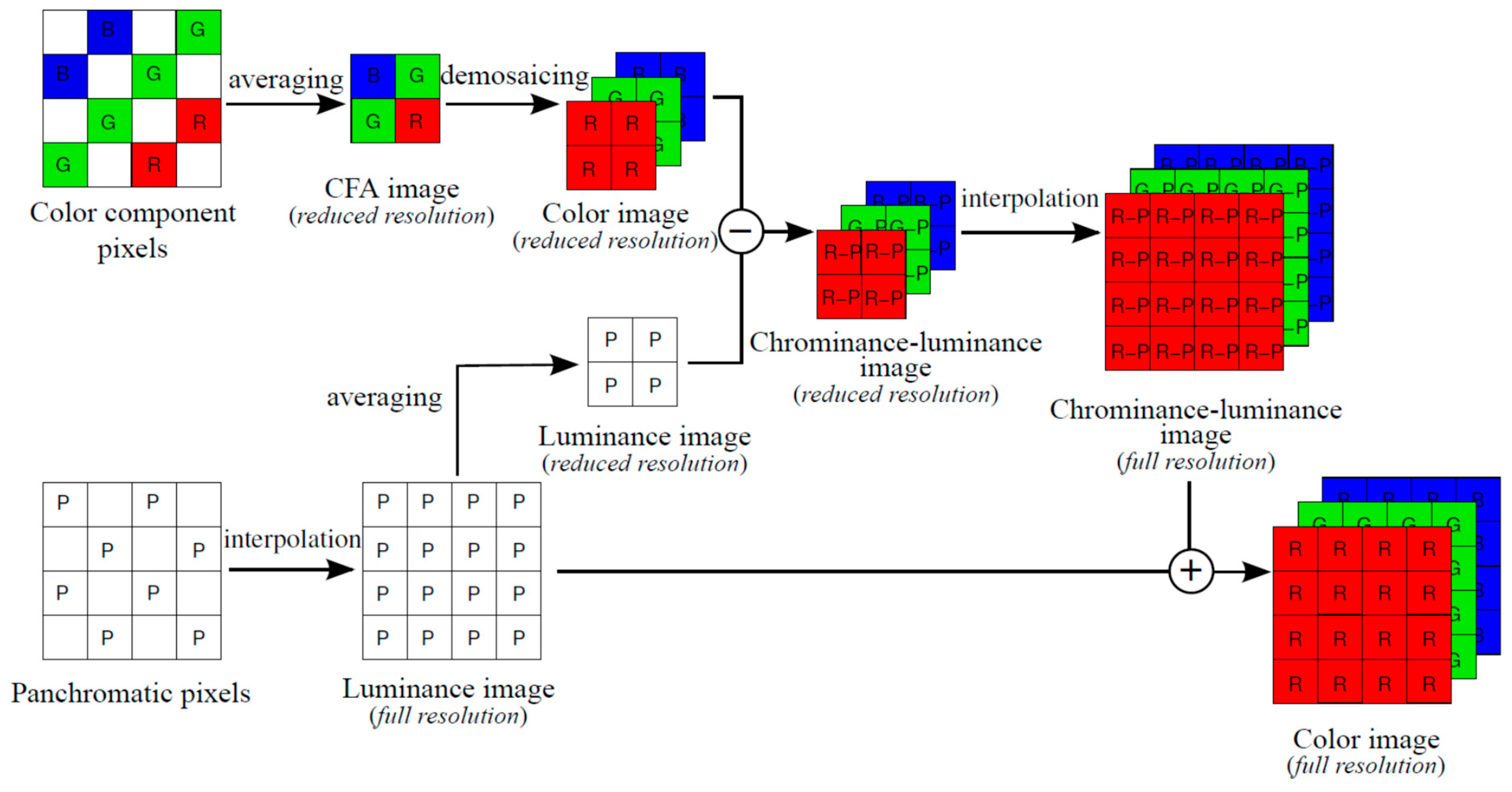
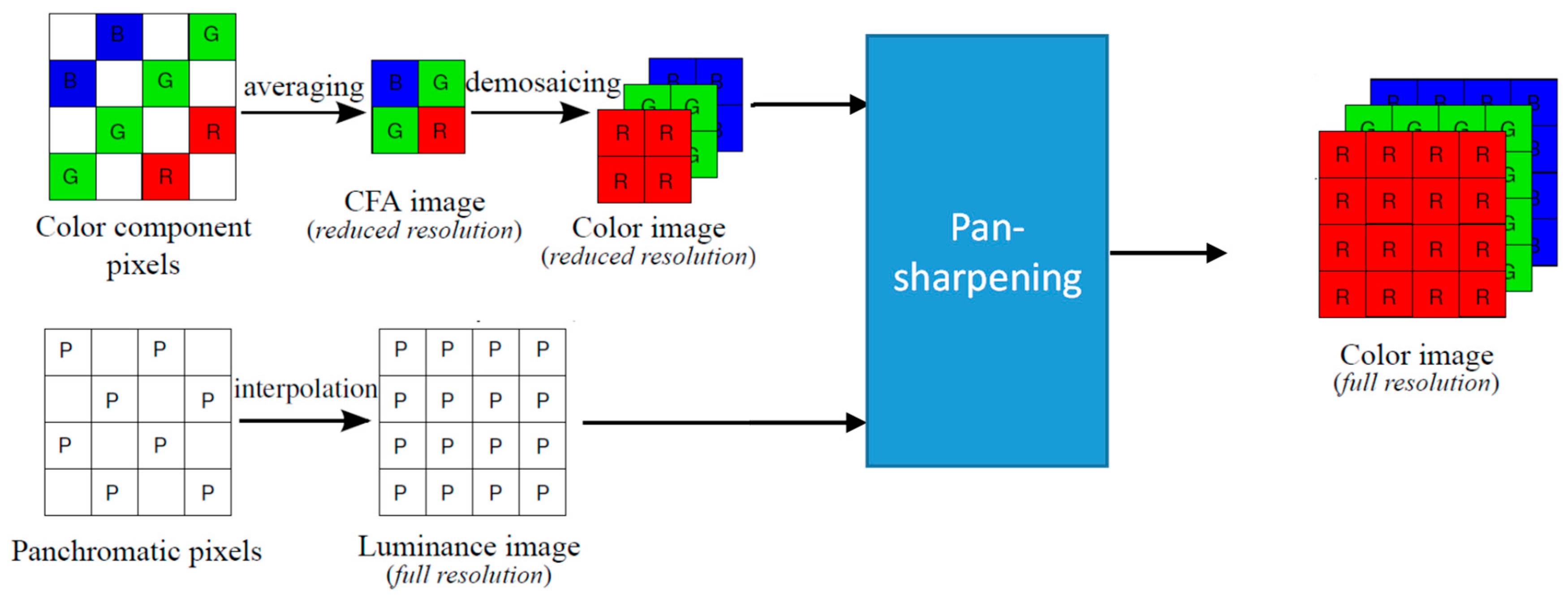

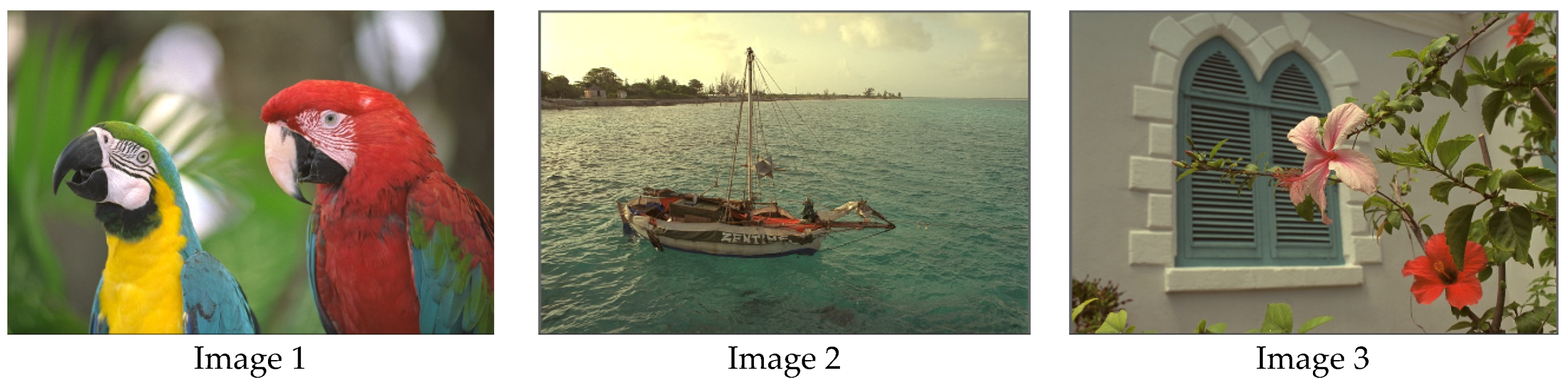
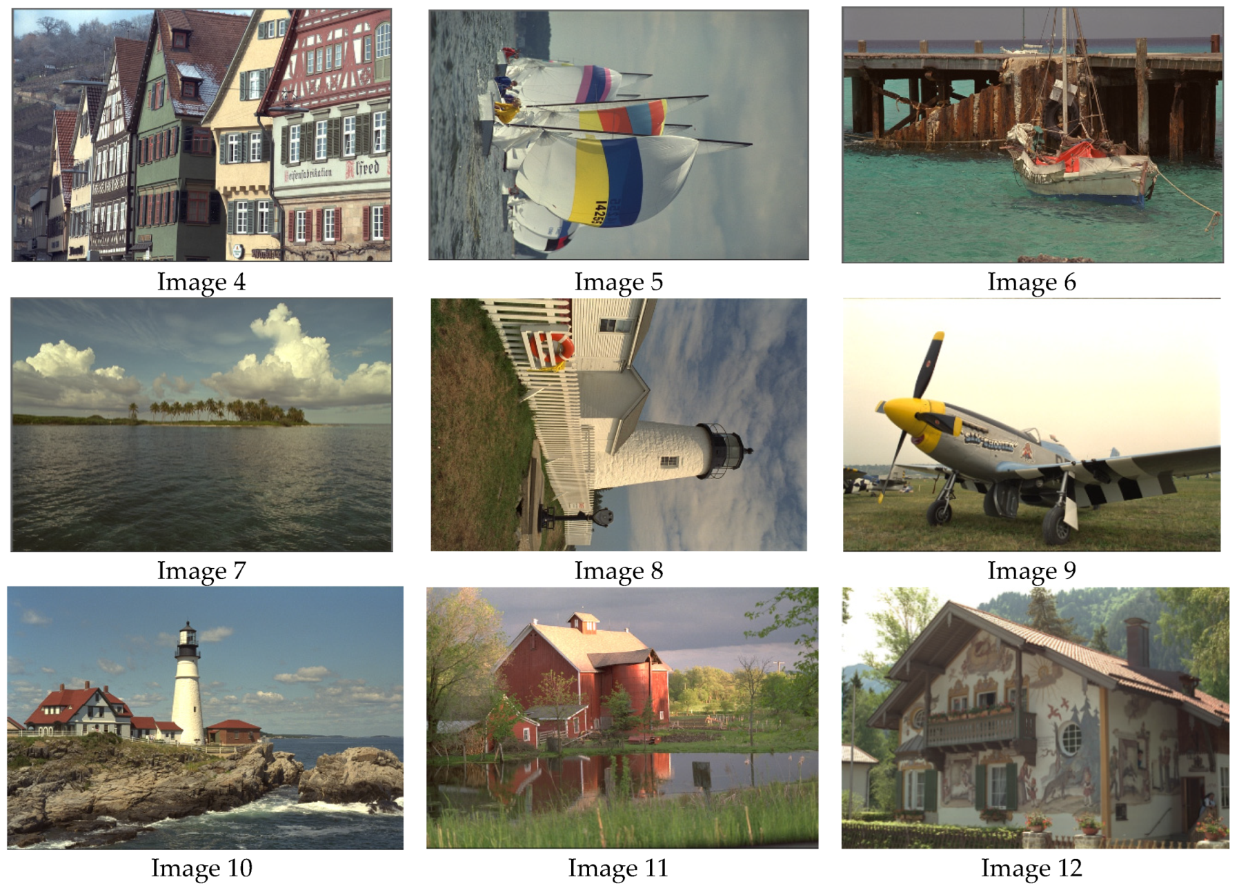
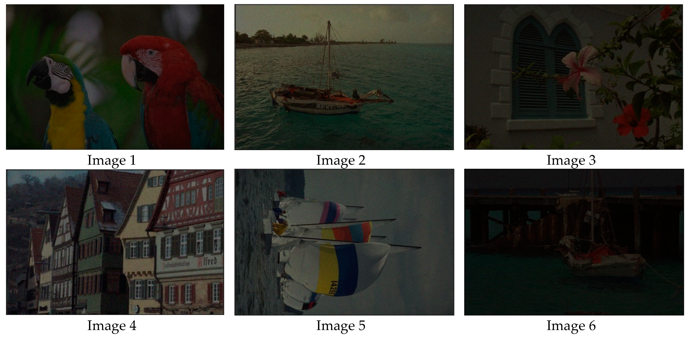

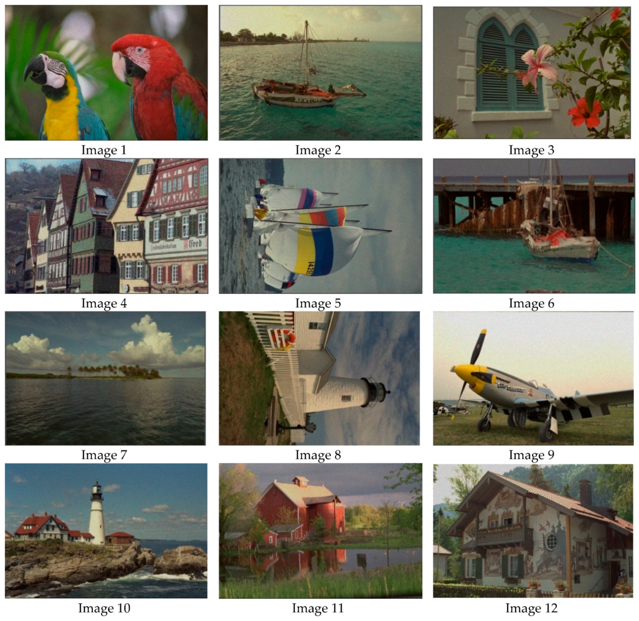
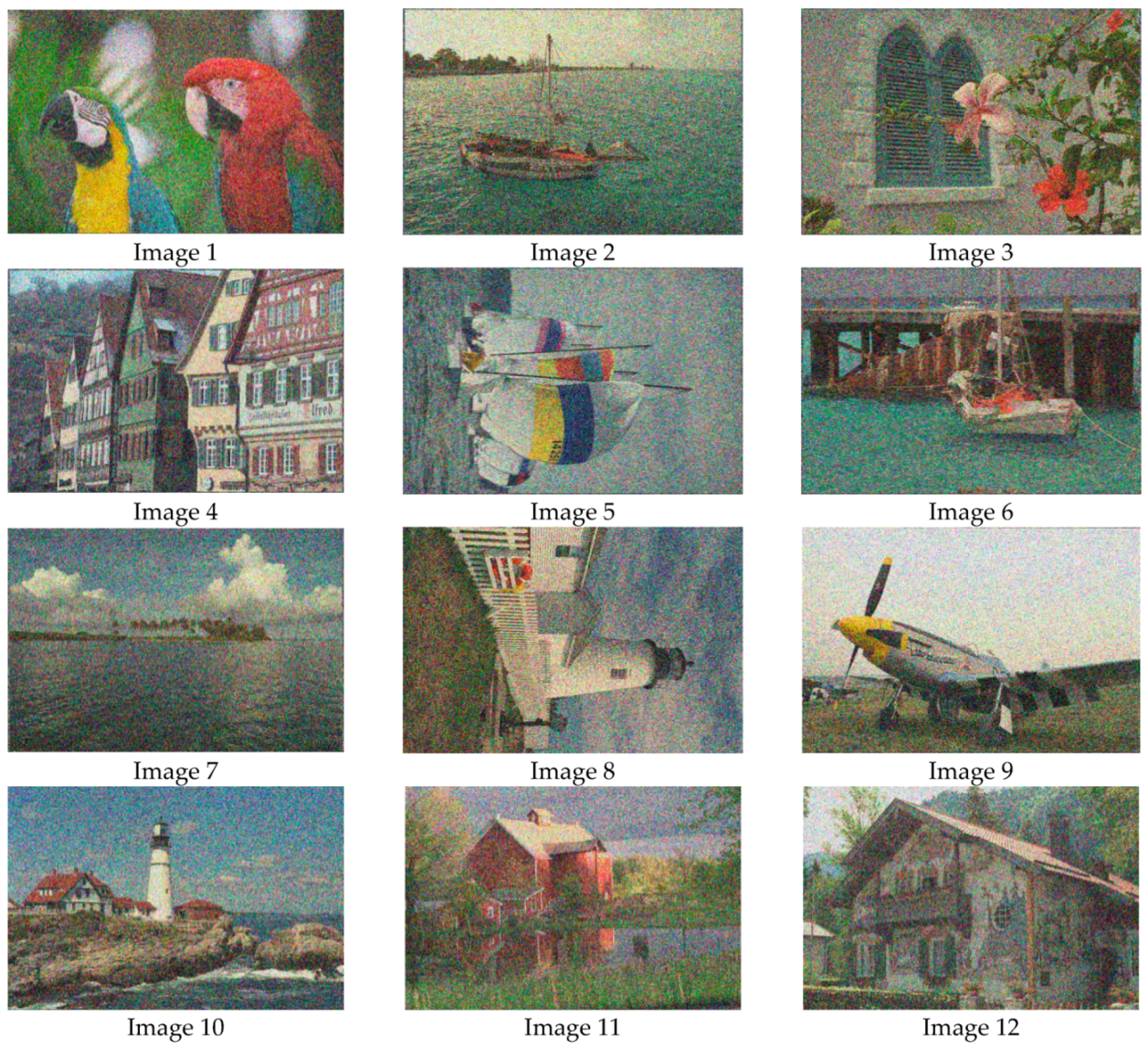
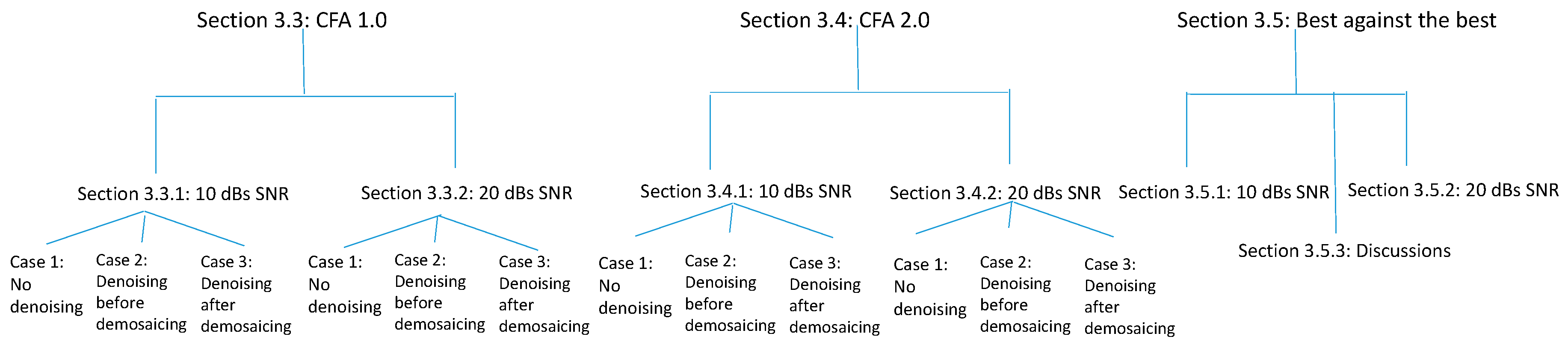

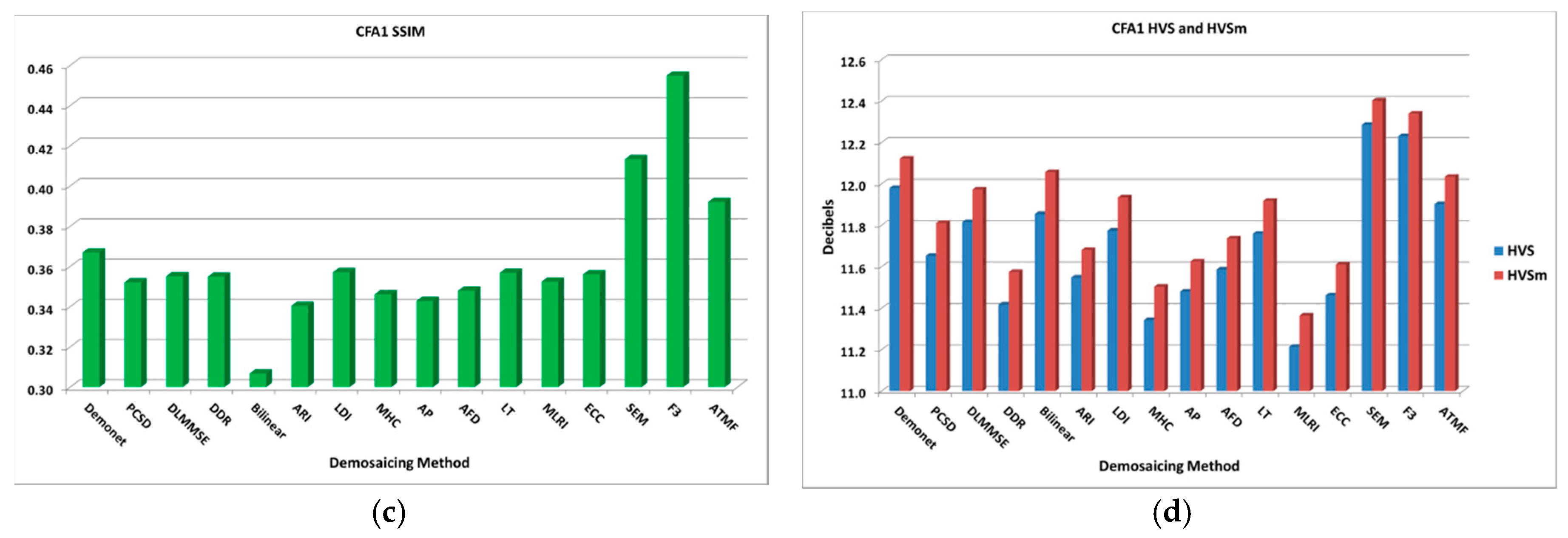


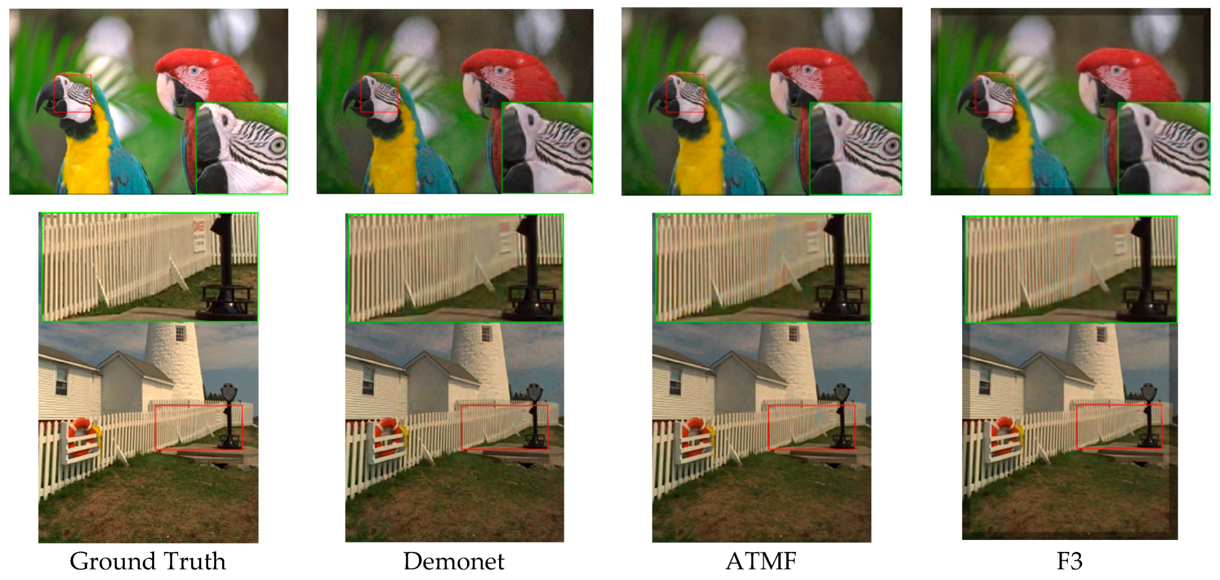
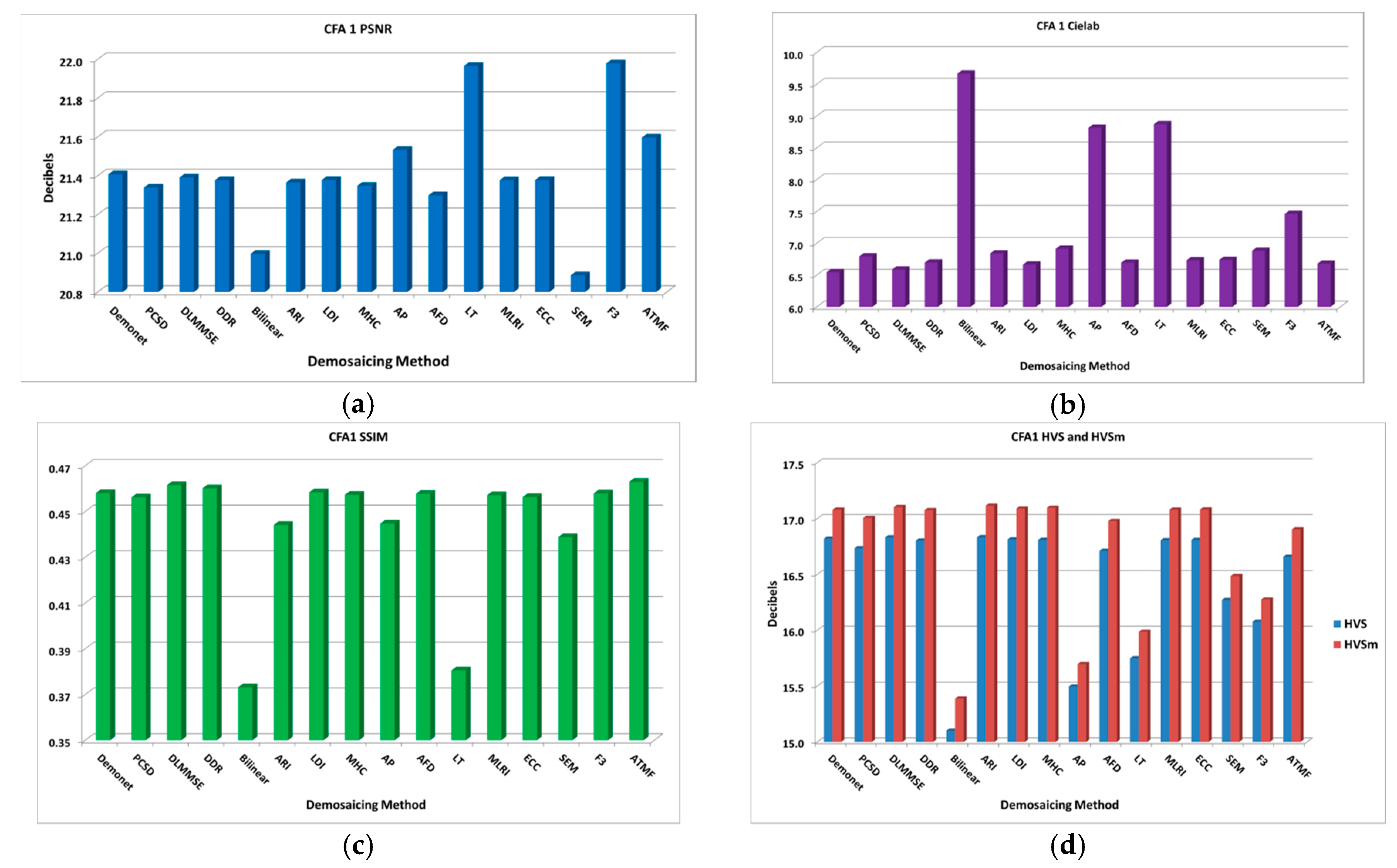
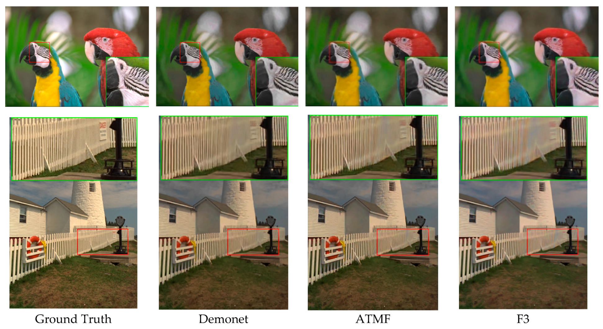
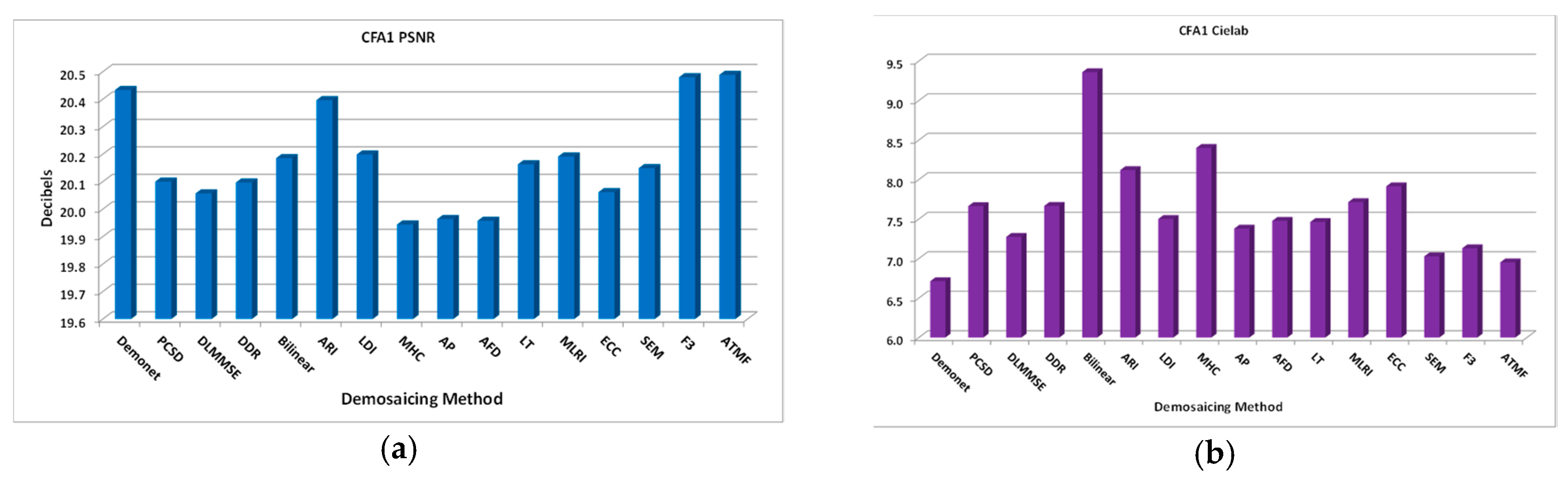
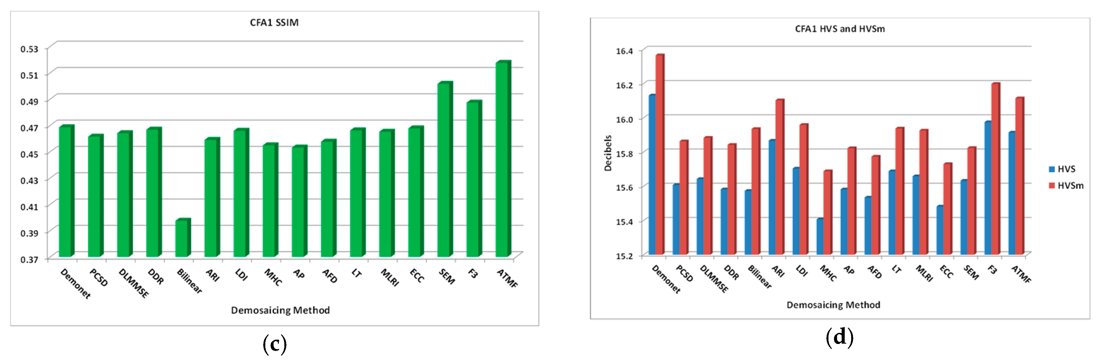

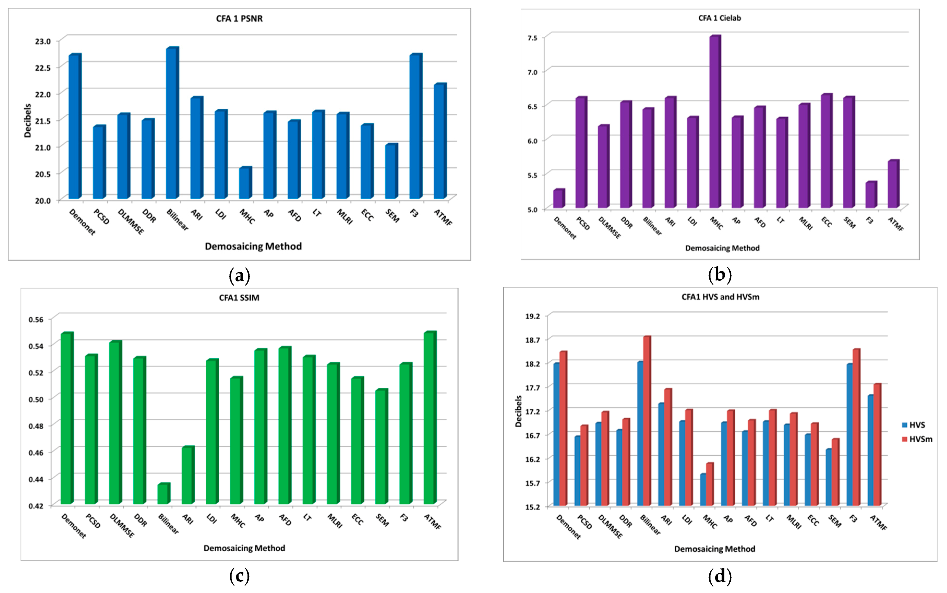
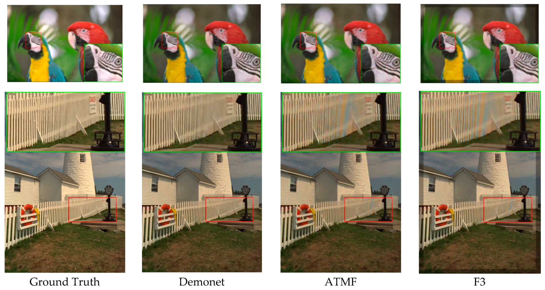
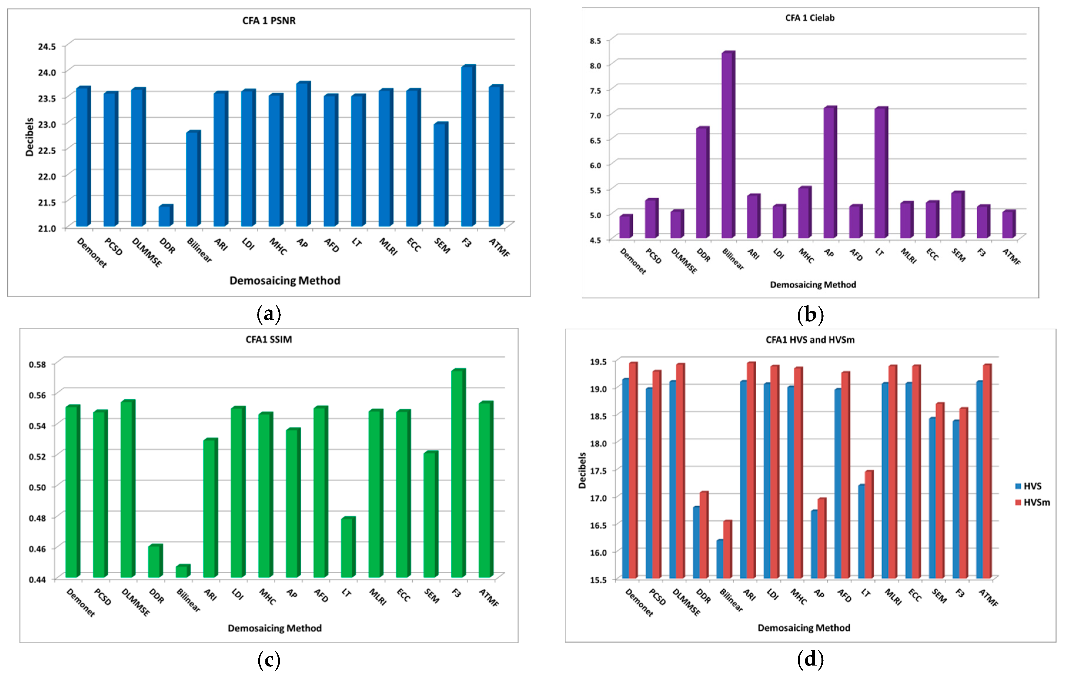
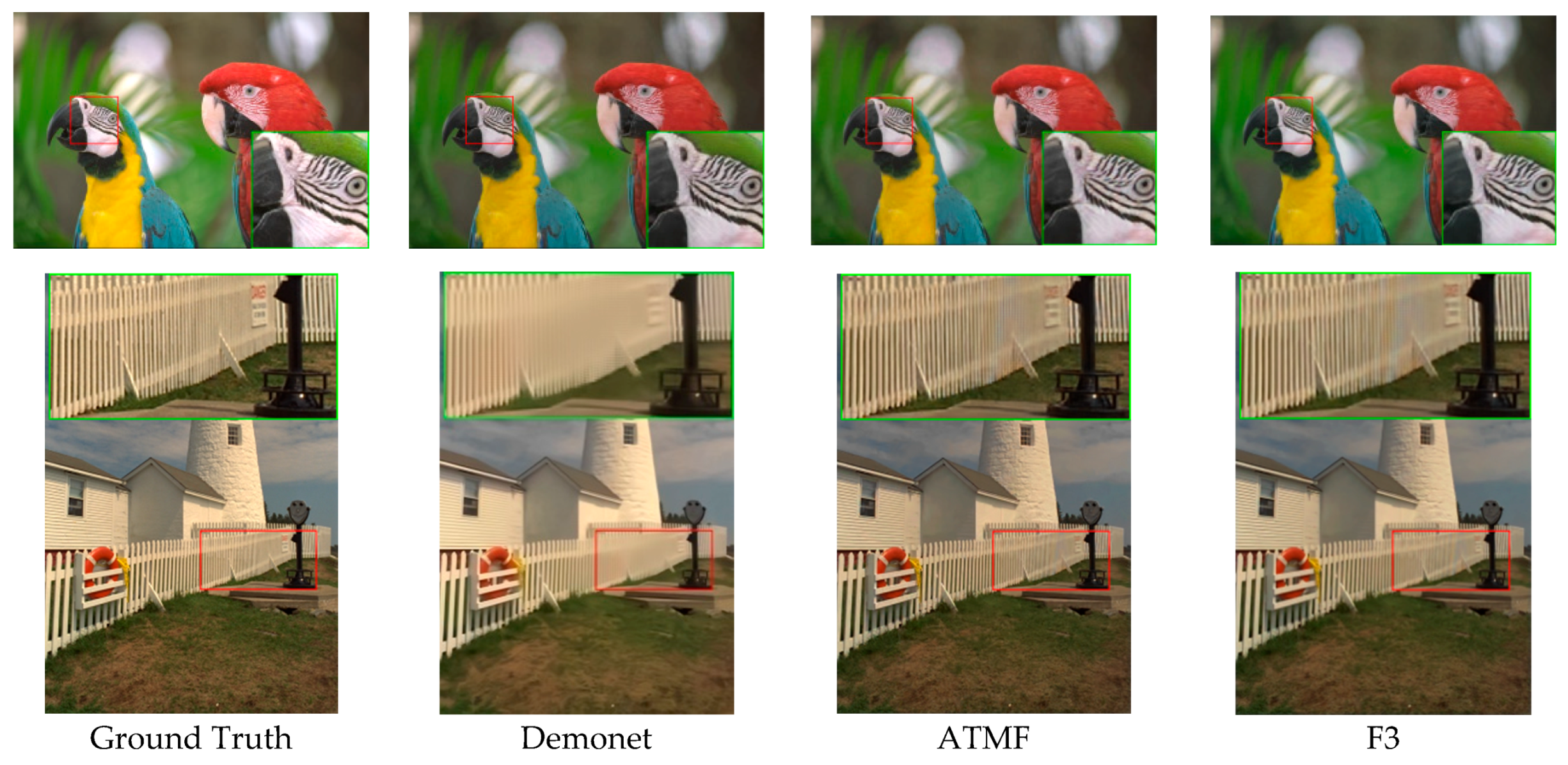


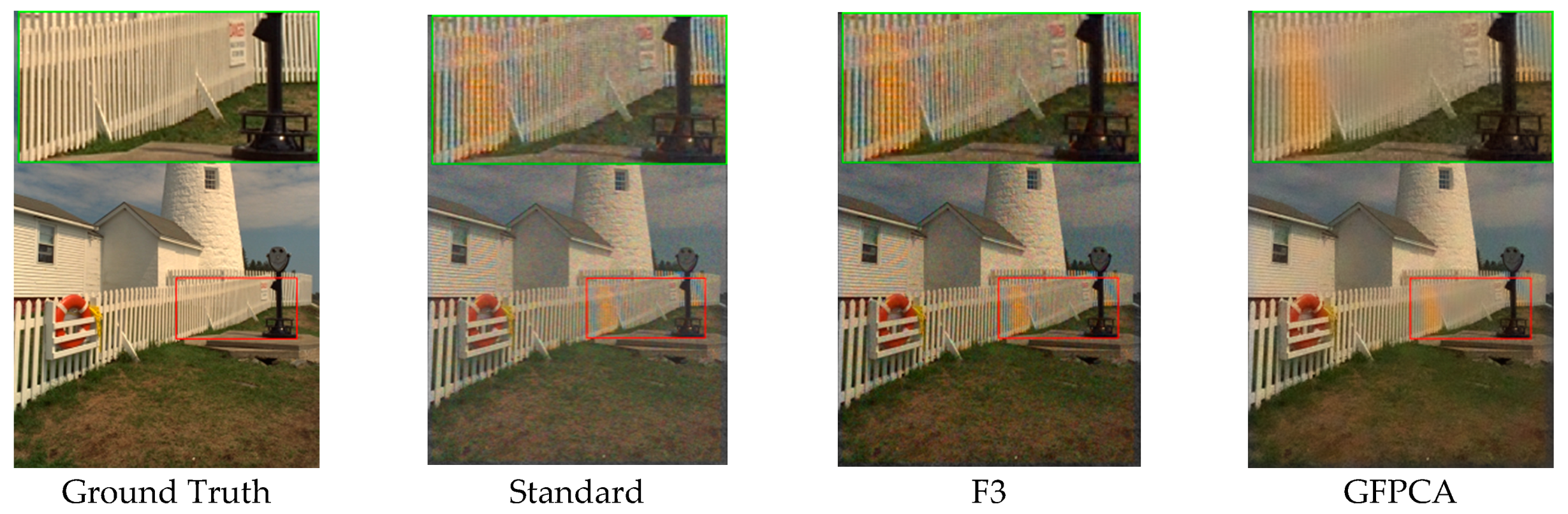

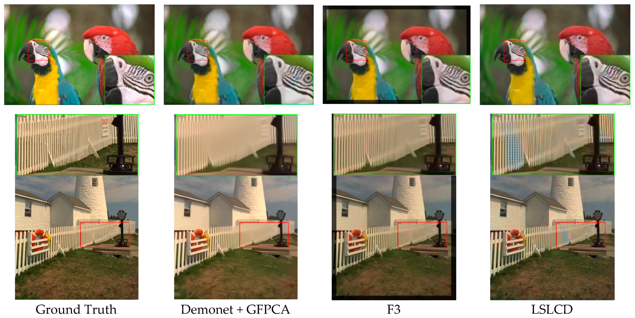
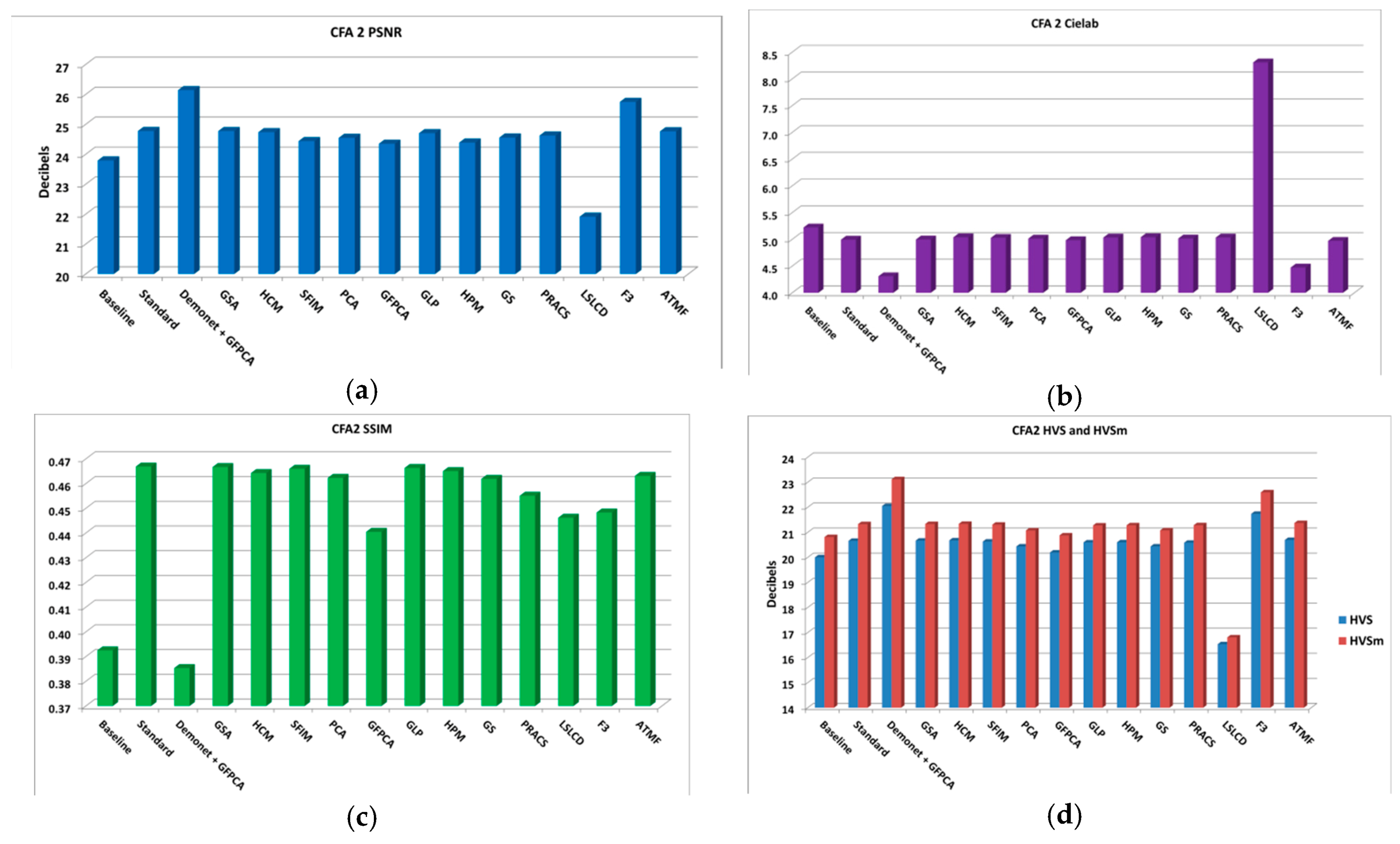
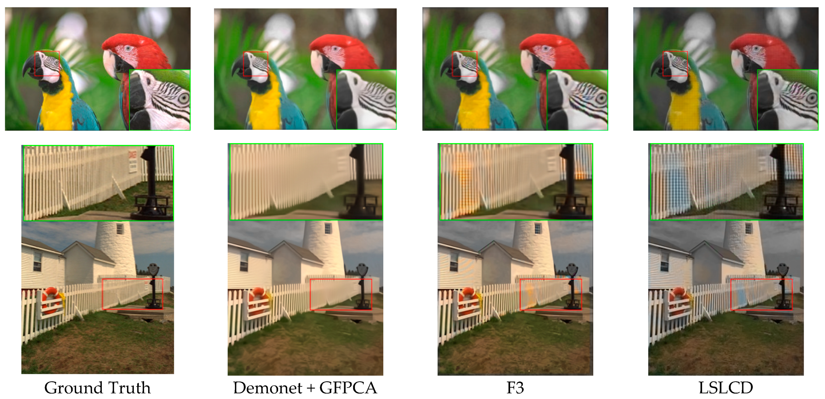
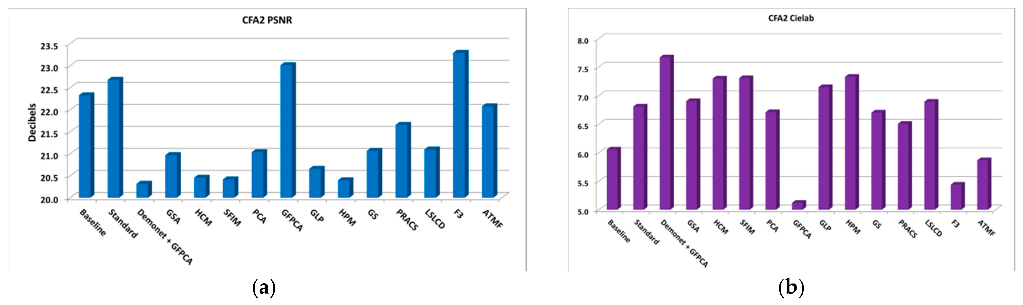
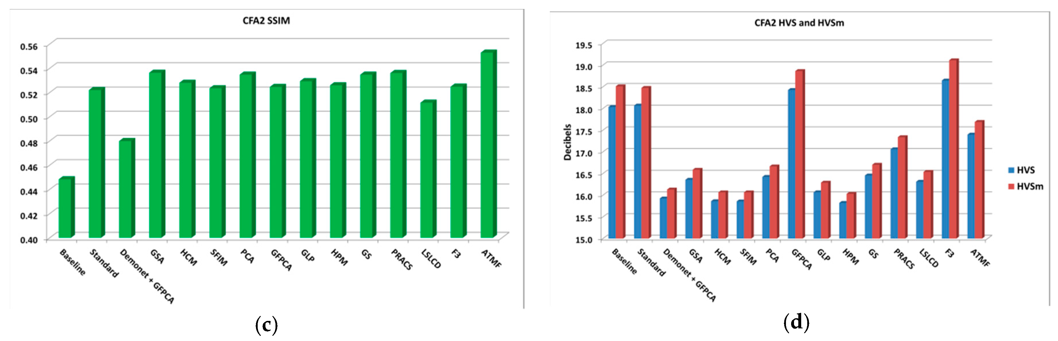
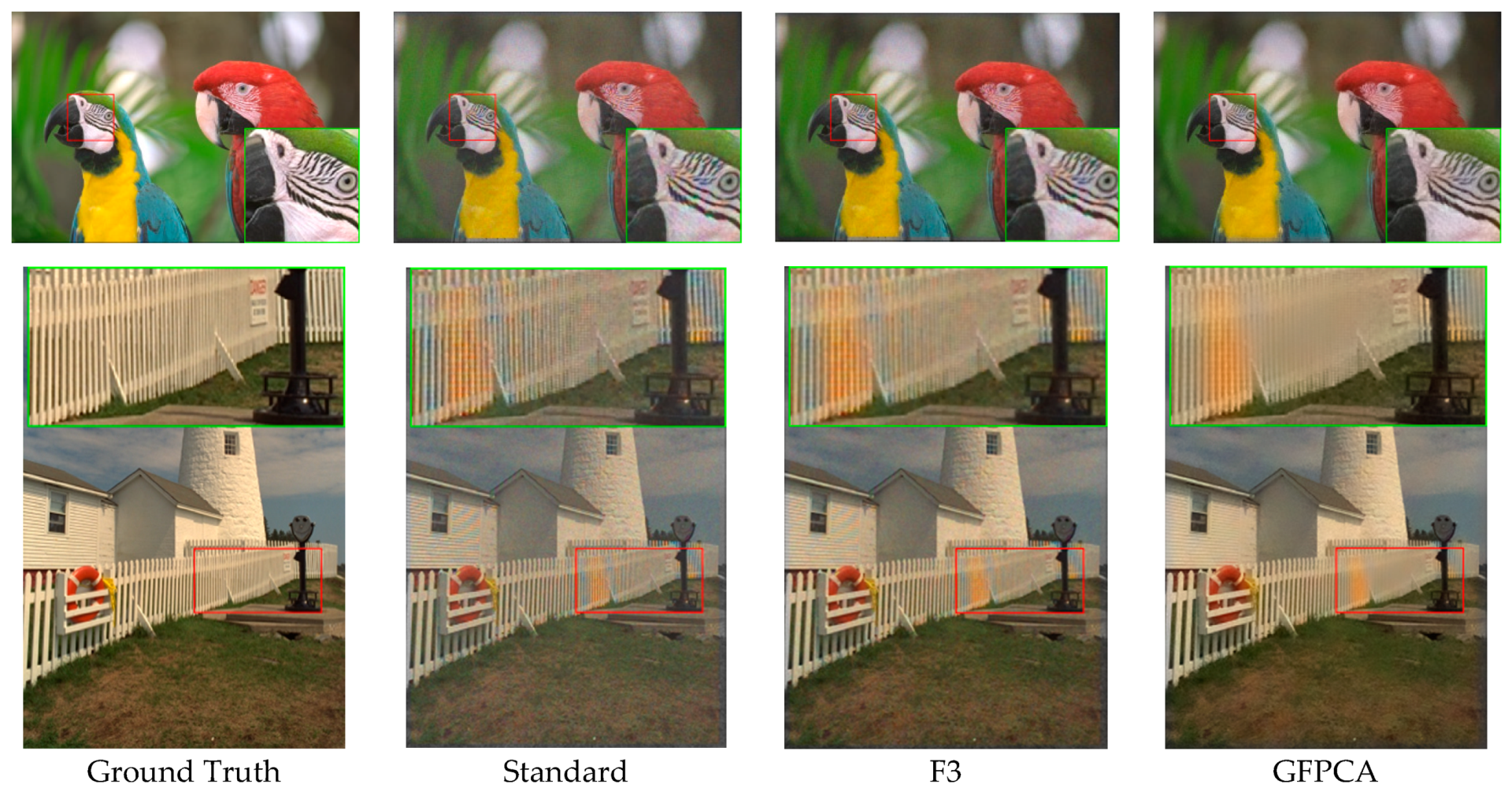
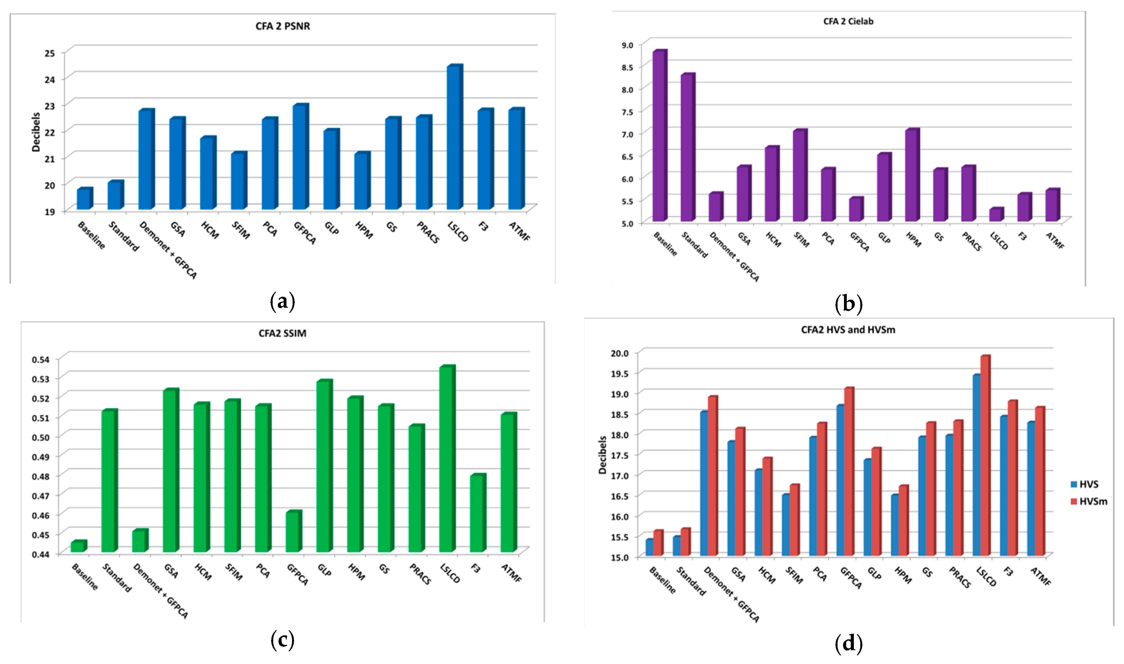
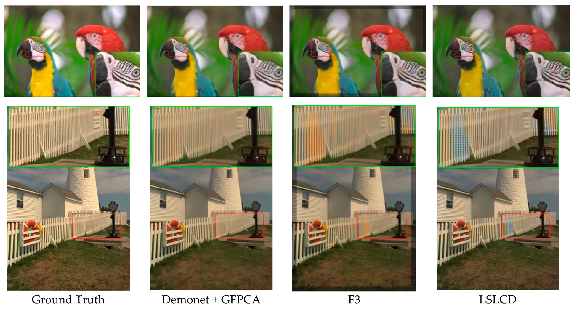
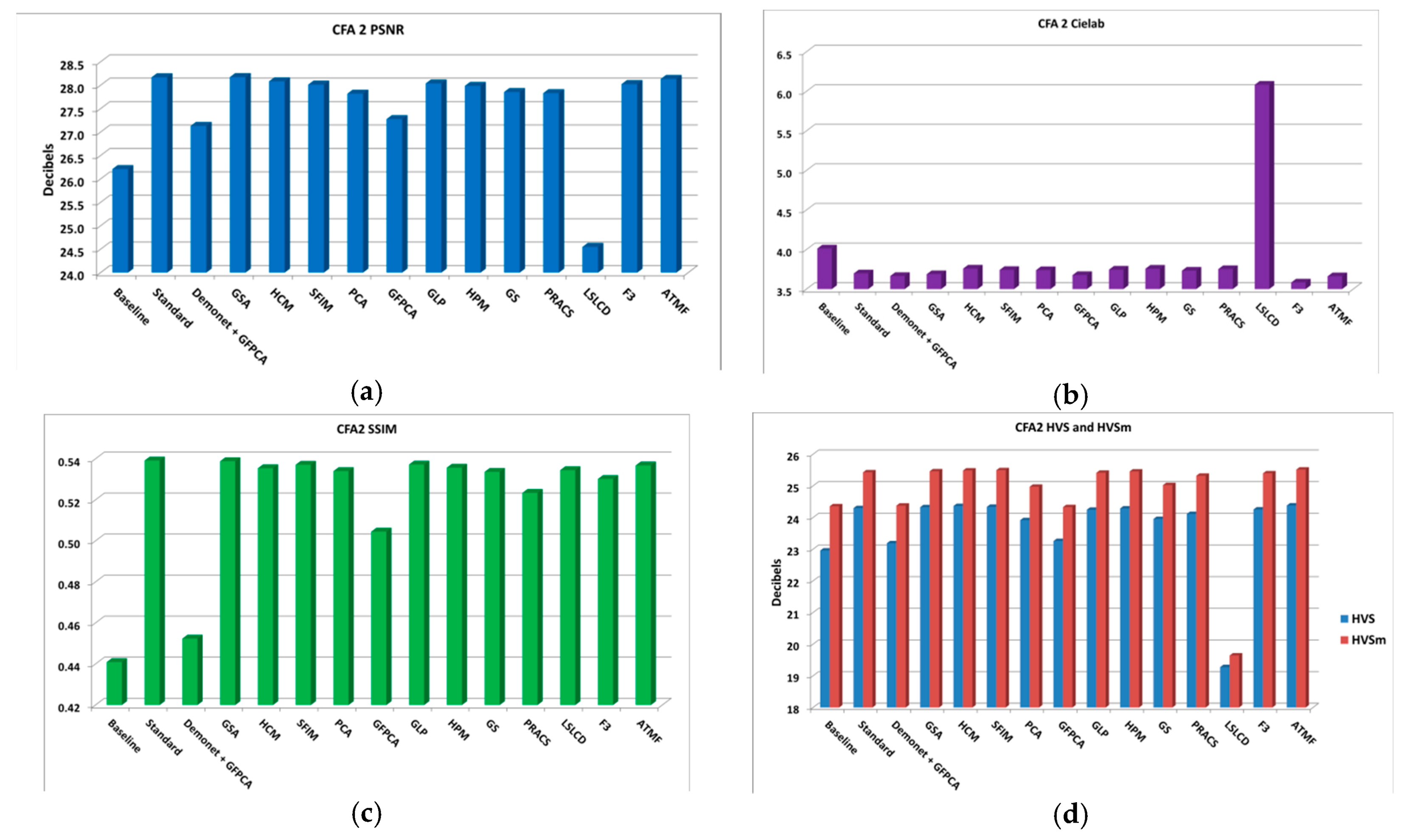
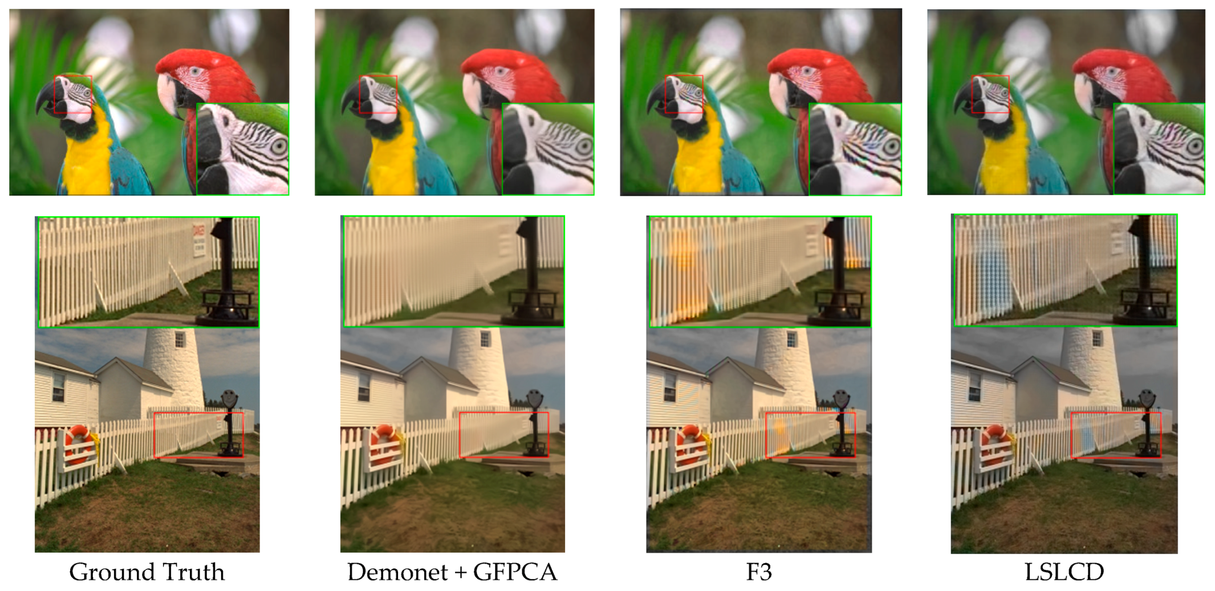
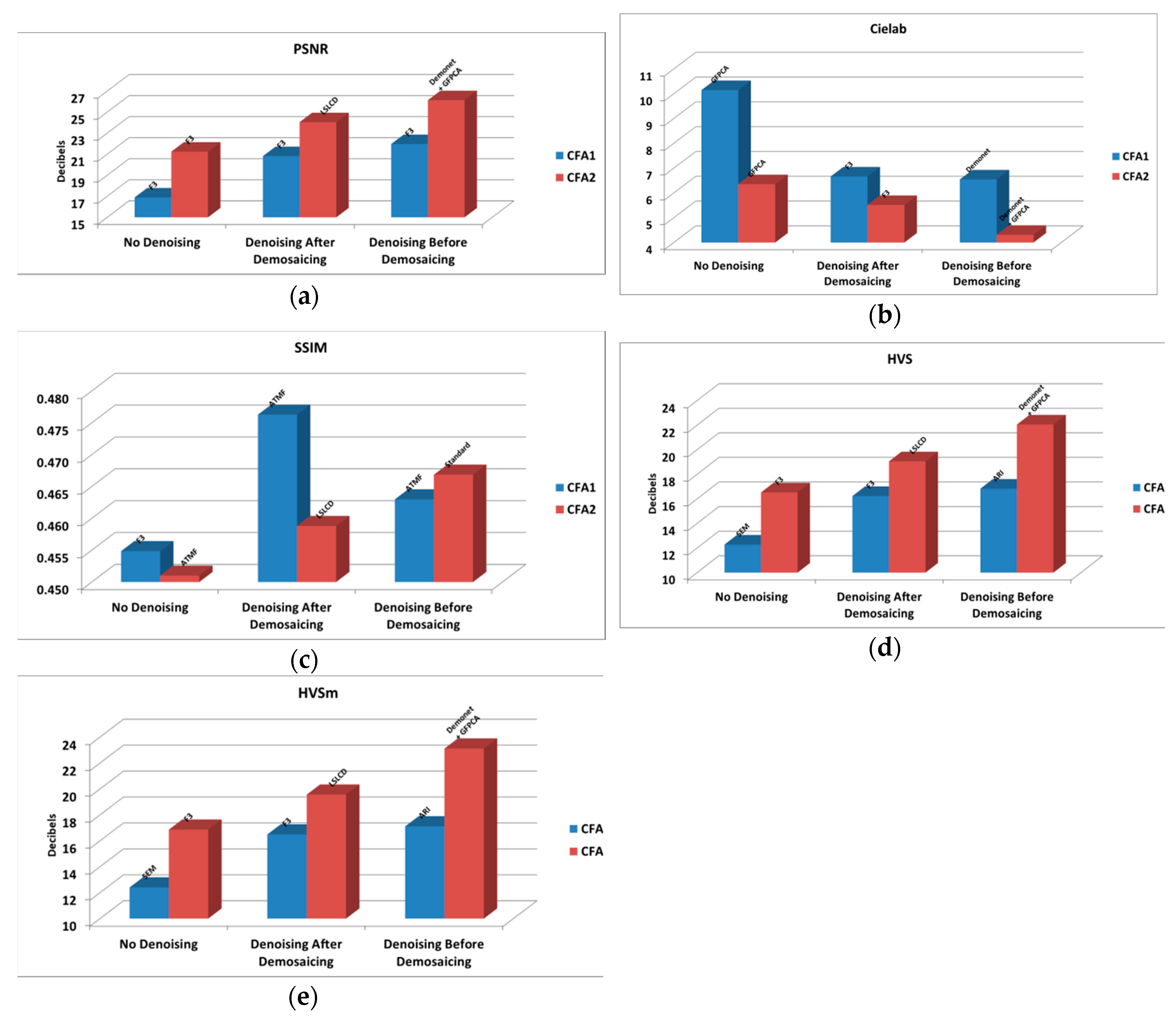
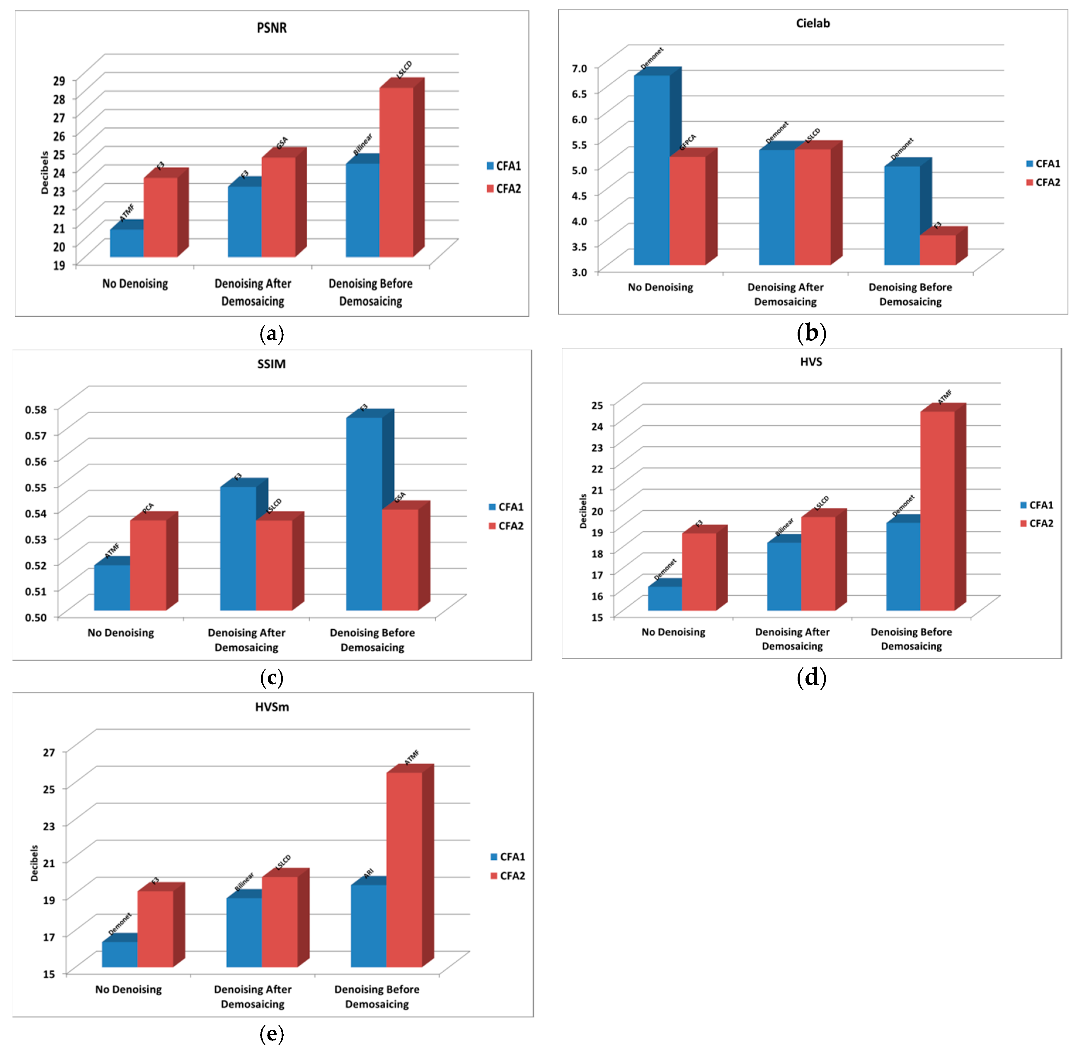
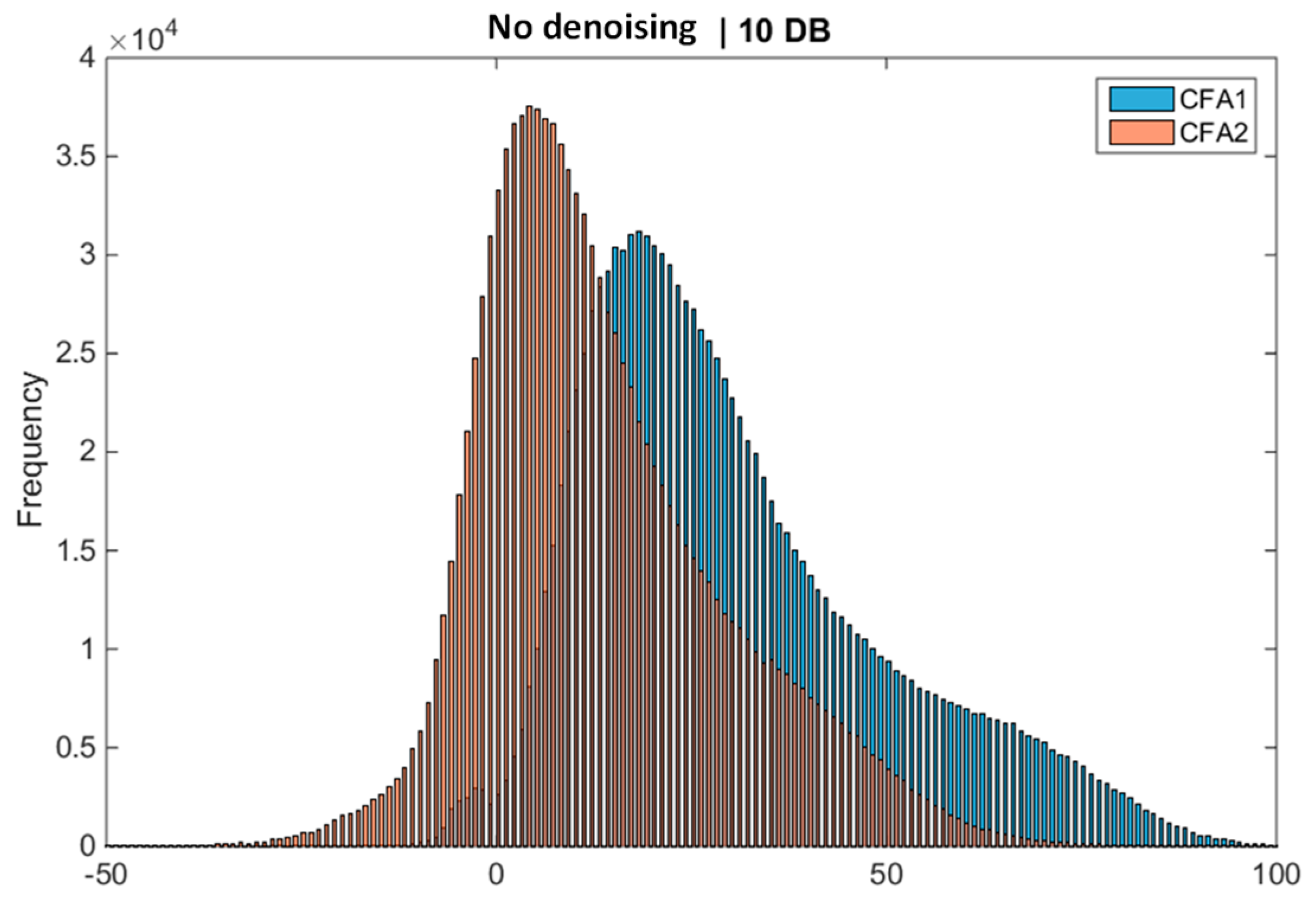

| Measure | Reference | Spearman Correlation | Kendall Correlation |
|---|---|---|---|
| HVS-m | Ponomarenko, N.; et al. [59] | 0.984 | 0.948 |
| HVS | Egiazarian, K.; et al. [58] | 0.895 | 0.712 |
| NQM | Damera-Venkata, N.; et al. [60] | 0.857 | 0.673 |
| DCTune | Watson, A. B.; et al. [61] | 0.829 | 0.712 |
| UQI | Wang, Z.; Bovik, A. C. [62] | 0.550 | 0.438 |
| PSNR | Peak Signal to Noise Ratio [55] | 0.537 | 0.359 |
| SSIM | Structural similarity [56] | 0.406 | 0.358 |
| VIF | Sheikh, H. R.; Bovik, A. C. [63] | 0.377 | 0.255 |
| PQS | Miyahara, M.; Kotani, K.; Algazi, V. R. [64] | 0.302 | 0.242 |
| Metrics | CFA | No Denoising/Best Algorithm | Denoising After Demosaicing/Best Algorithm | Denoising Before Demosaicing/Best Algorithm |
|---|---|---|---|---|
| PSNR (dB) | 1.0 | 16.889/F3 | 20.826/F3 | 21.978/F3 |
| 2.0 | 21.249/F3 | 24.050/LSLCD | 26.141/Demonet+GFPCA | |
| CIELAB | 1.0 | 10.149/GFPCA | 6.664/F3 | 6.545/Demonet |
| 2.0 | 6.354/GFPCA | 5.516/F3 | 4.310/Demonet+GFPCA | |
| SSIM | 1.0 | 0.455/F3 | 0.476/ATMF | 0.463/ATMF |
| 2.0 | 0.451/ATMF | 0.459/LSLCD | 0.467/Standard | |
| HVS (dB) | 1.0 | 12.285/SEM | 16.229/F3 | 16.833/ARI |
| 2.0 | 16.531/F3 | 19.056/LSLCD | 22.053/Demonet+GFPCA | |
| HVSm (dB) | 1.0 | 12.403/SEM | 16.494/F3 | 17.116/ARI |
| 2.0 | 16.868/F3 | 19.568/LSLCD | 23.121/Demonet+GFPCA |
| Metrics | CFA | No Denoising/Best Algorithm | Denoising After Demosaicing/Best Algorithm | Denoising Before Demosaicing/Best Algorithm |
|---|---|---|---|---|
| PSNR (dB) | 1.0 | 20.488/ATMF | 22.821/F3 | 24.059/Bilinear |
| 2.0 | 23.290/F3 | 24.391/GSA | 28.172/LSLCD | |
| CIELAB | 1.0 | 6.713/Demonet | 5.256/Demonet | 4.935/Demonet |
| 2.0 | 5.121/GFPCA | 5.268/LSLCD | 3.584/F3 | |
| SSIM | 1.0 | 0.500/SEM | 0.548/F3 | 0.574/F3 |
| 2.0 | 0.545/Demonet+GFPCA | 0.535/LSLCD | 0.539/GSA | |
| HVS (dB) | 1.0 | 16.130/Demonet | 18.204/Bilinear | 19.142/Demonet |
| 2.0 | 18.646/F3 | 19.415/LSLCD | 24.382/ATMF | |
| HVSm (dB) | 1.0 | 16.365/Demonet | 18.734/Bilinear | 19.444/ARI |
| 2.0 | 19.112/F3 | 19.881/LSLCD | 25.516/ATMF |
© 2019 by the authors. Licensee MDPI, Basel, Switzerland. This article is an open access article distributed under the terms and conditions of the Creative Commons Attribution (CC BY) license (http://creativecommons.org/licenses/by/4.0/).
Share and Cite
Kwan, C.; Larkin, J. Demosaicing of Bayer and CFA 2.0 Patterns for Low Lighting Images. Electronics 2019, 8, 1444. https://doi.org/10.3390/electronics8121444
Kwan C, Larkin J. Demosaicing of Bayer and CFA 2.0 Patterns for Low Lighting Images. Electronics. 2019; 8(12):1444. https://doi.org/10.3390/electronics8121444
Chicago/Turabian StyleKwan, Chiman, and Jude Larkin. 2019. "Demosaicing of Bayer and CFA 2.0 Patterns for Low Lighting Images" Electronics 8, no. 12: 1444. https://doi.org/10.3390/electronics8121444
APA StyleKwan, C., & Larkin, J. (2019). Demosaicing of Bayer and CFA 2.0 Patterns for Low Lighting Images. Electronics, 8(12), 1444. https://doi.org/10.3390/electronics8121444