Article

Wideband Performance Comparison between the 40 GHz and 60 GHz Frequency Bands for Indoor Radio Channels

1
Signal Theory and Communications Department, University of Vigo, 36310 Vigo, Spain
2
Department of Information Technology, Ghent University/imec, 9000 Gent, Belgium
*
Author to whom correspondence should be addressed.
Electronics 2019, 8(11), 1234; https://doi.org/10.3390/electronics8111234
Submission received: 27 September 2019 / Revised: 22 October 2019 / Accepted: 26 October 2019 / Published: 29 October 2019
(This article belongs to the Special Issue Millimeter-Wave (mmWave) Communications)

Abstract

:
When 5G networks are to be deployed, the usability of millimeter-wave frequency allocations seems to be left out of the debate. However, there is an open question regarding the advantages and disadvantages of the main candidates for this allocation: The use of the licensed spectrum near 40 GHz or the unlicensed band at 60 GHz. Both bands may be adequate for high performance radio communication systems, and this paper provides insight into such alternatives. A large measurement campaign supplied enough data to analyze and to evaluate the network performance for both frequency bands in different types of indoor environments: Both large rooms and narrow corridors, and both line of sight and obstructed line of sight conditions. As a result of such a campaign and after a deep analysis in terms of wideband parameters, the radio channel usability is analyzed with numerical data regarding its performance.

1. Introduction

A society without wireless communication is unthinkable nowadays. In the latest decades, people and enterprises have used wireless communication every day and the evolution in wireless technologies has redefined how people work and communicate. Beside consumers, enterprises have also embraced this revolution to work faster and more efficiently.
In 1982, the first generation of mobile communications (1G) was released: Analog-based and very limited, as voice service was its only capability. Ten years later, the digital version appeared (2G), offering the possibility of sending data through the network in the form of what was called short message system (SMS). The following generation, 3G, along with the then recently introduced smartphones, offered the possibility of sharing multimedia data, faster web browsing and even video calling. The fourth generation, 4G, increased the performance of the previous generation in terms of data rate. The next revolution in wireless communication is right around the corner: The fifth generation (5G). This technology promises higher speeds and lower latencies. To accommodate this new generation, frequency bands both below and over current 4G ones will be used [1]. Nowadays, with the emergence of streaming platforms allowing via a mobile connection to watch movies and series or even to play games, the consumer is demanding even more data rate in order to be able to keep up with the increasing quality of the content. 5G will try to provide a solution to all these demands and even more, like the low latency required in vehicle to vehicle or vehicle to infrastructure communications for autonomous cars.
When designing 5G, some doubts arose on the usage of millimeter wave frequency bands. Rappaport et al. supported that 5G would get consistent coverage at 38 GHz by installing base stations with a 200-meter cell-radius in dense urban environments [2]. Once any worry related to the usability of such frequencies was removed, a normalization process was started by consortia (like 3GPP) and institutions (like ITU). Today some public administrations (like FCC) have announced auctions of spectrum parts at millimeter wave frequencies for 5G [3]. Alternatively, there is an unlicensed band around 60 GHz that is also well positioned to succeed as a candidate for providing high performance services based on radio communication systems [4]. Both frequency bands allow high rate traffic and the final decision depends on a deep analysis of their advantages and disadvantages.
Facing the 5G expectation, a precise channel characterization is necessary, as network planners are concerned on achieving the required quality of service. However, indoor scenarios still need deeper analysis to assure that propagation within such environments fits within the expected performance of those frequency bands. Thus, this paper proposes an experimental analysis from the results of a measurement campaign at two frequency channels in the millimeter wave range: 40 GHz and 60 GHz. The measurements are performed in a corridor in both a line of sight (LOS) and obstructed line of sight (OLOS) scenarios, and in an ordinary auditorium used for teaching activities.
As a result, this paper provides wideband propagation parameters at both frequency bands and in different environments, giving an insight into their characteristics and also helping network planners in selecting the most adequate frequency channels. We detected that the effect of multipath would be less important in the 60 GHz band, as attenuations by propagation mechanisms will reduce the influence of contributions with larger delays. In general, the root mean square (RMS) delay spread is larger at 40 GHz than at 60 GHz, which could limit the usability for wideband systems. The worst case also occurs in OLOS conditions, which cannot be neglected in a real world indoor radio link.
After this introduction, the setup of the measurements is discussed in Section 2, devoted to materials and methods. This section also contains the description of the environments, the post processing techniques and the ray-tracing analysis used to check the origin of the observed effects. Section 3 contains the wideband results at both the corridor and the auditorium environments. This section relates the power delay profile (PDP) to the shape of the environment, with the help of the ray-tracing analysis, and it also shows the main wideband parameters as time spread and coherence bandwidth. The discussion of these results is handled in Section 4. Finally, Section 5 summarizes the conclusions.

2. Materials and Methods

This section describes the measurement, analysis and interpretation of the collected data: It starts with the measurement setup and procedure, it continues with the measurement environments and the post processing applied to the raw data. It finishes with the ray-tracing analysis used to explain the different observed effects within the indoor environments.

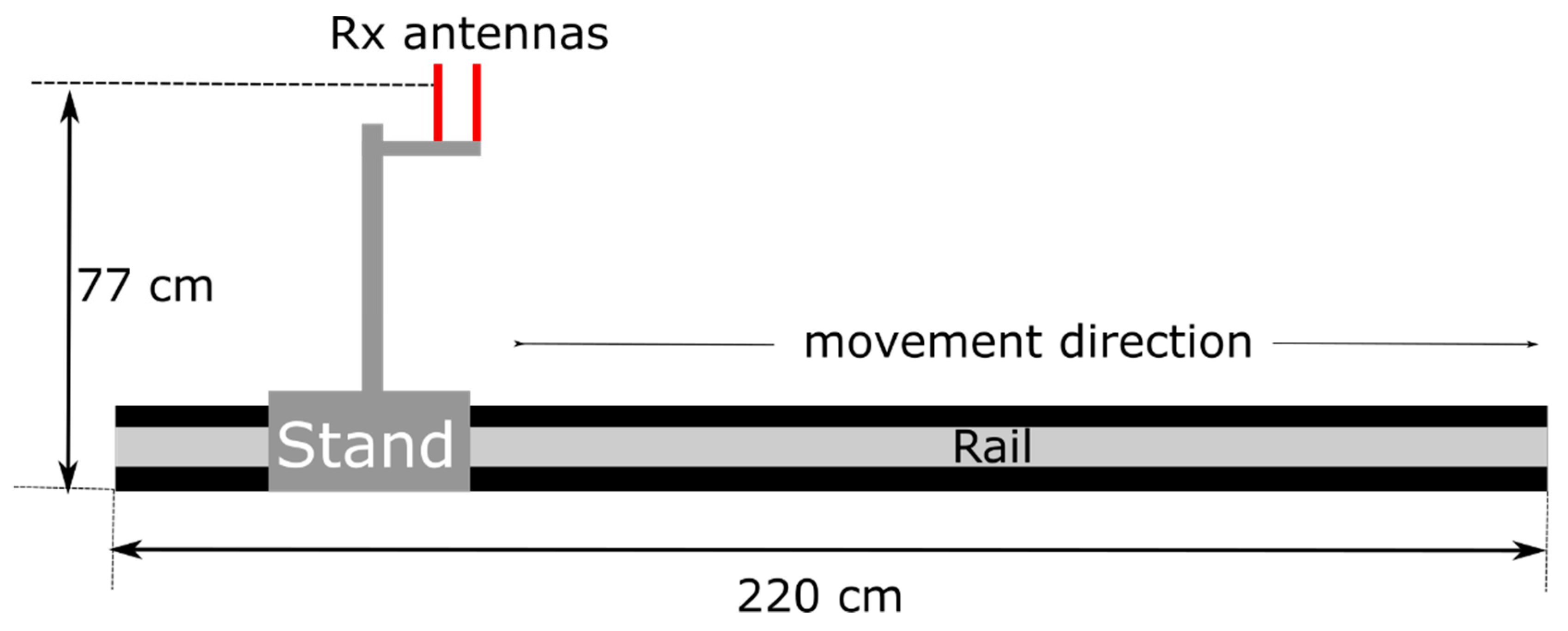
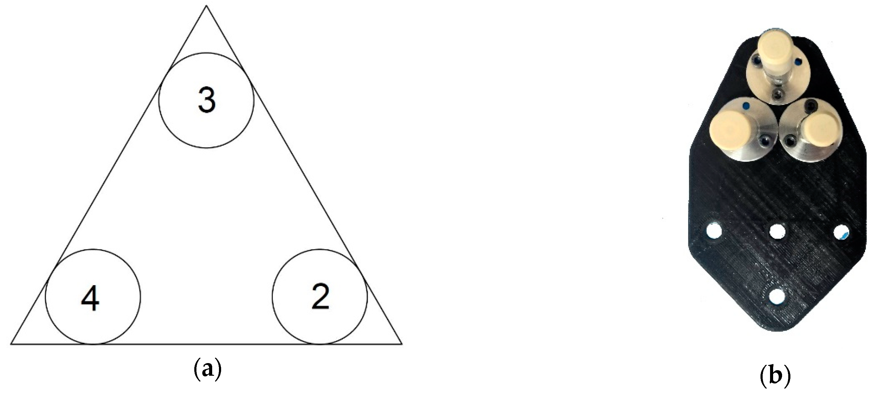
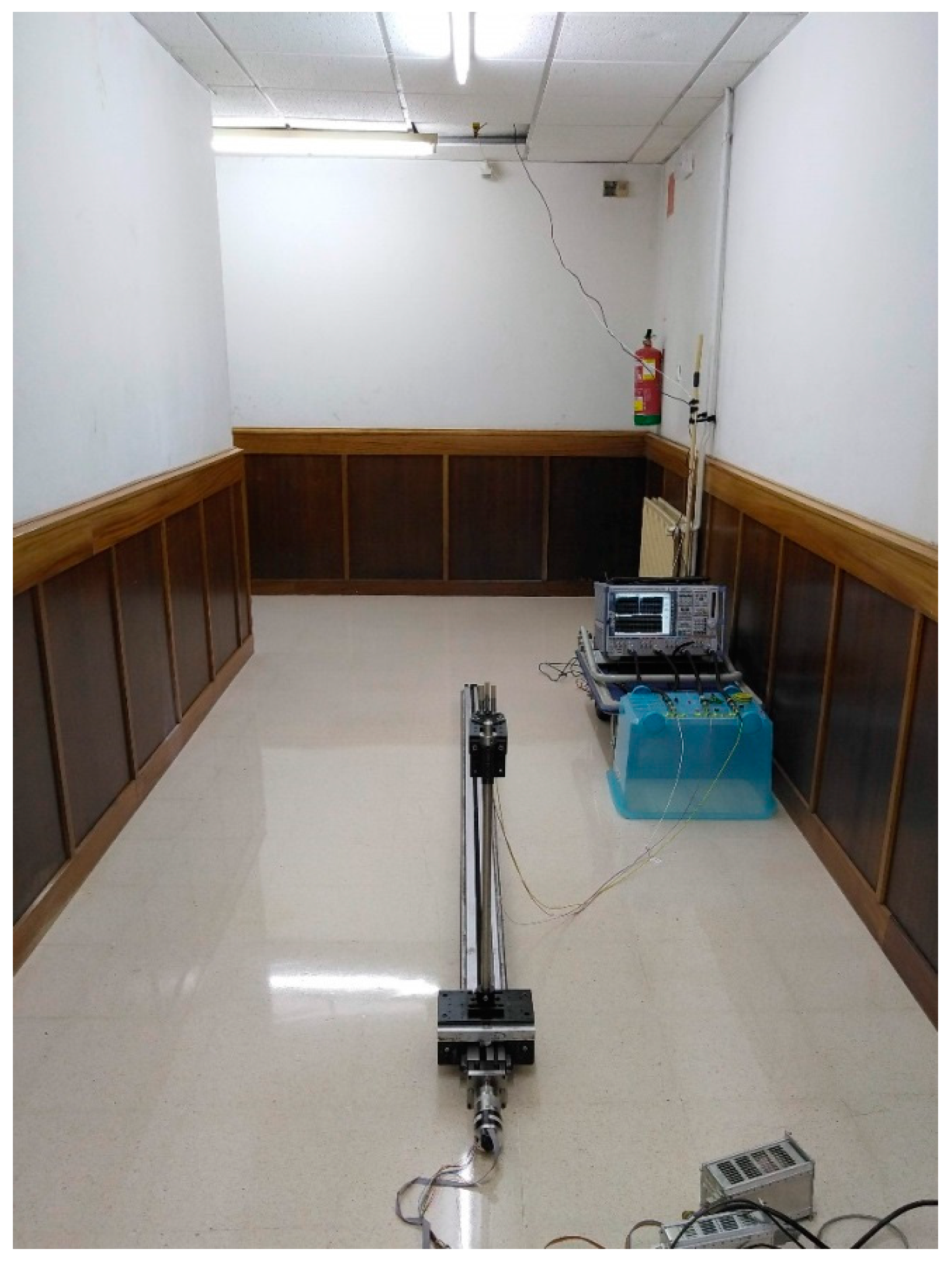
2.1. Measurement Setup and Procedure

Measurements followed the frequency swept method [5]. A Rhode & Schwarz ZVA67 vector network analyzer (VNA) (Rohde & Schwarz, Munich, Germany) executed the measurements of the frequency response of the radio channel. This equipment transmits a frequency-swept signal in the band of interest and gathers the corresponding received signal at the other ends. It also computes the S-parameters of the measured channel as a function of the frequency. To measure at 40 GHz, the transmitter was connected to an amplifier through a 4 m coaxial cable and then to the antenna through a 1 m coaxial cable, making this way a total length of 5 m. At 60 GHz only the 4 m cable was necessary, as the amplifier was a wave guide one and was connected directly to the transmitting antenna. Furthermore, the receiver end consisted of three omnidirectional antennas connected to three VNA receiving ports through three 2 m coaxial cables. Despite future mobile terminals working at millimeter wave frequencies will probably use directive antennas that will filter some multipath components; by using omnidirectional ones in our measurement system we will be able to get a better idea about all the multipath components present in the environments.
The measured frequency bands extend 3 GHz around 41.5 GHz and 60.5 GHz. Each complex frequency response comprises 1001 equally separated frequency samples resulting in a frequency resolution of 3 MHz. A thru calibration of the measurement setup was performed before the field measurements were taken.
The transmitting antenna is attached to the ceiling, whereas the three receiving antennas are mounted close to each other on a stand placed over a straight-line automatized rail, as depicted in Figure 1. Those antennas are mounted in an equilateral triangle with sides of 4 cm for the 40 GHz case and 2.5 cm for the 60 GHz one, following the scheme of Figure 2. These distances are equivalent to 5.3 wavelengths at 40 GHz and 5 wavelengths at 60.5 GHz. The measured mutual coupling shows values below −35 dB and −25 dB at 40 GHz and 60.5 GHz, respectively. The antennas were placed 77 cm above the floor. The antenna labeled as “3” was the closest to the transmitter; the other two are labeled as “2” and “4”. Note that the number of the antenna corresponds with the S parameter measured on the VNA, considering label “1” of the transmitter antenna. For example, S31 corresponds to the channel response of receiver antenna number “3”.
The receiver antennas move over a certain distance on the rail, controlled by an indexer and a laptop. The movement of the stand occurs along 220 cm, in steps of 1.875 mm for the 40 GHz channel and 1.25 mm for the 60 GHz channel. These step lengths are a quarter of the wavelength of their corresponding center frequency. Measurements are repeated with the rail placed at different positions along the corridor, enlarging the entire measurements longer than the length of the rail itself.
A tailor-made Matlab program was developed to capture and process the data. This program runs on a laptop connected to the indexer controlling via a serial RS232 connection the step-by-step motor of the rail and to the VNA using TCP/IP over a UTP cable.

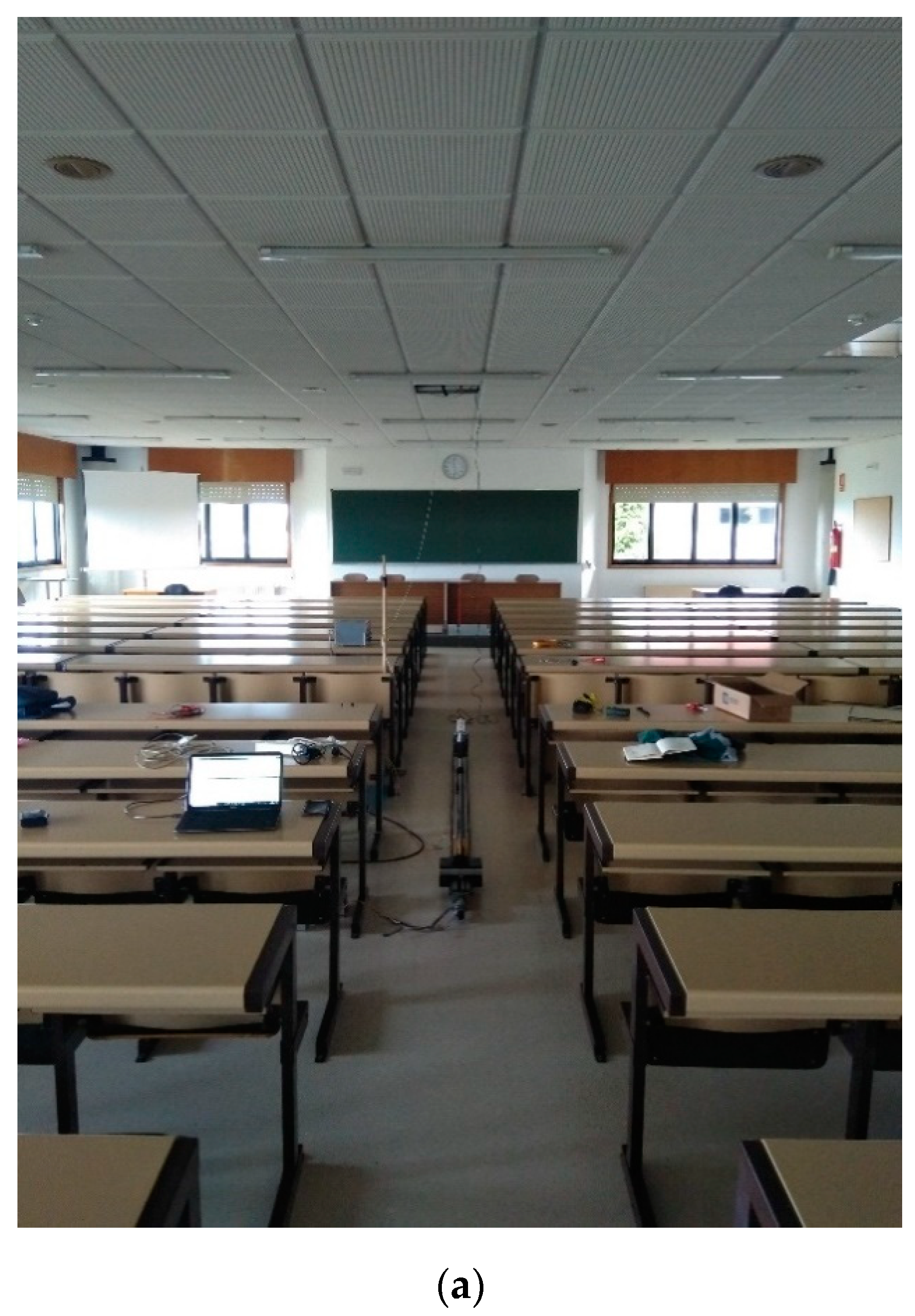
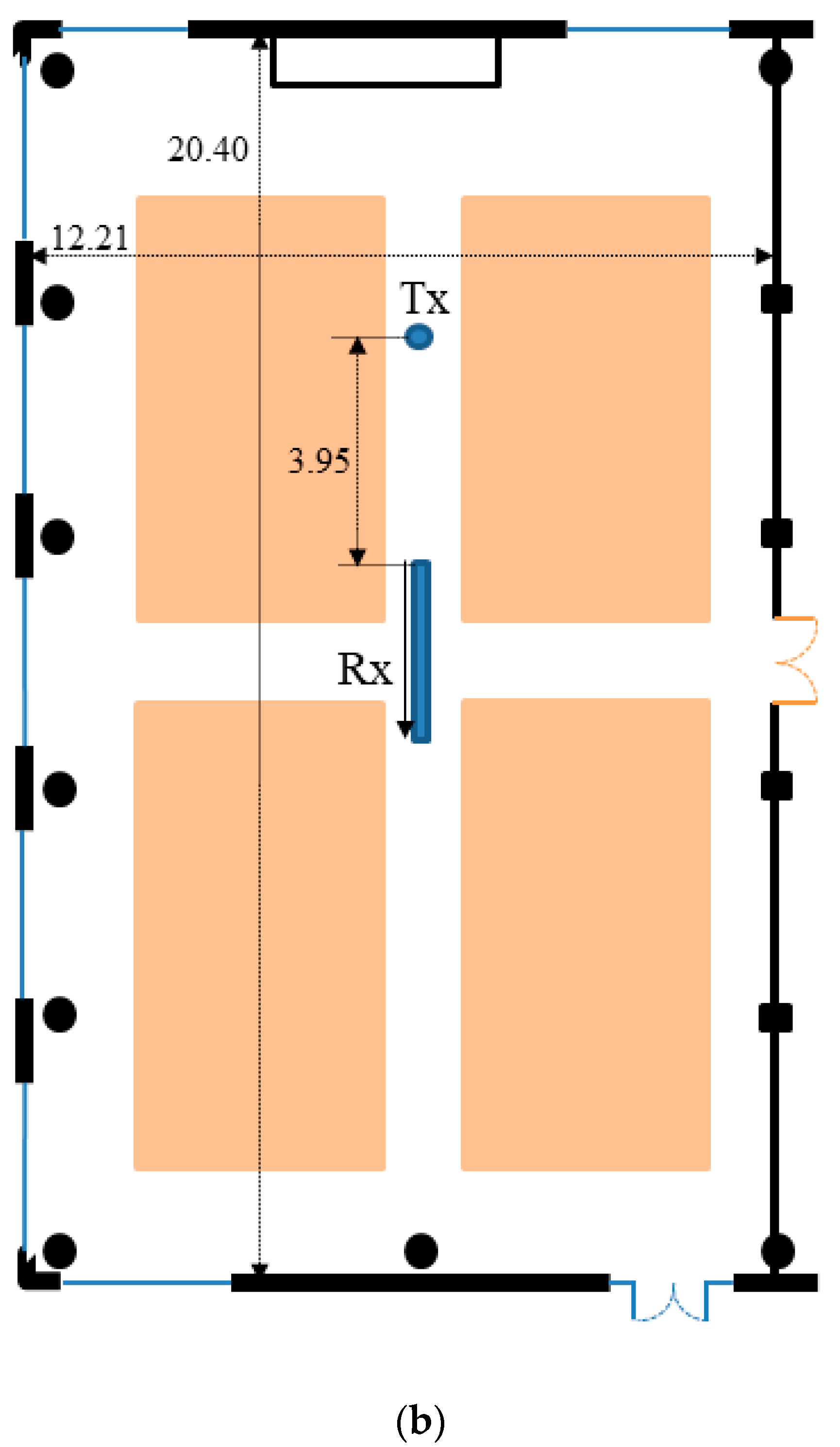
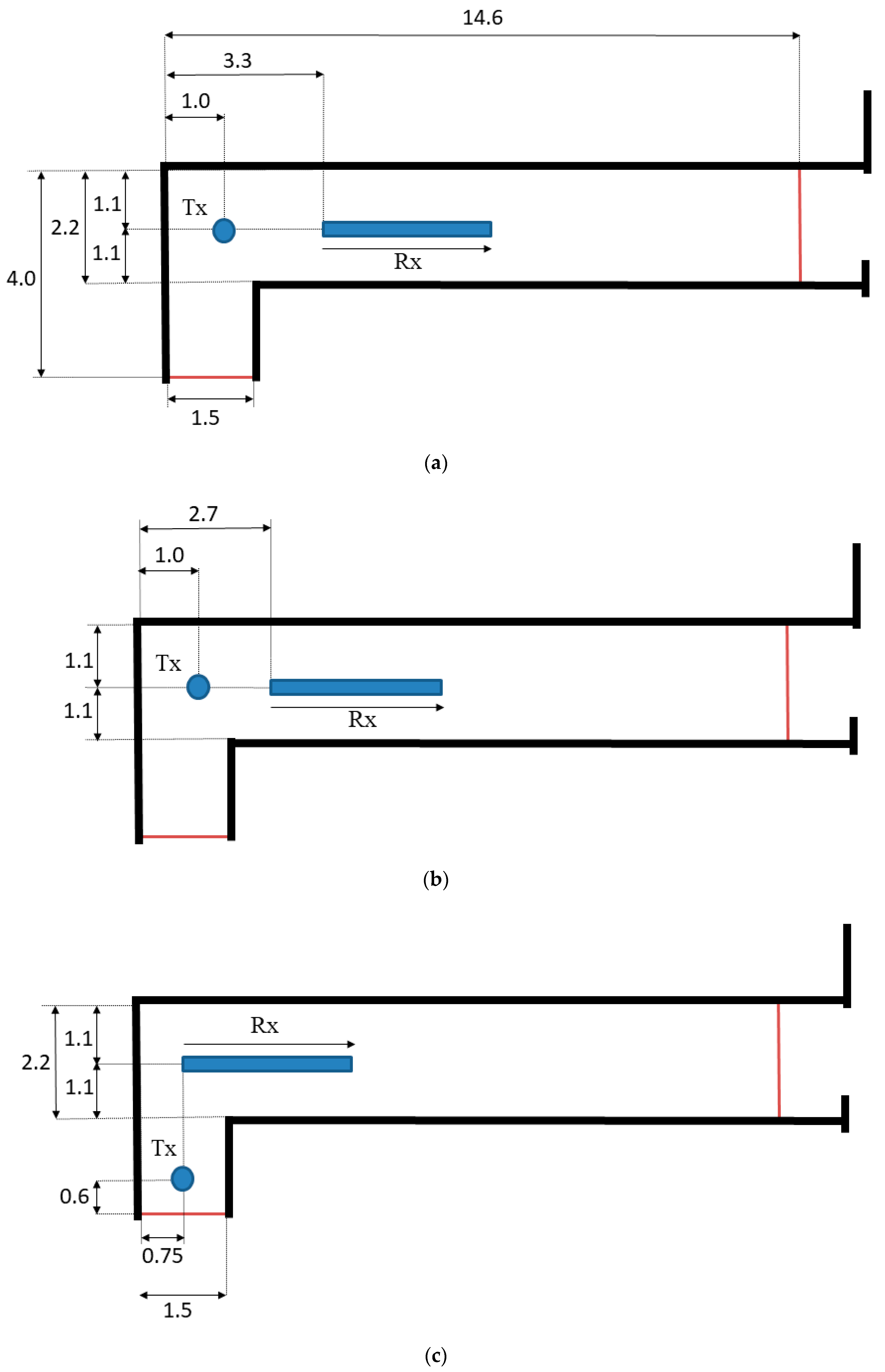
2.2. Measurement Environments

Measurements took place in two different scenarios: An ordinary auditorium used for teaching activities and a corridor, both at the School of Telecommunication Engineering at the University of Vigo. During measurements the presence of people moving within the environments was not allowed, only the antennas changed their position. This results in a static environment.
The auditorium is a flat classroom furnished with chairs and tables divided into four big blocks. It has a brick wall covered by plaster on one of the sides, while the opposite wall has plenty of large windows. At the back of the auditorium there is another wall with a couple of glass doors and windows. The last wall has a blackboard and some more windows. The transmitting antenna was located at the ceiling, near the front of the room, and the three receiver antennas were on the moving stand of the rail. Figure 3 depicts this first environment, including the location of transmitting antenna and the paths for the receiving antenna during measurements.
The second scenario is a narrow corridor, with brick walls covered by plaster. The floor plans are depicted in Figure 4. This scenario hosted two different environments: LOS and OLOS, depending on the location of the transmitting antenna and its visibility from the receiving ones. The receiving antenna paths were at the exact center of the 2.20-m width corridor, whereas the transmitting antenna location varied depending on the configured environment: For LOS the antenna was at the ceiling, also in the middle of the corridor; for the OLOS, a wall corner obstructed the line of sight between the antenna (again at the ceiling) and the receiving path. Figure 5 shows a picture taken during the measurements.

2.3. Data Processing

An inverse Fourier transform is applied to the measured complex frequency responses of the radio channel in order to obtain the channel impulse responses h(t,τ). Due to the limited frequency range of the measurements the frequency response is windowed and the impulse response may contain certain peaks originating from the side lobes of the window response in the time domain. To remove these peaks which do not correspond to actual propagation paths, as well as part of the noise, we set a threshold according to [6] and remove any sample below that threshold. Then we use those impulse responses to compute the power delay profile (PDP) as is shown in Equation (1) and represent the power received at a certain location as a function of the delay, τ [7,8].
P D P ( τ ) = 1 N n = 1 N | h ( τ , n · Δ l ) | 2
where Δl is the step distance the receiver antennas are moved between successive measurements.
As seen in Equation (1), there is an averaging process of N impulse responses to obtain the PDP. We used a sliding average with N = 11 to obtain the results of this paper [7]. Based on the PDP vectors some relevant time dispersion parameters were computed: The mean delay and the RMS delay spread. The mean delay is the first moment of the power delay profile, and it is defined as in Equation (2).
τ m e a n = k = 0 P D P ( τ k ) τ k k = 0 P D P ( τ k )
The RMS delay spread is even more interesting than the mean delay, as it is related to the inter-symbol interference (ISI) phenomenon giving cause to the irreducible bit error rate (BER) of the radio communication system. The RMS delay spread is the standard deviation of the delay of multipath components, weighted proportional to the energy transported by each of them. This RMS delay spread is also the square root of the second central moment of the PDP. The formula for the RMS delay spread is shown in Equation (3) [8,9]. The symbol interval used in the system has to be much larger than the RMS delay spread of the radio channel to avoid ISI [10].
τ r m s = k = 0 ( τ k τ m e a n ) 2 P D P ( τ k ) k = 0 P D P ( τ k )
Both time dispersion and frequency selectivity are important factors when dealing with multipath channels. The most commonly used parameter to express frequency selectivity is the coherence bandwidth (Bc). This bandwidth is a statistical parameter, and can be defined as that part of the bandwidth where the channel response is considered flat. In other words, it represents the range of frequencies that experience correlated fading [11,12].
Computing the frequency correlation function (FCF or ) is the first step to calculate the coherence bandwidth, Bc. The frequency correlation function is the Fourier transform of the PDP, as indicated in Equation (4). Typical values of the correlation level (α) used to estimate Bc are 0.5, 0.7 and 0.9. The Bc is then that part of the frequency range where the FCF is above one of these levels [8,11,12].
R τ ( Δ f ) = P D P ( τ ) e j 2 π Δ f τ d τ
Figure 6 depicts the estimation of coherence bandwidth at those correlation levels on the computed frequency correlation function for the auditorium at 40 GHz and received by antenna “3”. The coherence bandwidths at which the frequency correlation function is above 0.9, 0.7 and 0.5, are, respectively 24 MHz, 138 MHz and 222 MHz.

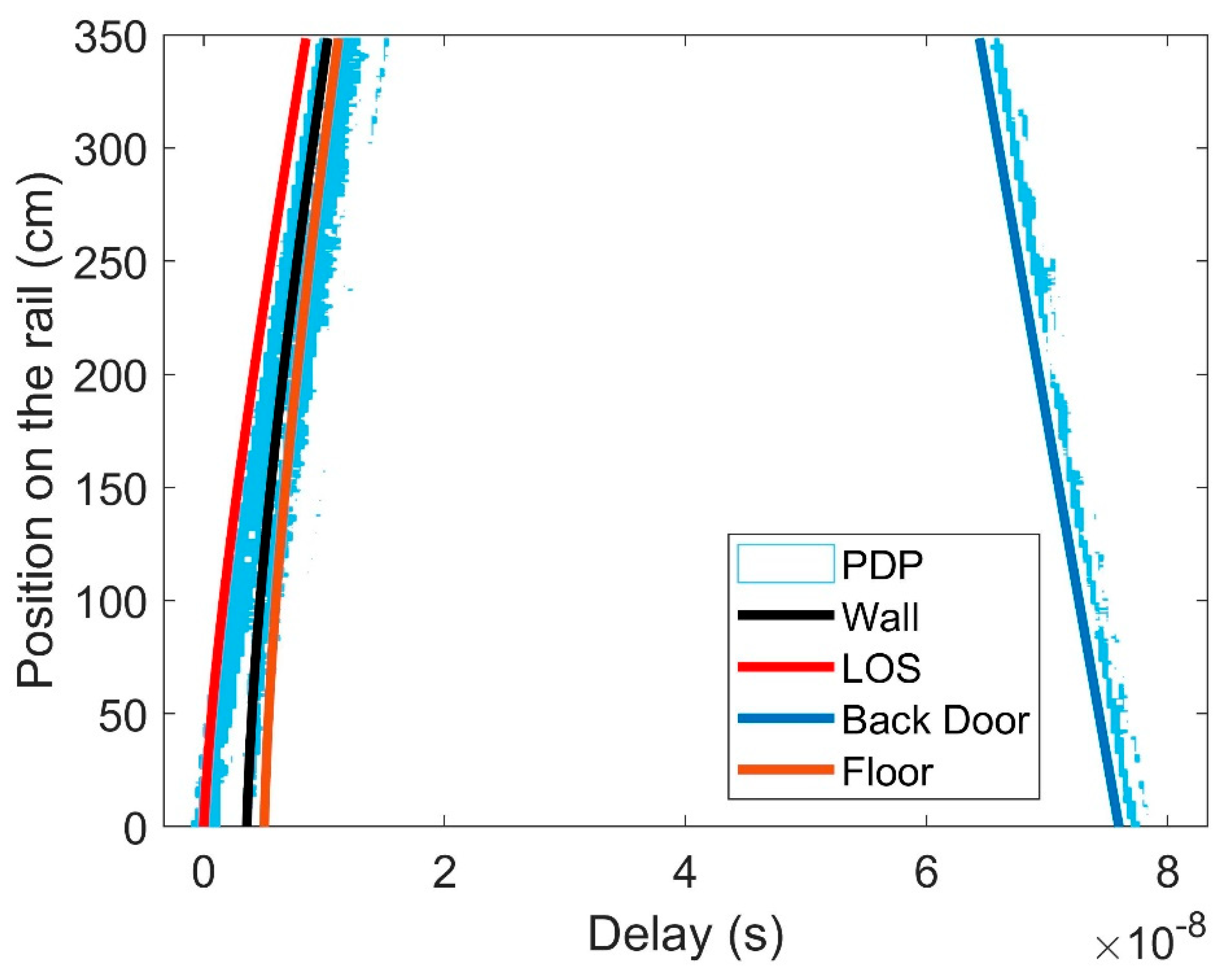
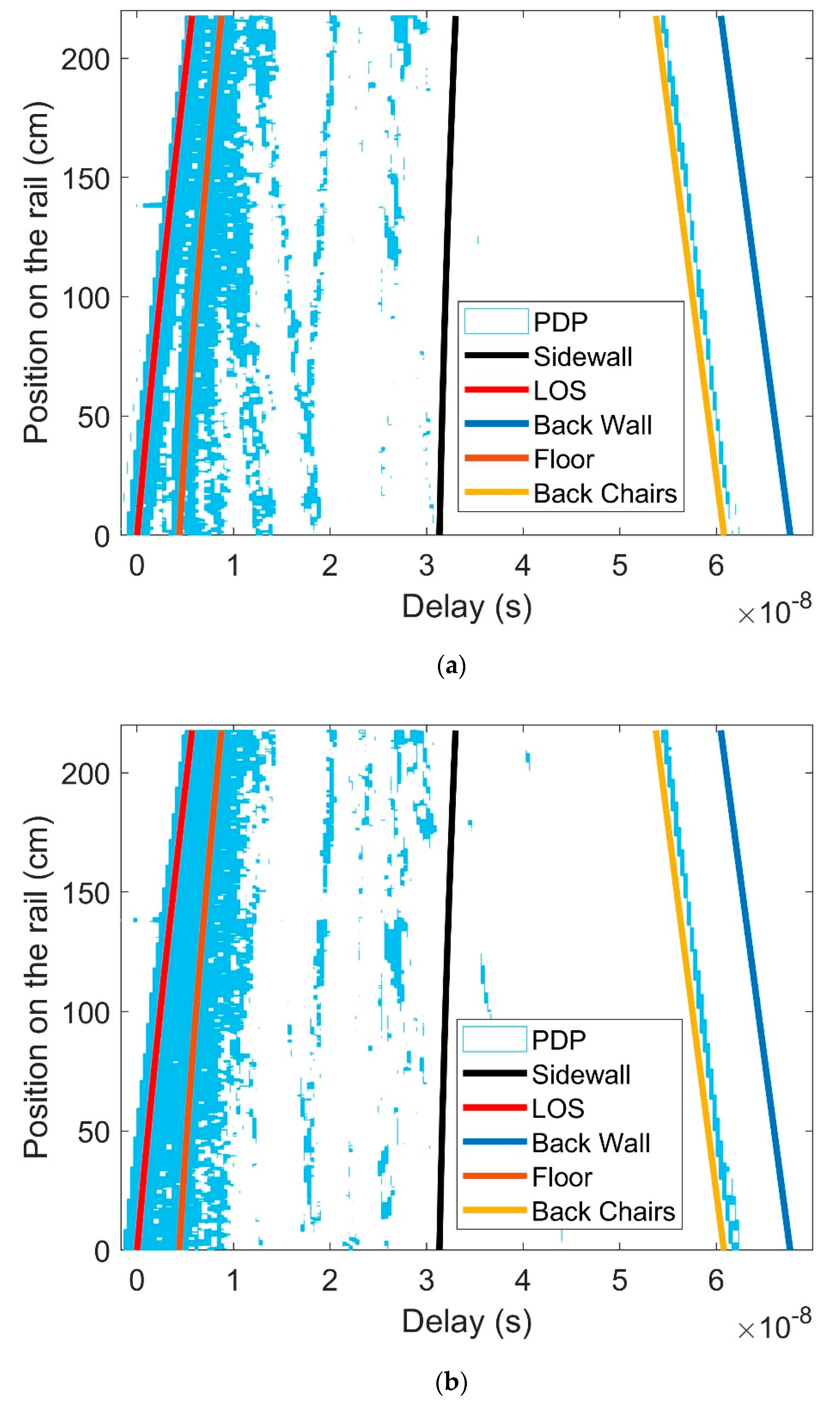
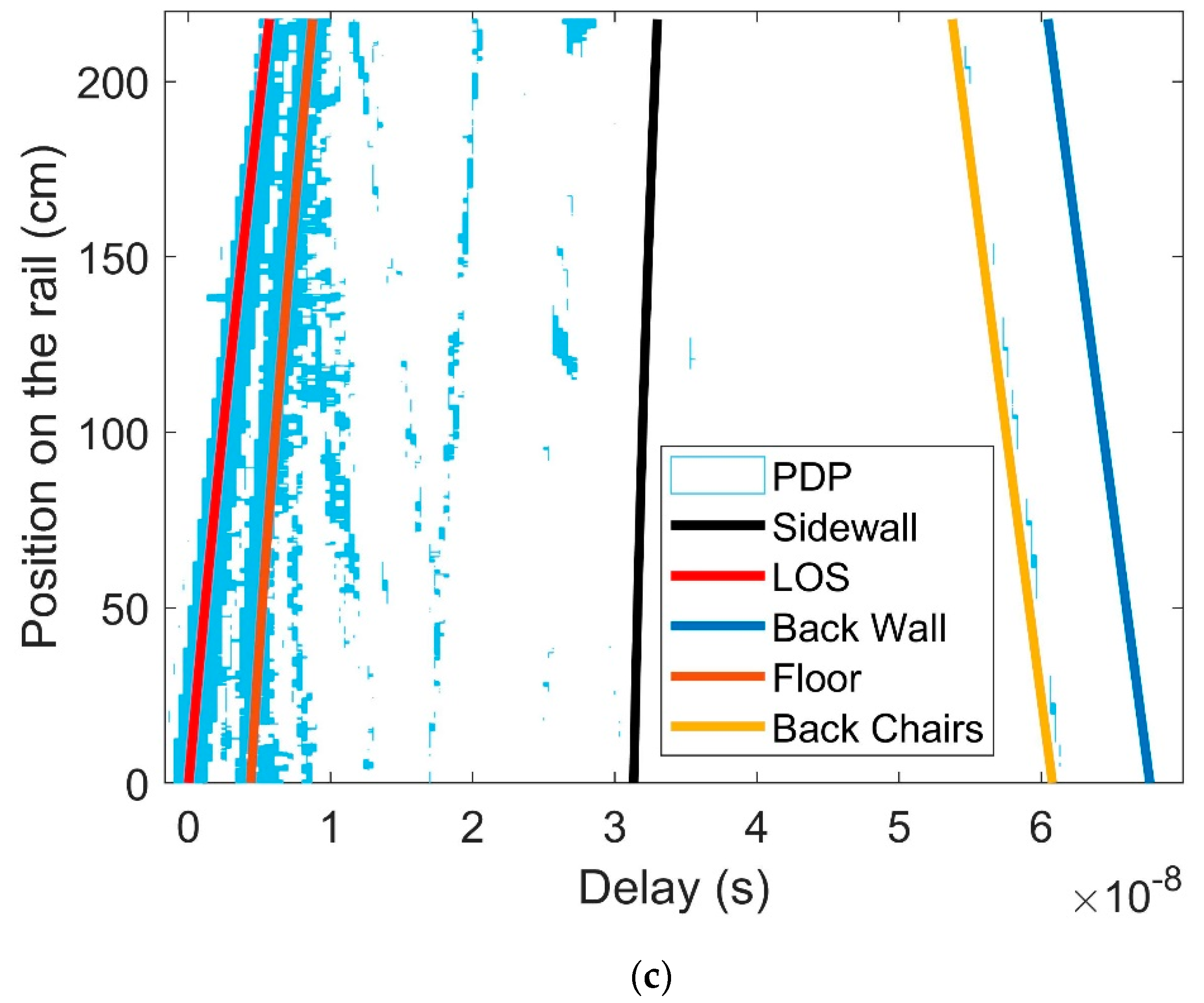
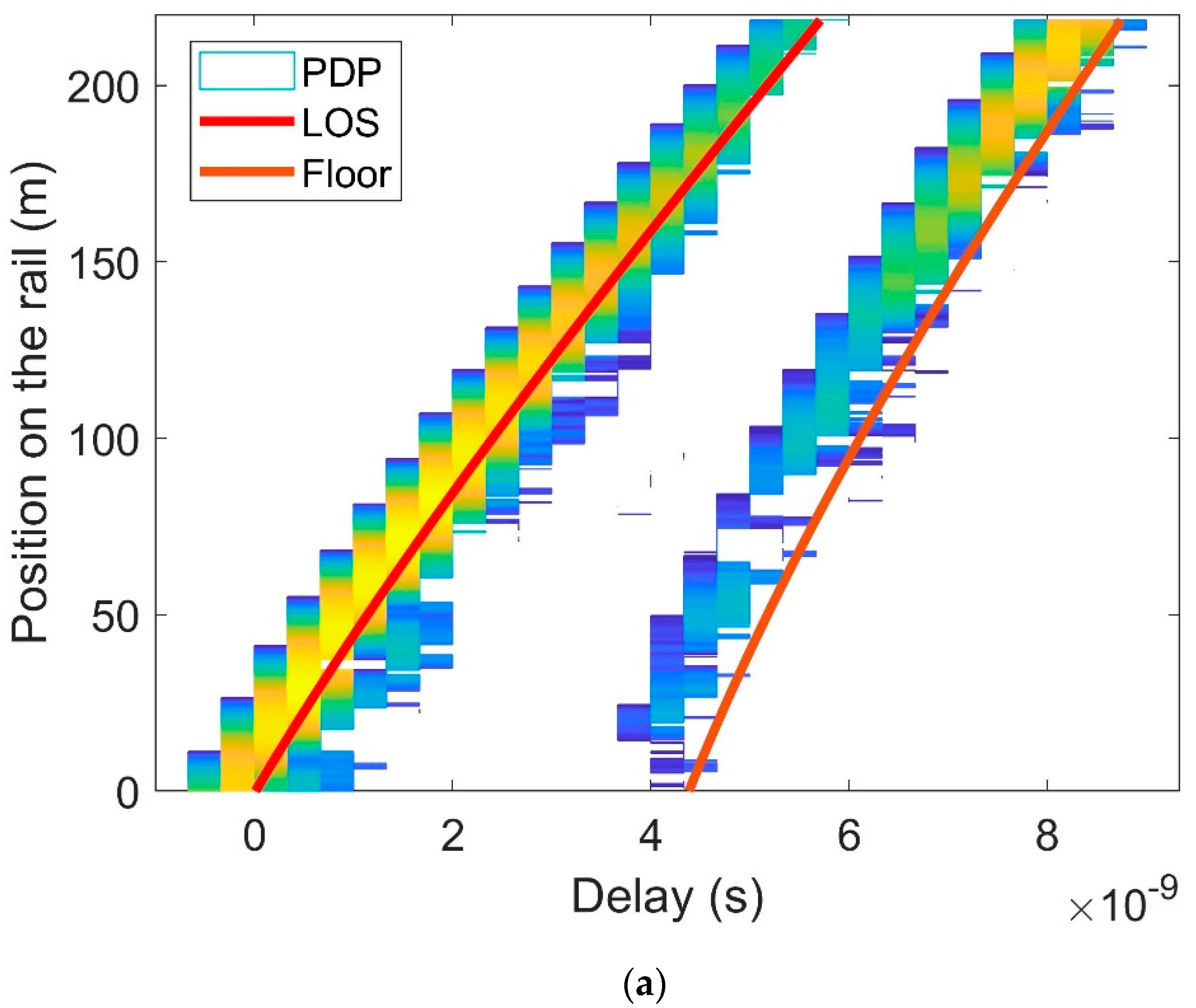
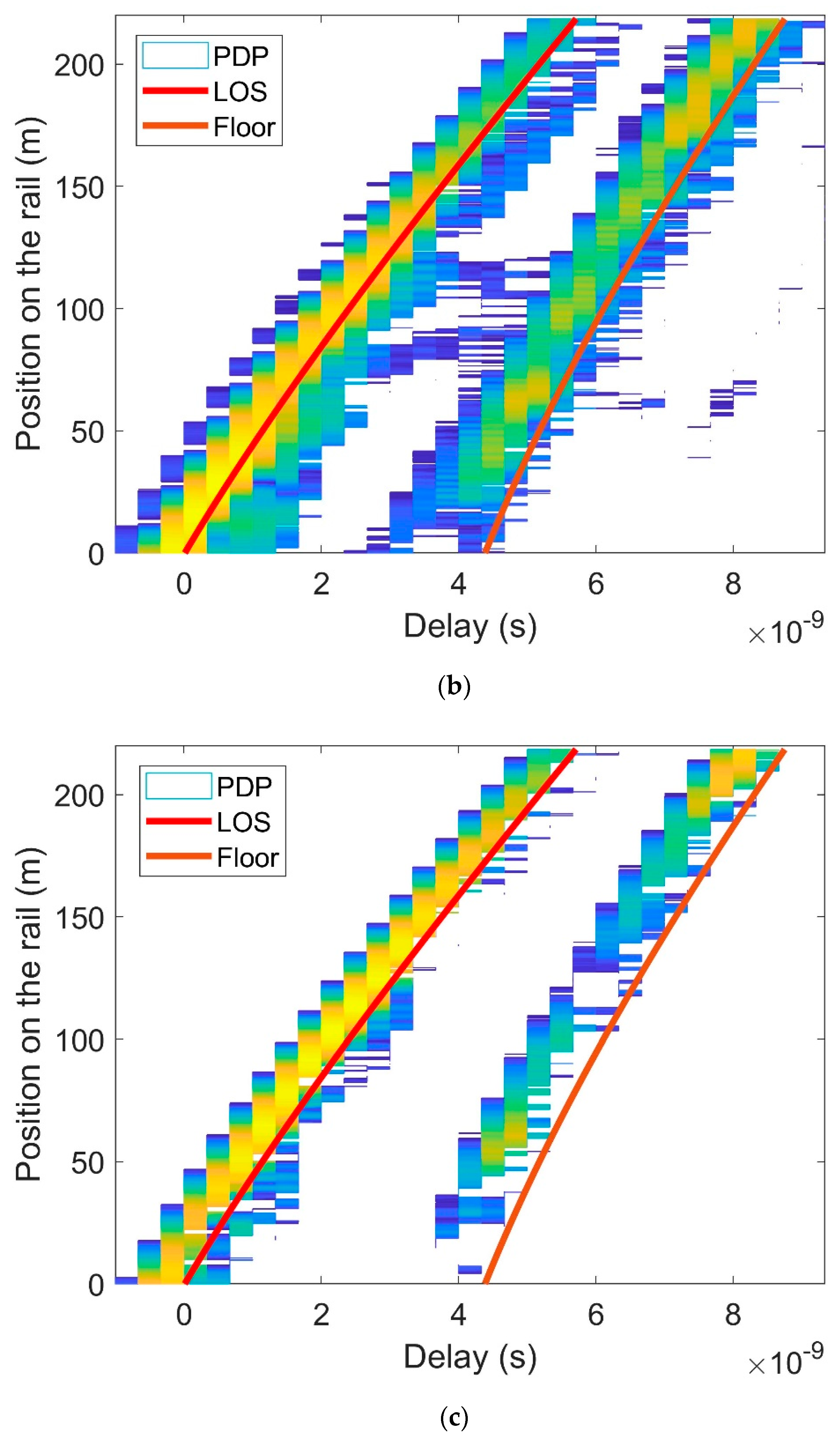
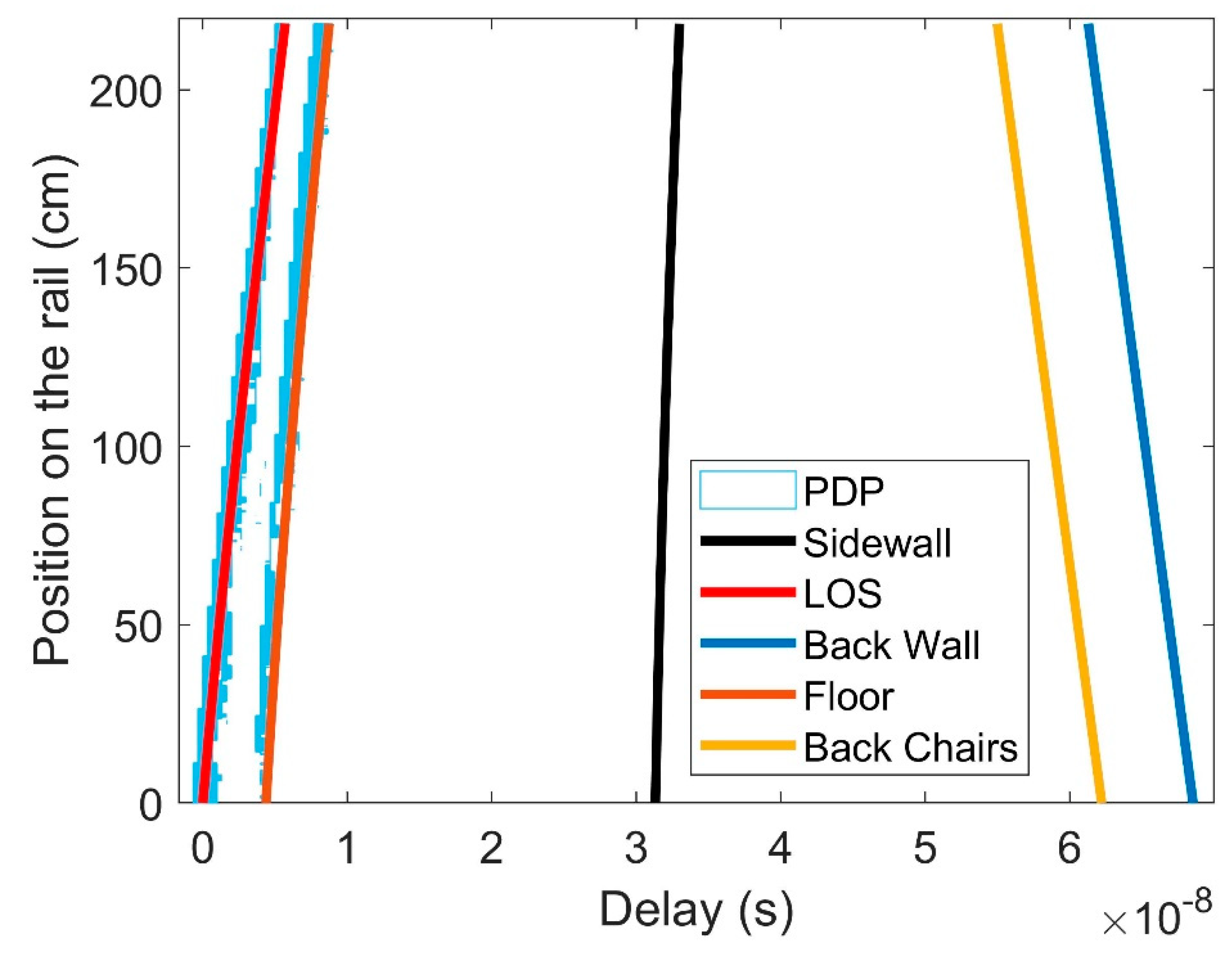
2.4. Ray-Tracing Analysis

The time difference in the various echoes relative to the first arriving component (the one corresponding to the direct path in an LOS situation) can give some information about where they have been produced. Multipath components in the PDP are associated with a certain delay and thus with a certain travelled distance. Using these delays and the dimensions and geometry of the environment, each multipath component can be mapped to a certain scattering element in the environment, wherefore a very simple ray-tracing tool has been developed only calculating the origin of the different multipath components and not the amplitude of them. Using image theory [13], first order reflections on the most significant elements were computed.
Figure 7 shows, as an example, the fit between the PDP obtained from measurements and the delay of different propagation paths computed by the above-described ray-tracing tool. Up to four different paths considered by the ray-tracing tool superimpose to the measured PDP, whereas the LOS component and the floor reflection fit perfectly the empirical results, the reflection caused by the back door seems just a bit ahead of the measured one. This may be due to small measurement errors, a more complex multipath propagation than that used in the simulations, or even some additional delaying elements not considered in this analysis.

3. Results

In this section, results obtained in the auditorium and the corridor, are presented. Every measurement results in three different S-parameters, measured at the same time, which allows observing the difference between multipath components arriving at the three antennas. All wideband results are shown, relative to the delay of the main LOS component.

3.1. Auditorium

Figure 8a–c show the PDP for the three S-parameters at 41.5 GHz. Taking a closer look at the area of the component arriving first, it is easy to see that antenna “2” (closest to the transmitter) gets the most energy of the three. This can be explained by the fact that also reflections from the floor, tables and chairs are taken together, where those are at the same time partially blocked to the other antennas. Another explanation can be the coupling of the different receiving antennas, resulting in (smaller) modifications of the radiation pattern and hence reducing efficiency and performance.
The direct component can be easily identified as the one with the smallest delay. As the receivers move away from the transmitter, that relative delay increases. The same trend can be seen in other contributions produced by scatterers placed between the transmitter and the receivers.
However, at the central part of the graphs, there is a contribution that can be seen in Figure 8a (and less clearly in Figure 8c) starting at 20 ns delay and lowering its delay as the receivers move away from the transmitter. This indicates that the contribution is arriving from a direction opposite to that of the direct component. It was probably produced by the laptop, which was the closest to antenna “2”.
As our simple ray-tracing tool does not take into account the amplitude of the components, it could predict some components that do not appear in the actual measured results due to their large attenuation and low power in the real world. This is the case for the sidewall reflection in Figure 8.
Finally, the contributions coming from the chairs at the back area of the auditorium can also be identified by their initially longer delays, getting shorter when the receiver moves closer to these scatterers.
Figure 9 shows the measured PDP at the 60 GHz band together with the ray-tracing predictions. Aside from the difference between the three receivers, it is also interesting to recall the differences on the PDP between 40 GHz and 60 GHz. While for 40 GHz there are several multipath components, in 60 GHz only the line of sight and the reflection on the floor are present. The other contributions from the side and back wall suffer stronger attenuations and fall below the receiver’s sensitivity (Figure 9a–c). In fact, the ray-tracing simulations predict the time delays that would correspond to those contributions, as can be seen in Figure 10, but no signal over the noise threshold was detected in the measurements.
As stated before, time dispersion affects the maximum symbol rate that can be used without suffering ISI. In Figure 11, the RMS delay spread for all three S-parameters at both frequencies is plotted as a function of the receiver’s position. The results are consistent with what was shown before (Figure 8 and Figure 9). At 40 GHz the amount of multipath is more significant than at 60 GHz; therefore, the RMS delay spread is also larger.
Another interesting way to analyze the RMS delay spread values is by means of their cumulative distribution functions (CDFs). Computing the CDFs of the RMS delay spread can help to establish a reference value for the delay spread in that environment, by setting a level below which it stays for 99 percent of the time.
Taking a closer look at Table 1, it shows that the most restrictive antenna (the one with the larger value of RMS delay) is antenna “3”, which is the one at the front. Hence the system must be designed to take that value into account. Again, the lower delay spread at 60 GHz, when compared to 40 GHz, is obvious in Table 1.
The second computed parameter is the coherence bandwidth. At 40 GHz, the results are very similar for all three antennas, as can be seen in Figure 12. For the signal received by antenna “2” and “4” similar behavior is observed: A level of about 800 MHz for α = 0.5 until the antennas are moved 100 cm on the rail. The reason for this large coherence bandwidth is that at short distances the main contribution is the direct one, while the ground reflection is attenuated by the antenna pattern (as seen in Figure 9). As the distance increases, the ground reflected component is received through the center of the main lobe of the antenna pattern, and the coherence bandwidth decreases drastically. Comparing those results with the ones obtained by antenna “3”, the level of the coherence bandwidth in the latter is smaller and the decay is produced at a closer distance to the transmitter.
When looking at the results for 60 GHz in Figure 13, one can observe the increase in the mean level of the coherence bandwidth for all correlation levels. This can be explained by the reduced number of echoes, compared to the 40 GHz frequency campaign.
As with the RMS delay, the percentage of the time the coherence bandwidth is above a desired threshold and is a useful metric for the design of communication systems. Here, the results for the 99th percentile can be seen in Table 2.
We can observe that for a coherence level of 0.9, 60 GHz clearly outperforms 40 GHz. For lower correlation levels, that behavior is not that clear. In addition, for both frequency bands, the worst scenarios are given when receiving through antenna “3”.
Comparing the coherence bandwidth and the RMS delay spread values, it is clear that there is an inverse relation. The more replicas of the signal received, the larger the RMS delay spread and the lower the coherence bandwidth become. The mathematical relation is given by Fleury’s limit [14,15] in Equation (5).
B c cos 1 α 2 π τ r m s
where Bc is the coherence bandwidth for a correlation level α and τrms is the RMS delay spread.
Figure 14 illustrates both theoretical lower limits for the coherence bandwidth with different correlations and the results obtained by analyzing the available data and plotting them as a function of RMS delay at 60 GHz.

3.2. Corridor

Wideband results obtained in the corridor, in both LOS and OLOS, were processed in a similar way. Table 3 and Table 4 provide RMS delay spread values and Table 5 and Table 6 coherence bandwidth values, for LOS and OLOS conditions.
Observing Table 3 and Table 4, one can notice a clear difference between 40 GHz and 60 GHz. Both in LOS and OLOS, the 60 GHz signals demonstrate a lower delay spread. Indeed, the lower the frequency the more multipath is observed in the measurement campaign. Obviously, the multipath scheme is the same in both environments. However, the attenuation at 60 GHz is stronger than at 40 GHz as many multipath components at 60 GHz arrive at the receiver with a level below its sensitivity, and hence do not contribute to the received signal. Less multipath components result in a lower RMS delay spread.
The difference in RMS delay spread between LOS and OLOS is clear at 60 GHz, with lower values in LOS and with a stronger dominant direct path than in OLOS. The difference is not so clear at 40 GHz.
In general, the coherence bandwidth in these corridor scenarios is higher in the first part of the rail. After a certain distance, it drops to nearly half its value. The drop appears around 130 cm for 60 GHz and 150 cm for 40 GHz. There are two explanations for this behavior. The first one is that the antenna quits the main lobe, resulting in a weaker value in the PDP. The second one is that the multipath components are reduced, due to the environment geometry.
In the LOS scenario, the coherence bandwidth is higher at 40 GHz than at 60 GHz, as can be seen in Table 5. As previously stated, this is expected due to the higher amount of multipath. In OLOS (Table 6) the 60 GHz seems to be higher, but this is due to the absence of received signal at some places along the path.
Regarding the theoretical limits for the coherence bandwidth, Figure 15 shows the Fleury’s limit for the case of the measurements in the 40 GHz band at the corridor.

4. Discussion

Throughout the paper, several results provide insight into the behavior of the indoor radio channel at different environments in two clearly different millimeter-wave frequency bands: The licensed one near 40 GHz and the unlicensed around 60 GHz. Their characteristics allow the definition of advantages and disadvantages of both for deploying high rate wireless networks, which is the aim of this work.
From the measurement data and the processing of this gathered information, the main observed differences are:
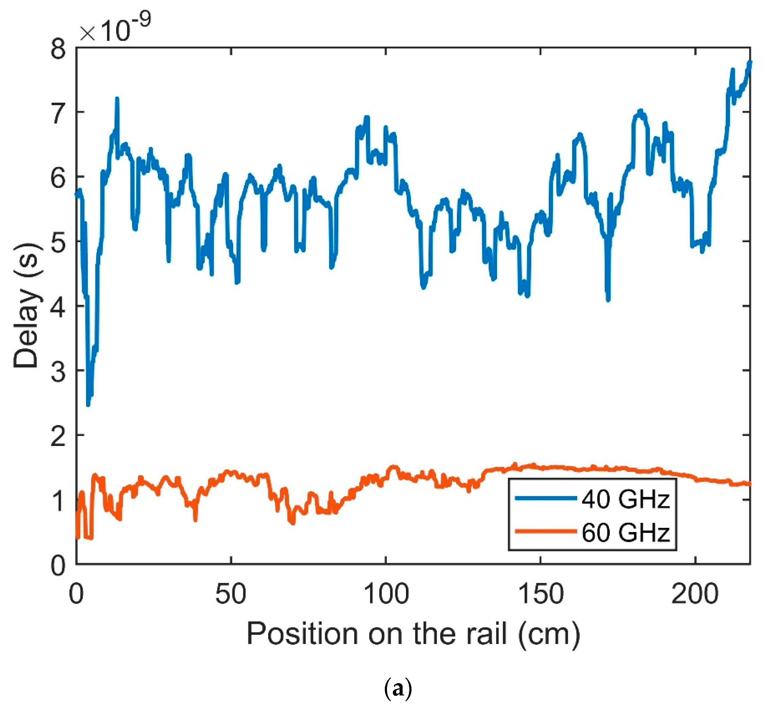
  • The amount of multipath contributions is clearly reduced in 60 GHz compared to 40 GHz. This is due to the larger propagation attenuation and lower reflection coefficients at 60 GHz. At 60 GHz the energy will be scattered in a more diffuse way as the wavelength is smaller compared to the surface irregularities.
  • This leads to smaller delay spreads at 60 GHz than at 40 GHz (i.e., 2.73 ns versus 8.64 ns at the auditorium).
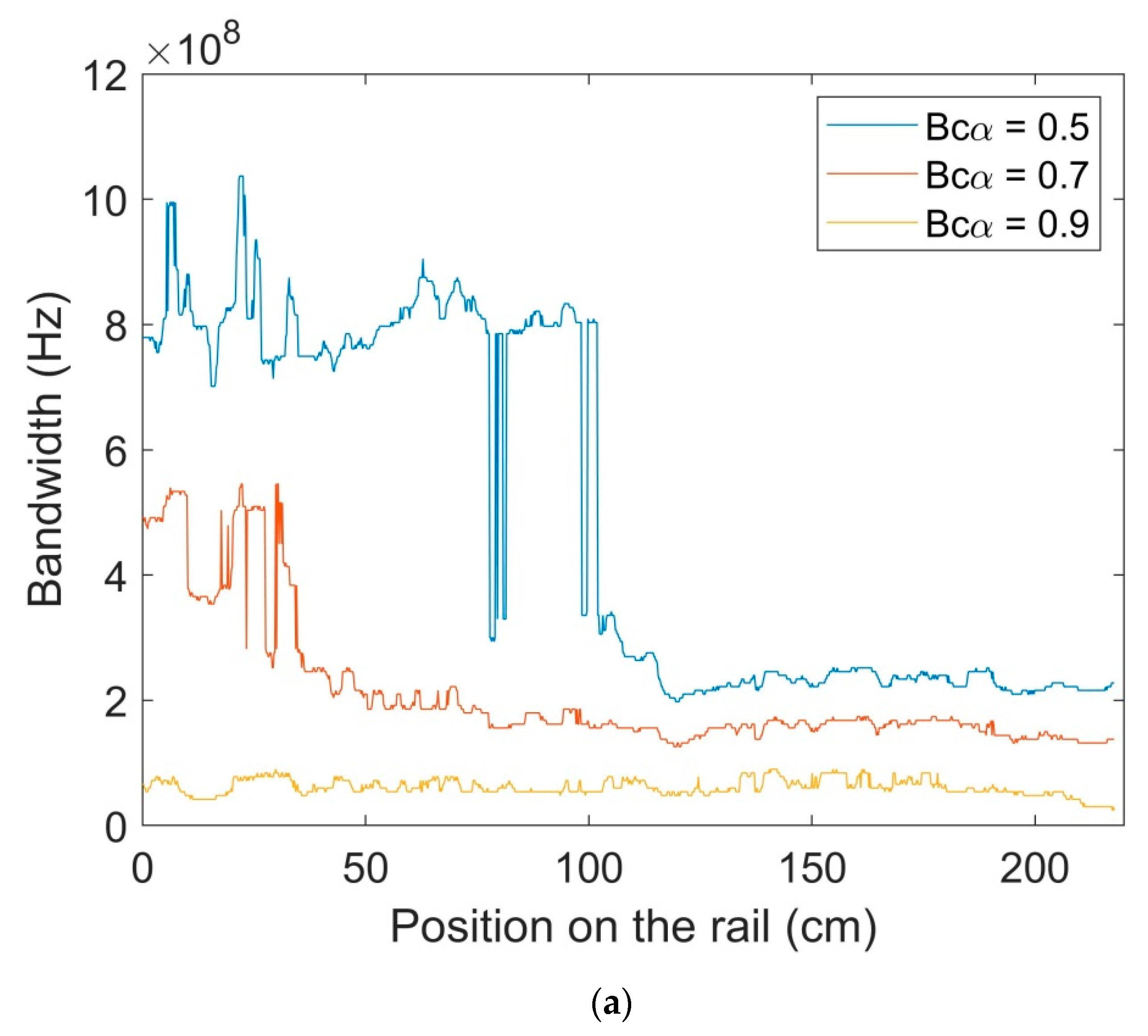
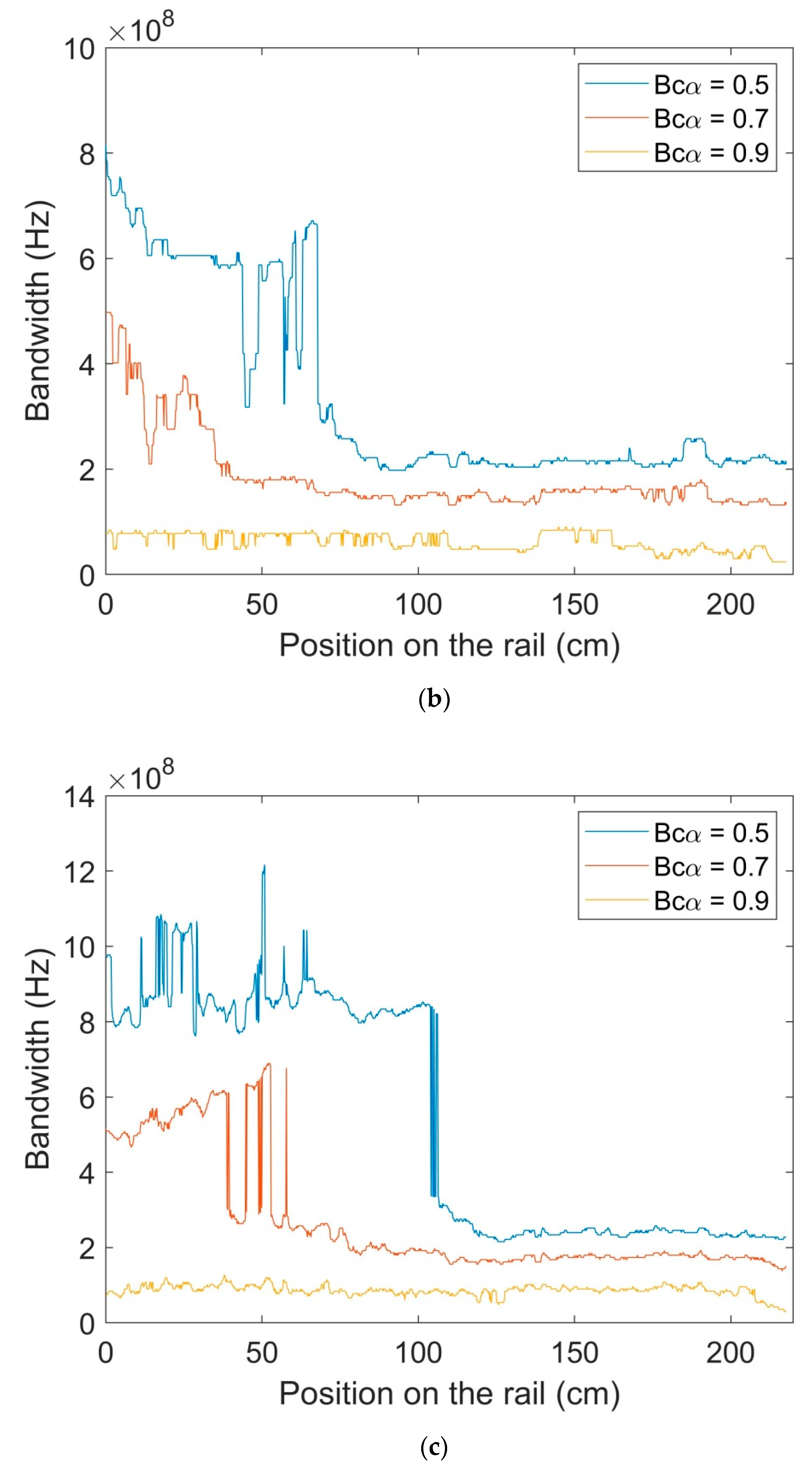
  • The radio channel is more frequency selective at 40 GHz, with coherence bandwidths for a 0.9 correlation level of 24 MHz at 40 GHz in the auditorium, while a value of 78 MHz was measured in the same environment at 60 GHz.
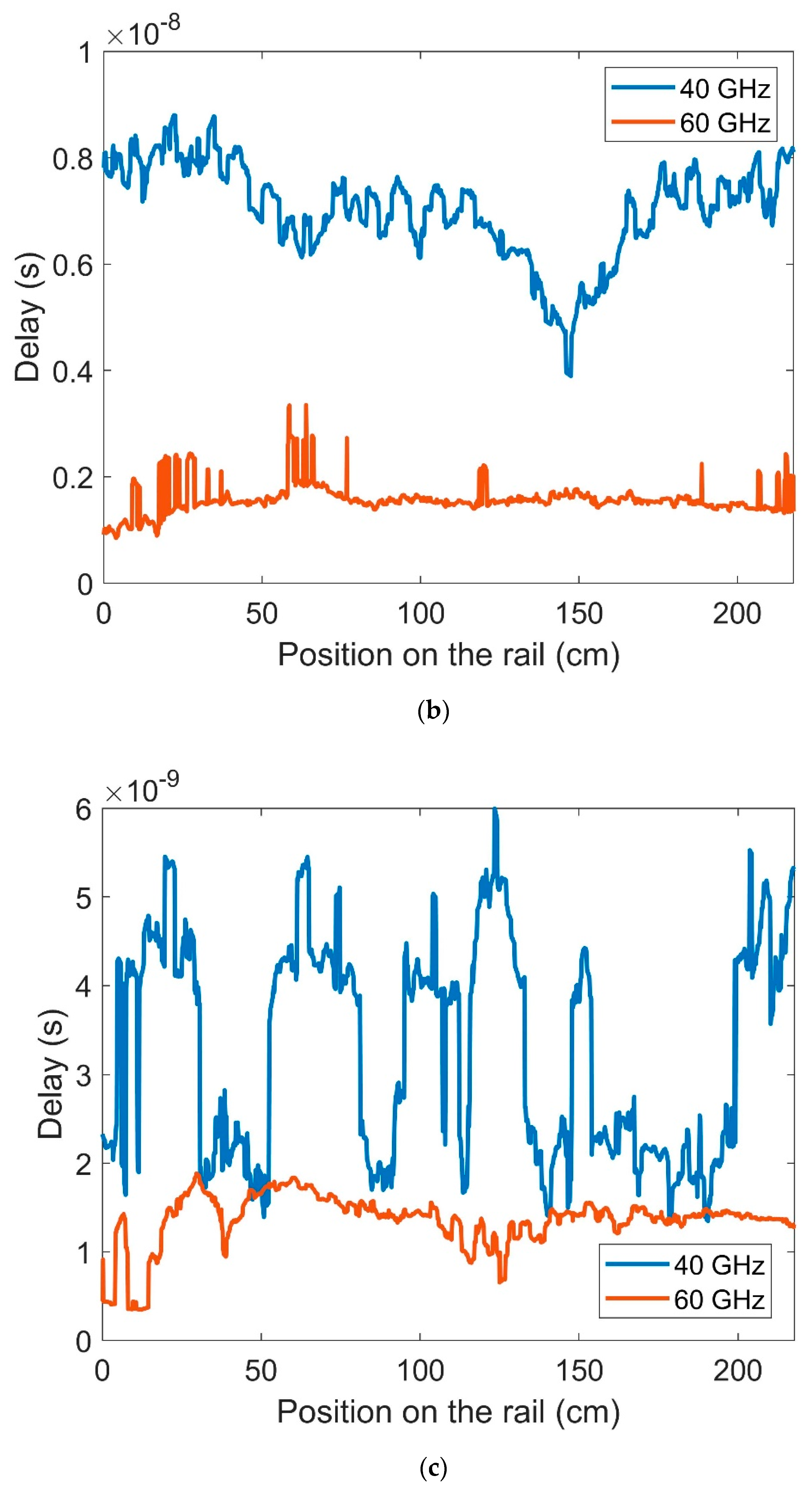
  • Regarding the different scenarios in LOS conditions, smaller environment dimensions yield to a smaller RMS delay spread at 60 GHz. A value of 0.1 ns is obtained in the corridor while 2.73 ns is obtained in the auditorium. At 40 GHz the difference is not so clear (8.4 ns versus 8.64 ns).
  • On the other hand, smaller scenarios correspond to larger coherence bandwidth values, particularly at 60 GHz, with coherence bandwidth values for a 0.9 correlation level increasing from 6 MHz in the corridor to 78 MHz in the auditorium.
  • OLOS conditions result in larger delay spreads (5.1 ns) compared to LOS conditions (0.1 ns) at 60 GHz. The difference at 40 GHz is no so clear (8.7 ns versus 8.4 ns).
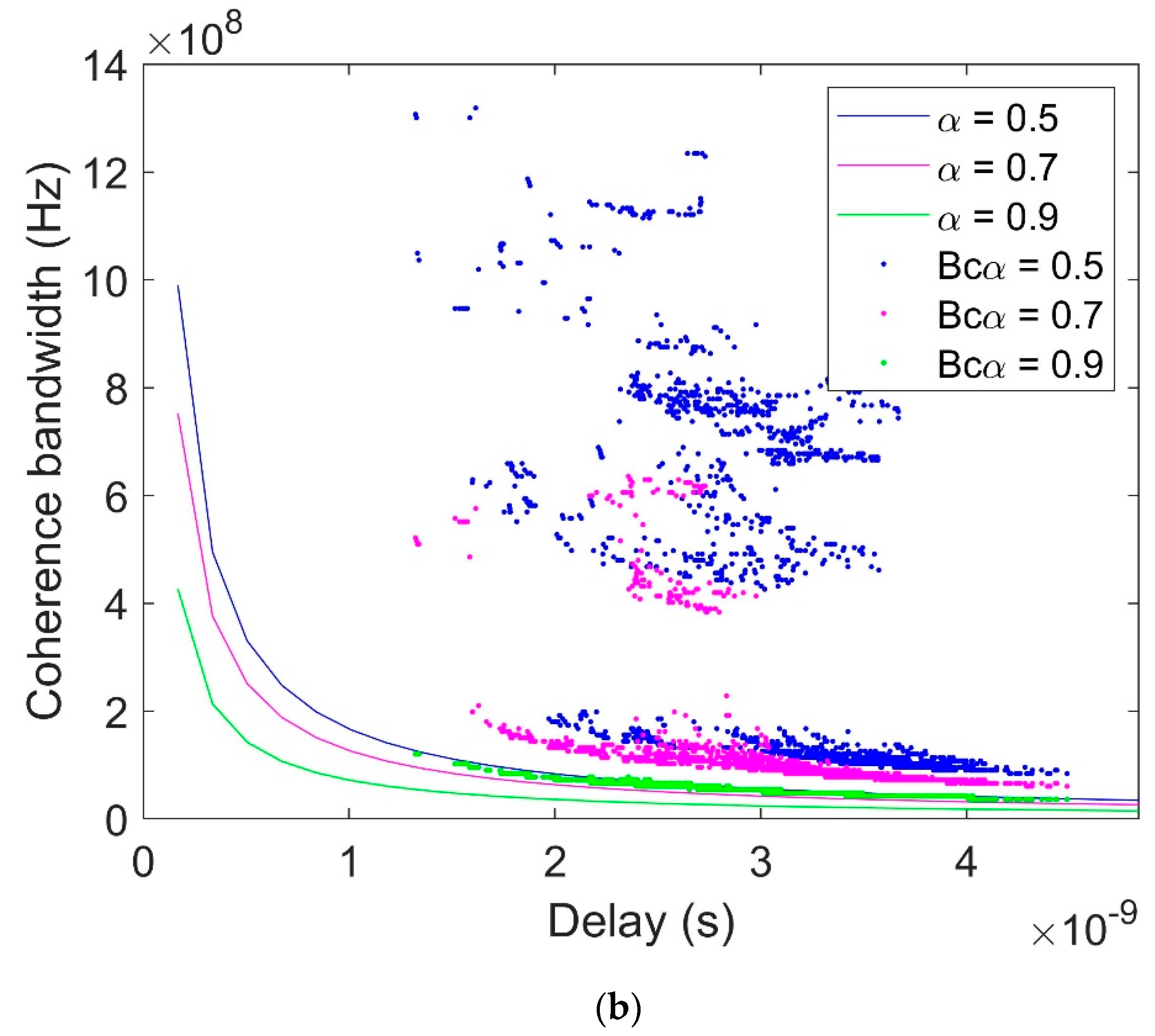
  • The inverse relation between the delay spread and coherence bandwidth has been confirmed by plotting both parameters against Fleury’s limit.
  • Due to the reduced multipath propagation conditions at 60 GHz, channel parameters seem to be more sensitive to changes in the size of the environment and on the visibility conditions (LOS/OLOS) than at 40 GHz.
  • Regarding ray-tracing simulations, a simple ray-tracing model with just single reflections would be enough to represent all relevant multipath contributions at 60 GHz. Higher order reflections should be considered for modelling all contributions at 40 GHz.
At 38 GHz, results for the corridor agree with those in the literature [16] where measurements were performed in a wagon with similar dimensions and geometry. The delay spread values reported are 7.63 ns and 9.77 ns, very similar to the 8.4 ns we measured in LOS condition.
At 60 GHz, similar delay spread values can be found in [17] where a mean delay spread value of 6 ns with 2 ns standard deviation are reported for a conference room and in [18] where delay spreads below 7 ns are measured for 99% of the positions, also at a similar conference room. Finally, in [19] a value of 3.13 ns is found, but for a smaller environment.

5. Conclusions

A wideband measurement campaign at two millimeter-wave frequency bands, 40 GHz and 60 GHz, has been conducted in two indoor scenarios: An auditorium and a narrow corridor. Measurements included both LOS and OLOS situations.
The results have been processed and two wideband channel parameters have been obtained: The RMS delay spread and the coherence bandwidth. Based on these two parameters, the performance of both frequency bands is compared.
We conclude that there are more multipath contributions at 40 GHz than at 60 GHz, resulting in a larger delay spread and larger frequency selectivity at 40 GHz than at 60 GHz. The radio channel at 60 GHz seems to be more sensitive to any change in the size of the environment or in the visibility conditions (LOS/OLOS).
We have also concluded that multipath contributions at 60 GHz can be explained by single reflections on the environment scatterers, while higher order reflections should be considered to model all multipath contributions at 40 GHz.
The results in this paper should be taken into account if a decision has to be made on the frequency band to be used in an indoor link for a wireless communication system. Results also provide a deep insight into the physical propagation mechanisms that take place and help to understand how these mechanisms determine the differences in the wideband parameters of the radio channel. Finally, results will be valuable also for those developing ray-tracing models for the indoor radio channel at millimeter-wave frequencies.

Author Contributions

Design of the measurement campaign M.G.S. and I.C.; measurement system setup, measurements and data processing: R.H. and M.R.; analysis of results: M.G.S., I.C. and J.V.; writing: all.

Funding

This research was funded by the Spanish Government, Ministerio de Ciencia, Innovación y Universidades, Secretaría de Estado de Investigación, Desarrollo e Innovación, grant number TEC2017-85529-C3-3R); Xunta de Galicia, grant number ED431C 2019/26; atlanTTic Research Center; and the European Regional Development Fund (ERDF).

Acknowledgments

The authors would like to thank Isabel Expósito for her technical support in the management of the radioelectric equipment.

Conflicts of Interest

The authors declare no conflict of interest.

References

  1. Marcus, M.J. 5G and “IMT for 2020 and beyond” [Spectrum Policy and Regulatory Issues]. IEEE Wirel. Commun. 2015, 22, 2–3. [Google Scholar] [CrossRef]
  2. Rappaport, T.S.; Sun, S.; Mayzus, R.; Zhao, H.; Azar, Y.; Wang, K.; Wong, G.N.; Schulz, J.K.; Samimi, M.; Gutierrez, F. Millimeter Wave Mobile Communications for 5G Cellular: It Will Work! IEEE Access 2013, 1, 335–349. [Google Scholar] [CrossRef]
  3. European 5G Observatory “US 5G Auction, in the 24 GHz Band”. Available online: http://5gobservatory.eu/us-5g-auction-in-the-24-ghz-band/ (accessed on 21 September 2019).
  4. ITU-R Recommendation M.2003-1. Multiple Gigabit Wireless Systems in Frequencies around 60 GHz; Recommendation: Geneva, Switzerland, 2015. [Google Scholar]
  5. Pahlavan, K.; Howard, S.J. Frequency domain measurements of indoor radio channels. Electron. Lett. 1989, 25, 1645–1647. [Google Scholar] [CrossRef]
  6. Varela, M.S.; Sánchez, M.G. An improved method to process measured radio-channel impulse responses. Microw. Opt. Technol. Lett. 2000, 24, 158–162. [Google Scholar] [CrossRef]
  7. Ai, B.; Guan, K.; He, R.-S.; Li, J.-Z.; Li, G.-K.; He, D.; Zhong, Z.-D.; Huq, K.M.S. On Indoor Millimeter Wave Massive MIMO Channels: Measurement and Simulation. IEEE J. Sel. Areas Commun. 2017, 35, 1678–1690. [Google Scholar] [CrossRef]
  8. Cuiñas, I.; Sanchez, M.G. Measuring, modeling, and characterizing of indoor radio channel at 5.8 GHz. IEEE Trans. Veh. Technol. 2001, 50, 526–535. [Google Scholar] [CrossRef]
  9. Zahedi, Y.; Ngah, R.; Nunoo, S.; Mokayef, M.; Alavi, S.; Amiri, I.S. Experimental measurement and statistical analysis of the RMS delay spread in time-varying ultra-wideband communication channel. Measurement 2016, 89, 179–188. [Google Scholar] [CrossRef]
  10. Rappaport, T.S. Wireless Communications: Principles and Practice; Prentice Hall: Piscataway, NJ, USA, 1996. [Google Scholar]
  11. He, Y.; Yin, X.; Ji, Y.; Lu, S.; Du, M. Spatial characterization of coherence bandwidth for 72 GHz mm-wave indoor propagation channel. In Proceedings of the 2015 9th European Conference on Antennas and Propagation (EuCAP), Lisbon, Portugal, 13–17 April 2015; pp. 1–5. [Google Scholar]
  12. Ghaddar, M.; Talbi, L.; Delisle, G. Coherence bandwidth measurement in indoor broadband propagation channel at unlicensed 60 GHz band. Electron. Lett. 2012, 48, 795. [Google Scholar] [CrossRef]
  13. Balanis, C.A. Advanced Engineering Electromagnetics; John Wiley & Sons: New York, NY, USA, 1989. [Google Scholar]
  14. Fleury, B.H. An uncertainty relation for WSS processes and its application to WSSUS systems. IEEE Trans. Commun. 1996, 44, 1632–1634. [Google Scholar] [CrossRef]
  15. Alejos, A.V.; Sánchez, M.G.; Cuiñas, I.; Dawood, M. Wideband noise radar based in phase coded sequences. In Radar Technology; InTech: Rijeka, Croatia, 2009; pp. 39–60. ISBN 978-953-307-029-2. [Google Scholar]
  16. Rubio-Arjona, L.; Rodrigo-Peñarrocha, V.M.; Molina-Garcéa-Pardo, J.-M.; Juan-Llácer, L.; Pascual-García, J. Millimeter wave channel measurements in an intra-wagon environment. IEEE Trans. Veh. Technol. 2019. [Google Scholar] [CrossRef]
  17. Semkin, V.; Karttunen, A.; Jarvelainen, J.; Andreev, S.; Koucheryavy, Y. Static and Dynamic Millimeter-Wave Channel Measurements at 60 GHz. In Proceedings of the 12th European Conference on Antennas and Propagation (EuCAP 2018), London, UK, 9–13 April 2018; pp. 1–5. [Google Scholar]
  18. Bamba, A.; Mani, F.; D’Errico, R. Millimeter-Wave Indoor Channel Characteristics in V and E Bands. IEEE Trans. Antennas Propag. 2018, 66, 5409–5424. [Google Scholar] [CrossRef]
  19. Martinez-Ingles, M.-T.; Pascual-García, J.; Rodríguez, J.-V.; Molina-Garcia-Pardo, J.-M.; Juan-Llácer, L.; Gaillot, D.P.; Liénard, M.; Degauque, P. Indoor radio channel characterization at 60 GHz. In Proceedings of the 2013 7th European Conference on Antennas and Propagation (EuCAP), Gothenburg, Sweden, 8–12 April 2013; pp. 2796–2799. [Google Scholar]
Figure 1. Measurement setup of the receiver.
Electronics 08 01234 g001
Figure 2. Triangular placement of three receiving antennas at 60 GHz band (a) scheme; (b) final realization.
Electronics 08 01234 g002
Figure 3. Description of the auditorium environment: (a) Picture; (b) floor plan with dimensions in m.
Electronics 08 01234 g003aElectronics 08 01234 g003b
Figure 4. Floor plans of the corridor, all dimensions in meters; (a) 40 GHz LOS, (b) 60 GHz LOS, (c) OLOS.
Electronics 08 01234 g004
Figure 5. Picture of the corridor during the measurement campaign.
Electronics 08 01234 g005
Figure 6. Frequency correlation function and estimation of coherence bandwidth at 40 GHz in the auditorium.
Electronics 08 01234 g006
Figure 7. Mapping the measured power delay profile (PDP) and ray-tracing estimations for the corridor channel received by antenna “3” in line of sight (LOS) conditions at the 60 GHz band.
Electronics 08 01234 g007
Figure 8. PDP at auditorium, at 41.5 GHz, moving the receiver along the central corridor of the auditorium: (a) Received by antenna “2”; (b) by antenna “3”; (c) by antenna “4”.
Electronics 08 01234 g008aElectronics 08 01234 g008b
Figure 9. PDP at auditorium, at 60.5 GHz: (a) Received by antenna “2”; (b) by antenna “3”; (c) by antenna “4”.
Electronics 08 01234 g009aElectronics 08 01234 g009b
Figure 10. PDP at auditorium, at 60.5 GHz, received by antenna “2”.
Electronics 08 01234 g010
Figure 11. RMS delay at the auditorium, at both considered bands, moving the receiver along the central corridor: (a) Received by antenna 2; (b) by antenna 3; (c) by antenna 4.
Electronics 08 01234 g011aElectronics 08 01234 g011b
Figure 12. Coherence bandwidth as a function of the receiver position on the rail at 40 GHz received by (a) antenna 2; (b) by antenna 3; (c) by antenna 4.
Electronics 08 01234 g012aElectronics 08 01234 g012b
Figure 13. Coherence bandwidth as a function of the receiver position on the rail at 60 GHz received by (a) antenna 2; (b) by antenna 3; (c) by antenna 4.
Electronics 08 01234 g013aElectronics 08 01234 g013b
Figure 14. Theoretical Fleury limit and measured results, for different correlation levels α = 0.5, 0.7, or 0.9, at the auditorium in the 60 GHz band, received by antenna “3”.
Electronics 08 01234 g014
Figure 15. Theoretical Fleury’s limit and measured results, for different correlation levels α = 0.5, 0.7, or 0.9 at the corridor in the 40 GHz band: (a) LOS conditions, (b) OLOS conditions.
Electronics 08 01234 g015aElectronics 08 01234 g015b
Table 1. RMS delay spread stays below this value (ns) 99% of the time, in the auditorium.
BandReceived by Antenna “2”Received by Antenna “3”Received by Antenna “4”
40 GHz7.468.645.43
60 GHz1.512.731.83
Table 2. The 99th percentile of coherence bandwidth (MHz), in the auditorium.
BandCorrelation LevelReceived by Antenna “2”Received by Antenna “3”Received by Antenna “4”
40 GHz0.5204199217
0.7132132144
0.9302436
60 GHz0.5222186192
0.7168138144
0.9967878
Table 3. RMS delay stays below this value (ns) 99% of the time, in the corridor, LOS.
BandChannel 21Channel 31Channel 41
40 GHz7.48.45.4
60 GHz0.10.10.1
Table 4. RMS delay stays below this value (ns) 99% of the time, in the corridor, OLOS.
BandChannel 21Channel 31Channel 41
40 GHz6.98.48.7
60 GHz4.15.13.7
Table 5. The 99th percentile of coherence bandwidth (MHz), in the corridor, LOS.
BandCorrelation LevelReceived by Antenna “2”Received by Antenna “3”Received by Antenna “4”
40 GHz0.5282264306
0.7144156191
0.9121212
60 GHz0.5209179227
0.7481812
0.91266
Table 6. The 99th percentile of coherence bandwidth (MHz), in the corridor, OLOS.
BandCorrelation LevelReceived by Antenna “2”Received by Antenna “3”Received by Antenna “4”
40 GHz0.5968478
0.7726660
0.9444
60 GHz0.5126108120
0.7968490
0.9544854

