On-Off Control of Range Extender in Extended-Range Electric Vehicle using Bird Swarm Intelligence


Abstract
:1. Introduction
2. Principle of Brid Swarm Intelligence
2.1. Bird Swarm Intelligence
2.2. Related Improvement Methods
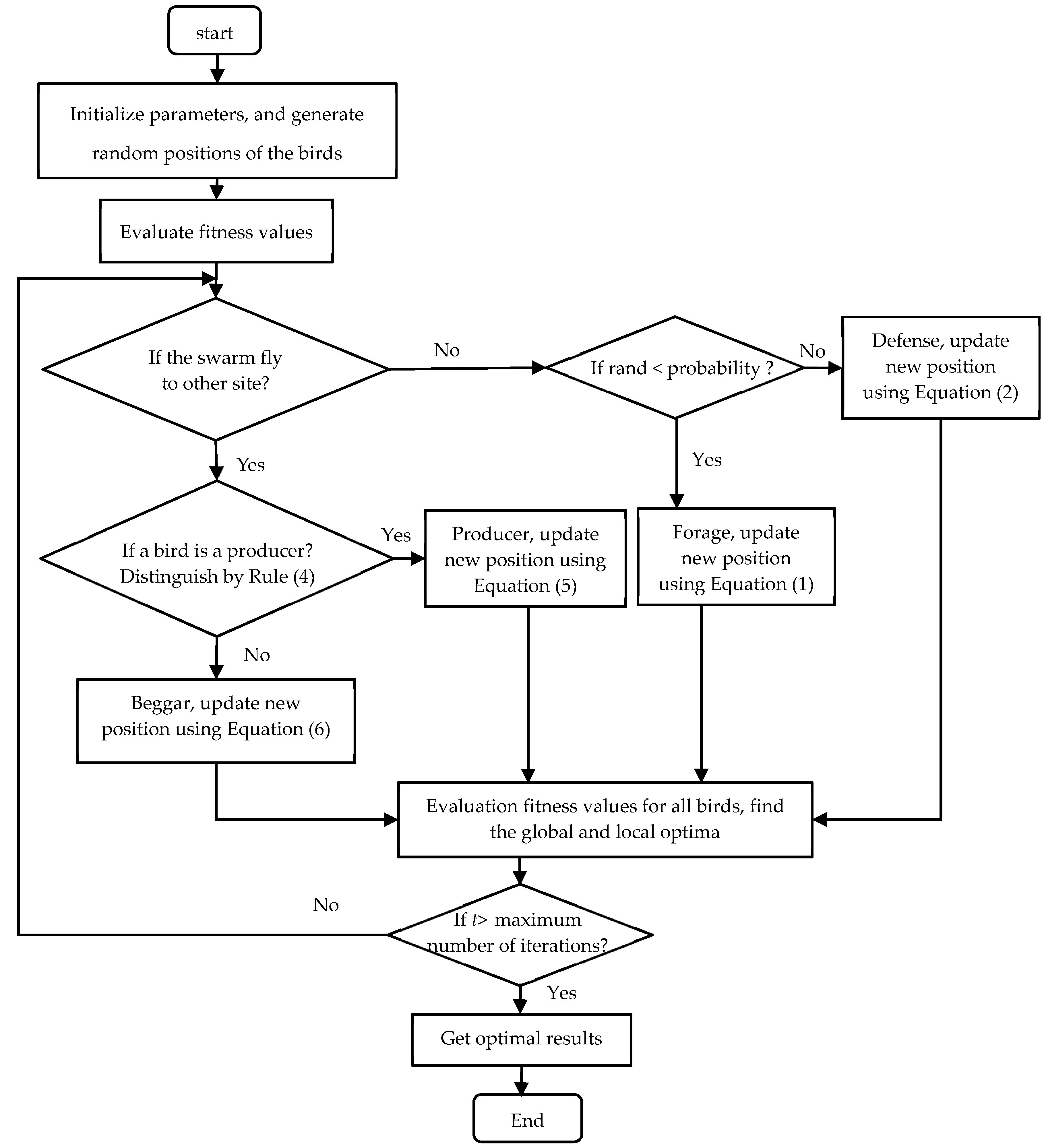
2.3. BSAII
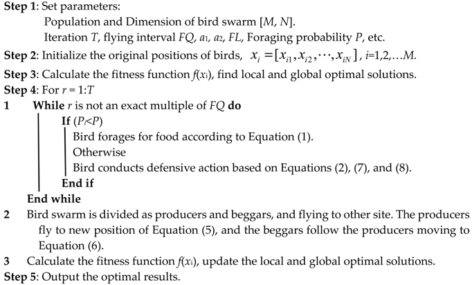
| Algorithm 1. BSAII. |
 |
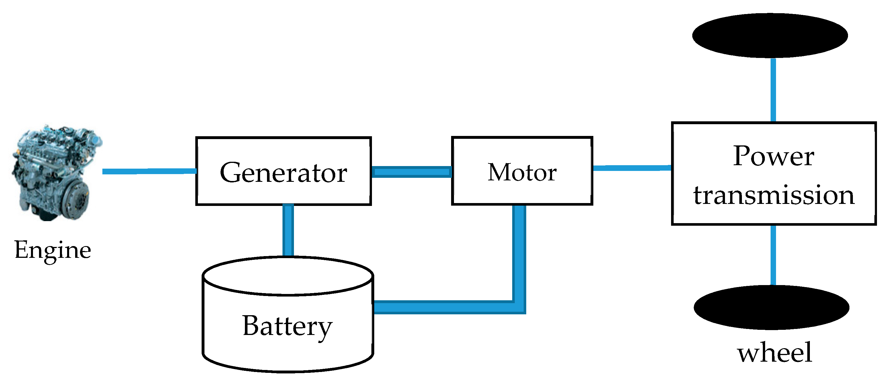
3. Energy Management of E-REV
3.1. Constrained Optimization Problem
3.2. Problem Formulation
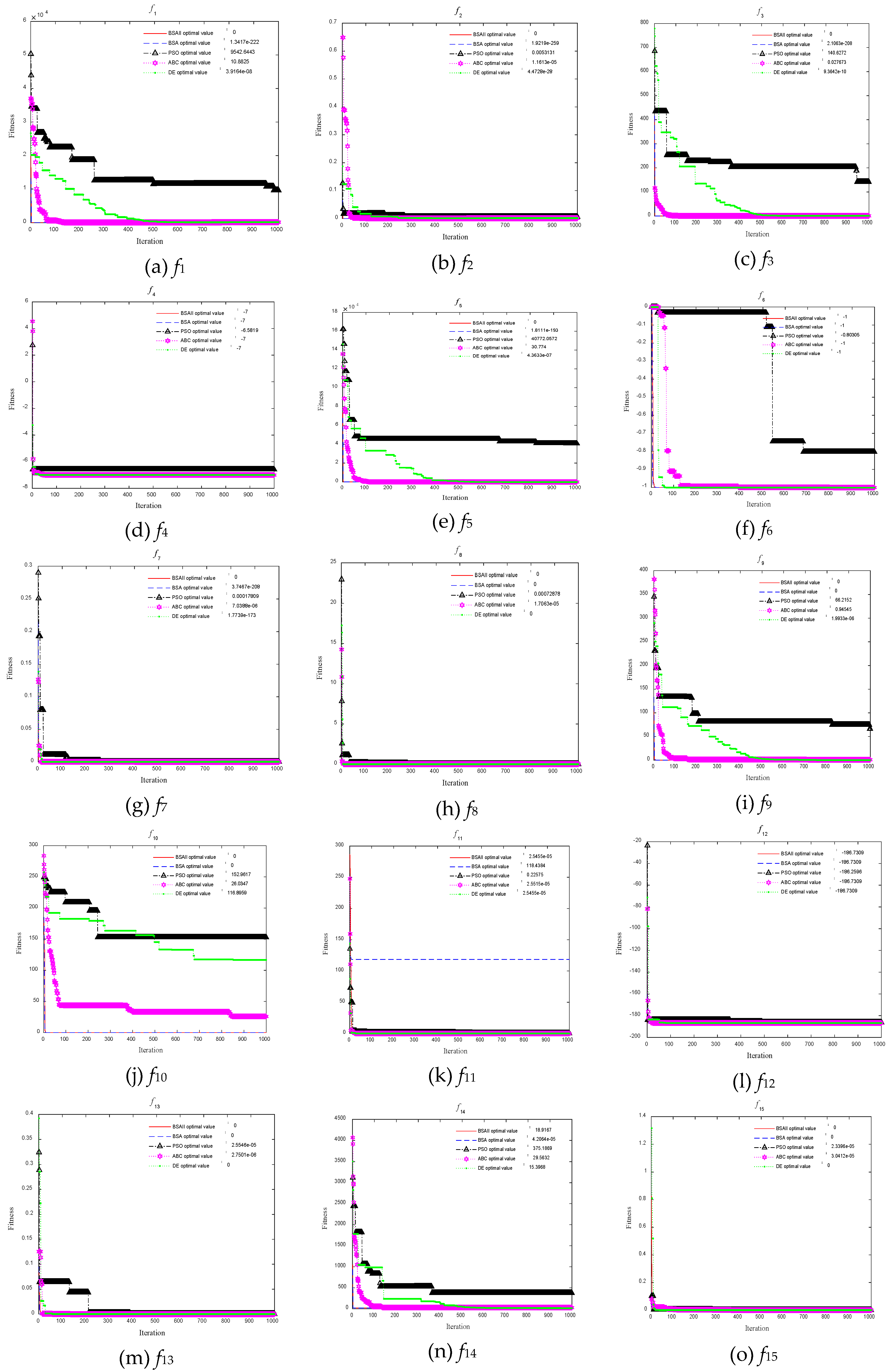
4. Computational Experiment
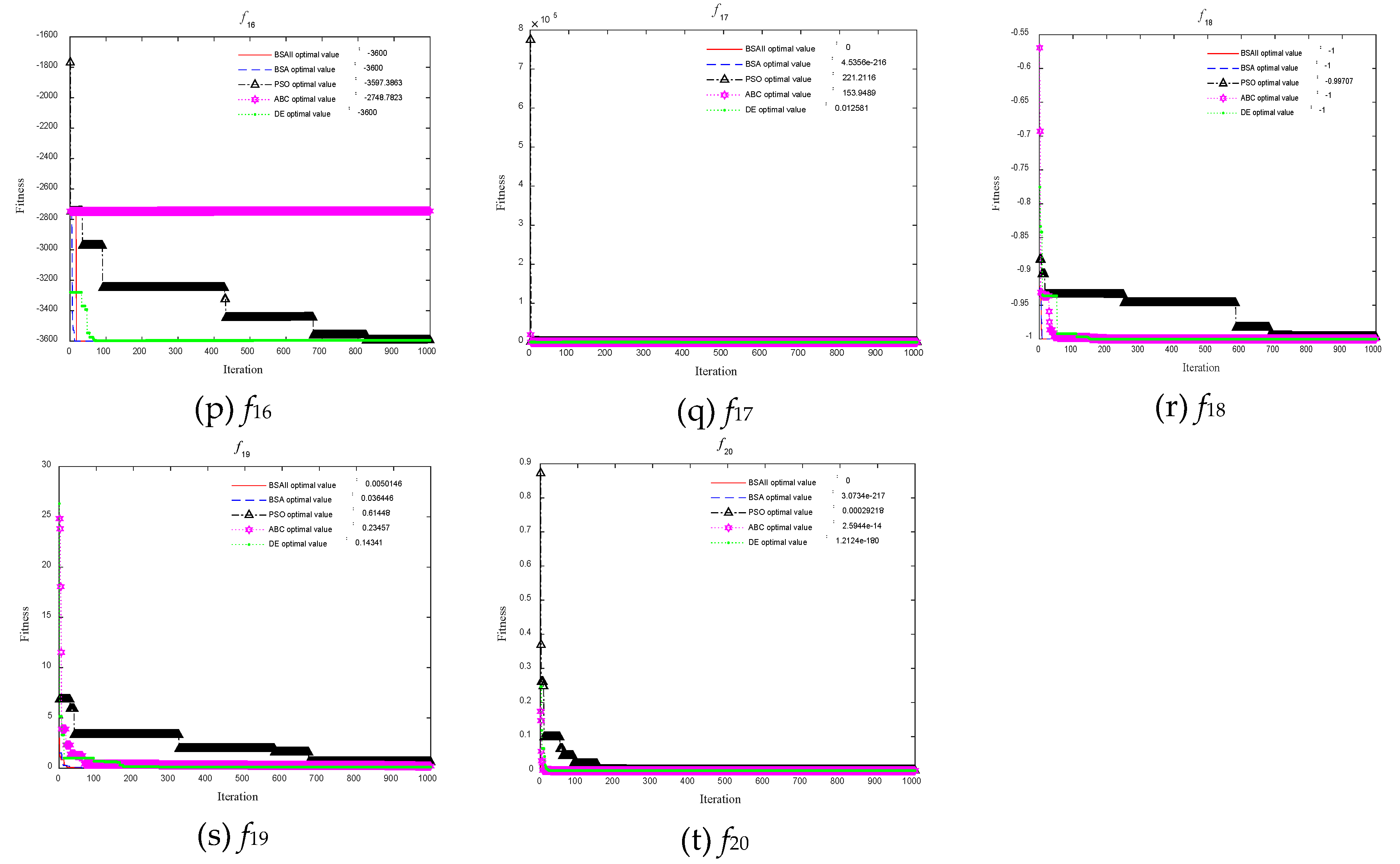
- On instances of f1~f7, f12, f17, and f20, BSAII performed better than other algorithms, in terms of convergence rate and accuracy of optimal solution. Since the four indexes had the smallest values compared with these obtained by other algorithms.
- On instances of f8, it was evident that both BSAII and DE could get the real optima (0 in Table 3), better than the other algorithms.
- On instances of f9 and f10, BSAII and BSA were better than PSO, ABC, and DE in terms of performance indexes.
- On instances of f13, f15 and f18, BSAII, BSA and DE converged to the real optimal value, with the same accuracy. But the convergence rate of BSAII and BSA in the early stage was faster than DE.
- Only on instance of f11, DE acquired the best performance over other algorithms. Solutions found by BSAII and BSA occasionally fell into local optimum.
- Only on instance of f16, BSA converged to the real optimal value (–3600) every time. It was obvious that BSA was better than the other algorithm on this example. While BSAII fell into local optimum at times and was not convergent to –3600. But the average value of 50 trials was closer to the optimum than that obtained by other algorithms.
- The statistical results of f14 and f19 were somewhat complicated. The minimum of optimal fitness on f19 was found by BSAII, but the other three performance indexes of MAX, MEAN, and SD were slightly worse than in DE. BSAII would fall into local optimum when solving benchmark function of f14.
5. Optimization of On-Off Control Mode
5.1. Traditional On-Off Control Mode
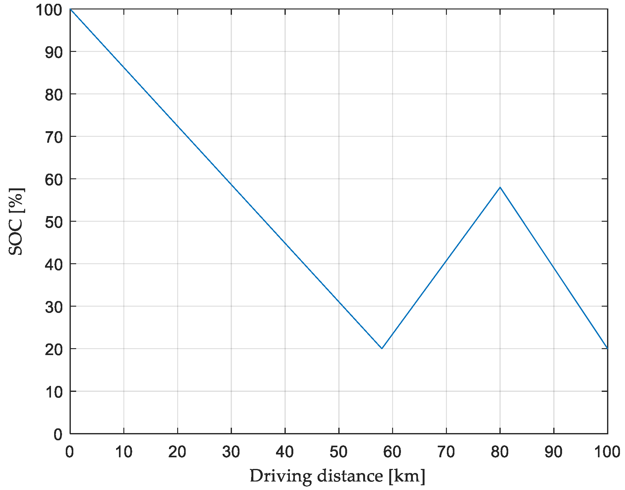
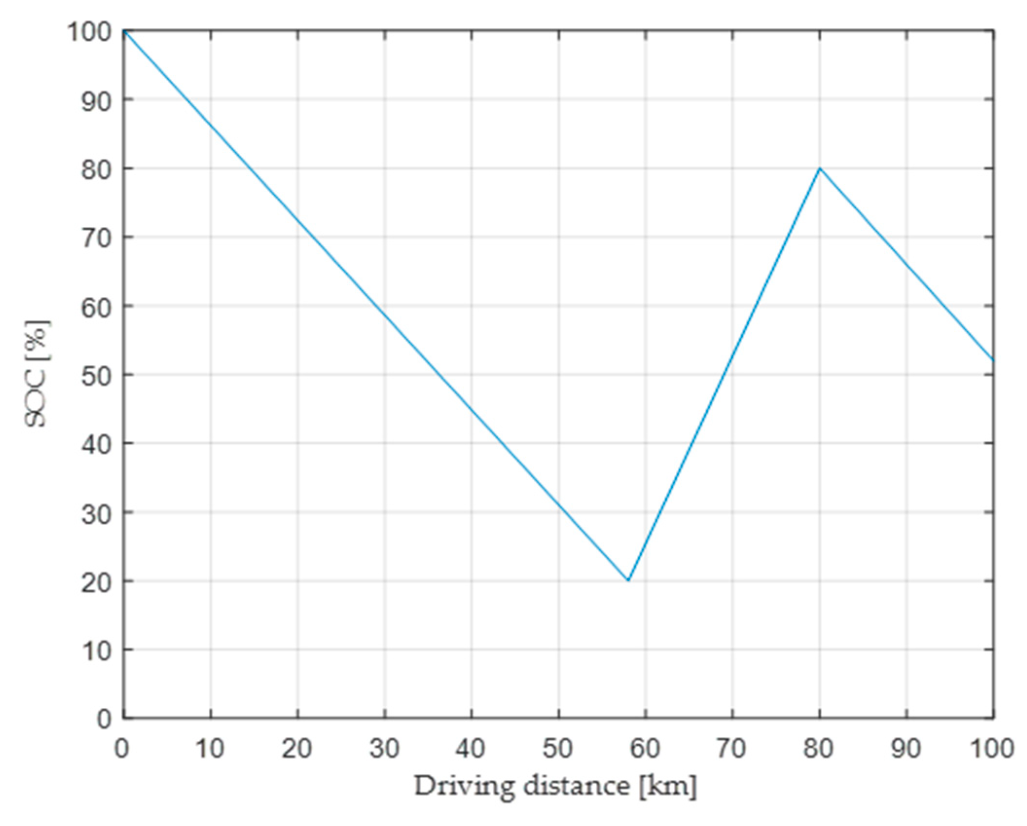
5.1.1. Distance = 100 km
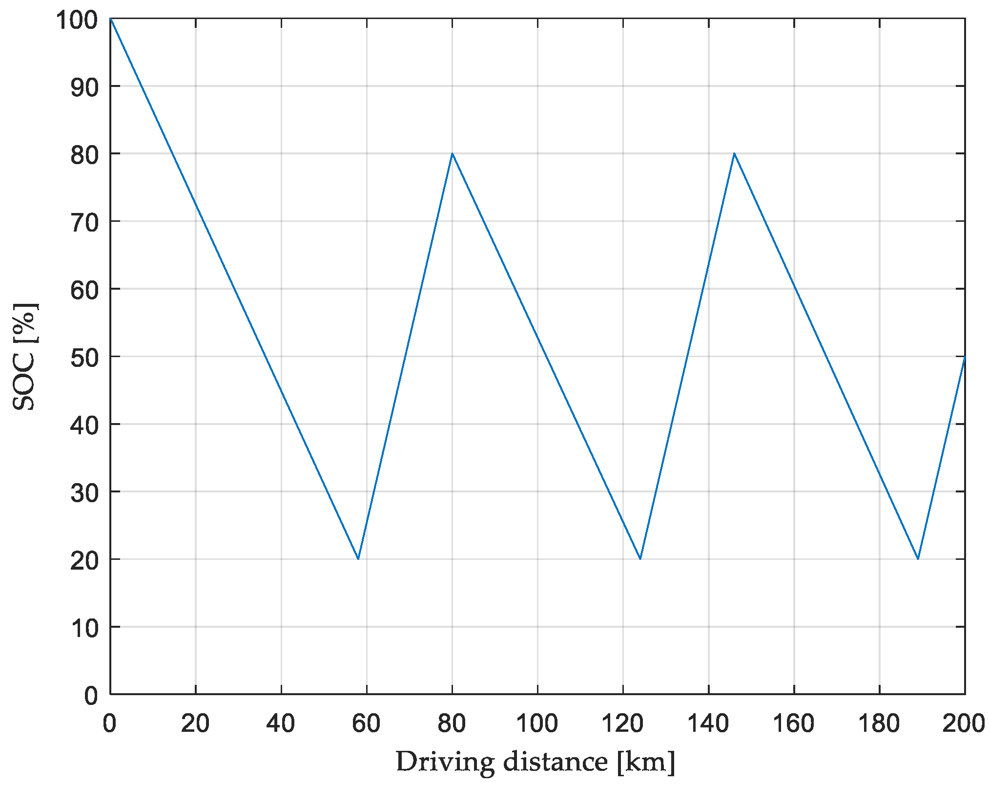
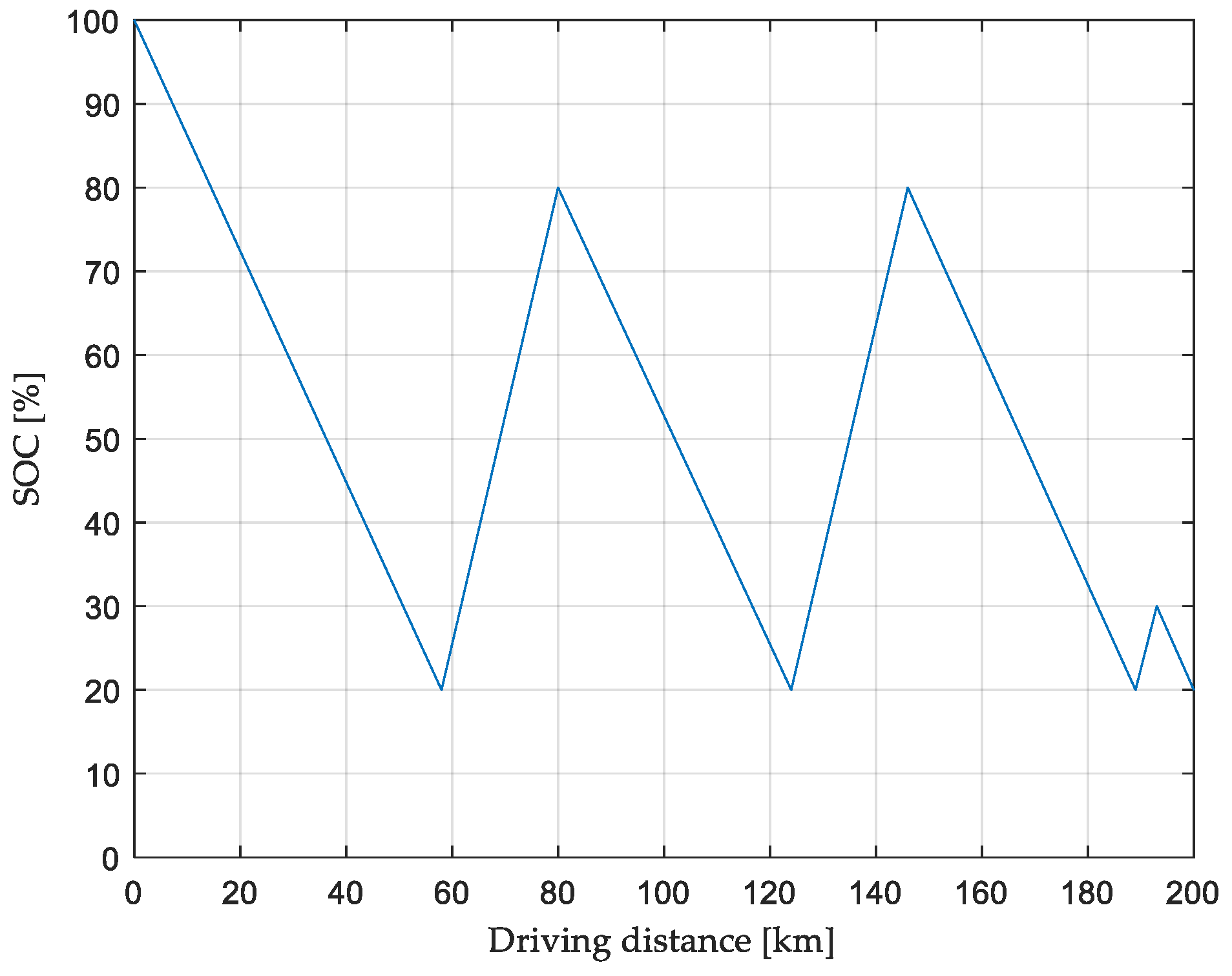
5.1.2. Distance = 200 km
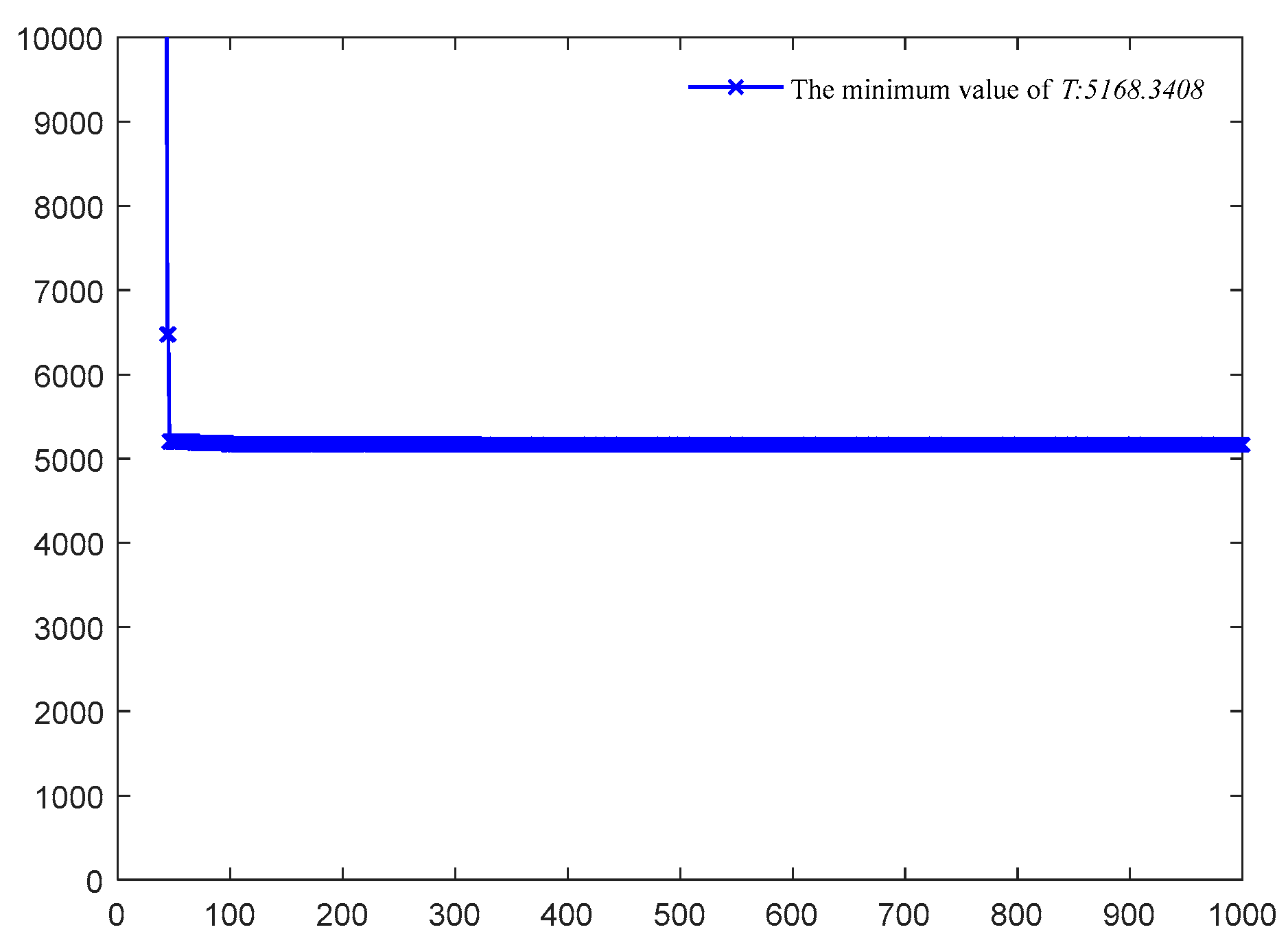
5.2. On-Off Control Mode After Optimization
5.2.1. Distance = 100 km
5.2.2. Distance = 200 km
6. Conclusions
- The BSAII performed statistically superior to or equal to the BSA on 16 benchmark problems. On these problems, it obtained the real optimal solution. However, in the case of Rosenbrock function (f14), it was prone to falling into local optimum.
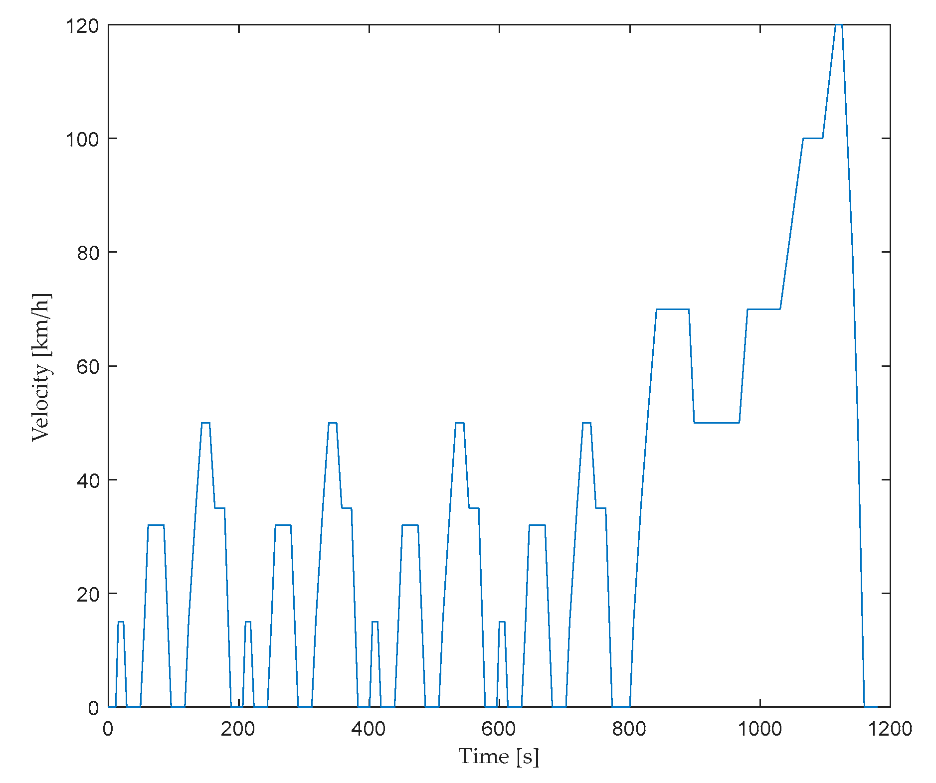
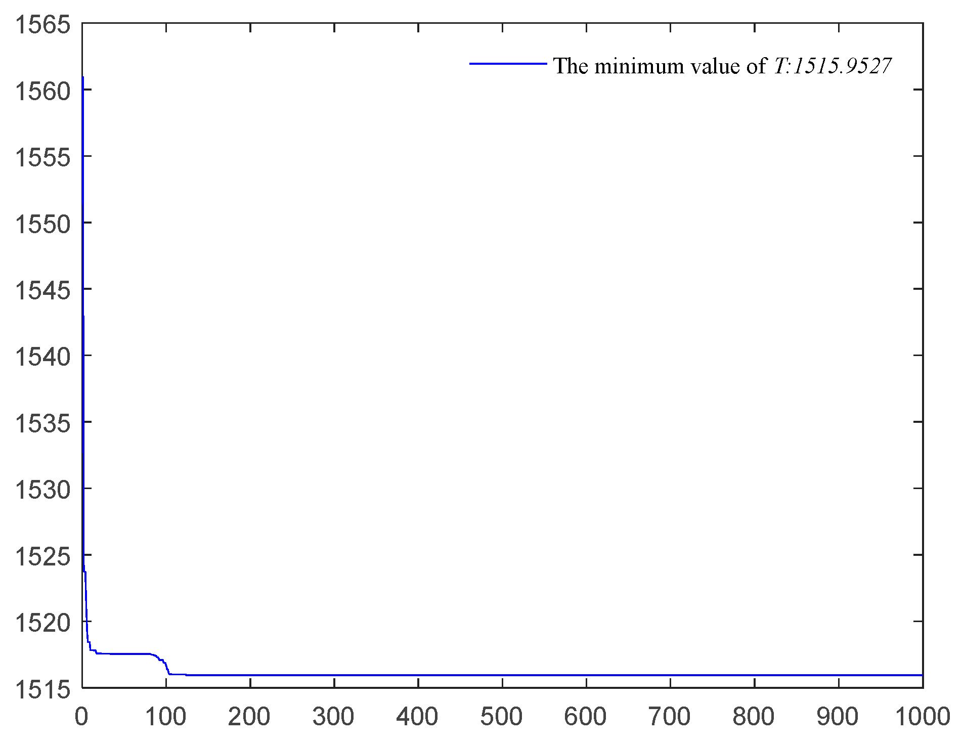
- The energy management of electric vehicles in this paper referred to minimization uptime of RE. The uptime was determined by the time interval between engine on and off. Two instances with different target driving distances were optimized with BSAII. Results indicated that the uptime of engine could be reduced by 36.4% with a target distance of 100 km, and 13% with a target distance of 200 km, respectively, in the NEDC condition. Hence we can draw a conclusion that based on the optimization strategy of BSAII, the on/off timing of the engine can be accurately controlled, which can effectively shorten the uptime of the engine, reduce fuel consumption and exhaust emissions, and also facilitate the next external charging.
Author Contributions
Funding
Conflicts of Interest
References
- Amp, N.J.; Su, Z. On/off timing optimization for the range-extender in extended-range electric vehicles. Automot. Eng. 2013, 35, 418–423. [Google Scholar]
- Zhao, J.; Han, B.; Bei, S. Start-stop moment optimization of range extender and control strategy design for extended-range electric vehicle. In Proceedings of the 5th Asia Conference on Materials Science and Engineering, Tokyo, Japan, 9–11 June 2017. [Google Scholar] [CrossRef]
- Jiang, Y.C.; Zhou, H.; Cheng, L.; Wang, L. A study on energy management control strategy for an extended-range electric vehicle. In Proceedings of the 2015 International Conference on Energy and Mechanical Engineering, Wuhan, China, 17–18 October 2015; pp. 159–169. [Google Scholar]
- Pan, C.F.; Han, F.Q.; Chen, L.; Xu, X.; Chen, L. Power distribution strategy of extend range electric vehicle based on fuzzy control. J. ChongQing Jiaotong Univ. Nat. Sci. 2017, 33, 140–144. [Google Scholar]
- Niu, J.G.; Pei, F.L.; Zhou, S.; Zhang, T. Multi-objective optimization study of energy management strategy for extended-range electric vehicle. Adv. Mater. Res. 2013, 694–697, 2704–2709. [Google Scholar] [CrossRef]
- Abdelgadir, A.A.; Alsawalhi, J.Y. Energy management optimization for an extended range electric vehicle. In Proceedings of the IEEE International Conference on Modeling, Sharjah, UAE, 4–6 April 2017. [Google Scholar]
- Xi, L.H.; Zhang, X.; Geng, C.; Xue, Q.C. Energy management strategy optimization of extended-range electric vehicle based on dynamic programming. J. Traffic Transp. Eng. 2018, 18, 148–156. [Google Scholar]
- Vatanparvar, K.; Faezi, S.; Burago, L.; Levorato, M.; Faruque, M.A.A. Extended range electric vehicle with driving behavior estimation in energy management. IEEE Trans. Smart Grid 2019, 10, 2959–2968. [Google Scholar] [CrossRef]
- Rao, R.V.; Savsani, V.J.; Vakharia, D.P. Teaching-learning-based optimization: A novel method for constrained mechanical design optimization problems. Comput. Aided Des. 2001, 43, 303–315. [Google Scholar] [CrossRef]
- García-Monzó, A.; Migallón, H.; Jimeno-Morenilla, A.; Sanchez-Romero, J.L.; Rico, H.; Rao, R.V. Efficient Subpopulation Based Parallel TLBO Optimization Algorithms. Electronics 2018, 8, 19. [Google Scholar] [CrossRef]
- Mirjalili, S.; Mirjalili, S.M.; Lewis, A. Grey wolf optimizer. Adv. Eng. Softw. 2014, 69, 46–61. [Google Scholar] [CrossRef]
- Al-Moalmi, A.; Luo, J.; Salah, A.; Li, K. Optimal virtual machine placement based on grey wolf optimization. Electronics 2019, 8, 283. [Google Scholar] [CrossRef]
- Fatima, A.; Javaid, N.; Anjum Butt, A.; Sultana, T.; Hussain, W.; Bilal, M.; ur Rehman Hashmi, M.A.; Akbar, M.; Llahi, M. An enhanced multi-objective gray wolf optimization for virtual machine placement in cloud data centers. Electronics 2019, 8, 218. [Google Scholar] [CrossRef]
- Goel, S. Pigeon optimization algorithm: A novel approach for solving optimization problems. In Proceedings of the International Conference on Data Mining & Intelligent Computing, New Delhi, India, 5–6 September 2014. [Google Scholar]
- Duan, H.; Qiao, P.X. Pigeon-inspired optimization: A new swarm intelligence optimizer for air robot path planning. Intern. J. Intell. Comput. Cybern. 2014, 7, 24–37. [Google Scholar] [CrossRef]
- Mirjalili, S.; Lewis, A. The whale optimization algorithm. Adv. Eng. Softw. 2016, 95, 51–67. [Google Scholar] [CrossRef]
- Meng, X.B. A new bio-inspired optimisation algorithm: Bird swarm algorithm. J. Exp. Theor. Artif. Intell. 2015, 28, 673–687. [Google Scholar] [CrossRef]
- Yang, W.R.; Ma, X.Y.; Xu, M.L.; Bian, X.L. Research on scheduling optimization of grid-connected micro-grid based on improved bird swarm algorithm. Adv. Technol. Electr. Eng. Energy 2018, 2, 53–60. [Google Scholar]
- Yang, W.Y.; Ma, X.Y.; Bian, X.L. Optimization of Micro-grid operation using improved bird swarm algorithm under time-of-use price mechanism. Renew. Energy Resour. 2018, 7, 1046–1054. [Google Scholar]
- Yang, W.Y.; Ma, X.Y.; Bian, X.L. Adaptive improved bird swarm algorithm based on levy flight strategy. J. Hebei Univ. Technol. 2017, 5, 10–16, 22. [Google Scholar]
- Zhang, L.; Bao, Q.; Fan, W.; Cui, K.; Xu, H.; Du, Y. An improved particle filter based on bird swarm algorithm. In Proceedings of the 2017 10th International Symposium on Computational Intelligence and Design (ISCID), Hangzhou, China, 9–10 December 2017. [Google Scholar]
- Wang, Y.; Wan, Z.; Peng, Z. A novel improved bird swarm algorithm for solving bound constrained optimization problems. Wuhan Univ. J. Nat. Sci. 2019, 24, 349–359. [Google Scholar] [CrossRef]
- Zahara, E.; Hu, C.H. Solving constrained optimization problems with hybrid particle swarm optimization. Eng. Optim. 2008, 40, 1031–1049. [Google Scholar] [CrossRef]
- Wang, Z.X.; Bei, S.Y.; Wang, W. The optimization control of on and off timing for the engine in extended-range electric vehicle. Mach. Des. Manuf. 2017, 4, 100–103. [Google Scholar]
- Yang, X.S.; Deb, S. Cuckoo search: Recent advances and applications. Neural Comput. Appl. 2014, 24, 169–174. [Google Scholar] [CrossRef]
- Virtual Library of Simulation Experiments: Test Functions and Datasets. Available online: http://www.sfu.ca/~ssurjano (accessed on 30 July 2019).
- Eberhart, R.C.; Shi, Y.H. Particle swarm optimization: Development, application, and resources. In Proceedings of the 2001 Congress on Evolutionary Computation, Seoul, Korea, 27–30 May 2001. [Google Scholar] [CrossRef]
- Storn, R.; Price, K. Differential evolution—A simple and efficient heuristic for global optimization over continuous spaces. J. Glob. Optim. 1997, 11, 341–359. [Google Scholar] [CrossRef]
- Karaboga, D.; Basturk, B. A powerful and efficient algorithm for numerical function optimization: Artificial bee colony (ABC) algorithm. J. Glob. Optim. 2007, 39, 459–471. [Google Scholar] [CrossRef]


| Parameters | Value |
|---|---|
| Curb weight (m/kg) | 1700 |
| Full mass (m/kg) | 2100 |
| Wheel radius (r/m) | 0.334 |
| Windward area (A/m2) | 1.97 |
| Drag coefficients (CD) | 0.32 |
| Maximum speed (km/h) | >140 |
| Total distance (km) | 400 |
| Climbing gradient (%) | >20% |
| Transmission efficiency | 0.95 |
| State of charge (SOC) range (%) | 20–80 |
| Maximum pure electric driving range (km) | >50 |
| Distance of Unit Charge | Driving State | Value [km/%] |
|---|---|---|
| k1 | Initial pure electric | 0.7310 |
| k2 | Charging | 0.3667 |
| k3 | Pure electric after charging | 0.7210 |
| Id. | Name | Dimension | Boundary | Optima |
|---|---|---|---|---|
| f1 | Sphere | 20 | [−100,100] | 0 |
| f2 | Sum of Different Powers | 20 | [−1,1] | 0 |
| f3 | Sum Squares | 20 | [−5.12,5.12] | 0 |
| f4 | Trid | 2 | [−4,4] | –2 |
| f5 | Rotated Hyper-Ellipsoid | 20 | [−65.536,65.536] | 0 |
| f6 | Easom | 2 | [−100,100] | –1 |
| f7 | Matyas | 2 | [−10,10] | 0 |
| f8 | Booth | 2 | [−10,10] | 0 |
| f9 | Griewank | 20 | [−600,600] | |
| f10 | Rastrigin | 20 | [−5.12,5.12] | 0 |
| f11 | Schwefel | 2 | [−500,500] | 0 |
| f12 | Shubert | 2 | [−5.12,5.12] | −186.7309 |
| f13 | Schaffer Function No. 2 | 2 | [−100,100] | 0 |
| f14 | Rosenbrock | 20 | [−2.048,2.048] | 0 |
| f15 | Beale | 2 | [−4.5,4.5] | 0 |
| f16 | Needle in a Haystack | 2 | [−5.12,5.12] | –3600 |
| f17 | Zakharov | 20 | [−5,10] | 0 |
| f18 | Drop-Wave | 2 | [−5.12,5.12] | –1 |
| f19 | Bukin Function No. 6 | 2 | x1∈ [−15,5], x2∈ [−3,3] | 0 |
| f20 | Three-Hump Camel | 2 | [−5,5] | 0 |
| Id. | Function |
|---|---|
| f1 | |
| f2 | |
| f3 | |
| f4 | |
| f5 | |
| f6 | |
| f7 | |
| f8 | |
| f9 | |
| f10 | |
| f11 | |
| f12 | |
| f13 | |
| f14 | |
| f15 | |
| f16 | |
| f17 | |
| f18 | |
| f19 | |
| f20 |
| Algorithm | Parameters |
|---|---|
| BSAII, BSA | |
| PSO | |
| DE | CR = 0.9, F = 0.5 |
| ABC |
| Id. | Algorithm | MIN | MAX | MEAN | SD |
|---|---|---|---|---|---|
| f1 | BSAII | 0 | 0 | 0 | 0 |
| BSA | 6.15 × 10−266 | 9.98 × 10−176 | 2.40 × 10−177 | 0 | |
| PSO | 3150.775 | 11924.62 | 7944.131 | 1938.963 | |
| ABC | 0.1627 | 12.08388 | 3.873986 | 2.878341 | |
| DE | 5.88 × 10−09 | 8.31 × 10−07 | 9.04 × 10−08 | 1.23 × 10−07 | |
| f2 | BSAII | 0 | 0 | 0 | 0 |
| BSA | 5.43 × 10−256 | 2.53 × 10−63 | 5.07 × 10−65 | 3.55 × 10−64 | |
| PSO | 0.000443 | 0.032429 | 0.006521 | 0.00539 | |
| ABC | 1.35 × 10−08 | 1.64 × 10−05 | 2.37 × 10−06 | 3.26 × 10−06 | |
| DE | 2.17 × 10⁻³² | 1.02 × 10⁻²⁰ | 2.05 × 10⁻²² | 1.43 × 10⁻²¹ | |
| f3 | BSAII | 0 | 0 | 0 | 0 |
| BSA | 1.13 × 10−242 | 1.06 × 10−184 | 3.27 × 10−186 | 0 | |
| PSO | 69.29799 | 315.1082 | 196.9478 | 56.54325 | |
| ABC | 0.001651 | 0.036862 | 0.016376 | 0.008962 | |
| DE | 2.98 × 10⁻¹⁰ | 6.99 × 10−09 | 1.51 × 10−09 | 1.27 × 10−09 | |
| f4 | BSAII | −7 | −7 | −7 | 2.66 ×10⁻¹⁵ |
| BSA | −7 | −7 | −7 | 2.29 × 10⁻¹⁴ | |
| PSO | −6.99272 | −6.45886 | −6.90539 | 0.104025 | |
| ABC | −7 | −6.99997 | −6.99999 | 6.26 × 10−06 | |
| DE | −7 | −7 | −7 | 2.66 × 10⁻¹⁵ | |
| f5 | BSAII | 0 | 0 | 0 | 0 |
| BSA | 1.32 × 10−237 | 1.62 × 10−177 | 3.27 × 10−179 | 0 | |
| PSO | 8375.27 | 48805.58 | 30703.65 | 7607.746 | |
| ABC | 1.394579 | 48.57402 | 14.07298 | 9.398897 | |
| DE | 2.91 × 10−08 | 5.71 × 10−07 | 1.59 × 10−07 | 1.12 × 10−07 | |
| f6 | BSAII | −1 | −1 | −1 | 0 |
| BSA | −1 | −1 | −1 | 3.94 × 10⁻¹⁴ | |
| PSO | −0.99599 | −1.18 × 10−69 | −0.29917 | 0.334968 | |
| ABC | −1 | −8.11 × 10−05 | −0.9555 | 0.197304 | |
| DE | −1 | −1 | −1 | 0 | |
| f7 | BSAII | 0 | 0 | 0 | 0 |
| BSA | 3.79 × 10−251 | 2.53 × 10−179 | 5.07 × 10−181 | 0 | |
| PSO | 1.75 × 10−05 | 0.002047 | 0.000348 | 0.000447 | |
| ABC | 2.20 × 10−07 | 0.000157 | 3.22 × 10−05 | 3.99 × 10−05 | |
| DE | 1.42 × 10−178 | 2.10 × 10−170 | 6.36 × 10−172 | 0 | |
| f8 | BSAII | 0 | 0 | 0 | 0 |
| BSA | 0 | 1.36 × 10⁻¹⁴ | 2.72 × 10⁻¹⁶ | 1.90 × 10⁻¹⁵ | |
| PSO | 0.000117 | 0.054104 | 0.011096 | 0.012605 | |
| ABC | 2.91 × 10−08 | 0.000174 | 3.09 × 10−05 | 3.93 × 10−05 | |
| DE | 0 | 0 | 0 | 0 | |
| f9 | BSAII | 0 | 0 | 0 | 0 |
| BSA | 0 | 0 | 0 | 0 | |
| PSO | 36.51811 | 113.051 | 77.5095 | 17.99438 | |
| ABC | 0.669883 | 1.17361 | 1.027435 | 0.086522 | |
| DE | 5.34 × 10−08 | 0.027025 | 0.003197 | 0.006494 | |
| f10 | BSAII | 0 | 0 | 0 | 0 |
| BSA | 0 | 0 | 0 | 0 | |
| PSO | 118.5101 | 174.2391 | 150.3891 | 13.19794 | |
| ABC | 16.57457 | 41.5169 | 28.29116 | 5.126784 | |
| DE | 83.19845 | 134.5668 | 110.4572 | 12.10043 | |
| f11 | BSAII | 2.55 × 10−05 | 118.4384 | 40.26906 | 56.10528 |
| BSA | 2.55 × 10−05 | 118.4384 | 30.79399 | 51.95111 | |
| PSO | 0.004037 | 21.11573 | 2.520817 | 4.011557 | |
| ABC | 2.55 × 10−05 | 6.29 × 10−05 | 2.97 × 10−05 | 6.14 × 10−06 | |
| DE | 2.55 × 10−05 | 2.55 × 10−05 | 2.55 × 10−05 | 0 | |
| f12 | BSAII | −186.731 | −186.731 | −186.731 | 9.59 ×10⁻¹⁴ |
| BSA | −186.731 | −186.731 | −186.731 | 9.80 × 10−07 | |
| PSO | −186.717 | −184.601 | −186.243 | 0.436279 | |
| ABC | −186.731 | −186.731 | −186.731 | 3.28 × 10−06 | |
| DE | −186.731 | −186.731 | −186.731 | 9.99 × 10⁻¹⁴ | |
| f13 | BSAII | 0 | 0 | 0 | 0 |
| BSA | 0 | 0 | 0 | 0 | |
| PSO | 2.70 × 10−06 | 0.017705 | 0.005071 | 0.004228 | |
| ABC | 8.24 × 10⁻¹⁰ | 1.85 × 10−05 | 2.82 × 10−06 | 3.96 × 10−06 | |
| DE | 0 | 0 | 0 | 0 | |
| f14 | BSAII | 18.83609 | 18.97269 | 18.90242 | 0.029108 |
| BSA | 9.70 ×10⁻¹³ | 18.80166 | 1.304165 | 4.264392 | |
| PSO | 151.1679 | 709.0956 | 455.849 | 117.039 | |
| ABC | 19.55623 | 51.37853 | 28.38958 | 7.592035 | |
| DE | 12.17635 | 16.29873 | 14.56445 | 0.859034 | |
| f15 | BSAII | 0 | 0 | 0 | 0 |
| BSA | 0 | 0 | 0 | 0 | |
| PSO | 2.86 × 10−05 | 0.012789 | 0.001782 | 0.002403 | |
| ABC | 2.63 × 10−08 | 0.000207 | 5.00 × 10−05 | 5.51 × 10−05 | |
| DE | 0 | 0 | 0 | 0 | |
| f16 | BSAII | −3600 | −2748.78 | -3565.95 | 166.8039 |
| BSA | −3600 | −3600 | −3600 | 0 | |
| PSO | −3599.74 | −3024.95 | −3504.13 | 103.0209 | |
| ABC | −3598.49 | −2748.78 | −3307.88 | 297.6948 | |
| DE | −3600 | −2748.78 | −2919.03 | 340.4871 | |
| f17 | BSAII | 0 | 0 | 0 | 0 |
| BSA | 1.21 × 10−240 | 3.65 × 10−54 | 7.34 × 10−56 | 5.11 × 10−55 | |
| PSO | 60.66649 | 438.8272 | 203.5698 | 81.22512 | |
| ABC | 101.2244 | 178.586 | 140.5003 | 16.80537 | |
| DE | 0.003087 | 0.190539 | 0.042672 | 0.037769 | |
| f18 | BSAII | −1 | −1 | −1 | 0 |
| BSA | −1 | −1 | −1 | 0 | |
| PSO | −0.99988 | −0.93622 | −0.97521 | 0.020419 | |
| ABC | −1 | −0.99996 | −0.99999 | 7.72 × 10−06 | |
| DE | −1 | −1 | −1 | 0 | |
| f19 | BSAII | 7.97 ×10−05 | 0.14995 | 0.066484 | 0.041502 |
| BSA | 0.002607 | 0.147479 | 0.070706 | 0.039185 | |
| PSO | 0.169037 | 1.416421 | 0.729224 | 0.272299 | |
| ABC | 0.041325 | 0.298631 | 0.166209 | 0.043545 | |
| DE | 0.00036 | 0.126775 | 0.063711 | 0.038273 | |
| f20 | BSAII | 0 | 0 | 0 | 0 |
| BSA | 8.88 × 10−249 | 6.76 × 10−170 | 1.35 × 10−171 | 0 | |
| PSO | 1.16×10−05 | 0.003825 | 0.000797 | 0.000874 | |
| ABC | 1.00 × 10⁻¹⁶ | 3.08 × 10⁻¹¹ | 1.96 × 10⁻¹² | 5.64 × 10⁻¹² | |
| DE | 2.31 × 10−187 | 1.66 × 10−178 | 3.68 × 10−180 | 0 |
| Mode | Time [%] | Distance [km] | Working time [s] |
|---|---|---|---|
| ton | 20 | 58 | 2383 s |
| toff | 80 | 80 |
| Mode | Time [%] | Distance [km] | Working time [s] |
|---|---|---|---|
| ton | 20 | 189 | 5959 s |
| toff | 50 | 200 |
| Mode | Time [%] | Distance [km] | Working time [s] |
|---|---|---|---|
| ton | 20 | 58 | 1515 s |
| toff | 58 | 80 |
| Mode | Time [%] | Distance [km] | Working time [s] |
|---|---|---|---|
| ton | 20 | 189 | 5168 s |
| toff | 30 | 193 |
© 2019 by the authors. Licensee MDPI, Basel, Switzerland. This article is an open access article distributed under the terms and conditions of the Creative Commons Attribution (CC BY) license (http://creativecommons.org/licenses/by/4.0/).
Share and Cite
Wu, D.; Feng, L. On-Off Control of Range Extender in Extended-Range Electric Vehicle using Bird Swarm Intelligence. Electronics 2019, 8, 1223. https://doi.org/10.3390/electronics8111223
Wu D, Feng L. On-Off Control of Range Extender in Extended-Range Electric Vehicle using Bird Swarm Intelligence. Electronics. 2019; 8(11):1223. https://doi.org/10.3390/electronics8111223
Chicago/Turabian StyleWu, Dongmei, and Liang Feng. 2019. "On-Off Control of Range Extender in Extended-Range Electric Vehicle using Bird Swarm Intelligence" Electronics 8, no. 11: 1223. https://doi.org/10.3390/electronics8111223
APA StyleWu, D., & Feng, L. (2019). On-Off Control of Range Extender in Extended-Range Electric Vehicle using Bird Swarm Intelligence. Electronics, 8(11), 1223. https://doi.org/10.3390/electronics8111223