1. Introduction
Non-thermal atmospheric pressure plasmas are intensively investigated and used in a wide range of research fields and industrial domains such as in aeronautics and aerospace, surface treatment processes, air and water pollutant abatement and biomedical applications [
1,
2,
3,
4,
5,
6,
7]. Dielectric barrier discharges (DBDs) are often used as non-thermal plasma sources because they allow the generation of a homogeneously distributed non-thermal plasma at atmospheric pressure in a cheap way. Furthermore, they are easy to build in a multitude of geometries and can be easily scaled up [
1]. A DBD reactor is made by two electrodes separated by one or more dielectric layers [
8]. Several reactor geometries have been investigated in the last decades [
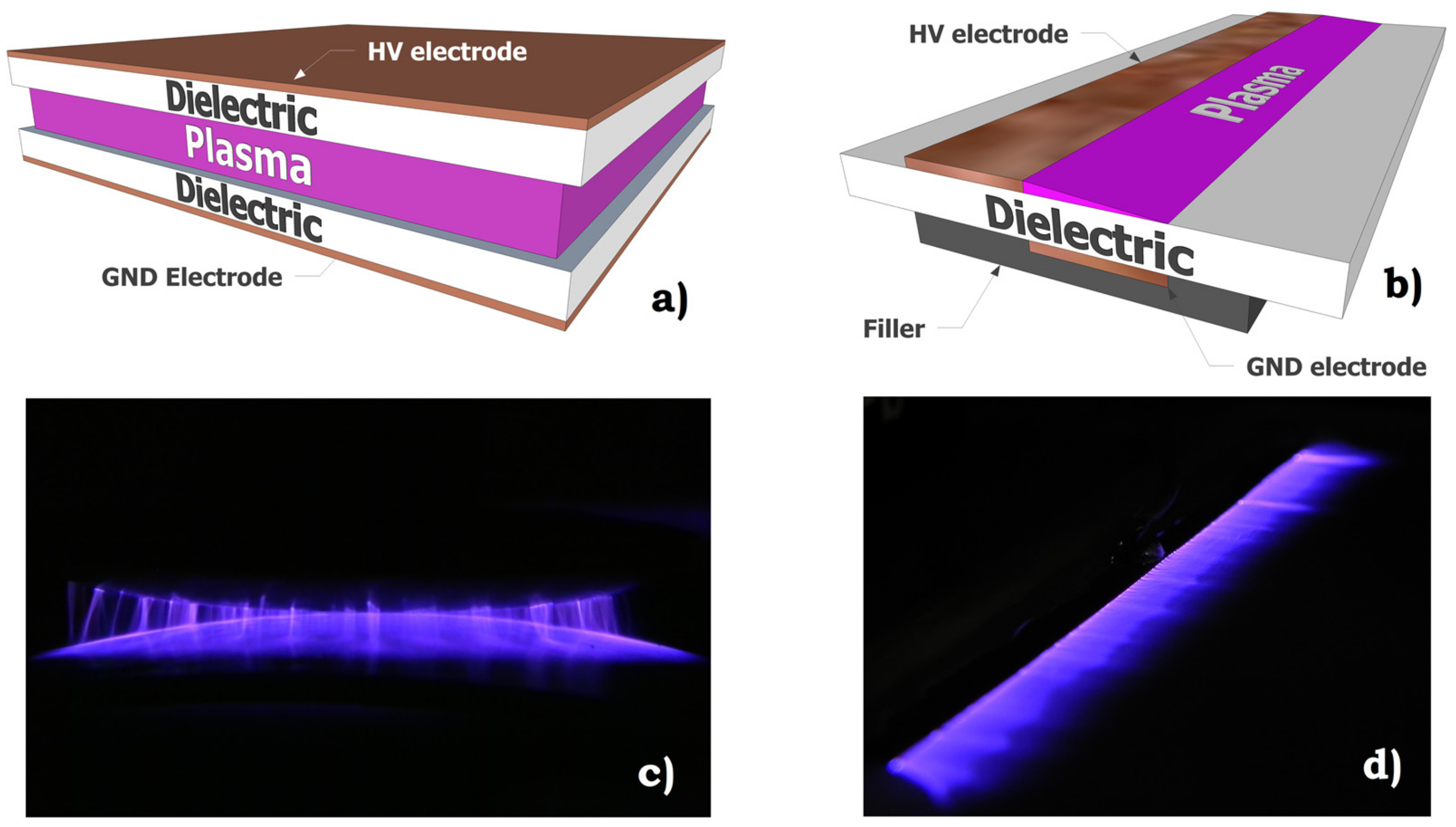
9]. In this work, two of the most commonly used reactor geometries have been employed to test the generator: the volumetric discharge with hemispherical plates and the surface discharge. Reactor sketches and corresponding generated discharges are displayed in
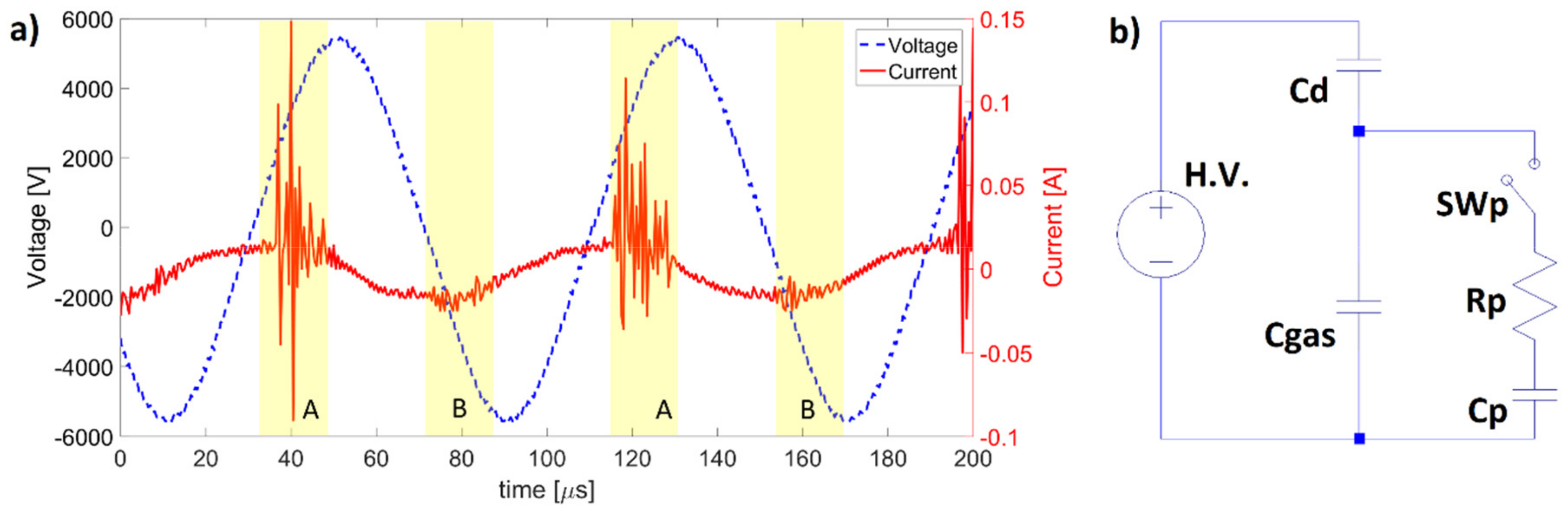
Figure 1. When a variable voltage, with high enough amplitude, is applied to the electrodes, the gas breakdown occurs. The representative voltage–current characteristic of a sinusoidal supplied DBB load is presented in
Figure 2a.
Plasma is macroscopically ignited twice each voltage period (A and B intervals highlighted in light yellow in the figure [
10]. Within each of these time intervals, the plasma with a streamer nature appears (the red line of the current is no more sinusoidal in these intervals). Streamer (which is a plasma filament) repetition rate is usually in the range from 1 to 10 MHz with lifetimes of few tens of nanoseconds [
1]. A simplified equivalent circuit of a DBD is presented in
Figure 2b where
Cd and
Cgas are equivalent capacities of dielectric and gas gaps, respectively. The switch
SWp is closed every time a plasma streamer is formed (i.e., in the MHz range). The presence of the plasma resistance
Rp reflects average power used by the discharge to ionize the gas, the plasma capacity
Cp takes into account the increase in the overall reactor capacity when the plasma is ignited [
1]. This equivalent circuit is strongly capacitive with power factors typically below 0.05.
In plasma medicine applications, surface modification and chemical activation due to the plasma effect is strongly energy-dose-dependent [
11]. Thus, the knowledge of the average power feeding the discharge is a crucial parameter to be evaluated. Moreover, when a high amount of power is requested (as an example in ozone generation for air or water sanification [
12]), the efficiency of the high-voltage power supply must be considered too. In this way an environmentally friendly process is achieved.
Several power supply typologies used to feed DBD loads have been presented in the last decade. Sinusoidal [
1], pulsed [
11,
12,
13,
14] and arbitrary voltage waveforms [
15,
16] are the most used ones. Due to the low cost and robustness, sinusoidal power sources are frequently preferred. AC power supplies are usually constituted by a low-voltage section and a step-up transformer. The discharge can be ignited directly at the net frequency (50 or 60 Hz) [
17], or at increased frequencies, by using power electronic components. Several architectures with one [
18], two [
19] or four [
20] electronic switches have been utilized. Transformer-less configurations have been used as well [
21].
In this paper a high-voltage power supply based on a push–pull converter, controlled by an Arduino DUE micro-controller and equipped with on-board diagnostic is presented. This voltage source is used to produce DBD non-thermal discharges at atmospheric pressure with a self-tuned working frequency. The self-tuning depends on the load impedance and guarantees a high efficiency and a low wear of the components. Output voltage and average power delivered to the discharge are detected and monitored in a quasi-real-time way without the use of an expensive external measurement setup. This power source allows to supply the load continuously or with on/off modulation cycles. An optimization of these voltage waveform trains is usually crucial in aeronautics [
22,
23] and in treatment processes [
24,
25]. LTspice software [
26] has been utilized to better understand the behavior of the generator and to compare experimental measurements and simulation results.
This paper is divided as follows. Firstly, the power supply architecture is presented in
Section 2. Then, the reasons for using the Arduino 2 micro-controller are given. The average power measurements and basic generator operations are provided in
Section 4 and
Section 5, respectively. The proposed self-tuning control strategy is described in
Section 6. Finally, conclusions are given.
2. Power Supply Architecture
The supply source presented in this work can generate a sinusoidal high-voltage output up to 20 kV peak with a variable frequency in the range between 10 and 60 kHz with an output average power up to 200 W. The generator architecture is based on a commercial low-voltage AC/DC converter feeding a push–pull high-voltage transformer (
Figure 3). The commercial AC/DC converter is rated with voltages up to 40 V (VDC in
Figure 3) and currents up to 10 A. This typology of the DC power source has been chosen because of its robustness, availability on the market, and safety reasons.
The PWM control signal is generated by a TL494 integrated circuit. IRF3415 MOSFETs have been utilized as switches. The micro-controller Arduino DUE is used both to regulate the switching frequency and to sample the two signals
Vout and
VCm. The former is varied by changing the value of a digital potentiometer connected to the oscillator frequency pin of the TL494 integrated circuit. The sampling circuit, the on-board voltage divider and the presence of the measurement capacitor
Cm shown in
Figure 3 will be described later on. Each primary winding is constituted by 7 turns (
N1/2 in the figure), the secondary one by 1000 turns (
N2 in the figure). The high-voltage winding is a commercial one, and it is insulated by means of a silicon rubber potting. The components
Ds,
Rs and
Cs in
Figure 3 constitute snubber circuits utilized to limit MOSFET overvoltages during commutations.
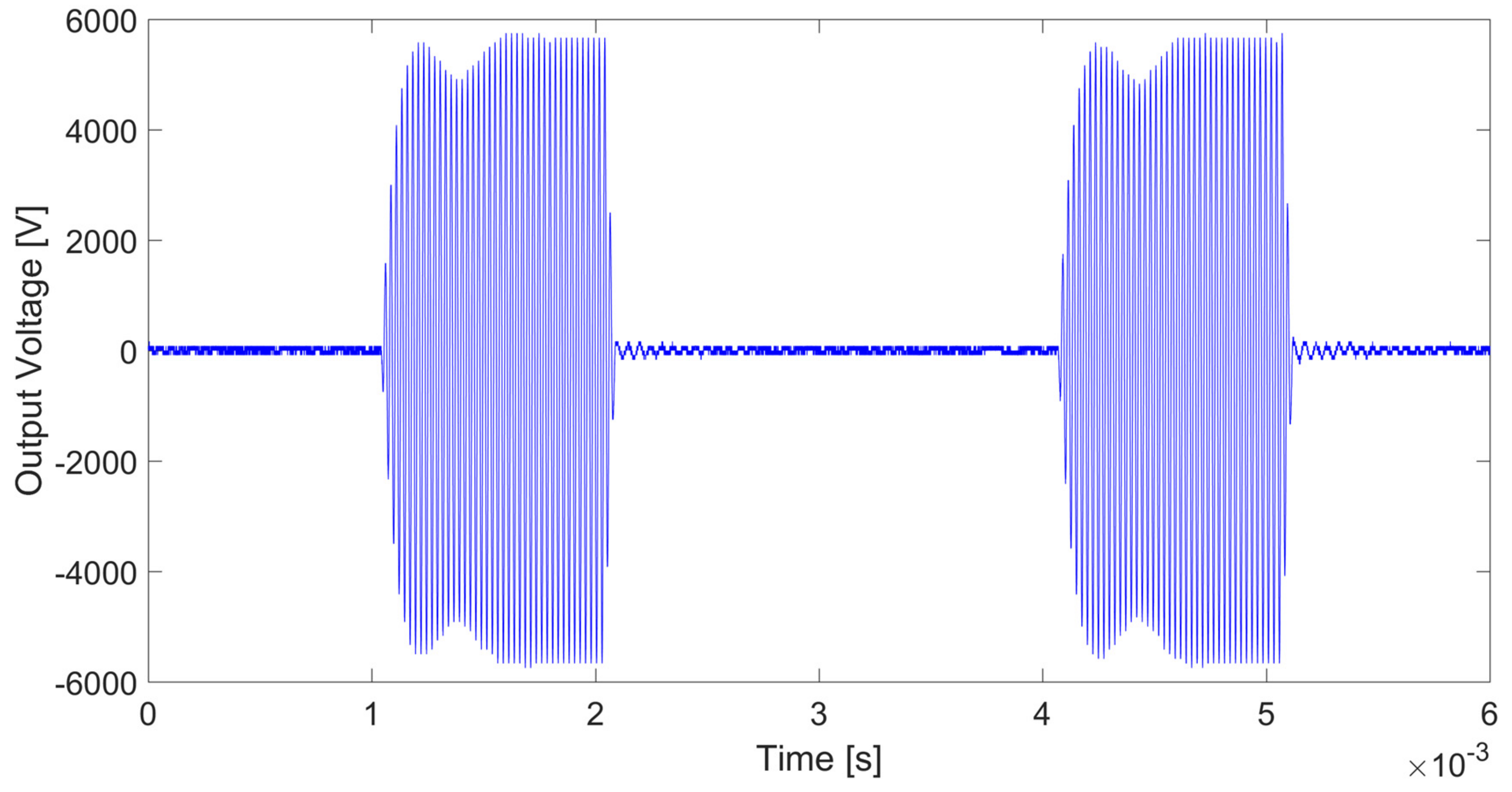
Another important feature of this power supply is the possibility to modulate the output voltage with on/off cycles. An example of on/off voltage modulation with on- and off times equal to 1 and 2 ms respectively, is presented in
Figure 4. The plasma generation frequency has been set to 40 kHz. This means that for each on-time interval, 40 waveform cycles are generated. The figure shows a transient of about 500 μs after the switching-on phase and an almost negligible one after the switching-off phase. As already mentioned, this modulation strategy is a key-role parameter in several research and industrial applications to achieve both effective and efficient treatments.
3. Reasons for Using Arduino DUE Micro-Controller
The main features of this supply system are its flexibility, the possibility to visualize output voltage and average power feeding the discharge, and to self-detect and tune the best working frequency depending on the load connected to it. As will be described in the following, the working frequency allows both to maximize generator efficiency and to decrease MOSFETs’ electrical stress. Arduino DUE has been chosen because it is a low-cost micro-controller, able to detect analog signals with a sample rate frequency up to 500 kHz. As far as the maximum output frequency is 60 kHz, according to the Nyquist-Shannon sampling theorem, a 500 kHz sample rate guarantees a correct sampling of the signal up the fourth harmonic. For lower working frequencies this condition can be fulfilled even for a higher harmonic content.
The high-voltage signal Vout is detected by means of an on-board resistive divider capacitively compensated and sampled by the micro-controller. This voltage divider is constituted by the series of 20 high-voltage resistors, each one rated with 2 MΩ, 3 kV. The measurement resistor, in series with the other 20 high-voltage ones, is connected to the ground terminal and it is rated with 1.5 kΩ, 100 V. Each high-voltage resistor has in parallel a high-voltage capacitor, 220 pF, 3 kV. The measurement resistor has in parallel a 15 pF, 100 V capacitor.
The average power P feeding the discharge is given by:
where T is the waveform period and
vout and
iout are the voltage and current feeding the load, respectively.
The harmonic content of the plasma current feeding a DBD reactor is typically in the range between 1 and 10 MHz (see [
1] and
Figure 2a). Thus, a correct evaluation of the average power feeding the discharge must be done by using both a current probe and an analog/digital converter with an appropriate bandwidth reasonably higher than 10 MHz. In order to contain the costs of the generator, the average power has been evaluated by using the Lissajous charge–voltage figures [
27]. The charge measurement is done by means of the insertion of a shunt capacitance (
Cm in
Figure 3 and
Figure 5a) in series with the load. The capacitance must be several orders of magnitude higher than the reactor capacitance so that its influence on the voltage across the discharge gap is negligible. For this reason, a value of 10 nF has been chosen. The charge
qm accumulated by the
Cm capacitor can be expressed by using the capacitor voltage drop
VCm as
. By considering that the current feeding the load is
, Equation (1) can be expressed as:
The last integral represents the energy delivered to the discharge in one waveform cycle and can be calculated as the area enclosed by the
Vout–Qm curve in the Lissajous diagram. As far as this is an integral method, the requested sample rate is the same used for the applied voltage
Vout. Thus, the micro-controller can be used to evaluate the average power when the Lissajous figure technique is used. In
Figure 5b, an example of Lissajous figure is displayed. Regions “A” and “B” correspond to the time intervals in which the discharge is ignited (see
Figure 2a). As far as the slope of the Lissajous curve is equal to the equivalent capacitance of the load, it is possible to note that the equivalent capacitance of the reactor when the discharge is ignited (“A” and “B” intervals), is about twice the equivalent capacitance without the presence of plasma. This behavior was already introduced when the equivalent discharge circuit was introduced in
Figure 2b.
The creation of the on/off output voltage modulation (see
Figure 4) is controlled by the micro-controller, inhibiting the TL494 PWM generation. The main information of working frequency, maximum output voltage, average power and on- and off-time intervals of the output modulation are available onto an on-board display or directly in a PC monitor.
5. Basic Generator Operations
In DBD plasmas working at several kilovolts and several tens of kHz, the discharge regime is not strictly related with the value of the supplying frequency, because the streamer generation frequency is always in the megahertz range, with the plasma filament life-time of the order of tens of nanoseconds [
1]. Supplying frequency mostly influences the number of periods per second in which plasma occurs. The most important parameter related to discharge effects is usually the average power feeding the discharge. An example is given by the ozone production obtained through a DBD plasma discharge. The ozone yield remains practically the same in the frequency range between 10 and 50 kHz. Working at constant voltage, a frequency increase leads to a higher discharge power and an increment of the ozone generated, keeping constant the energy cost for the ozone production [
10,
12]. In the aeronautics field, the same induced velocity can be obtained by using a DBD plasma actuator fed with the same average power obtained with different voltage-frequency values [
28]. Thus, the working frequency can be selected using criteria related to the best performance of the power source, subsequently adjusting the supplying voltage to obtain the desired average power. In the experiments presented in this work, the chosen frequency maximizes the power supply efficiency through its dependence on the load impedance and minimizes the wear of components.
The possibility to vary the switching frequency is an important feature of this supply source. By changing this parameter, both different commutation regimes of the MOSFETs and different supply voltage harmonic contents are obtained. When the DBD reactor is connected to the high-voltage terminals, the switching frequency can be varied to achieve a soft switching condition. In this regime a zero-current switching (ZCS) is obtained, strongly limiting the overvoltages of the MOSFETs and thus minimizing the power dissipation into the snubber circuits.
To better understand the behavior of the generator as a function of the switching frequency, LTspice software has been utilized. MOSFETs have been implemented by using the Spice model available in the International Rectifier website. The magnetic coupling between windings has been implemented by using the mutual inductance coefficient
K. By following LTspice user manual this parameter can be calculated as:
where
L is the winding self-inductance and
Lleak is the leakage inductance between the windings considered. Self and leakage inductances have been measured for all windings by using an Asita AS250 impedance meter. A substantial symmetry has been found, leading to the definition of a
K value equal to 0.94 for all windings.
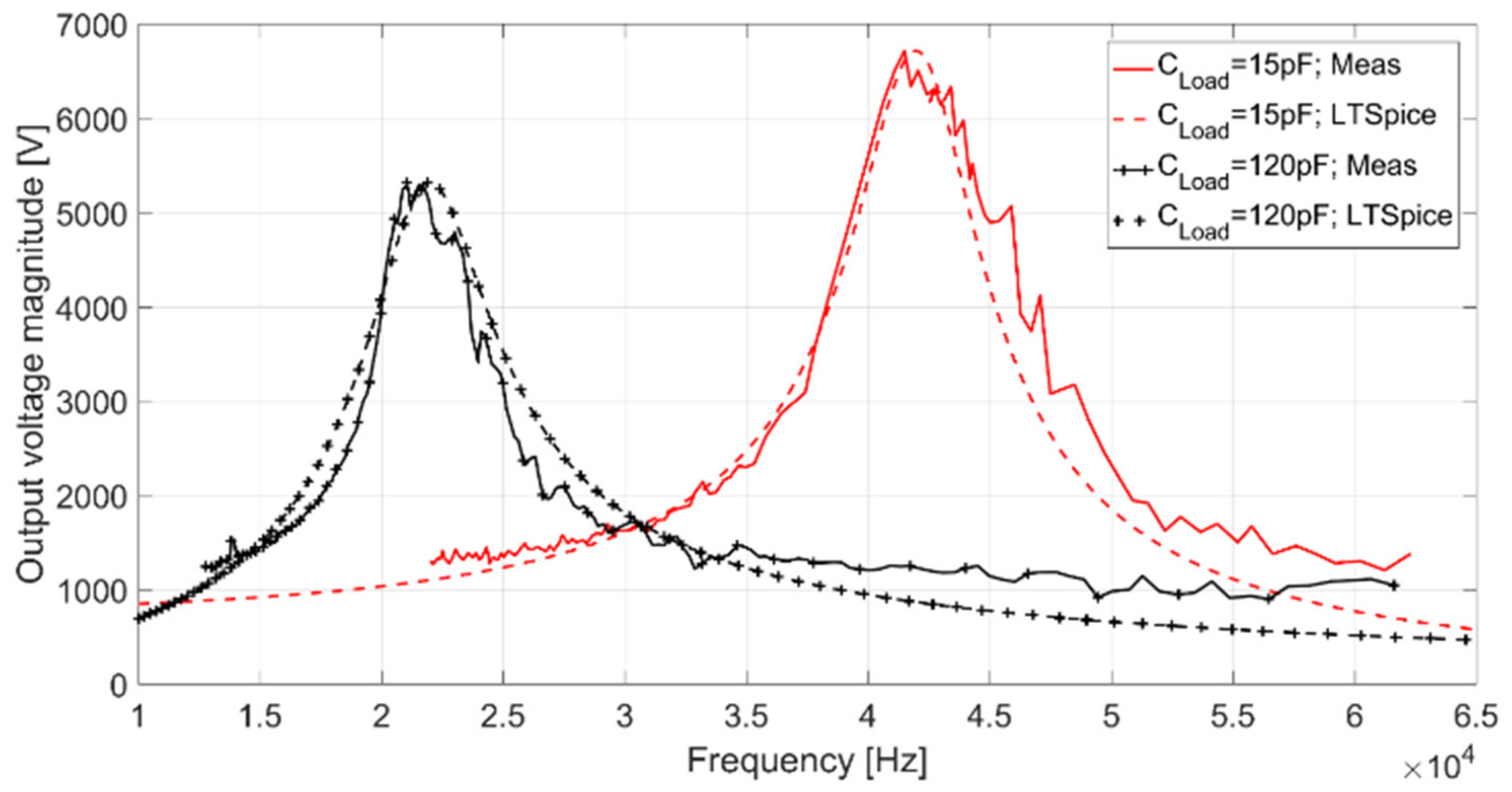
A first important aspect of this supply source is the dependence of the output voltage magnitude with respect to the switching frequency. This relation is shown in
Figure 8 when volumetric and surface reactors are supplied. The equivalent capacitance of the volumetric reactor is 120 pF and for the surface one is 15 pF. These values have been obtained by using the Asita AS250 impedance meter. Continuous lines refer to measurements done by means of the micro-controller, dashed lines are the LTspice simulation results.
Experimental results and simulations are in a very good agreement, underlying the validity of the simplified model used in LTspice. Depending on the load capacity, a different resonance frequency can be observed. As far as the transformation ratio of the transformer is about 143, at the resonance frequency the output voltage supplied by the generator strongly increases maintaining the same input DC voltage. As expected, by increasing the load capacitance both the resonance frequency and the output voltage decrease.
In
Figure 9a a comparison between measurements and simulation results is shown. On the left-hand side low voltage quantities as MOSFET voltages and bus DC current are shown. On the right-hand side output voltage is presented. This comparison is carried out for frequencies less than, equal to and greater than the soft switching frequency (
fss), at a fixed input DC voltage equal to 10 V and a reactor capacitance of 15 pF. As it has been shown for the results in
Figure 8, an overall good agreement between measurements and simulations have been obtained.
For
f = fss (
Figure 9b), MOSFET commutations take place when the bus DC current crosses zero (ZCS condition). Consequently, power dissipation during commutations is virtually avoided. Moreover, MOSFET overvoltages are minimized. For frequencies less than
fss (
Figure 9a) or greater than
fss (
Figure 9c), the bus DC current is forced toward the zero value. This generates commutation losses into the MOSFETs and severe overvoltages that must be limited by snubber circuits. The overvoltages can exceed the regime value by several times. As an example, in
Figure 10 the measured MOSFET voltages with and without the snubber circuit, for a frequency less than the soft switching value are plotted. Without the snubber circuit the overvoltage is about 5 times the regime value.
In the right-hand side of
Figure 9, the output voltage time behavior at three frequencies is shown. Again, a very good agreement between measurements and simulations has been obtained. When working with a frequency less than the soft switching frequency, the output voltage presents a high harmonic content. The harmonic distortion strongly decreases at the soft switching frequency and almost disappears when working beyond this value.
The working frequency influences the overall generator efficiency too. An evaluation of this important parameter, given by the ratio between the discharge average power and the DC input power, has been carried out. Both reactors already used to obtain the voltage frequency response presented in
Figure 8 have been utilized for this purpose. As already mentioned, the first reactor is a surface DBD with an equivalent load capacitance of 15 pF, the second one is a volumetric DBD with an equivalent capacitance of 120 pF. In order to maintain the average power feeding both discharges to a constant value, 170 W for the volumetric reactor and 12 W for the surface one, input DC voltage has been decreased by increasing the switching frequency. Average discharge power has been evaluated with the Q-V Lissajous technique mentioned above. For both reactors, switching frequency has been varied in a range comprising soft switching and resonance frequencies. Switching frequency has been varied with steps of 1 kHz, and according to results shown in
Figure 8, it has been increased from 27 to 44 kHz for the surface DBD reactor (15 pF equivalent load), and from 12 to 23 kHz for the volumetric one (120 pF equivalent load).
The generator efficiency as a function of the switching frequency is shown in
Figure 11 for both reactors. Soft switching and resonance frequency (
fss and
fres, respectively) are displayed in the figure for both reactors. The efficiency trend is quite similar for both loads. It is possible to notice that, by working below the soft switching value, quite low efficiency is measured. At the soft switching frequency, a considerable increase of the efficiency is achieved. By further increasing the switching frequency, a plateau of the efficiency value is reached. Then, approaching the resonance frequency, the efficiency decreases. At the resonance frequency a sudden decrease of the efficiency is obtained. By further increasing the frequency this low value is maintained.
A possible explanation of the efficiency trend, as a function of the working frequency can be given as follows. The main loss mechanisms are due to the Joule dissipation into windings and snubber components, and to iron losses. Below
fss, snubber and iron losses dominate because of the relevant MOSFET overvoltages suppressed by snubbers and the important harmonic content owned by the output voltage (see right-hand side of
Figure 9a). Working at
fss, both snubber and iron losses are strongly decreased. The Joule heating into windings starts to increase as the bus DC current increases. By a further increase of the frequency, iron losses decrease further as the output voltage’s maximum value and its harmonic content both decrease. Thus, the high efficiency plateau is achieved. With a working frequency close to
fres, a strong increase of the winding current occurs. Therefore, a considerable Joule heating is generated. For frequencies equal to or lower than
fres, the Joule heating into windings and snubber dominate the losses, leading to a severe efficiency decrement. Loss mechanisms already described can be considered to explain differences in the efficiency trends for the two reactors as well. When average power feeding the surface discharge is more than an order of magnitude lower with respect to that supplying volumetric reactor, it is possible to affirm that iron losses are predominant in the surface reactor, especially in the low frequency range. As a matter of fact, these losses are related with the applied voltage value and not related with the current flowing into windings. This consideration could explain the lower value in the high efficiency plateau observed beyond soft switching frequency. On a parallel plane the decrement in efficiency for the surface reactor does not take place in such an abrupt way as it happens for the volumetric discharge. This could be related to a lower Joule heating effect taking place in the windings because of the lower average power delivered to the surface DBD.
Figure 11 shows the optimal frequency range at which the generator works. This range is between 14–16 kHz for the volumetric reactor and between 30–34 kHz for the surface one, corresponding to the plateau with high efficiency. On the other hand, this range guarantees both limited MOSFET overvoltages and a low harmonic content of the supply output voltage (
Figure 9). The best working frequency, centered with respect to the high efficiency plateau region, can be found by means of the following empirical expression:
6. Self-Tuning Control Strategy
In the previous section the definition and the evaluation of the best working frequency has been defined. This value can be automatically selected following the control strategy described below.
When a new load is connected to high-voltage terminals, an input DC voltage less than 1 V is set. Thus, the micro-controller performs a frequency scan and measures the output voltage corresponding to each frequency. The low input DC voltage guarantees limited high-voltage values avoiding reactor damages. For each frequency, the maximum value of the output voltage, and the corresponding fast Fourier transform (FFT) of the signal are calculated. The maximal value of maximal voltages for all frequencies corresponds to the resonance frequency (see
Figure 7).
The FFT is calculated with a native Arduino library and allows finding the soft switching frequency. In the right-hand side of
Figure 9, output voltages with frequencies less than, equal to and greater than the soft switching value have been shown. Normalized FFTs of these signals, determined by means of the micro-controller, are displayed in
Figure 12.
The voltage harmonic content is higher for low frequencies and decreases approaching the resonance value. The ratio between first and third harmonic can be utilized by the micro-controller to determine the soft switching frequency. For the supply generator described in this work this ratio corresponds to 11.
The time used by the micro-controller for the frequency scan is about 5 s. After this procedure the soft switching frequency and the resonance frequency are known, and the micro-controller determines the best working frequency by means of the expression given in Equation (4).
After this initial self-tuning routine, the DC input is increased to reach the desired output voltage. The micro-controller measures the high voltage Vout obtained and charge Qm. Thus, the average power supplied to the discharge is calculated. About 5 ms, of which 2 ms are for the sampling procedure and 3 ms are for the calculations, are used for the evaluation of the average output power. Therefore, a quasi-real-time evaluation of most important parameters of the discharge are available for the user and the optimal frequency and working voltage can be utilized.


