Article

Spline Function Simulation Data Generation for Walking Motion Using Foot-Mounted Inertial Sensors

Electrical Engineering Department, University of Ulsan, Ulsan 44610, Korea
*
Author to whom correspondence should be addressed.
Electronics 2019, 8(1), 18; https://doi.org/10.3390/electronics8010018
Submission received: 22 October 2018 / Revised: 19 December 2018 / Accepted: 20 December 2018 / Published: 23 December 2018
(This article belongs to the Special Issue Sensing and Signal Processing in Smart Healthcare)

Abstract

:
This paper investigates the generation of simulation data for motion estimation using inertial sensors. The smoothing algorithm with waypoint-based map matching is proposed using foot-mounted inertial sensors to estimate position and attitude. The simulation data are generated using spline functions, where the estimated position and attitude are used as control points. The attitude is represented using B-spline quaternion and the position is represented by eighth-order algebraic splines. The simulation data can be generated using inertial sensors (accelerometer and gyroscope) without using any additional sensors. Through indoor experiments, two scenarios were examined include 2D walking path (rectangular) and 3D walking path (corridor and stairs) for simulation data generation. The proposed simulation data is used to evaluate the estimation performance with different parameters such as different noise levels and sampling periods.

Graphical Abstract

1. Introduction

Motion estimation using inertial sensors is one of the most important research topics that is increasingly applied in many application areas such as medical applications, sports, and entertainment [1]. Inertial measurement unit (IMU) sensors are commonly used to estimate human motion [2,3,4,5]. Inertial sensors can be used alone or combined with other sensors such as cameras [6,7] or magnetic sensors [8]. In personal navigation and healthcare applications [9,10,11], foot-mounted inertial sensors without using any additional sensors is a key enabling technology since it does not require any additional infrastructure. If additional sensors (other than inertial sensors) are also used, sensor fusion algorithms [12,13] can be used to obtain more accurate motion estimation.
To evaluate the accuracy of any motion estimation algorithm, it is necessary to compare the estimated value with the true value. The estimated value is usually verified through experiments with both IMU and optical motion tracker [14,15]. In [2], the Vicon optical motion capture system is used to evaluate the effectiveness of human pose estimation method and its associated sensor calibration procedure. An optical motion tracking is used as a reference to compare with motion estimation using inertial sensors in [15].
Although the experimental validation gives the ultimate proof, it is not only more convenient but also more important to work with simulation data, which is statistically much more relevant for testing and the development of algorithms. For example, the effect of gyroscope bias on the performance of an algorithm cannot be easily identified in experiments. In this case, simulation using synthesized data is more convenient since gyroscope bias can be changed arbitrarily.
In [16,17,18], IMU simulation data are generated using optical motion capture data for human motion estimation. In [19], IMU simulation data is generated for walking motion by approximating walking trajectory as simple sinusoidal functions. In [20,21,22], IMU simulation data are also generated for flight motion estimation using an artificially generated trajectory. There are many different methods to represent attitude and position simulation data. Among them, the spline function is the most popular approach [23]. The B-spline quaternion algorithm provides a general curve construction scheme that extends the spline curves [24]. Reference [25] presents an approach for attitude estimation using cumulative B-splines unit quaternion curves. Position can be represented by any spline function [23]. Usually, position data are represented using cubic spline functions. The cubic spline function gives a continuous position, velocity, and acceleration. However, the acceleration is not sufficiently smooth. This is a problem for the inertial sensor simulation data generation since the smooth accelerometer data cannot be generated. Thus, we use the eighth-order spline function for position data since it gives position data with smooth acceleration, whose jerk (third derivative) can be controlled in the optimization problem.
In this paper, we use cumulative B-spline for attitude representation and eighth-order algebraic spline for position representation. The eighth-order algebraic spline is a slightly modified version of the spline function from a previous study [26].
The aim of this paper is to obtain simulation data combining inertial sensors (accelerometer and gyroscope) and waypoint data without using any additional sensors. A computationally efficient waypoint-based map matching smoothing algorithm is proposed for position and attitude estimation from foot-mounted inertial sensors. The simulation data are generated using spline functions, where the estimated position and attitude are used as control points. This paper is an extended version of a work published in the conference paper [27], where a basic algorithm with a simple experimental result is given.
The remainder of the paper is organized as follows. Section 2 describes the smoothing algorithm with waypoint-based map matching to estimate motion for foot-mounted inertial sensors. Section 3 describes the computation of the spline function to generate simulation data. Section 4 provides the experiment results to verify the proposed method. Conclusions are given in Section 5.

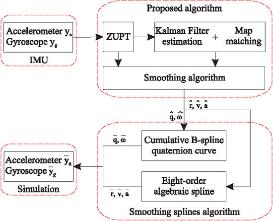
2. Smoothing Algorithm with Waypoint-Based Map Matching

In this section, a smoothing algorithm is proposed to estimate the attitude, position, velocity and acceleration, which will be used to generate simulation data in Section 3.
Two coordinate frames are used in this paper: the body coordinate frame and the navigation coordinate frame. The three axes of the body coordinate frame coincide with the three axes of the IMU. The z axis of the navigation coordinate frame coincides with the local gravitational direction. The choice of the x and y axes of the navigation coordinate frame can be arbitrarily chosen. The notation [ p ] n ( [ p ] b ) is used to denote that a vector p is represented in the navigation (body) coordinate frame.
The position is defined by [ r ] n R 3 , which is the origin of the body coordinate frame expressed in the navigation coordinate frame. Similarly, the velocity and the acceleration are denoted by [ v ] n R 3 and [ a ] n R 3 , respectively. The attitude is represented using a quaternion q R 4 , which represents the rotation relationship between the navigation coordinate frame and the body coordinate frame. The directional cosine matrix corresponding to quaternion q is denoted by C ( q ) S O ( 3 ) .
The accelerometer output y a R 3 and the gyroscope output y g R 3 are given by
y a = C ( q ) g ˜ + a b + n a , y g = ω + n g ,
where ω R 3 is the angular velocity, a b R 3 is the external acceleration (acceleration related to the movement, excluding the gravitational acceleration) expressed in the body coordinate frame, and n a R 3 and n g R 3 are sensor noises. The vector g ˜ is the local gravitational acceleration vector. It is assumed that g ˜ is known, which can be computed using the formula in [28]. The sensor biases are assumed to be estimated separately using calibration algorithms [29,30].
Let T denote the sampling period of a sensor. For a continuous time signal y ( t ) , the discrete value is denoted by y k = y ( k T ) . The discrete sensor noise n a , k and n g , k are assumed to be white Gaussian sensor noises, whose covariances are given by
R a = E n a , k n a , k T = r a I 3 R 3 × 3 , R g = E n g , k n g , k T = r g I 3 R 3 × 3 .
where r a > 0 and r g > 0 are scalar constants.
We assume that a walking trajectory consists of straight line paths, where the angle between two adjacent paths can only take one of the following angle { 90 , 90 , 180 } . An example of a walking trajectory is given in Figure 1, where there is 90 turn at P 2 and 90 turn at P 3 . Waypoints are denoted by P m R 3 ( 1 m M ), which include positions with turn events ( P 2 and P 3 in Figure 1), the initial position ( P 1 ) and the final position ( P 4 ).

2.1. Standard Inertial Navigation Using an Indirect Kalman Filter

In this subsection, q, r, and v are estimated using a standard inertial navigation algorithm with an indirect Kalman filter [31].
The basic equations for inertial navigation are given as follows:
q ˙ = 1 2 Ω ( ω ) q , v ˙ n = a n = C T ( q ) a b , r ˙ n = v n ,
where symbol Ω is defined by
Ω ( ω ) = 0 ω T ω [ ω × ] ,
and [ ω × ] R 3 × 3 denotes the skew symmetric matrix of ω :
[ ω × ] = 0 ω z ω y ω z 0 ω x ω y ω x 0 .
Let q ^ k , r ^ k and v ^ k be the estimated values of q, r and v using (3), where ω and a b are replaced by y g and y a C ( q ^ ) g ˜ :
q ^ ˙ = 1 2 Ω ( y g ) q ^ , v ^ ˙ = C T ( q ^ ) y a g ˜ , r ^ ˙ = v ^ .
Coriolis and Earth curvature effects are ignored since we use a consumer grade IMU for limited walking distances where these effects are below the IMU noise level [32].
When the initial attitude ( q ^ 0 ) is computed, the pitch and roll angles can be computed from y a , 0 . However, the yaw angle is not determined since there is no heading reference sensor such as a magnetic sensor. In the proposed algorithm, the initial yaw angle can be arbitrarily chosen since the yaw angle is automatically adjusted later (see Section 2.3).
q ¯ e , r e and v e denote the estimation errors in q ^ , r ^ , and v ^ , which are defined by
q ¯ e q q ^ k * , r e r n r ^ k , v e v n v ^ k ,
where ⊗ is the quaternion multiplication and q * denotes the quaternion conjugate of a quaternion q. Assuming that q ¯ e is small, we can approximate q ¯ e as follows:
q ¯ e 1 q e .
The state of an indirect Kalman filter is defined by
x q e r e v e R 9 × 1 .
The state equation for the Kalman filter is given by [31]:
x ˙ = [ y g × ] 0 0 0 0 I 3 2 C ( q ^ ) T [ y a × ] 0 0 x + w
where the covariance of the process noise w is given by
E w w T = 0 . 25 R g 0 0 0 0 0 0 0 C ( q ^ ) T R a C ( q ^ ) .
The discretized version of (8) is used in the Kalman filter as in [31].
Two measurement equations are used in the Kalman filter: the zero velocity updating (ZUPT) equation and the map matching equation.
The zero velocity updating uses the fact that there is almost periodic zero velocity intervals (when a foot is on the ground) during walking. If the following conditions are satisfied, the discrete time index k is assumed to belong to zero velocity intervals [31]:
y g , i B g , k N g 2 i k + N g 2 y a , i y a , i 1 B a , k N a 2 i k + N a 2
where B g , B a , N g and N a are parameters for zero velocity interval detection. This zero velocity updating algorithm is not valid when a person is on a moving transportation such as an elevator. Thus, the proposed algorithm cannot be used when a person is on a moving transportation.
During the zero velocity intervals, the following measurement equation is used:
0 3 × 1 v ^ k = 0 3 × 3 0 3 × 3 I 3 x k + n v ,
where n v is a fictitious measurement noise representing a Gaussian white noise with the noise covariance R v .
The second measurement equation is from the map matching, which is used during the zero velocity intervals. From the assumption, a straight line path is parallel to either x axis or y axis. If a path is parallel to x ( y ) axis, y ( x ) position is constant and this can be used in the measurement equation.
Let e i R 3 × 1 ( 1 i 3 ) be the unit vector whose i-th element is 1 and the remaining elements are 0. Suppose a person is on the path [ P m , P m + 1 ] and
e j T ( P m + 1 P m ) = 0 , j = 1 or 2 .
For example, (11) is satisfied with j = 1 if the path is parallel to the y axis.
When (11) is satisfied with j ( j = 1 or 2 ), then the map matching measurement equation is given by
e j T ( P m r ^ k ) = 0 1 × 3 e j T 0 1 × 3 x k + n r , 12 ,
where n r , 12 is the horizontal position measurement noise whose noise covariance is R r , 12 .
If the path is level (that is, e 3 T ( P m + 1 P m ) = 0 ), the z axis value of r k is almost the same in the zero velocity intervals when the foot is on the ground. In this case, the following z axis measurement equation is also used:
e 3 T ( P m r ^ k ) = 0 1 × 3 e 3 T 0 1 × 3 x k + n r , 3 ,
where n r , 3 is the vertical position measurement noise whose noise covariance is R r , 3 .
The proposed filtering algorithm is illustrated in Figure 2. To further reduce the estimation errors of the Kalman filter, the smoothing algorithm in [31] is applied to the Kalman filter estimated values.

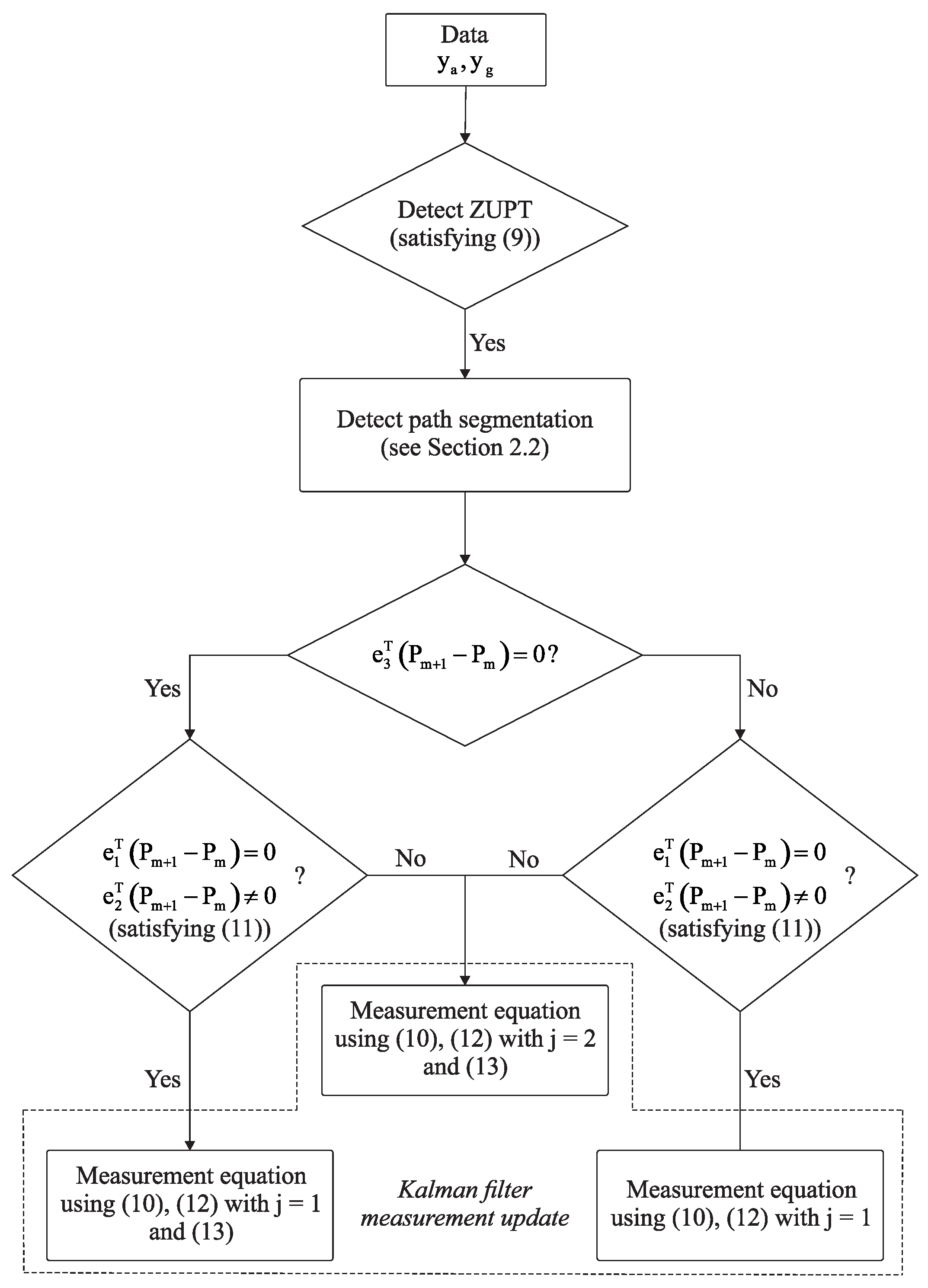
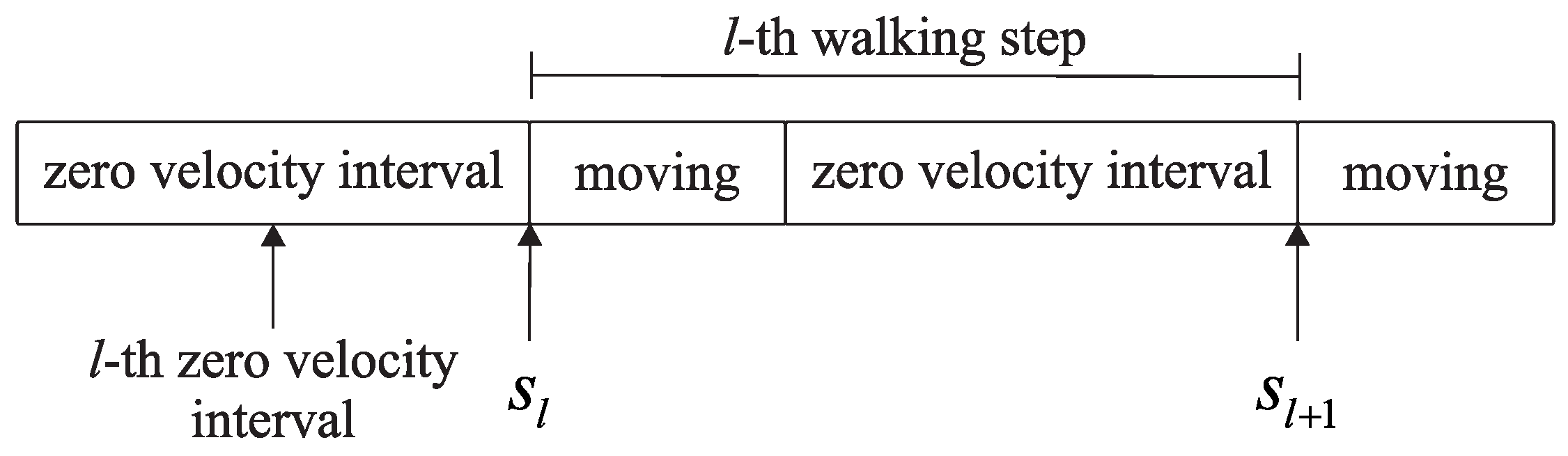
2.2. Path Identification

To apply map matching measurement Equation (12), a current path must be identified. Using the zero velocity intervals, each walking step can be easily determined. Let S l be the discrete time index of the end of l-th zero velocity interval (see Figure 3).
Let ψ S l be the yaw angle at the discrete time S l and ψ l be defined by
ψ l ψ S l + 1 ψ S l .
Please note that ψ l denotes the yaw angle change during l-th walking step.
The turning (that is, the change of a path) is detected using ψ l . Suppose a current path is [ P m , P m + 1 ] . Then the next turning angle is determined by two vectors P m + 1 P m and P m + 2 P m + 1 . For example in Figure 1, if a current path is [ P 1 , P 2 ] , the next turning angle is 90 . Let δ be the next turning angle. Turning is determined to occur at l-th walking step if the following condition is satisfied:
j = l M l l + M l ψ j δ < ψ th ,
where ψ th is a threshold parameter and M l is a positive integer parameter. Equation (15) detects the turning if the summation of the yaw angle changes during 2 M l + 1 walking steps is similar to the next expected turning angle δ . The use of parameter M l is due to the fact that turning does not occur during a single step. Once turning is detected in (15), a current path is modified to [ P m + 1 , P m + 2 ] from [ P m , P m + 1 ] .

2.3. Initial Yaw Angle Adjustment

The initial yaw angle is arbitrarily chosen and adjusted as follows. Suppose the first N first walking steps belong to the first path [ P 1 , P 2 ] . Let x l and y l ( 1 l N l ) be defined by
x l y l = e 1 T e 2 T r ^ S l , 1 l N l .
The line equation representing ( x l , y l ) is computed using the following least squares optimization:
min a , b , c l = 1 N l a x l + b y l + c 2 2 .
The angle between the line (defined by the line equation a, b, c) and [ e 1 e 2 ] T ( P 2 P 1 ) is computed. Using this angle, the initial yaw angle is adjusted so that the walking direction coincides with the direction dictated by the waypoints.

3. Spline Function Computation

In this section, spline function q ¯ ( t ) (quaternion spline) and r ¯ ( t ) (position spline) are computed using q ^ k , r ^ k and v ^ k as control points.

3.1. Cumulative B-Splines Quaternion Curve

Since the quaternion spline q ¯ ( t ) is computed for each interval [ k T , ( k + 1 ) T ) , it is convenient to introduce q ¯ k ( u ) notation, which is defined by
q ¯ ( t ) = q ¯ k ( u ) q ¯ ( k T + u ) , t [ k T , ( k + 1 ) T ) , 0 u < T .
To define q ¯ k ( u ) , ω ^ k is defined as follows:
ω ^ k 1 T log ( C ( q ^ k + 1 ) C T ( q ^ k ) ) ,
where the logarithm of an orthogonal matrix is defined in [33]. Please note that w ^ k is a constant angular velocity vector, which transform from q ^ k to q ^ k + 1 .
Cumulative B-spline basis function is used to represent the quaternion spline, which is first proposed in [24] and also used in [34].
q ¯ k ( u ) = ( i = 1 3 S i ( u ) ) q ^ k 1
where
S i ( u ) exp ( 1 2 B ˜ i ( u ) Ω ( ω ^ k 2 + i ) ) .
The cumulative basis function B ˜ i ( u ) R 3 ( 1 i 3 ) is defined by
B ˜ 1 ( u ) B ˜ 2 ( u ) B ˜ 3 ( u ) = D 1 u T u 2 T 2 u 3 T 3
where D is computed using the matrix representation of the De Boor–Cox formula [34]:
D = 1 6 5 3 3 1 1 3 3 2 0 0 0 1 .
To generate the gyroscope simulation data, the angular velocity spline ω ¯ ( t ) is required. From the relationship between q ¯ ( t ) and ω ¯ ( t ) [35], ω ¯ ( t ) is given by
ω ¯ ( t ) = 2 Ξ ( q ¯ ( t ) ) q ¯ ˙ ( t )
where
Ξ ( q ) q 1 q 2 q 3 q 0 q 3 q 2 q 3 q 0 q 1 q 2 q 1 q 0 .
The derivative of q ¯ ( t ) ( k T t < ( k + 1 ) T ) is given by
q ¯ ˙ ( t ) = d q ¯ k ( u ) d u = ( S ˙ 3 S 2 S 1 + S 3 S ˙ 2 S 1 + S 3 S 2 S ˙ 1 ) q ^ k 1
where
S ˙ i = d S i ( u ) d u = 1 2 B ˜ ˙ i ( u ) Ω ( ω ^ k 2 + i ) S i
B ˜ ˙ ( u ) = B ˜ ˙ 1 ( u ) B ˜ ˙ 2 ( u ) B ˜ ˙ 3 ( u ) = D 0 1 T 2 u T 2 3 u 2 T 3 .

3.2. Eighth-Order Algebraic Splines

The position r ¯ ( t ) is represented by eighth-order algebraic spline [26], where k-th spline segment is given by
r ¯ ( t ) = r ¯ k , m ( u ) = j = 0 7 p k j , m u j , t [ k T , ( k + 1 ) T ) .
where p k j , m ( 0 k N , 0 j 7 , 1 m 3 ) are the coefficients of the k-th spline segment of the m-th element of r ¯ k (for example, r ¯ k , 1 is the x position spline). Continuity constraints up to third derivative of r ¯ k , m ( u ) are imposed on the coefficients.
Let a ^ k be the estimated value of the external acceleration in the navigation coordinate frame, which can be computed as follows (see (3))
a ^ k = C T ( q ^ k ) y a , k g ˜ .
The coefficients p k j , m are chosen so that r ¯ ( k T ) , r ¯ ˙ ( k T ) and r ¯ ¨ ( k T ) are close to r ^ k , v ^ k and a ^ k . An additional constraint is also imposed to reduce the jerk term (the third derivative of r ¯ ( t ) ), which makes r ¯ ( t ) smooth rather than jerky. Thus, the performance index for m-th element ( 1 m 3 ) of r ¯ ( t ) is defined as follows:
J m = α 1 k = 0 N ( r ¯ k , m ( T ) r ^ k , m ) 2 + α 2 k = 0 N ( r ¯ ˙ k , m ( T ) v ^ k , m ) 2 + α 3 k = 0 N ( r ¯ ¨ k , m ( T ) a ^ k , m ) 2 + β k = 0 N 0 T ( r ¯ k , m ( t ) ) 2 d t .
This minimization of J m can be formulated as a quadratic minimization problem of the coefficients p k j , m as follows:
min X J m = X T M 1 X + 2 M 2 X + M 3
where M 1 R 8 ( N 1 ) × 8 ( N 1 ) , M 2 R 1 × 8 ( N 1 ) and M 3 R can be computed from (26).
Although the matrix size of M 1 could be large, it is a banded matrix with a bandwidth of 7. An efficient Cholesky decomposition algorithm is available for matrices with a small bandwidth [36] and (27) can be solved efficiently.
Let p ¯ k j , m be the minimization solution of (26). Then r ¯ can be computed by inserting p ¯ k j , m into (24) and v ¯ , a ¯ can be computed by taking the derivatives.
The weighting factors α i ( 1 i 3 ) and β determine the smoothness of r ¯ , v ¯ and a ¯ . If β is large, we obtain smoother r ¯ , v ¯ and a ¯ curves at the sacrifice of nearness to the control points r ^ , v ^ and a ^ .
Let y ¯ a and y ¯ g be accelerometer and gyroscope output generated using the spline functions. These values can be generated using (1), where q, a b , ω are replaced by q ¯ , C ( q ¯ ) a ¯ , ω ¯ with appropriate sensor noises. An overview of the simulation data generation system is shown in Figure 4.

4. Experiment and Results

In this section, the proposed algorithm is implemented through indoor experiments. An inertial measurement unit MTi-1 of XSens was attached on the foot with the sampling frequency of 100 Hz. The parameters used in the proposed algorithm are given in Table 1.
Two experiment sets of scenarios are conducted: (1) walking along a rectangular path for 2D walking data generation; and (2) walking on corridors and stairs for 3D walking data generation.

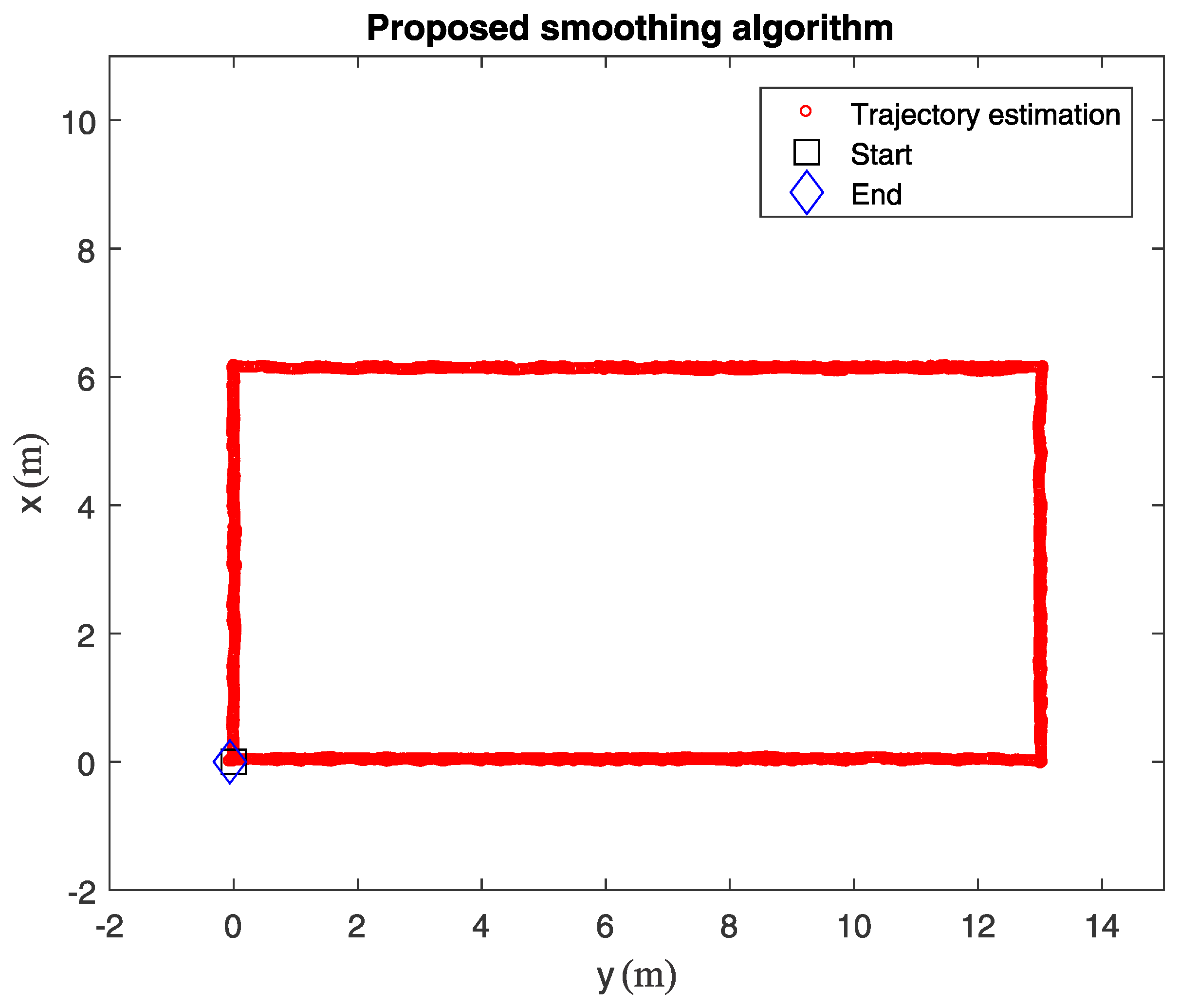
4.1. Walking along a Rectangular Path

In this experimental scenario, the subjects walked five laps at normal speed along a rectangular path with dimensions of 13.05 m by 6.15 m. The total distance for five laps on the path was 192 m.
The standard Kalman filter results without map matching are given in Figure 5. The errors in Figure 5 were primarily driven by the errors in the orientation estimation as well as run bias instability of the inertial sensors leading to the position error of 1 m. As can be seen that the maximum error was almost 2 m at the end of the walking.
The navigation results in Figure 6 were obtained from the proposed smoothing algorithm with map matching. It can be seen that the results are improved due to the map matching.
The z axis spline data (for the three walking steps out of the rectangle walking steps) is given in Figure 7.

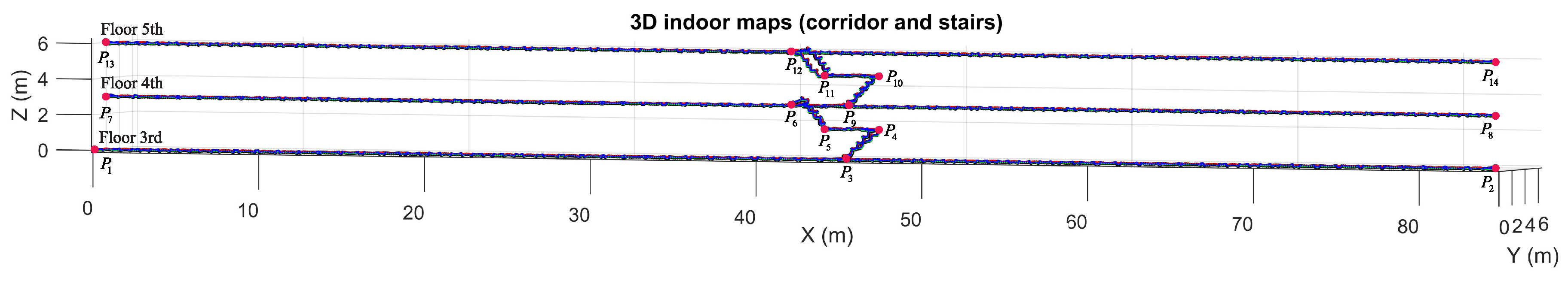
4.2. Walking along a 3D Indoor Environment

In the second experimental scenario, a person walked along a 3D indoor environment corridors and stairs.
Figure 8 shows the walking along a 3D trajectory results with a waypoint P 1 is the starting point whose coordinate is ( 0 , 0 , 0 ) . The coordinates of waypoints P 1 to P 14 are known, and the starting waypoint P 1 coincides with the end waypoint P 14 on the projection plane. The routes are as follow: starting from the third floor waypoint P 1 , walking along the floor to collect data with normal speed then turning 180 in P 2 and turning on the right in P 3 , then going up the stairs through the floor by the same way as the other floors, finally reaching the fifth floor waypoint P 14 , after that turning 180 and walking along the floor to coming back the starting waypoint P 1 . The total length of the path line is approximately 562.98 m.

4.3. Evaluation of Simulation Data Usefulness

The simulation data used to test specific performance of a certain algorithm. In this subsection, the standard Kalman filter without map matching is evaluated using the simulation data generated in Section 4.1. The algorithm is tested 1000 times with different noise values (walking motion data is the same).
Let r ¯ x y , final , i be the estimation error of the final position value (x and y components) of i-th simulation, where 1 i 1000 . Since the mean value of r ¯ x y , final , i is not exactly zeros, its mean value is subtracted.
The accuracy of an algorithm can be evaluated from the distribution of r ¯ x y , final , i . Consider an ellipse whose center point is the mean of r ¯ x y , final , i and which include 50% of r ¯ x y , final , i (see Figure 9). Let a be the length of the major axis and b be the length of the minor axis. Smaller values of a and b indicate that the error of a certain algorithm is smaller.

4.3.1. Affects of Sampling Rate on the Estimation Performance

The simulation results for the final position estimated errors with different sampling rates are given in Table 2. As an example, Figure 9 shows the estimation error of the final position value with a sampling rate of 100 Hz, where an ellipse represents the boundary of 50% of probability. As can be seen, the final position errors of the different sampling rates are almost the same except for the result with a sampling rate of 50 Hz. This simulation result suggests that the sampling rate is smaller than 100 Hz is not desirable. Also, there is no apparent benefit using the sampling rate higher than 100 Hz.

4.3.2. Gyroscope Bias Effect

The simulation results for the final position estimated errors with different gyroscope bias are given in Table 3. As can be seen, the final position errors change significantly when the gyroscope bias becomes to change larger.

5. Conclusions

In this paper, simulation data is generated for walking motion estimation using inertial sensors. The first step to generate simulation data is to perform a specific motion, which you want to estimate. The attitude and position are computed from inertial sensors data using a smoothing algorithm. The spline functions are generated using the smoother estimated values as control points. B-spline function is used for the attitude quaternion, and eighth-order algebraic spline function is used for the position.
The spline simulation data generated from the proposed algorithm can be used to test a new motion estimation algorithm by easily changing the parameters such as noise covariance, sampling rate and bias terms.
The shape of generated spline function depends on the weighting factors, which control the constraint on the jerk term. It is one of future research topic to investigate how to choose the optimal weighting factors, which give the most realistic simulation data.

Author Contributions

T.T.P. and Y.S.S. conceived and designed this study. T.T.P. performed the experiments and wrote the paper. Y.S.S. reviewed and edited the manuscript.

Funding

This work was supported by the 2018 Research Fund of University of Ulsan.

Conflicts of Interest

The authors declare no conflict of interest.

References

  1. Zhou, H.; Hu, H. Human motion tracking for rehabilitation—A survey. Biomed. Signal Process. Control 2008, 3, 1–18. [Google Scholar] [CrossRef] [Green Version]
  2. Tao, Y.; Hu, H.; Zhou, H. Integration of vision and inertial sensors for 3D arm motion tracking in home-based rehabilitation. Int. J. Robot. Res. 2007, 26, 607–624. [Google Scholar] [CrossRef]
  3. Raiff, B.R.; Karataş, Ç.; McClure, E.A.; Pompili, D.; Walls, T.A. Laboratory validation of inertial body sensors to detect cigarette smoking arm movements. Electronics 2014, 3, 87–110. [Google Scholar] [CrossRef] [PubMed]
  4. Fang, T.H.; Park, S.H.; Seo, K.; Park, S.G. Attitude determination algorithm using state estimation including lever arms between center of gravity and IMU. Int. J. Control Autom. Syst. 2016, 14, 1511–1519. [Google Scholar] [CrossRef]
  5. Ahmed, H.; Tahir, M. Improving the accuracy of human body orientation estimation with wearable IMU sensors. IEEE Trans. Instrum. Meas. 2017, 66, 535–542. [Google Scholar] [CrossRef]
  6. Suh, Y.S.; Phuong, N.H.Q.; Kang, H.J. Distance estimation using inertial sensor and vision. Int. J. Control Autom. Syst. 2013, 11, 211–215. [Google Scholar] [CrossRef]
  7. Erdem, A.T.; Ercan, A.Ö. Fusing inertial sensor data in an extended Kalman filter for 3D camera tracking. IEEE Trans. Image Process. 2015, 24, 538–548. [Google Scholar] [CrossRef] [PubMed]
  8. Zhang, Z.; Meng, X. Use of an inertial/magnetic sensor module for pedestrian tracking during normal walking. IEEE Trans. Instrum. Meas. 2015, 64, 776–783. [Google Scholar] [CrossRef]
  9. Ascher, C.; Kessler, C.; Maier, A.; Crocoll, P.; Trommer, G. New pedestrian trajectory simulator to study innovative yaw angle constraints. In Proceedings of the 23rd International Technical Meeting of the Satellite Division of the Institute of Navigation (ION GNSS 2010), Portland, OR, USA, 21–24 September 2010; pp. 504–510. [Google Scholar]
  10. Jiménez, A.R.; Seco, F.; Prieto, J.C.; Guevara, J. Indoor pedestrian navigation using an INS/EKF framework for yaw drift reduction and a foot-mounted IMU. In Proceedings of the 7th Workshop on Positioning, Navigation and Communication, Dresden, Germany, 11–12 March 2010; pp. 135–143. [Google Scholar] [CrossRef]
  11. Fourati, H. Heterogeneous data fusion algorithm for pedestrian navigation via foot-mounted inertial measurement unit and complementary filter. IEEE Trans. Instrum. Meas. 2015, 64, 221–229. [Google Scholar] [CrossRef]
  12. Rodger, J.A. Toward reducing failure risk in an integrated vehicle health maintenance system: A fuzzy multi-sensor data fusion Kalman filter approach for IVHMS. Expert Syst. Appl. 2012, 39, 9821–9836. [Google Scholar] [CrossRef]
  13. He, C.; Kazanzides, P.; Sen, H.T.; Kim, S.; Liu, Y. An Inertial and Optical Sensor Fusion Approach for Six Degree-of-Freedom Pose Estimation. Sensors 2015, 15, 16448–16465. [Google Scholar] [CrossRef] [PubMed] [Green Version]
  14. Kim, A.; Golnaraghi, M.F. Initial calibration of an inertial measurement unit using an optical position tracking system. In Proceedings of the PLANS 2004. Position Location and Navigation Symposium (IEEE Cat. No.04CH37556), Monterey, CA, USA, 26–29 April 2004; pp. 96–101. [Google Scholar] [CrossRef]
  15. Enayati, N.; Momi, E.D.; Ferrigno, G. A quaternion-based unscented Kalman filter for robust optical/inertial motion tracking in computer-assisted surgery. IEEE Trans. Instrum. Meas. 2015, 64, 2291–2301. [Google Scholar] [CrossRef]
  16. Karlsson, P.; Lo, B.; Yang, G.Z. Inertial sensing simulations using modified motion capture data. In Proceedings of the 11th International Conference on Wearable and Implantable Body Sensor Networks (BSN 2014), ETH Zurich, Switzerland, 16–19 June 2014. [Google Scholar]
  17. Young, A.D.; Ling, M.J.; Arvind, D.K. IMUSim: A simulation environment for inertial sensing algorithm design and evaluation. In Proceedings of the 10th ACM/IEEE International Conference on Information Processing in Sensor Networks, Chicago, IL, USA, 12–14 April 2011; pp. 199–210. [Google Scholar]
  18. Ligorio, G.; Sabatini, A.M. A simulation environment for benchmarking sensor fusion-based pose estimators. Sensors 2015, 15, 32031–32044. [Google Scholar] [CrossRef] [PubMed]
  19. Zampella, F.J.; Jiménez, A.R.; Seco, F.; Prieto, J.C.; Guevara, J.I. Simulation of foot-mounted IMU signals for the evaluation of PDR algorithms. In Proceedings of the 2011 International Conference on Indoor Positioning and Indoor Navigation, Guimaraes, Portugal, 21–23 September 2011; pp. 1–7. [Google Scholar] [CrossRef]
  20. Parés, M.; Rosales, J.; Colomina, I. Yet Another IMU Simulator: Validation and Applications; EuroCow: Castelldefels, Spain, 2008; Volume 30. [Google Scholar]
  21. Zhang, W.; Ghogho, M.; Yuan, B. Mathematical model and matlab simulation of strapdown inertial navigation system. Model. Simul. Eng. 2012, 2012, 264537. [Google Scholar] [CrossRef]
  22. Parés, M.E.; Navarro, J.A.; Colomina, I. On the generation of realistic simulated inertial measurements. In Proceedings of the 2015 DGON Inertial Sensors and Systems Symposium (ISS), Karlsruhe, Germany, 22–23 September 2015; pp. 1–15. [Google Scholar] [CrossRef]
  23. Schumaker, L. Spline Functions: Basic Theory, 3rd ed.; Cambridge Mathematical Library, Cambridge University Press: Cambridge, UK, 2007. [Google Scholar]
  24. Kim, M.J.; Kim, M.S.; Shin, S.Y. A general construction scheme for unit quaternion curves with simple high order derivatives. In Proceedings of the 22nd Annual Conference on Computer Graphics and Interactive Techniques, Los Angeles, CA, USA, 6–11 August 1995; ACM: New York, NY, USA, 1995; pp. 369–376. [Google Scholar] [CrossRef] [Green Version]
  25. Sommer, H.; Forbes, J.R.; Siegwart, R.; Furgale, P. Continuous-time estimation of attitude using B-Splines on Lie groups. J. Guid. Control Dyn. 2016, 39, 242–261. [Google Scholar] [CrossRef]
  26. Simon, D. Data smoothing and interpolation using eighth-order algebraic splines. IEEE Trans. Signal Process. 2004, 52, 1136–1144. [Google Scholar] [CrossRef]
  27. Pham, T.T.; Suh, Y.S. Spline function simulation data generation for inertial sensor-based motion estimation. In Proceedings of the 2018 57th Annual Conference of the Society of Instrument and Control Engineers of Japan (SICE), Nara, Japan, 11–14 September 2018; pp. 1231–1234. [Google Scholar]
  28. Pavlis, N.K.; Holmes, S.A.; Kenyon, S.C.; Factor, J.K. The development and evaluation of the Earth Gravitational Model 2008 (EGM2008). J. Geophys. Res. Solid Earth 2012, 117. [Google Scholar] [CrossRef] [Green Version]
  29. Metni, N.; Pflimlin, J.M.; Hamel, T.; Souères, P. Attitude and gyro bias estimation for a VTOL UAV. Control Eng. Pract. 2006, 14, 1511–1520. [Google Scholar] [CrossRef]
  30. Hwangbo, M.; Kanade, T. Factorization-based calibration method for MEMS inertial measurement unit. In Proceedings of the 2008 IEEE International Conference on Robotics and Automation, Pasadena, CA, USA, 19–23 May 2008; pp. 1306–1311. [Google Scholar] [CrossRef]
  31. Suh, Y.S. Inertial sensor-based smoother for gait analysis. Sensors 2014, 14, 24338–24357. [Google Scholar] [CrossRef]
  32. Placer, M.; Kovačič, S. Enhancing indoor inertial pedestrian navigation using a shoe-worn marker. Sensors 2013, 13, 9836–9859. [Google Scholar] [CrossRef]
  33. Gallier, J.; Xu, D. Computing exponential of skew-symmetric matrices and logarithms of orthogonal matrices. Int. J. Robot. Autom. 2002, 17, 1–11. [Google Scholar]
  34. Patron-Perez, A.; Lovegrove, S.; Sibley, G. A spline-based trajectory representation for sensor fusion and rolling shutter cameras. Int. J. Comput. Vis. 2015, 113, 208–219. [Google Scholar] [CrossRef]
  35. Markley, F.L.; Crassidis, J.L. Fundamentals of Spacecraft Attitude Determination and Control; Springer: New York, NY, USA, 2014. [Google Scholar]
  36. Golub, G.H.; Van Loan, C.F. Matrix Computations; Johns Hopkins University Press: Baltimore, MD, USA, 1983. [Google Scholar]
Figure 1. Example of waypoints ( P 1 P 4 ).
Electronics 08 00018 g001
Figure 2. Proposed measurement update flowchart.
Electronics 08 00018 g002
Figure 3. Walking step segmentation.
Electronics 08 00018 g003
Figure 4. System overview for simulation data generation.
Electronics 08 00018 g004
Figure 5. Rectangle walking estimation for five laps using a standard Kalman filter.
Electronics 08 00018 g005
Figure 6. Rectangle walking estimation for five laps using the proposed smoothing algorithm.
Electronics 08 00018 g006
Figure 7. z axis spline functions of the rectangle walking.
Electronics 08 00018 g007
Figure 8. 3D path indoor estimation with the proposed smoothing algorithm.
Electronics 08 00018 g008
Figure 9. Estimation error of the final position value with a sampling rate 100 Hz [ellipse with 50% of probability radius].
Electronics 08 00018 g009
Table 1. Parameters used in the proposed algorithm
ParametersValuesRelated Equations
r a 0.0015(2)
r g 0.00001
B g 0.8(9)
B a 1.5
N g , N a 30
n v 0.01(10)
n r , 12 0.0004(12)
n r , 3 0.0004(13)
ψ th 30 (15)
α 1 , α 2 , α 3 1(26)
β 0.00001
Table 2. Final position errors with different sampling rates.
Sampling RateMean of r ¯ xy , final (m)Radius (m)
x ¯ final y ¯ final ab
50 Hz−1.5217−0.54280.76050.0215
100 Hz0.66390.47450.05540.0034
150 Hz0.69550.45580.05940.0032
200 Hz0.71560.45200.05820.0042
Table 3. Final position errors with different gyroscope bias.
r g Mean of r ¯ xy , final (m)Radius (m)
x ¯ final y ¯ final ab
00.70230.61220.1330.0226
0.000010.65680.46960.05950.0035
0.0001−0.2038−0.02800.59520.0309
0.001−6.37680.55683.51231.0306

