A Deep Feature Extraction Method for HEp-2 Cell Image Classification

Abstract

The automated and accurate classification of the images portraying the Human Epithelial cells of type 2 (HEp-2) represents one of the most important steps in the diagnosis procedure of many autoimmune diseases. The extreme intra-class variations of the HEp-2 cell images datasets drastically complicates the classification task. We propose in this work a classification framework that, unlike most of the state-of-the-art methods, uses a deep learning-based feature extraction method in a strictly unsupervised way. We propose a deep learning-based hybrid feature learning with two levels of deep convolutional autoencoders. The first level takes the original cell images as the inputs and learns to reconstruct them, in order to capture the features related to the global shape of the cells, and the second network takes the gradients of the images, in order to encode the localized changes in intensity (gray variations) that characterize each cell type. A final feature vector is constructed by combining the latent representations extracted from the two networks, giving a highly discriminative feature representation. The created features will be fed to a nonlinear classifier whose output will represent the type of the cell image. We have tested the discriminability of the proposed features on two of the most popular HEp-2 cell classification datasets, the SNPHEp-2 and ICPR 2016 datasets. The results show that the proposed features manage to capture the distinctive characteristics of the different cell types while performing at least as well as the actual deep learning-based state-of-the-art methods in terms of discrimination.

1. Introduction

Computer-aided diagnostic (CAD) systems have gained tremendous interests since the unfolding of various machine learning techniques in the past decades. They comprise all the systems that aim to consolidate the automation of the disease diagnostic procedures. One of the most challenging tasks regarding those CAD systems is the complete analysis and understanding of the images representing the biological organisms. In case of the autoimmune diseases, indirect immunofluorescence (IIF) on Human Epithelial type 2 (HEp-2) cell patterns is the most recommended diagnosis methodology [1]. However, manual analysis of the IIF images represents an arduous task that can cost a substantial time. Moreover, the complexity of the images leaves an important part to the subjectivity of the pathologists, which can lead to some inconsistency in the diagnosis results [2]. That is the reason why CAD systems have gained critical attention for assisting pathologists in diagnosis, mainly for the automatic classification of the different types of the HEp-2 cells.

Different methods have been discussed in the literature, and especially the methods presented during the different editions of the HEp-2 cell classification contest held by the International Conference on Pattern Recognition (ICPR) [3]. As a classical pattern recognition task, HEp-2 cell classification methods comprise a feature extraction or selection process that is followed by a classification step. Feature extraction remains the most important part of the procedure, because it consists of extracting the relevant information that can help for an accurate discrimination of the different cell types. We will separate the literature into two parts: the conventional machine-learning methods and the deep learning-based ones.

Conventional machine learning techniques have proposed many sorts of hand-crafted features that are chosen for their capability of carrying relevant elements that are necessary for the cell discrimination. Early efforts in that direction have been done by works such as Cataldo et al. [4], who have proposed the gray level co-occurrence matrix and the discrete cosine transform (DCT) features, and Wiliem et al. [5], who have adopted the codebooks generated from the DCT features and the scale-invariant feature transform (SIFT) descriptors. Nosaka et al. [6] have used the local binary patterns (LBP) as the features, and given them as inputs to a linear support vector machine (SVM) for the classification step. Huang et al. [7] have utilized the textural and statistical features in a hybrid fashion and fed them to a Self-Organizing Map for the classification process.

A different kind of statistical feature, known as the gray-level size zone matrix, has been employed as the principal feature representation in the work by Thibault et al. [8] and the nearest-neighbor classifier was adopted for the discrimination part. The same statistical features have been fed to an SVM in the work by Wiliem et al. [9], while a linear local distance coding method was used for extracting the features that were also utilized as the inputs of a linear SVM by Xu et al. [10].

Hybrid feature learning methods have also been utilized by the researchers in this field. In fact, Cataldo et al. [11] have proposed the use of a combination of different features such as the morphological features, global texture descriptors like the Rotation-Invariant Gabor features [12], and also different kinds of LBP descriptors like the Rotation-Invariant Uniform LBPs [13], the Co-occurrence adjacent LBPs [14], the completed LBP [15], and also the Rotation-Invariant Co-occurrence of adjacent LBPs, also adopted in [6]. Another interesting hybrid feature extraction method can be found in the work by Theodorakopoulos et al. [16] where the authors have proposed the combination of the LBP and SIFT descriptors for the HEp-2 cells classification. Different other hand-crafted features can be seen in [17,18], and many others are listed in the quasi-exhaustive review made by Foggia et al. [3].

It is important to note that the performance of all these aforementioned methods exclusively depends on the discrimination potentiality afforded by the extracted features, leaving, again, an important part for the subjectivity of the user. Even though the classification accuracy of these conventional machine learning-based methods have been improved over the past years, they still suffer from the lack of consistency in their discrimination results, especially when the intra-class variations are significant.

Automatic feature-learning methods have been widely adopted since the unfolding of deep learning [19]. They have shown outstanding results in the object recognition problems [20,21] and many researchers have adopted them as a principal tool for the HEp-2 cell classification. Unlike conventional methods whose accuracy exclusively depends on the subjective choice of the features, deep learning methods, such as deep convolutional neural networks (CNNs), have the advantage of offering an automatic feature-learning process. In fact, many works have demonstrated the superiority of the deep learning based features over the hand-crafted ones for the HEp-2 cell classification task.

The first work to apply CNN to the HEp-2 cell classification problem was presented by Foggia et al. [2] during the 2012 edition of the ICPR HEp-2 cell classification contest. Although the results were outstanding, the datasets available at that time were not heterogeneous enough, and needed a lot of improvements. Since then, many available datasets have been significantly diversified and the different proposed CNN models continue to push the limits in terms of classification accuracy. Gao et al. [22] have presented a simple CNN architecture that was tested over different datasets. They were the first to test data augmentation techniques, such as rotation in different angles, for the HEp-2 cell images. Li et al. [23] have adopted the deep residual inception model, the DRI, which combines two of the most popular CNN models, the ResNet [24] architecture and the “Inception” modules from the GoogleNet [25]. Phan et al. [26] have performed transfer learning, which consists of using an already trained network in a new dataset, by using a model that was trained on the ImageNet dataset. Note that all of these methods prefer to address the HEp-2 cell classification problem in a strictly supervised way, where the feature extraction and classification processes are forced to belong to the same module.

A complex transfer learning method has been proposed by Lei et al. [27] where they have used different architectures of the pre-trained ResNet model and mixed it to produce what they have named a cross-modal transfer learning approach. The results obtained via this method represent one of the state-of-the-art performance for the HEp-2 cell classification nowadays. Another state-of-the-art performance was obtained in the work by Shen et al. [28] where the authors have used the ResNet approach but with a deeper residual module, called the deep-cross residual (DCR) module, with a huge data augmentation. Yet, both methods still address the problem in a strictly supervised learning way. Other CNN based methods can be seen in [29,30].

Although the performance obtained with the supervised learning methodology continues to reach impressive levels, the exigency of always having labeled datasets in hand, knowing that deep-learning methods necessitate huge amount of images, can represent a relative drawback for these methods. In fact, in the future, we will have to construct more heterogeneous and diversified datasets, which will contain more and more images, in order to improve the discrimination performance of our methods. Additionally, labeling these images by hand can end up representing a quite challenging and burdensome task. Also, although the unsupervised learning methods do not represent a guarantee of a better performance compared to the supervised learning ones, they present the advantage of finding the distinctive features of the data without the need of the labels. In our humble knowledge, this is one of the rare works to present a deep feature learning method, which means a method that is principally based on the deep learning structures, for the HEp-2 cell images classification using a strictly unsupervised approach.

HEp-2 cell images datasets usually contain six cell types: homogeneous, centromere, nucleolar, fine speckled, coarse speckled, and cytoplasmic. The images shown in Figure 1 were taken from the SNPHEp-2 dataset, which does not contain the cytoplasmic type. They typically contain two levels of fluorescence intensity, positive and intermediate, which sometimes can lead to a preliminary intensity-based separation that precedes the cell type classification itself, as proposed by Nigam et al. [31].

As we can remark in the images depicted in Figure 1, the inhomogeneous illumination of the HEp-2 cell images increases the intra-class variations, thus, complicating the discrimination process. The first row in Figure 1 shows the positive-intensity images, while the second row shows the intermediate intensity images. We can see how significant are the differences between the images that belong to the same class but have different level of fluorescence intensity. These differences demonstrate the strong intra-class variations of the dataset.

We propose an unsupervised deep feature learning process that uses different types of the input representation and mixes the features extracted in the different levels in order to form a highly discriminative representation. Two deep convolutional auto-encoders (DCAEs), which learn to reproduce the original cellular images via a deep encoding-decoding scheme, are used for extracting the features. One DCAE takes the original cell image as an input, and the other one takes a two-dimensional energy map representing the intensity variation in a pixel-level computed using the gradients. Both networks will learn, in parallel, to reproduce the original cellular images. The latent representations trapped between the encoder, and the decoder of both networks will be extracted and mixed together in a single vector, which will represent the final high-level features of the system. The first DCAE will help to encode the geometrical details of the cells contained in the original pictures while the second DCAE will help to capture and understand the local changes in intensity provided by the gradients map, giving a global comprehension of the cells.

The discrimination potentiality carried by the extracted features allows us to feed them as the inputs of a shallow nonlinear classifier, which will certainly find a way to discriminate them. The proposed method was tested on two of the most popular publicly available datasets, the ICPR 2016 dataset [32] and the SNPHep-2 Cell dataset [5], and the results show that the proposed features outperform by far the conventional and popular hand-crafted features, and perform at least as well as the state-of-the-art supervised deep learning-based methods. We even demonstrate that, when utilized as the inputs of a more complex shallow artificial neural network, our proposed features outperform the state-of-the-art methods in terms of discrimination performance. The schematic representation of the proposed method is shown in Figure 2 and Figure 3.

The remaining content of the paper is organized as follows. The next section presents in detail each step of the proposed framework. Section 3 discusses about the obtained results, and addresses a quasi-exhaustive comparative study with both hand-crafted features and deep learning based state-of-the-art methods.

2. Proposed Cell Classification Method

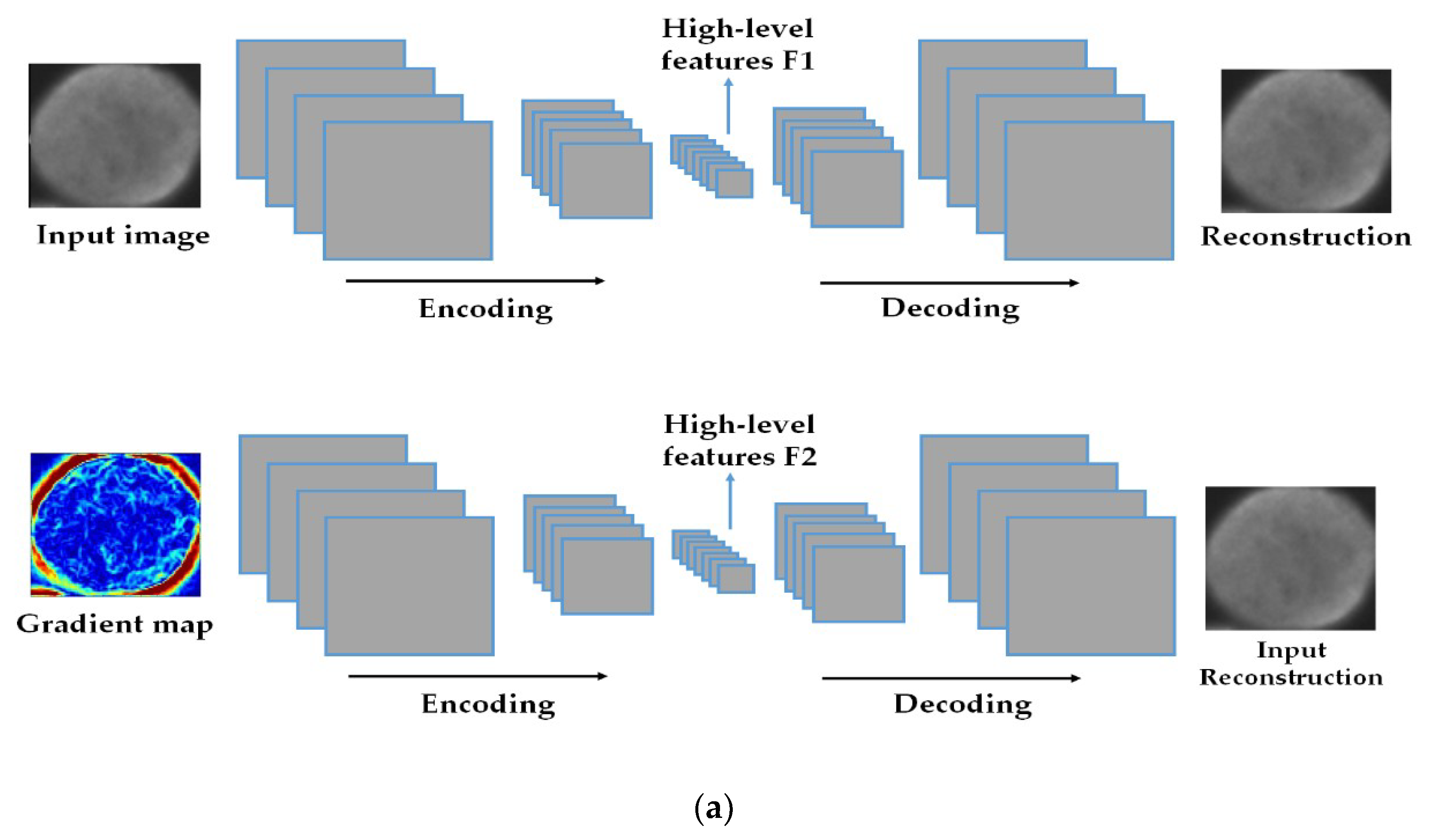
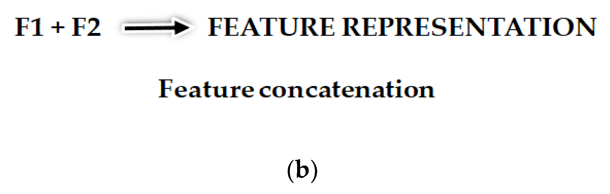
2.1. Feature Learning and Extraction using Two Levels of a Convolutional Auto-Encoder

Auto-encoders [33,34] are unsupervised learning methods that are used for the purpose of feature extraction and dimensionality reduction of the data. Neural network-based auto-encoders consist of an encoder and a decoder. The encoder takes an input signal x of dimension d, and maps it to a hidden representation y, of dimension r, using a deterministic mapping function $f$ such that:

$$\mathbf{y}=\mathrm{f}\left(\mathbf{Wx}+\mathbf{b}\right),$$

(1)

where the parameters $\mathbf{W}$ and $\mathbf{b}$ are the weights and bias matrices that are associated with the layer that takes the input x. These parameters must be learned by the encoder. The decoder then takes the output y of the encoder, computed using Equation (1), and uses the same deterministic mapping function $\mathrm{f}$ in order to provide a reconstruction z that must be of the same shape or in the same form than x, which means that the reconstructed signal z must be almost equal to the original signal x. Using Equation (1), the output z of the decoder is also given by:

$$\mathbf{z}=\mathrm{f}({\mathbf{W}}^{\prime }\mathbf{y}+{\mathbf{b}}^{\prime }),$$

(2)

where the parameters W′ and b′ are the weights and bias matrices that are associated with the decoder layer. In final, the network must learn the parameters W, W′, b, and b′, so that the reconstruction z must be close or, if possible, equal to the original input signal x. The network leans to minimize the differences between the input x and the output z.

This encoding-decoding process can be done with the use of convolutional neural networks, with what we call the DCAE. Unlike with conventional neural networks where you can fix the size of the output that you want to get, the convolutional neural networks usually incorporate in their structure the so-called pooling layers whose principal work is to retain only the maximal activations in a given region, thus, reducing the input’s spatial extent.

While using the DCAE, right after the down-sampling process is accomplished by the encoder, the decoder takes the latent representations and tries to up-sample them until we reconstruct the original size. This up-sampling process can be done by the backwards convolution, often called “deconvolution” operations, and the backwards pooling, often denoted as “unpooling” operations. The final solution of the network can be written in the form of:

$$\left(\mathbf{W},{\mathbf{W}}^{\prime },\mathbf{b},{\mathbf{b}}^{\prime }\right)=\underset{\mathbf{W},{\mathbf{W}}^{\prime },\mathbf{b},{\mathbf{b}}^{\prime }}{\mathrm{argmin}}L(\mathbf{xz}),$$

(3)

where z denotes the decoder’s output and x is the original image. Which means that the final solution of the system comprises the learned parameters W, W′, b, and b′ that minimize the most the differences between the original image and the reconstruction. The adopted cost function is a cross-entropy cost [33] described as:

$$L(\mathbf{xz})={\displaystyle \sum }_{i=1}^N[{\mathbf{x}}_i\log {\mathbf{z}}_i+\left(1-{\mathbf{x}}_i\right)\log \left(1-{\mathbf{z}}_i\right)]$$

(4)

where N represents the total number of data (total number of images used during the training process), x is the original input image, and z is the output of the decoder described in Equation (2). The network learns the parameters in Equation (3) so that the cost function described in Equation (4) is minimized. This means that the network, after down-sampling the original image, tries to reconstruct it.

In this work, we propose to use two levels of feature extraction with the DCAE. The first network will take as an input the original cellular image, and will learn to reconstruct it by using the decoding function depicted in Equation (2). The original image contains the intensity and geometric information concerning the cells. Our assumption is that the high-level features learned by this network will encapsulate the intensity and geometric information about the cellular patterns.

The second network will take the gradient magnitude of the image as the input. In every single pixel of the image, the gradients $\overrightarrow{\nabla \mathbf{I}}$, evaluated using the following equation:

$$\overrightarrow{\nabla \mathbf{I}}=\frac{\partial \mathbf{I}}{\partial x}{\mathbf{e}}_x+\frac{\partial \mathbf{I}}{\partial y}{\mathbf{e}}_y,$$

(5)

compute the rate and the direction of the changes in the intensity variation. In Equation (5), I represents the original image, and the unit vectors ${\mathbf{e}}_x$ and ${\mathbf{e}}_y$ represent the two axis of the image, the horizontal and vertical directions, along which we compute the changes in pixel level. The gradient magnitude is the magnitude of the vector $\overrightarrow{\nabla \mathbf{I}}$, whose estimation, following Equation (5), can be written as:

$$\mathbf{Gmag}(\mathbf{I})=\sqrt{{\left(\frac{\partial \mathbf{I}}{\partial x}\right)}^2+{\left(\frac{\partial \mathbf{I}}{\partial y}\right)}^2},$$

(6)

where Gmag matrix represents the gradient magnitude of the image I.

While the encoder of the first network uses the expression denoted in Equation (1) in order to compute its output, in the second network, we replace the input x by its gradient magnitude. The output vector y of the encoder from the second DCAE can be re-written as:

$$\mathbf{y}=\mathrm{f}\left(\mathbf{W}·\mathbf{Gmag}\left(\mathbf{x}\right)+\mathbf{b}\right),$$

(7)

where W and b are again the weights and bias matrices associated with the encoder. Note that the reconstruction process of the second DCAE is done in the same manner as the one of the first network. Equation (2) is used for computing the output of the decoder, and Equations (3) and (4) are used in the same manner, in order to find the best parameters that minimize the most the differences between the decoder’s output and the original cellular image. Which means that the second network takes as inputs the gradients, and, using them, try to reconstruct the original cell image.

The second assumption made here is that the gradient maps will allow the network to seize and understand the local changes in intensity level of the cellular images. The high-level features trapped in the middle of both network will be, after the networks reach convergence, extracted and concatenated in order to form our final feature vector representation.

The encoding–decoding scheme of the DCAEs requires a symmetric architecture in the two parts of the network. This means that both the encoder and decoder will have the same size and volume, and every single down-sampling layer in the encoder must have its corresponding up-sampling layer in the decoder. Because the image and its gradient map have the same size, we have used the same architecture for both DCAEs.

Their architecture is depicted in detail in

Table 1. Architecture of the DCAEs.

Layer	Filter size	#Feature Maps	Stride	Padding	Output
Input	-	-	-	-	112 × 112
Conv 1	3 × 3	32	1	1	112 × 112
Pool 1	2 × 2	32	2	0	56 × 56
Conv 2	3 × 3	64	1	1	56 × 56
Pool 2	2 × 2	64	2	0	28 × 28
Conv 3	3 × 3	128	1	1	28 × 28
Pool 3	2 × 2	128	2	0	14 × 14
Conv 4	3 × 3	256	1	1	14 × 14
Pool 4	2 × 2	256	2	0	7 × 7
Conv 5	7 × 7	512	1	1	1 × 1
Deconv 5	7 × 7	256	1	0	7 × 7
Unpool 4	2 × 2	256	2	0	14 × 14
Deconv 4	3 × 3	128	1	1	14 × 14
Unpool 3	2 × 2	128	2	0	28 × 28
Deconv 3	3 × 3	64	1	1	28 × 28
Unpool 2	2 × 2	64	2	0	56 × 56
Deconv 2	3 × 3	32	1	1	56 × 56
Unpool 1	2 × 2	32	2	0	112 × 112
Deconv 1	3 × 3	1	1	1	112 × 112

. In the table, we can clearly distinguish the down-sampling process (encoding) with the stacking of many convolutional and pooling layers. Each convolutional layer is denoted by “Conv n” in the table, with n being the nth layer that performs convolution operations on the image. The input image has a size of 112 × 112, as does the gradient map. We have avoided the use of big filters, in order to attenuate the impact of the loss of spatial information during the down-sampling process. In fact, going deeper inside the network causes a progressive loss of spatial detail, while it significantly increases the complexity of the nonlinearities provided by the cascade of the convolution operations. This finally, provides more subtle and complex features, but with a lack of accuracy in terms of reconstruction. This is the reason for why we have preferred, in order to encourage a quite fair reconstruction, the use of multiple filters of small sizes.

The idea of utilizing a cascade of small convolution filters before the pooling operations, instead of a single filter with a large spatial extent, was firstly proposed by Simonyan et al. [35], with the well-known VGG network. Most of the encoding–decoding networks in the literature, such as the ones used in the segmentation problems, for example the U-Net [36] or the SegNet [37], have adopted the VGG-like structure especially for its capability for minimizing the loss of the spatial details, which are critically necessary in case of problems that involve reconstruction. The main difference of our network with these VGG-like networks is that we have avoided the stacking of supplementary convolutional layers before the down-sampling process performed by the pooling layers. In fact, besides the fact of increasing the computational complexity of the network, we have found out that these additional layers do not improve the discrimination potentiality of the latent representations.

As we can denote in the table, every single convolutional layer uses a filter that has a fixed size of 3 × 3, except the final filter in the encoder, denoted by “Conv 5”, whose filer has a size of 7 × 7. We have used a single dimension for both the stride and the zero-padding for every single convolutional layer, in order to allow the convolution operation to keep the spatial dimension of the input volume unchanged. As we can clearly notice in the fifth column of the table denoting the output size of each operation, every convolutional layer, except Conv 5, produces an output that has the same exact size as its input. For example, Conv 1 produces an output of 112 × 112 × 32, which preserves the spatial extent of the original image.

The down-sampling mechanism is only assigned to the pooling layers. In fact, every pooling layer in the encoder has a stride of 2, and does not use any padding in such a way that the input volume is down-sampled by half after every pooling operation. The first layer of the encoder, the Conv 1 layer, has 32 different filters, and the last layer of the encoder, the Conv 5 layer, has 512 different filters. As we can remark, the output of the fourth pooling layer, Pool 4, has a size of 7 × 7 with 256 different feature maps, which gives a volume size of 7 × 7 × 256. After this step, we have used a convolution of size 7 × 7, so that the output will have one dimension. This layer has 512 different filters, which gives a 1 × 1 × 512 output. We can think of it as a vector containing 512 elements. This layer will contain the features that will be utilized subsequently as the final representation.

Just after we reach the 1 × 1 × 512 feature volume, we start the up-sampling process (decoding) with the stacking of many deconvolutional and unpooling layers. They represent the backwards operations for convolution and pooling, respectively. In the table, the deconvolutional layers are denoted as “Deconv n”, and the unpooling layers are denoted as “Unpool n”. After reaching the location of the latent representations, the decoding process starts until we reach the original size.

In the decoder, every deconvolution operation does not increase the size of the input, except for the first deconvolutional layer (Deconv 5), just like its corresponding convolutional layer in the encoder, Conv 5, which is the only convolutional layer that decreases the input size. And just like in the encoder where the down-sampling process is strictly assigned to the pooling layers, in the decoder, the up-sampling process is assigned to the unpooling layers, which also reduce the number of channels (feature maps) as we go deeper in the network until we reach the reconstruction layer that is comprised of a single channel. We can remark on the symmetry of the network in terms of size and volume.

The latent representations located in the middle of the network, in the 1 × 1 × 512 layer, precisely, will be extracted. As we use two DCAEs, we will have two vectors containing, for each one of them, 512 elements. As discussed before, the features from the two networks will be extracted and concatenated in a single vector whose size will be 1024. This means that the final feature representations, which contain the nonlinear squashing computations from the two DCAEs, will be a 1024-dimensional vector.

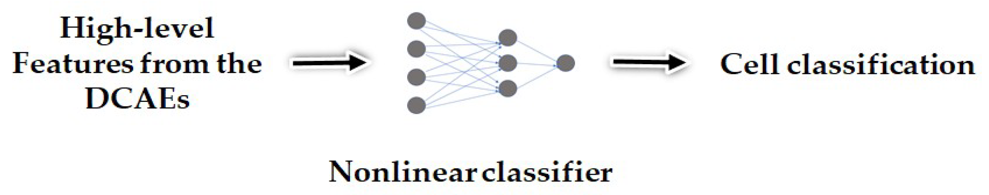
2.2. Classification Using a Nonlinear Classifier

The second part of the proposed method consists of using a shallow network for the classification of the different cell types by using the feature vectors presented in the previous section as the inputs. While this step uses a supervised learning approach, the proposed feature learning and extraction method, also presented in the previous section, utilizes a strictly unsupervised approach. As we will see in the next section, where we present the obtained results, the highly discriminatory characteristics offered by the proposed features can allow for a quite effective retrieval system with a limited number of labeled data. In fact, if we suppose that we can assign a cell type to a given unlabeled cellular image by comparing its features with the ones of the limited labeled data that we have in possession a thoroughly discriminatory feature representation is more than necessary in order to make the comparison system to be effective. This just means that the proposed features in this work can still be used in a fully unsupervised scheme in the case where labeled data are limited. The supervised step discussed in this section just serves the purpose of evaluating the discrimination potentiality of the proposed features over the publicly available labeled datasets.

Once we have our feature vectors, we can construct our artificial neural network-based classifier. The network has an input layer containing 1024 neurons, according the length of our feature vectors. We have tested different architectures and chosen the best one by cross-validating all the different models. The details on the selected architecture are discussed in the next section, and the network learns by back-propagating the error [38] from the classification layer to the input layer.

3. Results

In order to evaluate the proposed method, we have used two of the most popular publicly available datasets for the HEp-2 cell classification, the SNPHEp-2 and the ICPR 2016 datasets. Because these datasets have different levels of heterogeneity, every method gives different results when they are applied to them, which obliges us to present the results separately. All of the experiments were conducted with MATLAB (9.4 (R2018a), Natick, MA, USA), and performed on a computer with a Core i7 3.40 GHz processor and 8 GB of RAM. A GPU implementation was used with a NVIDIA GeForce GTX 1080 Ti with 11,264 MB of memory, which accelerates the training time.

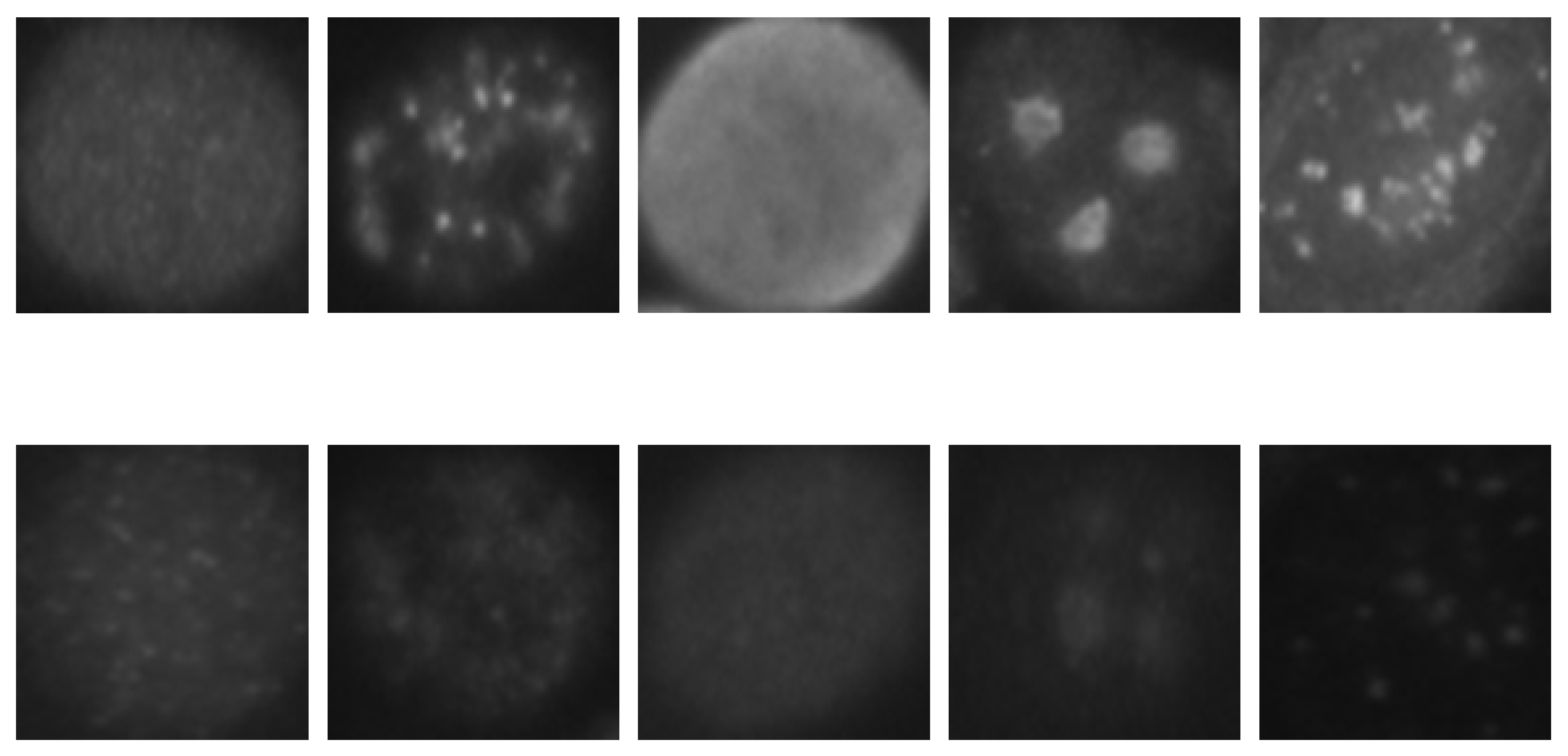
3.1. SNPHEp-2 Dataset

The SNPHEp-2 dataset was obtained between January and February 2012 at the Sullivan Nicolaides Pathology laboratory at Australia. The dataset has five patterns: the centromere, the coarse speckled, the fine speckled, the homogeneous, and the nucleolar types. The images depicted in Figure 1 were obtained from this dataset. It is composed of 40 different specimens, and every single specimen image was captured using a monochrome camera, which was fitted on a microscope with a plan-Apochromat 20×/0.8 objective lenses and an LED illumination source. In order to automatically extract the image masks, which specifically delimits the cells body, the DAPI image channel was utilized.

There are 1884 cellular images in the dataset, all of them extracted from the 40 different specimen images. Different specimen were used for constructing the training and testing image sets, and both sets were created in such a way that they cannot contain images from the same specimen. From the 40 specimens, 20 were used for the training sets and the remaining 20 were used for the testing sets. In total, there are 905 and 979 cell images for the training and testing sets, respectively. Each set (training and testing) contains five-fold validation splits of randomly selected images. In each set, the different splits are used for cross validating the different models, each split containing 450 images approximatively. The SNPHEp-2 dataset was presented by Wiliem et al. [5], and it can be downloaded freely at http://staff.itee.uq.edu.au/lovell/snphep2/.

The original images have different sizes, with average resolution of 90 × 90 pixels. The images were all resized to 112 × 112, in order to fit them into our proposed architecture. We begin our scheme by feeding the images to the two DCAEs, in order to extract the features. As explained in the previous section, two levels of feature extraction are used in our work: the first DCAE takes the original image and learns the parameters so that the image is reconstructed, and the second DCAE takes the gradient magnitude as the input and learns to reproduce the original cellular image.

In Figure 4, we can see the different images showing the projections of the final vectors constructed by merging the latent representations learned by the two DCAEs. The projections were obtained using the principal component analysis [39]. PC₁ and PC₂ denote the first and second principal component axis, respectively. For all the figures, “Homo”, “Coarse”, “Fine”, “Nucl”, and “Centro” denote the homogeneous, the coarse speckled, the fine speckled, the nucleolar, and the centromere types, respectively. In Figure 4a, we have the features constructed by using the first convolutional layers of the two networks. We called them the low-level features, because they are located right at the beginning of the networks where no meaningful features were yet learned. We can notice how the different types of the cells are mixed together. The fine speckled cells (shown in magenta color) exhibited very different patterns, as we can also remark in Figure 1, explaining why some of them were clustered away from the other types. In Figure 4b, we show the features that were learned by the third convolutional layers of the two DCAEs. We can see how both networks have already learned some distinguishable features from the data, as the different clusters started to become clearer, compared to the projections shown in Figure 4a.

In Figure 4c, we show the high-level features that were constructed by using the latent representations from the middle of the networks, the fifth convolutional layers. We can see how discriminative these features are. A part of the coarse speckled and the nucleolar cells are still clustered together, but, in a general view, we can clearly recognize five distinctive clusters from the images. The next step will consist of feeding those features, the ones shown in Figure 4c, to a nonlinear classifier that can automatically learn to discriminate them. As discussed previously, the feature vectors have a dimension of 1024. We have trained a neural network for the final classification step. The network has an input layer containing 1024 neurons, one single hidden layer containing 100 neurons, and the final layer has five neurons according to the five cell types of the dataset. The hidden layer uses the hyperbolic tangent as activation function and the last layer uses the softmax function [33] in order to output the class probabilities.

The classification results are partially shown in Figure 5, where we present the receiver operating characteristic (ROC) curves for the classification of each one of the cell types. For each cell type, the ROC curves were evaluated by considering the concerned cell type as a positive class, and all the remaining types were considered as the negative class. For example, the ROC curve of the homogeneous cells was computed by considering the homogeneous images as being from the positive class, and all the remaining cells, the four other types, as being from the negative class. The curves show how the network manages to recognize every single cell type.

We can see in Figure 5, that the centromere cells are really well recognized by the classifier, and their ROC curve, drawn using the black color, showing the best classification accuracy in the figure. This is not surprising at all if we take a look at the features shown in Figure 4c. In fact, we can see in the figure that the features from the centromere cells, shown in black dots, are clustered in a quite distinctive subspace, demonstrating that the centromere cell images exhibit particularly singular patterns. The homogeneous and fine speckled cells also occupy distinctive subspaces in Figure 4c. We can see that their ROC curves, shown in red (Homo) and magenta (Fine), are similar, which means that network manages to recognize them in a quite similar way. This may come from the fact that their patterns exhibit similar circular shapes, as we can notice in the images depicted in Figure 1. In fact, in Figure 1, the homogeneous and the fine specked images are the ones that exhibit strong circular shades in their intensity variation.

The nucleolar and the coarse speckled cells, shown in blue (Coarse) and green (Nucl) in Figure 4c, also exhibit quite similar patterns and they are relatively clustered in the same subspace. As a consequence, the classifier did have some difficulties in discriminating them properly. They present the least accurate ROC curves among all the five cell types.

In Figure 6, we show the confusion matrix of the results obtained for the classification. We recall that the testing set comprises 979 cell images. As for the ROC curves, we can notice that all the centromere cells in the testing set are well-classified by the network, giving an accuracy of 100% for this cell type. The classifier achieves 98.17% of accuracy for the discrimination of the homogeneous cells, and we can remark that a few of them, only 1.83%, are misclassified as being fine speckled. The same thing occurs for the fine speckled cell images, as 97.86% of them were well-classified, and only 2.14% of the images were wrongly classified as being homogeneous.

The least accurate performance comes with the discrimination of the coarse speckled and the nucleolar cell images. As the position of the projection subspaces occupied by their features can suggest in Figure 4c, and also as their ROC curves suggest, we can notice that the classifier achieves 95.10% of accuracy for the coarse speckled, and 94.77% for the nucleolar. This gives a total accuracy of 97.18% for the overall classification of the cells. As we will see later, most of the hand-crafted features do not surpass the 85% and the state-of-the-art deep learning-based methods stagnate around 95% of accuracy for this particular dataset.

An interesting comparison is made in Figure 7, where we show the results obtained using the features learned by the two DCAEs, but separately. In Figure 7a, we have the results using the features from the DCAE that takes as inputs only the original cellular images. The architecture of the classifier was set to be 512-50-10-5, which means that we have used two hidden layers, the first one having 50 neurons and the second one, 10 neurons. Here, the input layer has 512 neurons because one single DCAE outputs a feature vector of 512 dimensions. As we can see in Figure 7a, by computing the mean accuracy of all the classes, the network achieves a total accuracy of 71.77%.

Two important remarks about these results should be mentioned. The first one is that the features learned by the DCAE from only the original images increase the confusion between the homogeneous and the fine speckled cell images. As we can see in Figure 7a, 17.32% of the homogeneous cells were misclassified as fine speckled, and even 19.63% of the fine speckled were misclassified as homogeneous. The second remark is that the nucleolar cells are almost equivalently mixed with the coarse speckled and the centromere. This comes from the similar appearance of these three types of cells in their shapes and intensities. However, if we take a look at the results depicted in Figure 7b, where the features were learned using the gradients of the images, we can see that the confusion between these three cells radically decreases. In fact, the local changes in intensity captured by the gradients allow the features to well distinguish these cells. The hybrid feature extraction method proposed in this work allows to capture, at the same time, the features that help to recognize the cells in their global shape and also the features that help the recognition using the local changes in intensity. Which helps to efficiently discriminate the images that are globally similar but locally distinguishable (different). The classifier achieves a total accuracy of 86% into the results shown in Figure 7b. We can remark that the gradients of the cells bring more discriminant features. The confusion between the centromere and the coarse speckled is also radically attenuated.

In

Table 2. Comparative study for the SNPHEp-2 dataset.

Method	Authors	Description	Accuracy
Hand-crafted features	Nigam et al. [31]	Texture features + SVM	80.90%
	Wiliem et al. [5]	DCT features + SIFT + SVM	82.50%
	Nosaka et el. [6]	LPB + SVM	85.71%
Deep Learning	Gao et al. [22]	5 layers CNN	86.20%
	Bayramoglu et al. [29]	4 layers CNN	88.37%
	Li et al. [23]	Deep Residual Inception Model	95.61%
	Lei et al. [27]	Cross-modal transfer learning	95.99%
	Shen et al. [28]	Use of a Deep-Cross Residual Module	96.26%
	Proposed method	Double DCAEs feature extraction + ANN 1	97.18%

¹ ANN stands for artificial neural network.

, we show the results of the different methods in the literature. We separate the hand-crafted features based methods with the ones that utilize deep learning. The texture features [31], the hybrid feature representation from the DCT and the SIFT descriptors [5], and also the LPB descriptors [6] achieve, respectively, 80.90%, 82.50%, and 85.71%.

The first deep learning based method [22] was proposed for the ICPR 2012 dataset, which contains less images compared to the SNPHEp-2 dataset, but also is far less heterogeneous. That is why the method performs poorly on this dataset, which contains more diversified data from many more specimens, accomplishing an accuracy of 86.20%. Bayramoglu et al. [29] have utilized a quite similar architecture with the network, as proposed in [22], but their method uses a consequent data augmentation, achieving 88.37%. The state-of-the-art deep learning based methods in [23,27], and [28] stagnate at 95.61%, 95.99%, and 96.26%, respectively, for this dataset.

3.2. ICPR 2016 Dataset

The first ICPR HEp-2 classification contest had proposed the ICPR 2012 dataset, which was not really heterogeneous. Since 2013, they have provided more heterogeneous datasets, like the one used during the 2016 edition, the ICPR 2016 dataset [32]. The images were taken with an acquisition unit consisting of the fluorescence microscope, coupled with a 50 W mercury vapor lamp and a digital camera. The images are made from 83 different specimens, which significantly reinforces the intra-class heterogeneity.

The dataset contains six different cellular types: the homogeneous (2494 images from 16 different specimens), the speckled (2831 images, 16 specimens), the nucleolar (2598 images, 16 specimens), the centromere (2741 images, 16 specimens), the nuclear membrane (2208 images, 15 specimens), and the Golgi (724 images, only four specimens). The dataset contains in total, 13,596 images, and it can be downloaded at http://mivia.unisa.it/datasets/biomedical-image-datasets/hep2-image-dataset/. We show some sample images from this dataset in Figure 8.

The size of the images from this dataset roughly varies around 95 × 95 pixels and, just like with the previous dataset, we have resized them to 112 × 112 before giving them to the DCAEs. We started by extracting the features using the two-level DCAE, and then the extracted features were given to a neural network for the classification step. Among the 13,596 images, 80% were utilized for training both the DCAEs and the artificial neural networks (ANNs), and the remaining 20% were used for testing the models.

We show two results for this dataset. The first ones are shown in the confusion matrix depicted in Figure 9. In the figure, “Homo”, “Speck”, “Nucl”, “Centro”, “NucM”, and “Golgi” denote, respectively, the homogeneous, speckled, nucleolar, centromere, nuclear membrane, and Golgi cells. These results were obtained by using a network with the same exact architecture compared to the one used for the previous dataset. This means that the input layer contains 1024 neurons with one single hidden layer containing 100 neurons. The final layer has six neurons in this case, because we have six different classes. In Figure 9, we can see that all of the Golgi cells were recognized by the classifier. The speckled cells were slightly confused with the homogeneous cells, but the accuracy for each one of the classes remained at a high level. The total accuracy was about 97.38%.

When we tried to use a much deeper architecture for the ANN classifier, the accuracy increased. While the best results for the previous dataset were found with this architecture, we found that the best results for this dataset were with a 1024-250-20-6 architecture. The input layer took the 1024 elements of the feature vectors, two hidden layers were used, the first one had 250 neurons and the second one had 20 neurons, and the final layer comprised the six neurons corresponding to the six different cell types for classification. The results are shown in detail in Figure 10.

We can remark in the results shown in Figure 10 that the network slightly decreased the confusion between the homogeneous and the speckled cells, and also between the centromere and the nucleolar. All of the Golgi cells were still well-recognized by the network and, moreover, any confusion between the nuclear membrane and the speckled cells disappeared, and the total accuracy of the network was 98.66%.

The comparison study for this dataset is shown in

Table 3. Comparative study for the ICPR 2016 dataset.

Method	Authors	Description	Accuracy
Hand-crafted features	Nigam et al. [31]	Texture features + SVM	71.63%
	Wiliem et al. [5]	DCT features + SIFT + SVM	74.91%
	Nosaka et el. [6]	LPB + SVM	79.44%
Deep Learning	Gao et al. [22]	5 layers CNN	96.76%
	This work	Double DCAE feature extraction + ANN-1024-100-6	97.38%
	Xi et al. [29]	VGG-like network	98.26%
	Li et al. [23]	Deep Residual Inception Model	98.37%
	Lei et al. [27]	Cross-modal transfer learning	98.42%
	Shen et al. [28]	Use of a Deep-Cross Residual Module	98.62%
	This work	Double DCAE feature extraction + ANN-1024-200-20-6	98.66%

. For all the methods in the table, we used the same training–testing split, in order to minimize the splitting-related biases, and to make the comparative study more reliable. The heterogeneity of this dataset poses certain problems for the hand-crafted feature-based methods. Their accuracy really decreases greatly when we compare the results in Table 3 with the ones depicted in Table 2 for the previous dataset. The reason for is that many, if not all, of these methods were proposed when the datasets for the HEp-2 cells were not diversified enough.

In contrast, all of the deep learning based methods were specifically proposed for this dataset, which is why all of them reached outstanding results here. We can clearly see in Table 3 that our proposed method performed as well as the state-of-the-art deep learning methods. Moreover, when the classification step was performed with a much deeper network, our method relatively surpassed the other methods. We recall that our method is mainly based on a strictly unsupervised feature learning method, which can help in the case where labeling the images can be an arduous work.

4. Conclusions

HEp-2 cell classification is one of the most important steps for automated diagnosis of autoimmune diseases. We have proposed a classification method that, unlike most of the state-of-the-art methods, uses a deep learning-based feature extraction framework in an unsupervised way. We have proposed the use of two deep convolutional autoencoders. The first network takes the original cellular images as the inputs, and learns to reconstruct them in order to capture the features that are related to the global shape of the cells, and the second network takes the gradients of the images as inputs, and learns to reconstruct the original images in order to encode the local changes in the intensity of the images provided by their gradient maps.

Then, a final feature vector is constructed by combining the latent representations extracted from the two networks, giving a highly discriminative feature representation. The high discriminability of the proposed features was tested on two of the most popular HEp-2 cell classification datasets, the SNPHEp-2 and ICPR 2016 datasets. The results show that the proposed features manage to capture the distinctive characteristics of the different cell types while performing at least as well as the actual deep learning-based state-of-the-art methods.

References

1. Rigon, A.; Soda, P.; Zennaro, D.; Iannello, G.; Afeltra, A. Indirect immunofluorescence in autoimmune diseases: Assessment of digital images for diagnostic purpose. Cytom. B Clin. Cytom. 2007, 72, 472–477. [Google Scholar] [CrossRef] [Green Version]
2. Foggia, P.; Percannella, G.; Soda, P.; Vento, M. Benchmarking hep-2 cells classification methods. IEEE Trans. Med. Imaging 2013, 32, 1878–1889. [Google Scholar] [CrossRef] [PubMed]
3. Foggia, P.; Percannella, G.; Saggese, A.; Vento, M. Pattern recognition in stained hep-2 cells: Where are we now? Pattern Recognit. 2014, 47, 2305–2314. [Google Scholar] [CrossRef]
4. Cataldo, S.D.; Bottino, A.; Ficarra, E.; Macii, E. Applying textural features to the classification of HEp-2 cell patterns in IIF images. In Proceedings of the 21st International Conference on Pattern Recognition (ICPR2012), Tsukuba, Japan, 11–15 November 2012; pp. 689–694. [Google Scholar]
5. Wiliem, A.; Wong, Y.; Sanderson, C.; Hobson, P.; Chen, S.; Lovell, B.C. Classification of human epithelial type 2 cell indirect immunofluorescence images via codebook based descriptors. In Proceedings of the 2013 IEEE Workshop on Applications of Computer Vision (WACV), Tampa, FL, USA, 15–17 January 2013; pp. 95–102. [Google Scholar] [CrossRef]
6. Nosaka, R.; Fukui, K. Hep-2 cell classification using rotation invariant co-occurrence among local binary patterns. Pattern Recognit. 2014, 47, 2428–2436. [Google Scholar] [CrossRef]
7. Huang, Y.C.; Hsieh, T.Y.; Chang, C.Y.; Cheng, W.T.; Lin, Y.C.; Huang, Y.L. HEp-2 cell images classification based on textural and statistic features using self-organizing map. In Proceedings of the 4th Asian Conference on Intelligent Information and Database Systems, Part II, Kaohsiung, Taiwan, 19–21 March 2012; pp. 529–538. [Google Scholar]
8. Thibault, G.; Angulo, J.; Meyer, F. Advanced statistical matrices for texture characterization: Application to cell classification. IEEE Trans. Biomed. Eng. 2014, 61, 630–637. [Google Scholar] [CrossRef] [PubMed]
9. Wiliem, A.; Sanderson, C.; Wong, Y.; Hobson, P.; Minchin, R.F.; Lovell, B.C. Automatic classification of human epithelial type 2 cell indirect immunofluorescence images using cell pyramid matching. Pattern Recognit. 2014, 47, 2315–2324. [Google Scholar] [CrossRef]
10. Xu, X.; Lin, F.; Ng, C.; Leong, K.P. Automated classification for HEp-2 cells based on linear local distance coding framework. J. Image Video Proc. 2015, 2015, 1–13. [Google Scholar] [CrossRef]
11. Cataldo, S.D.; Bottino, A.; Islam, I.U.; Vieira, T.F.; Ficarra, E. Subclass discriminant analysis of morphological and textural features for hep-2 staining pattern classification. Pattern Recognit. 2014, 47, 2389–2399. [Google Scholar] [CrossRef]
12. Bianconi, F.; Fernández, A.; Mancini, A. Assessment of rotation-invariant texture classification through Gabor filters and discrete Fourier transform. In Proceedings of the 20th International Congress on Graphical Engineering (XX INGEGRAF), Valencia, Spain, 4–6 June 2008. [Google Scholar]
13. Ojala, T.; Pietikainen, M.; Maenpaa, T. Multiresolution gray-scale and rotation invariant texture classification with local binary patterns. IEEE Trans. Pattern Anal. Mach. Intell. 2002, 24, 971–987. [Google Scholar] [CrossRef] [Green Version]
14. Nosaka, R.; Ohkawa, Y.; Fukui, K. Feature extraction based on co-occurrence of adjacent local binary patterns. In Proceedings of the 5th Pacific Rim Symposium on Advances in Image and Video Technology, Part II, Gwangju, Korea, 20–23 November 2012; pp. 82–91. [Google Scholar]
15. Guo, Z.; Zhang, L.; Zhang, D. A completed modeling of local binary pattern operator for texture classification. IEEE Trans. Image Process. 2010, 19, 1657–1663. [Google Scholar] [CrossRef]
16. Theodorakopoulos, I.; Kastaniotis, D.; Economou, G.; Fotopoulos, S. Hep-2cells classification via sparse representation of textural features fused into dissimilarity space. Pattern Recognit. 2014, 47, 2367–2378. [Google Scholar] [CrossRef]
17. Ponomarev, G.V.; Arlazarov, V.L.; Gelfand, M.S.; Kazanov, M.D. ANA hep-2 cells image classification using number, size, shape and localization of targeted cell regions. Pattern Recognit. 2014, 47, 2360–2366. [Google Scholar] [CrossRef]
18. Shen, L.; Lin, J.; Wu, S.; Yu, S. Hep-2 image classification using intensity order pooling based features and bag of words. Pattern Recognit. 2014, 47, 2419–2427. [Google Scholar] [CrossRef]
19. LeCun, Y.; Bengio, Y.; Hinton, G. Deep learning. Nature 2015, 521, 436–444. [Google Scholar] [CrossRef] [PubMed]
20. LeCun, Y.; Huang, F.J.; Bottou, L. Learning methods for generic object recognition with invariance to pose and lighting. In Proceedings of the 2004 IEEE Computer Society Conference on Computer Vision and Pattern Recognition (CVPR’04), Washington, DC, USA, 27 June–2 July 2004. [Google Scholar]
21. Krizhevsky, A.; Sutskever, I.; Hinton, G.E. ImageNet classification with deep convolutional neural networks. In Proceedings of the 25th International Conference on Neural Information Processing Systems (NIPS’12), Lake Tahoe, NV, USA, 3–6 December 2012; pp. 1097–1105. [Google Scholar]
22. Gao, Z.; Wang, L.; Zhou, L.; Zhang, J. Hep-2 cell image classification with deep convolutional neural networks. IEEE J. Biomed. Health Inf. 2017, 21, 416–428. [Google Scholar] [CrossRef] [PubMed]
23. Li, Y.; Shen, L. A deep residual inception network for HEp-2 cell classification. In Proceedings of the 3rd International Workshop on Deep Learning in Medical Image Analysis (DLMIA 2017), Québec City, QC, Canada, 14 September 2017; pp. 12–20. [Google Scholar]
24. He, K.; Zhang, X.; Ren, S.; Sun, J. Deep residual learning for image recognition. In Proceedings of the 2016 IEEE Conference on Computer Vision and Pattern Recognition, Las Vegas, NV, USA, 27–30 June 2016; pp. 770–778. [Google Scholar]
25. Szegedy, C.; Liu, W.; Jia, Y.; Sermanet, P. Going deeper with convolutions. In Proceedings of the 2015 IEEE Conference on Computer Vision and Pattern Recognition, Boston, MA, USA, 7–12 June 2015; pp. 1–9. [Google Scholar]
26. Phan, H.T.H.; Kumar, A.; Kim, J.; Feng, D. Transfer learning of a convolutional neural network for HEp-2 cell image classification. In Proceedings of the 2016 IEEE 13th International Symposium on Biomedical Imaging (ISBI), Prague, Czech Republic, 13–16 June 2016; pp. 1208–1211. [Google Scholar]
27. Lei, H.; Han, T.; Zhou, F.; Yu, Z.; Qin, J.; Elazab, A.; Lei, B. A deeply supervised residual network for HEp-2 cell classification via cross-modal transfer learning. Pattern Recognit. 2018, 79, 290–302. [Google Scholar] [CrossRef]
28. Shen, L.; Jia, X.; Li, Y. Deep cross residual network for HEp-2 cell staining pattern classification. Pattern Recognit. 2018, 82, 68–78. [Google Scholar] [CrossRef]
29. Bayramoglu, N.; Kannala, J.; Heikkilä, J. Human epithelial type 2 cell classification with convolutional neural networks. In Proceedings of the IEEE 15th International Conference on Bioinformatics and Bioengineering (BIBE), Belgrade, Serbia, 2–4 November 2015; pp. 1–6. [Google Scholar]
30. Xi, J.; Linlin, S.; Xiande, Z.; Shiqi, Y. Deep convolutional neural network based HEp-2 cell classification. In Proceedings of the 2016 23rd International Conference on Pattern Recognition (ICPR), Cancun, Mexico, 4–8 December 2016; pp. 77–80. [Google Scholar]
31. Nigam, I.; Agrawal, S.; Singh, R.; Vatsa, M. Revisiting HEp-2 cell classification. IEEE Access 2015, 3, 3102–3113. [Google Scholar] [CrossRef]
32. Lovell, B.C.; Percannella, G.; Saggese, A.; Vento, M.; Wiliem, A. International contest on pattern recognition techniques for indirect immunofluorescence images analysis. In Proceedings of the 2016 23rd International Conference on Pattern Recognition (ICPR), Cancun, Mexico, 4–8 December 2016; pp. 74–76. [Google Scholar]
33. Bengio, Y. Learning deep architecture for AI. Foundat. Trends Mach. Learn. 2009, 2, 1–127. [Google Scholar] [CrossRef]
34. Hinton, G.E.; Salakhutdinov, R.R. Reducing the dimensionality of the data with neural networks. Science 2006, 313, 504–507. [Google Scholar] [CrossRef]
35. Simonyan, K.; Zisserman, A. A very deep convolutional networks for large-scale image recognition. In Proceedings of the 2015 International Conference on Learning Representation (ICLR15), San Diego, CA, USA, 7–9 May 2015. [Google Scholar]
36. Ronneberger, O.; Fischer, P.; Brox, T. U-Net: Convolutional networks for biomedical image segmentation. In Proceedings of the 18th International Conference on Medical Image Computing and Computer-Assisted Intervention (MICAAI 2015), Munich, Germany, 5–9 October 2015; pp. 234–241. [Google Scholar]
37. Badrinarayana, V.; Kendall, A.; Cipolla, R. SegNet: A deep convolutional encoder-decoder architecture for Image Segmentation. IEEE Trans. Pattern Anal. Mach. Intell. 2017, 39, 2481–2495. [Google Scholar] [CrossRef] [PubMed]
38. Rumelhart, D.E.; Hinton, G.E.; Williams, R.J. Learning representations by back-propagating errors. Nature 1986, 323, 533–536. [Google Scholar] [CrossRef]
39. Hotelling, H. Analysis of a complex of statistical variables into principal components. J. Educ. Psychol. 1933, 24, 417–441. [Google Scholar] [CrossRef]
Figure 1. HEp-2 cell images from one of the used datasets. In the first row, we have the positive intensity images while the second row depicts the intermediate intensity images. For both rows we have, from left to right, homogeneous, coarse speckled, fine speckled, nucleolar, and centromere cells.
Electronics 08 00020 g001
Figure 2. The schematic representation of the proposed method. In (a), we have a two-level deep-learning feature extraction by using two deep convolutional auto-encoders (DCAEs): the first DCAE takes the original image as an input and learns to reproduce it while the second one takes the image gradients and learns to reproduce the original cellular image. In (b), the latent representations from the two DCAEs are extracted and concatenated in one single vector to form the final feature representation.
Electronics 08 00020 g002aElectronics 08 00020 g002b
Figure 3. The high-level features are used as the inputs of a nonlinear classifier for the cell classification step.
Electronics 08 00020 g003
Figure 4. Visualization of the features learned by the DCAEs. In (a), we have the low-level features extracted from the first convolutional layer, as denoted by Conv 1 in Table 1. In (b), we have the middle-level features from the Conv 3 layer, and in (c), we can see the high-level features from the Conv 5 layer.
Electronics 08 00020 g004
Figure 5. ROC curves for the classification of every single cell type.
Electronics 08 00020 g005
Figure 6. Confusion matrix of the results using the proposed method over the testing set. The total accuracy of the classifier is 97.18%.
Electronics 08 00020 g006
Figure 7. Confusion matrix of the classification results over the test set. In (a), the features were learned with only the original cell images and in (b), the features were obtained by using only the image gradients.
Electronics 08 00020 g007
Figure 8. Examples of HEp-2 cell images from the ICPR 2016 dataset. In (af), we have, respectively, the homogeneous, the speckled, the nucleolar, the centromere, the nuclear membrane, and the Golgi.
Electronics 08 00020 g008
Figure 9. Confusion matrix of the classification for the ICPR 2016 dataset using a 1024-100-6 network architecture. The total accuracy is 97.38%.
Electronics 08 00020 g009
Figure 10. Confusion matrix of the classification for the ICPR 2016 dataset using a 1024-250-20-6 network architecture. The total accuracy is 98.66%.
Electronics 08 00020 g010