BP Neural Network-Based Adaptive Phase-Locked Loop for Impedance Measurement with Dynamic Operating Conditions

Abstract

With the development of modern power systems, impedance measurement has become a key approach for stability assessment of power-electronic-dominated grids. In particular, frequency-sweep–based impedance measurement is widely adopted due to its effectiveness in characterizing system dynamics. However, owing to the limited adaptability of conventional phase-locked loop (PLL), grid-following (GFL) converters encounter significant challenges in maintaining stable operation during frequency-sweep signal injection, especially under non-power-frequency excitation and grid disturbances. To address these issues, this paper proposes an adaptive PLL scheme based on a backpropagation (BP) neural network. This scheme fully leverages the nonlinear mapping and adaptive learning capabilities of the BP neural network, which significantly enhances the robustness and stability adaptability of the synchronization component against small disturbances during the impedance measurement process. A hybrid strategy combining offline parameter tuning and online adaptive adjustment is adopted to improve reliability under varying operating conditions. Comprehensive simulation studies and hardware-in-the-loop (HIL) experimental results verify the effectiveness of the proposed method in improving stability and impedance measurement accuracy in frequency-sweep–based applications.

1. Introduction

With the development of distributed generation technology, the traditional power generation mode has gradually shifted towards distributed generation [1]. Modern power systems are evolving toward highly dynamic and converter-dominated networks. Under such conditions, system stability is no longer solely determined by network parameters but is strongly influenced by the interaction between converters and the grid. Impedance-based analysis has therefore become a fundamental tool for stability assessment, oscillation diagnosis, and interaction mechanism identification in modern power systems.

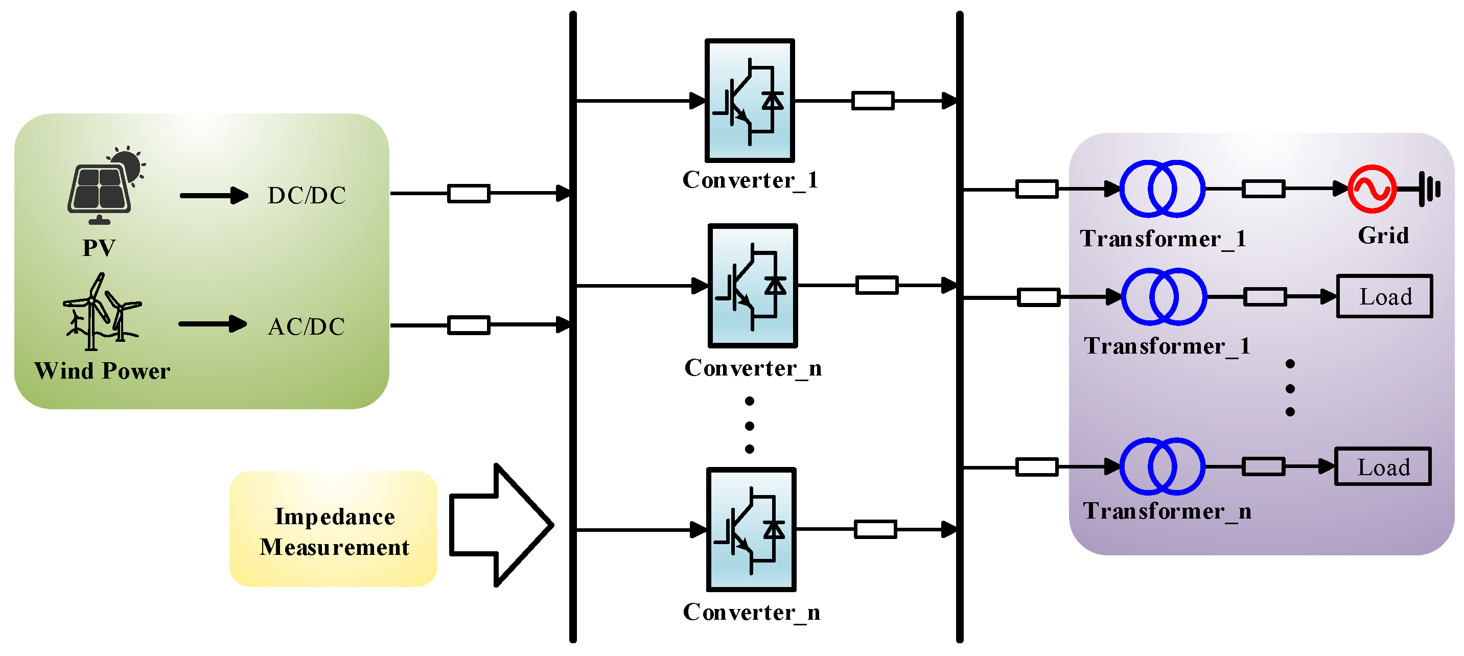
Among various impedance identification techniques, frequency-sweep–based online impedance measurement has been widely adopted due to its capability of capturing broadband dynamic characteristics without requiring access to internal controller information [2]. By injecting small-signal perturbations at multiple frequencies and analyzing the system response, frequency-sweep methods enable accurate impedance characterization over a wide frequency range. Impedance measurement is the technical foundation for key scenarios such as oscillation prediction, islanding detection, and weak-characteristic fault diagnosis, and its measurement accuracy directly determines the reliability of power grid operating state assessment [3]. As shown in Figure 1, converters numbered from Converter_1 to Converter_n are all connected to renewable energy sources and can be reused for impedance measurement while normally outputting power frequency current [4].

However, frequency-sweep impedance measurement imposes unique and stringent requirements on GFL converters, which are commonly equipped with a PLL for grid synchronization. Unlike conventional steady-state grid-connected operation, frequency-sweep measurement continuously injects non-power-frequency disturbances with varying frequencies and amplitudes, causing the converter to operate under persistent multi-frequency excitation. Under such conditions, the fundamental assumptions underlying conventional synchronous reference frame PLL (SRF-PLL), namely, near-sinusoidal voltage, are no longer valid. Under the above conditions, frequency sweep injection signals and power-grid disturbances will inevitably be coupled through the PLL and the internal control links of the converter, thereby causing phase estimation errors, dynamic performance degradation, and distortion of impedance measurement results. In extreme cases, the frequency sweep process may even lead to phase-locking loss of synchronization or system instability [1]. The degradation of PLL performance will directly affect the accuracy and reliability of impedance measurement. Therefore, the PLL has become one of the important bottlenecks limiting the engineering application of frequency sweep impedance measurement.

Existing PLL enhancement techniques, such as alternative PLL structures [5], or additional filtering [6,7], can partially improve robustness under specific disturbances. However, these approaches are typically designed based on fixed analytical models and tuned for predefined operating conditions. During frequency-sweep impedance measurement, the operating point, disturbance frequency, and signal coupling characteristics vary continuously, making it difficult for conventional model-based PLL designs to maintain optimal synchronization performance across the entire sweep range. Consequently, a PLL with strong adaptability to multi-frequency, non-stationary excitation is highly desirable for frequency-sweep applications.

At present, existing studies have applied AI algorithms to GFL control, which is conducive to improving stability [8,9]. To address the challenge, this paper proposes an adaptive PLL scheme based on a BP neural network, specifically targeting frequency-sweep impedance measurement scenarios. By leveraging the nonlinear mapping and adaptive learning capability of the BP neural network, the proposed PLL can dynamically adjust its parameters in response to varying sweep frequencies and grid conditions, thereby maintaining accurate phase tracking and robust synchronization. A hybrid strategy combining offline parameter tuning and online adaptive adjustment is adopted to ensure both reliability and real-time adaptability during the sweep process.

The remainder of this paper is organized as follows. Section 2 introduces the application scenarios and system topology of GFL converters for frequency-sweep impedance measurement and presents the dq-frame impedance modeling framework. Section 3 details the proposed BP-neural-network-based adaptive PLL and its implementation. Section 4 provides stability analysis and qualitative insights into the impedance behavior under frequency-sweep excitation. Section 5 presents simulation and HIL experimental results to validate the proposed method. Finally, Section 6 concludes the paper and discusses future research directions.

2. System Configuration and Scenarios

In frequency sweep-based impedance measurement, GFL converters are widely employed as disturbance signal generators. This paper takes a single GFL with a DC voltage outer-loop control as the research object. By improving the phase-locked loop PLL of the GFL, its adaptability to various impedance measurement scenarios is enhanced.

2.1. System Configuration

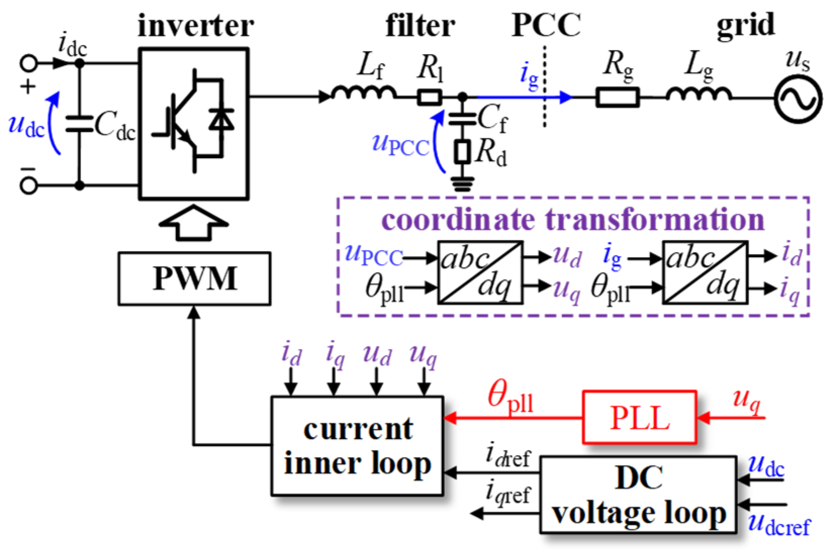
The GFL studied in this paper operates in the impedance measurement scenario and serves as a reused device in the system. The system block diagram of a GFL connected to a weak grid is shown in Figure 2. The system circuit part consists of an inverter bridge, a filter, and a weak grid. The control part includes a PLL, a DC voltage loop, and a current inner loop. In this system, Subscripts d and q denote the d-axis and q-axis components, respectively. u_dc denotes the DC-side capacitor voltage. L_f is the machine-side filter inductor. C_f is the filter capacitor, and R_d is the damping resistor. L_g is the grid-side inductance, and R_g is the grid-side resistance. Since the grid impedance is dominated by inductive characteristics, R_g is assumed to be 0 for the sake of simplifying the analysis. i_g is the grid-connected current. u_s denotes the ideal voltage source.

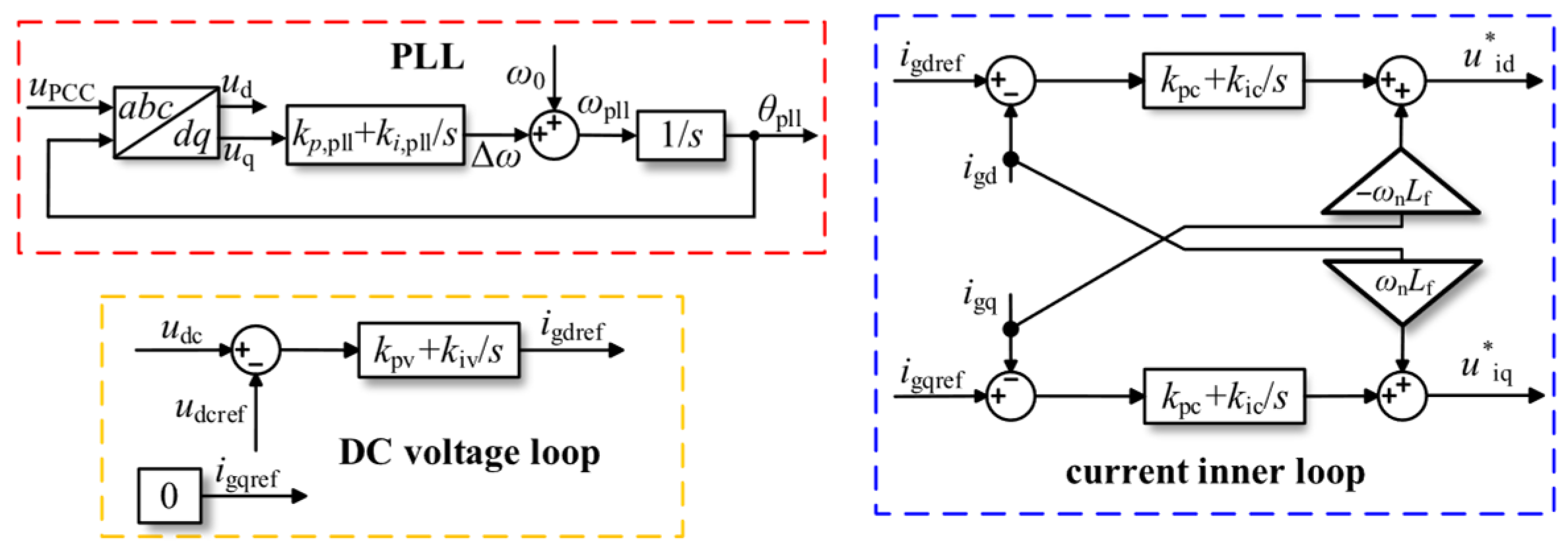
Figure 3 shows the basic control of a GFL, including a PLL, a DC voltage loop, and a current inner loop. The PLL collects the point of common coupling (PCC) voltage and outputs the reference phase angle of the sinusoidal signal. The DC voltage loop incorporates a proportional-integral (PI) regulator, which outputs the d-axis current reference value. The current inner loop incorporates a PI regulator and a dq-axis decoupling control unit. The output of the current loop serves as the reference value for the bridge arm voltage.

The basic parameters of the model in this paper are shown in

Table 1. Basic system parameters.

Symbol	Parameters	Value
Us	grid voltage	220 V
Lg	grid-side inductance	5 mH
Cf	filter capacitor	10 μF
Rd	damping resistor	1.5
Lf	filter inductor	1 mH
Rl	line resistance	0.1 Ω
Cdc	DC capacitor	4400 μF

. The value of U_s corresponds to the actual grid voltage. A typical value of L_g is usually 0.5–1 mH, while Lg is set to 5 mH to cover a more comprehensive range of operating scenarios, in consideration of different scenarios with varying short-circuit ratio (SCR). The value of C_dc is designed to meet the requirements of reactive power exchange scenarios. The value of R_l denotes the estimated equivalent resistance of the filter. The values of L_f, R_d, and C_f are designed based on the classical filter design method [10].

The design of L_f is subject to the following constraints:

$${\displaystyle \frac{U_{\mathrm{dc}}}{30\%I_{\mathrm{rated}}r{f}_{\mathrm{sw}}}}\le L_{\mathrm{f}}\le 10\%{\displaystyle \frac{U_{\mathrm{s}}^2}{2\pi f_0{P}_n}}\Rightarrow 0.855 \mathrm{mH}\le L_{\mathrm{f}}\le 15.4 \mathrm{mH}$$

(1)

Herein, V_dc denotes the DC-side voltage, which is set to 1100 V in this paper. I_rated represents the rated output current. f_sw is the switching frequency. r is the modulation index, which is set to two for bipolar modulation. P_n denotes the rated active output power of the converter, and the research object in this paper has a rated output power of 100 kVA. Considering the cost and filtering effect comprehensively, L_f is selected as 1 mH.

The design of C_f is subject to the following constraints:

$$C_{\mathrm{f}}\le 5\%{\displaystyle \frac{P_{\mathrm{n}}}{2\pi f_0{U}_{\mathrm{s}}^2}}\Rightarrow C_{\mathrm{f}}\le 329 \mathsf{\mu }\mathrm{F}$$

(2)

Herein, f₀ = 50 Hz. Considering the cost and filtering effect comprehensively, C_f is selected as 10 μF.

The design of R_d is subject to the following constraints:

$$R_{\mathrm{d}}\le {\displaystyle \frac{1}{2f_{\mathrm{sw}}{C}_{\mathrm{f}}}}\Rightarrow R_{\mathrm{d}}\le 5 \Omega$$

(3)

Comprehensively considering the resonance suppression effect and minimal efficiency loss, R_d is selected as 1.5 Ω.

Since impedance measurement is a reuse function under inverter mode, the injected non-power-frequency signal can be regarded as a small disturbance. Based on this, a small-signal impedance model of the GFL is established.

2.2. Modelling of GFL

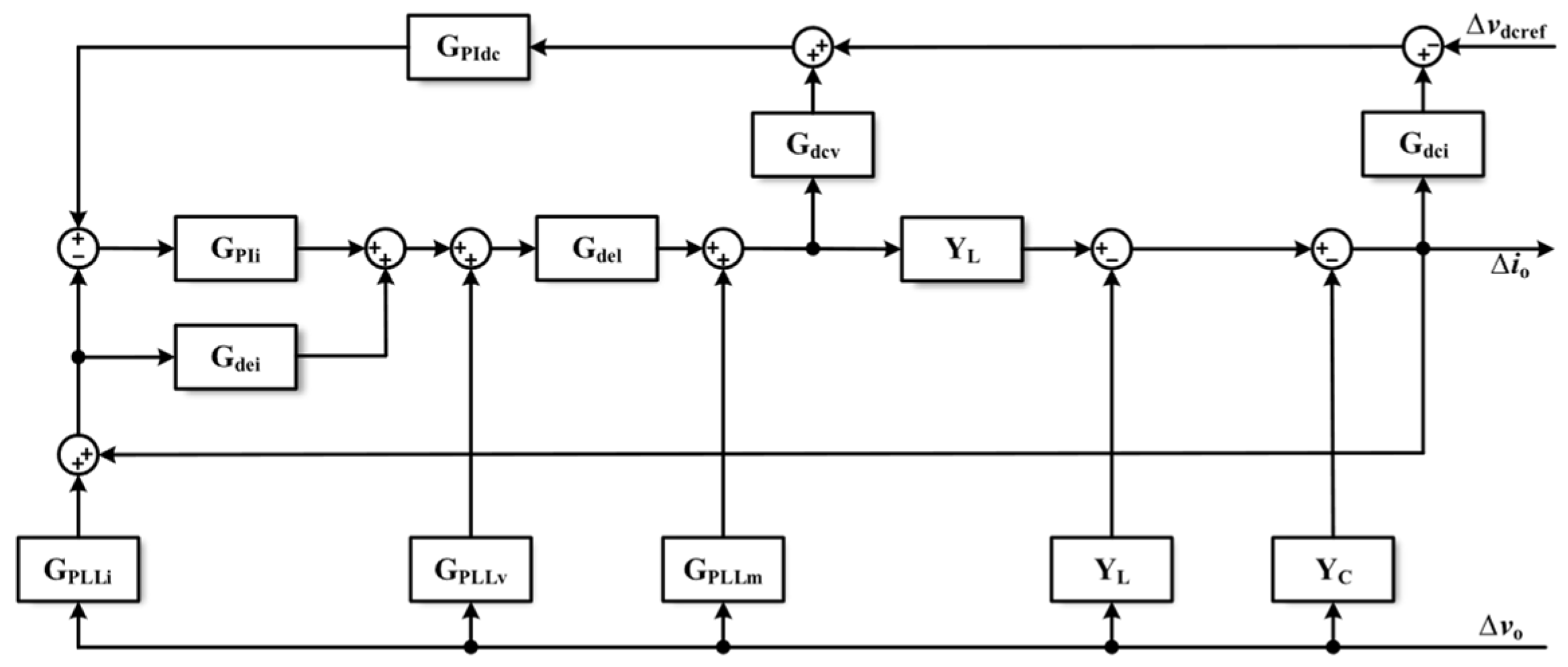
The impedance modeling approach serves as a critical tool for analyzing the small-signal stability of power electronic systems. The dq-frame impedance model of the GFL is depicted in Figure 4, with the detailed derivation process provided in [11,12]. When the active output current of the GFL i_gd is greater than 0, it operates in the inverter mode; when i_gd is less than 0, it operates in the rectifier mode [13].

As illustrated in Figure 4, variables ∆v_o and ∆i_o denote the voltage and current outputs in the dq frame, respectively, and the ratio of A to B yields the output impedance. In the figure, E is the second-order identity matrix. Y_f and Y_c are the admittance matrices of the output LC Filter. G_PIdc and G_PIi are the transfer functions of the voltage and current controllers. G_dei is the current decoupling control matrix, and G_del is the time-delay element matrix. G_dci and G_dcv, respectively, represent the effects of the output current disturbance and the bridge arm voltage disturbance on the DC-side voltage. G_PLLi, G_PLLv, and G_PLLm, respectively, represent the effects of the PLL on the grid-connected current, the PCC voltage, and the bridge arm voltage.

The impedance matrix expression of the GFL is given as follows:

$$\begin{array}{cc}\hfill Z_{\mathrm{GFL}}& ={\left[\begin{array}{c}{Y}_{\mathrm{c}}-Y_{\mathrm{f}}{G}_{\mathrm{del}}{G}_{\mathrm{PIi}}{G}_{\mathrm{PIdc}}{Y}_{\mathrm{c}}-Y_{\mathrm{f}}{G}_{\mathrm{del}}{G}_{\mathrm{pi}}{G}_{\mathrm{pidc}}{G}_{\mathrm{dcv}}{Z}_{\mathrm{f}}{Y}_{\mathrm{c}}+Y_{\mathrm{f}}\\ -Y_{\mathrm{f}}{G}_{\mathrm{del}}{G}_{\mathrm{PIi}}{G}_{\mathrm{PIdc}}{G}_{\mathrm{dcv}}+Y_{\mathrm{f}}{G}_{\mathrm{PLLd}}+Y_{\mathrm{f}}{G}_{\mathrm{del}}\left(G_{\mathrm{PIi}}-G_{\mathrm{dei}}\right)G_{\mathrm{PLLi}}\end{array}\right]}^{-1}\hfill \\ \hfill & \cdot \left[\begin{array}{c}E+Y_{\mathrm{f}}{G}_{\mathrm{del}}\left(G_{\mathrm{PIi}}-G_{\mathrm{dei}}\right)-Y_{\mathrm{f}}{G}_{\mathrm{del}}{G}_{\mathrm{PIi}}{G}_{\mathrm{PIi}}{G}_{\mathrm{PIdc}}{G}_{\mathrm{dci}}\\ -Y_{\mathrm{f}}{G}_{\mathrm{del}}{G}_{\mathrm{PIi}}{G}_{\mathrm{PIdc}}{G}_{\mathrm{dcv}}{Z}_{\mathrm{f}}\end{array}\right]\hfill \end{array}$$

(4)

2.3. Problem Formulation

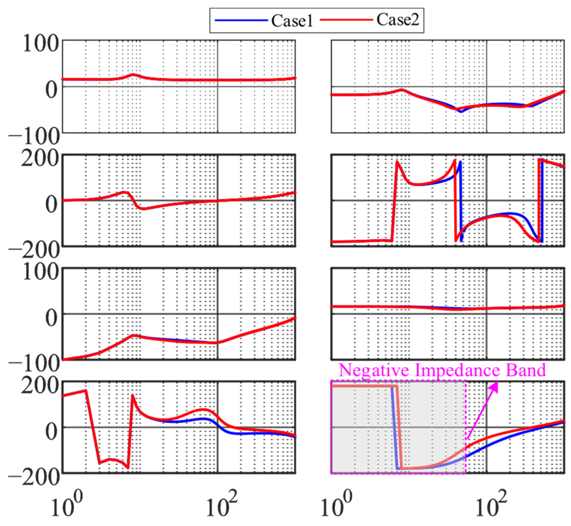
GFL typically behaves as a controlled current source during normal operation and plays a core supporting role in impedance sweep frequency measurement. The GFL realizes high-precision phase synchronization with the power grid via real-time detection of the PCC voltage and PLL operation, providing a stable synchronization reference for impedance–frequency sweeping. Among them, the PI parameters design of the PLL is crucial to synchronization performance and system stability. Figure 5 shows the impedance characteristics of the GFL under inverter mode. Herein, Case 1 (k_ppll = 2, k_ipll = 400) and Case 2 (k_ppll = 1, k_ipll = 200) represent the impedance characteristics corresponding to different control parameters under the system parameters given in Table 1. As can be seen from the figure, improper PLL parameter design will expand the negative impedance region of the qq-axis in inverter mode [14]. The wider the negative impedance frequency band, the more severe the damage to system stability, thereby leading to a decrease in the system’s anti-disturbance capability.

During the impedance measurement phase, the converter injects a set of non-fundamental sinusoidal probing signals covering a wide frequency band into the PCC. This causes the dq impedance of the converter to oscillate near the basic operating condition, which may expand the negative-impedance frequency band at certain moments, reduce the stability of the GFL, and even lead to instability in severe cases. This not only directly threatens the operational stability of the grid-connected system but also causes deviations in oscillation frequency identification, misjudgment in islanding detection, and omission of weak fault characteristics, thereby undermining the reliability of power-grid state assessment and safety protection functions.

Therefore, there is an urgent need to design a PLL method that can maintain stable operation under conditions such as multi-scenario frequency band switching, disturbance enhancement, and harmonic amplification risks. System stability under different frequency sweep scenarios is improved by reshaping the GFL impedance. To address this challenge, this paper proposes an adaptive PLL scheme based on the BP neural network: preset scenario recognition logic for different impedance frequency sweep application scenarios and dynamically adjust PI parameters by combining real-time PCC voltage distortion characteristics and harmonic component monitoring results. This scheme can not only avoid full-frequency-band harmonic amplification caused by improper parameter design but also synchronously improve phase detection accuracy and overall system stability in multi-scenario wide-band frequency sweep measurements, such as oscillation prediction, islanding detection, and weak-characteristic fault diagnosis.

3. Proposed PLL Algorithm for Wide-Frequency Sweep Adaptability

To enhance the operational stability of grid-connected inverters under varying grid conditions, it is necessary to account for the influence of grid impedance on the PCC voltage. Motivated by this requirement, this section focuses on the q-axis component of the PCC voltage and introduces an adaptive PLL enabled by a BP neural network, aiming to strengthen the robustness of synchronization during broadband impedance-sweep operations.

3.1. Control Optimization Architecture

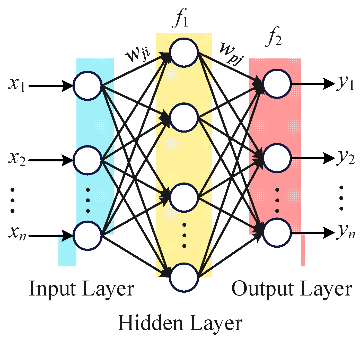
The architecture of the BP neural network is shown in Figure 6. As an artificial intelligence model inspired by biological neural systems, the network is composed of an input layer, a hidden layer, and an output layer. Neurons in each layer are fully interconnected with neurons in adjacent layers, and every connection is assigned a trainable weight. The hidden layer plays a key role in nonlinear feature extraction and functional mapping. By emulating neural information transmission, the BP network updates its weights through the backward propagation of the error between the network output and the target response. This iterative learning mechanism enables the network to achieve accurate nonlinear approximation and ensures convergence of the output toward the desired value [15].

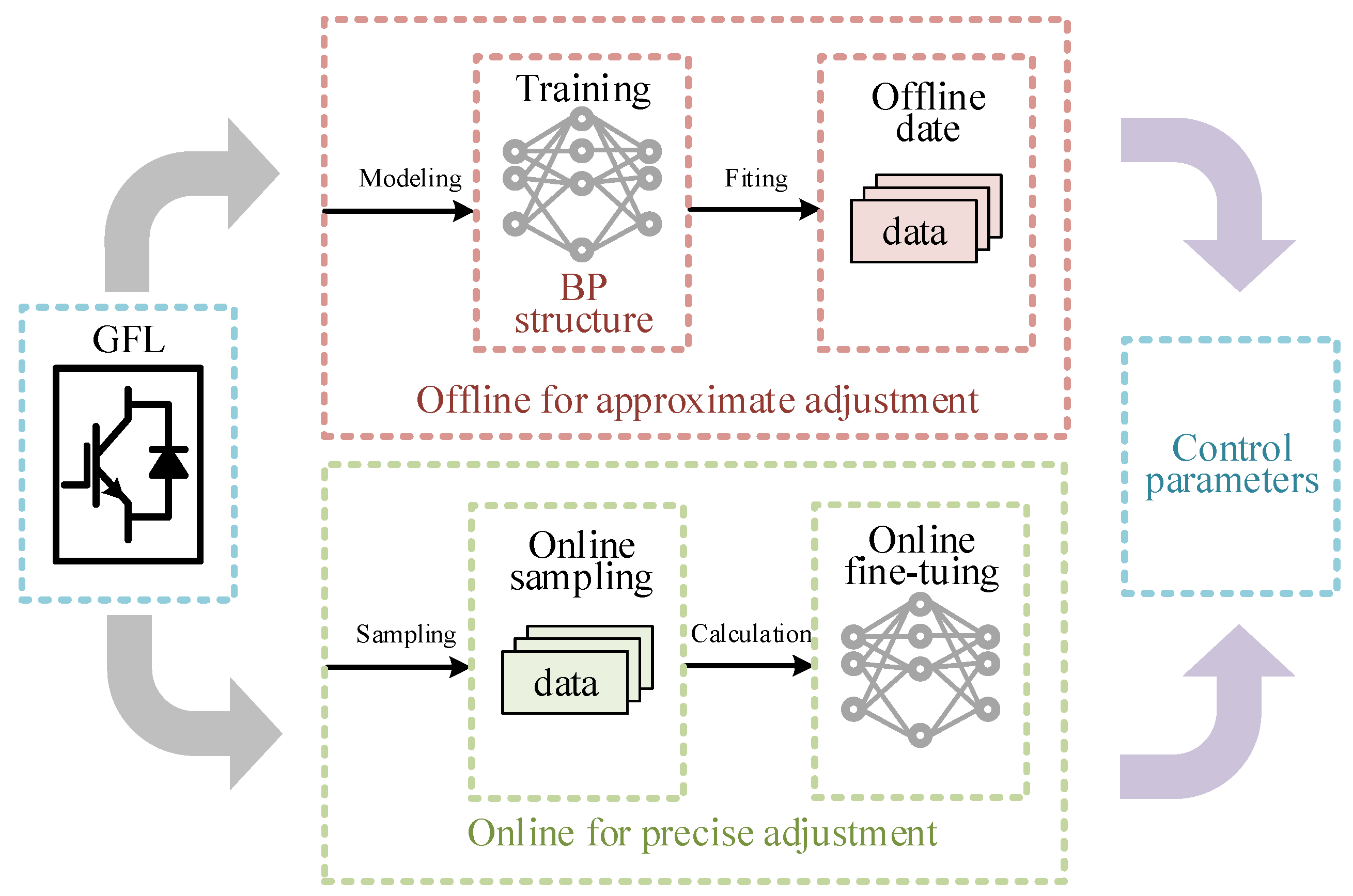
The overall architecture of the control optimization based on the BP neural network proposed in this paper is shown in Figure 7, which is divided into two control layers: an offline layer and an online layer. The offline layer obtains a data mapping set through extensive case training in the early stage and stores it in the processor. It searches for optimal control parameters under different system parameters, providing a fundamental guarantee for system stability. The online layer monitors the changes in system operating conditions in real time and achieves rapid adaptive compensation for dynamic operating conditions with the support of the offline layer.

The offline layer mainly fits the optimal PLL parameters corresponding to different output powers and different SCRs. Since the SCR is difficult to obtain directly, the steady-state voltage deviation at the PCC is adopted to characterize the SCR. The required dataset is acquired from preliminary simulation data and HIL experiments. On this basis, the samples can be further expanded by data transfer, which enables better training of the offline network while ensuring the efficiency of data collection. Through multiple forward and backward propagations of the BP neural network, the mapping relationship between the system parameters and the corresponding control parameters is output. The online layer collects the information of the GFL, calculates the error term by comparing the collected information with the expected value, and computes the parameter variation that minimizes the error based on the gradient descent principle of the BP neural network. Therefore, in contrast to the offline layer, online layer control does not require the support of a dataset.

3.2. Adaptive PLL Based on the BP Neural Network

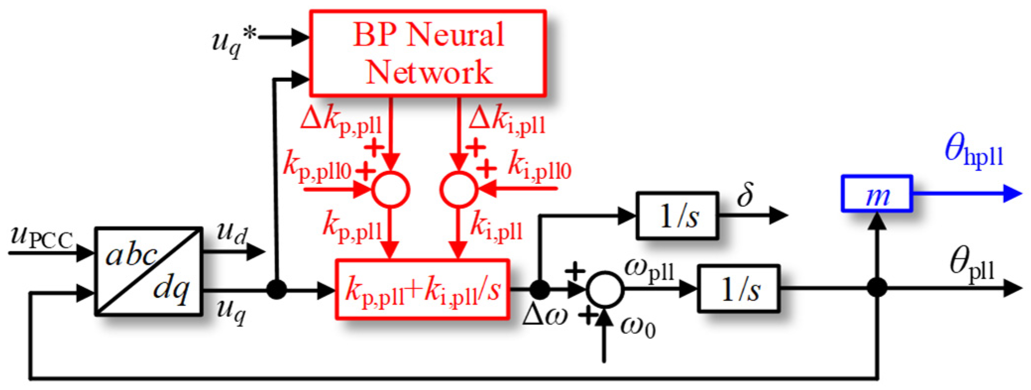
In a conventional SRF-PLL, variations in operating conditions necessitate retuning the proportional and integral gains, k_p,pll and k_i,pll, of the PI regulator—a process that is inherently nonlinear and sensitive to system dynamics. To address this limitation, the proposed method embeds a BP neural network within the PI control structure. Leveraging its nonlinear approximation and adaptive learning capabilities, the neural network provides online gain adjustment for the PLL. The overall framework of the proposed adaptive PLL is depicted in Figure 8. Especially, multiply the power frequency phase angle reference by a factor m to serve as the phase angle reference for non-power frequency signals.

During the online tuning process, a three-layer BP neural network is constructed, where the input layer contains three elements, the hidden layer consists of n neurons, and the output layer contains two elements. The input vector X includes the measured value, the reference value, and the tracking error of the system, whereas the output vector Y represents the parameter increments, ∆k_p,pll and ∆k_i,pll, for the PI controller. The weight matrices between the input and hidden layers and between the hidden and output layers are denoted as W_i and W_o, respectively. Activation functions f₁ and f₂ are employed for hidden and output layers to achieve nonlinear mapping and enable adaptive online adjustment of the PI gains.

The input variables of the system are:

$$\left\{\begin{array}{l}{x}_1=u_q\left(k\right)\hfill \\ x_2=u_q^{*}=0\hfill \\ x_3=e=u_q\left(k\right)-u_q^{*}\hfill \end{array}\right.$$

(5)

Wherein, k denotes the sampling instant, u_q(k) is the actual value, and u_q^∗ is the expected value. The output of the input layer is:

$$x_{\mathrm{out},i}^{\left(1\right)}\left(k\right)=x_i$$

(6)

Wherein, i denotes the i-th element of the input layer vector. The input of the hidden layer activation function is:

$$h_j^{\left(2\right)}\left(k\right)={\displaystyle \sum _{i=1}^3{w}_{ji}^{\left(1\right)}{x}_{\mathrm{out},i}^{\left(1\right)},j=1,2,\dots ,n}$$

(7)

Wherein, h_j⁽²⁾(k) denotes the input signal received by the j-th neuron in the hidden layer, and w_ji⁽¹⁾ is the weight value from the i-th neuron in the input layer to the j-th neuron in the hidden layer. The output of the hidden layer is:

$$x_{\mathrm{out},j}^{\left(2\right)}\left(k\right)={\mathit{f}}_1\left(h_j^{\left(2\right)}\left(k\right)\right)$$

(8)

The input of the output layer activation function is:

$$h_p^{\left(3\right)}\left(k\right)={\displaystyle \sum _{j=1}^n{w}_{pj}^{\left(2\right)}{x}_{\mathrm{out},j}^{\left(2\right)},p=1,2}$$

(9)

In the above equation, h_p⁽³⁾(k) represents the input signal received by the p-th neuron in the output layer, and w_pj⁽²⁾ denotes the weight value from the j-th neuron in the input layer to the p-th neuron in the hidden layer. The output of the output layer is:

$$x_{\mathrm{out},h}^{\left(3\right)}\left(k\right)={\mathit{f}}_2\left(h_p^{\left(3\right)}\left(k\right)\right)$$

(10)

The tuning value output by the BP neural network is:

$$\left\{\begin{array}{c}\Delta k_{\mathrm{p},\mathrm{pll}}=x_{\mathrm{out},1}^{\left(3\right)}\left(k\right)\\ \Delta k_{\mathrm{i},\mathrm{pll}}=x_{\mathrm{out},2}^{\left(3\right)}\left(k\right)\end{array}\right.$$

(11)

To achieve a closed loop within the neural network and enable the network outputs, ∆k_p,pll and ∆k_i,pll, to meet the system requirements through autonomous feedback and weight matrix updates, the mean squared error function is defined as the performance index function:

$$E\left(k\right)={\displaystyle \frac{1}{2}}{e}^2\left(k\right)$$

(12)

Using the gradient descent principle, the weight matrix that minimizes E(k) is sought, with the expectation that the minimum value is found when the gradient is zero. The gradient of E(k) can be expressed as follows:

$${\displaystyle \frac{\partial E\left(k\right)}{\partial {\omega }_{pj}^{\left(2\right)}}}={\displaystyle \frac{\partial E\left(k\right)}{\partial y\left(k\right)}}\cdot {\displaystyle \frac{\partial y\left(k\right)}{\partial u\left(k\right)}}\cdot {\displaystyle \frac{\partial u\left(k\right)}{\partial x_{out,p}^{\left(3\right)}\left(k\right)}}\cdot {\displaystyle \frac{\partial x_{out,p}^{\left(3\right)}\left(k\right)}{\partial h_p^{\left(3\right)}\left(k\right)}}\cdot {\displaystyle \frac{\partial h_p^{\left(3\right)}\left(k\right)}{\partial {\omega }_{pj}^{\left(2\right)}}}$$

(13)

Since ∂y(k)/∂u(k) is difficult to compute directly, the sign function can be adopted as a substitute for ∂y(k)/∂u(k) to simplify the computation:

$${\displaystyle \frac{\partial y\left(k\right)}{\partial u\left(k\right)}}=\mathrm{sgn}\left({\displaystyle \frac{\partial y\left(k\right)}{\partial u\left(k\right)}}\right)=\mathrm{sgn}\left({\displaystyle \frac{y\left(k\right)-y\left(k-1\right)}{u\left(k\right)-u\left(k-1\right)}}\right)$$

(14)

For each expression, through mathematical derivation, the gradient of the mean squared error function can be obtained as follows:

$$\left\{\begin{array}{c}{\displaystyle \frac{\partial E\left(k\right)}{\partial {\omega }_{pj}^{\left(2\right)}}}=-{\delta }_p^{\left(2\right)}\cdot x_{out,j}^{\left(2\right)}(k)\\ {\delta }_p^{\left(2\right)}=e(k)\cdot \mathrm{sgn}\left({\displaystyle \frac{y\left(k\right)-y(k-1)}{u\left(k\right)-u(k-1)}}\right)\cdot {\displaystyle \frac{\partial u\left(k\right)}{\partial x_{out,p}^{\left(3\right)}\left(k\right)}}\cdot f_2^{\prime }(h_p^{\left(3\right)}(k))\end{array}\right.$$

(15)

Let the learning rate be denoted as η and the inertia coefficient as α. The iterative weight values are given as follows:

$$\Delta {\omega }_{pj}^{\left(2\right)}\left(k+1\right)=-\eta {\displaystyle \frac{\partial E\left(k\right)}{\partial {\omega }_{pj}^{\left(2\right)}}}+\alpha \Delta {\omega }_{pj}^{\left(2\right)}\left(k\right)=\eta {\delta }_p^{\left(2\right)}\cdot x_{out,j}^{\left(2\right)}\left(k\right)+\alpha \Delta {\omega }_{pj}^{\left(2\right)}\left(k\right)$$

(16)

Similarly, the update of the weight matrix from the input layer to the hidden layer follows the same logic.

Therefore, the output quantities of the BP neural network controller are ∆k_p,pll and ∆k_i,pll, which are superimposed with the offline tuned, k_p,pll0 and k_i,pll0 to obtain the final control parameters. The current inner loop remains unchanged, and the traditional PI controller in the PLL is replaced with a BP neural network adaptive controller.

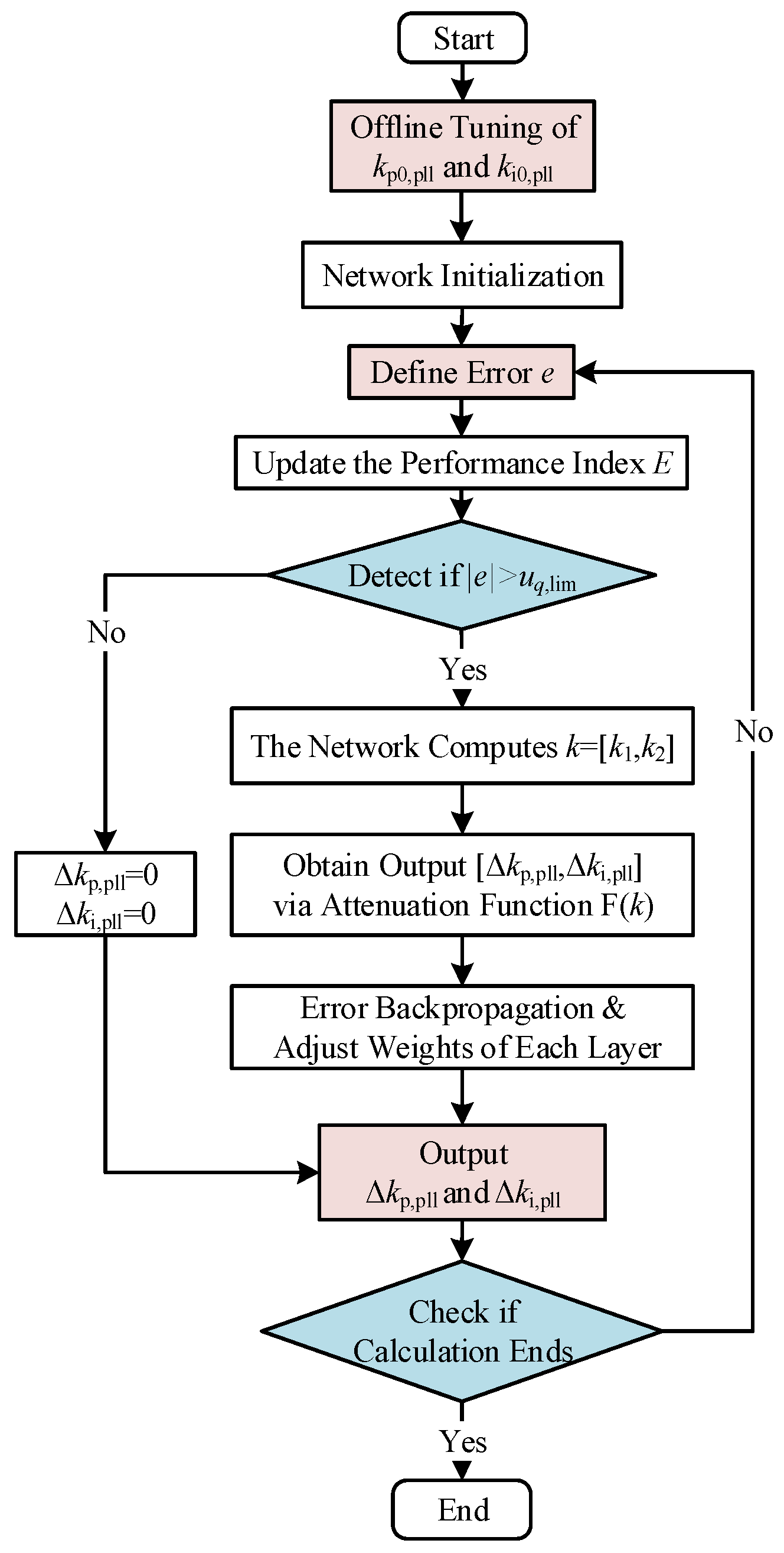
Considering the potential high computational complexity of the BP neural network and the actual power grid conditions, a threshold value u_q,lim is set for u_q. When 0 < |u_q| < u_q,lim, the BP neural network module ceases operation and maintains the adjusted outputs of ∆k_p,pll and ∆k_i,pll. Considering that a larger u_q requires larger ∆k_p,pll, and ∆k_i,pll to facilitate system stability, a positively correlated function F(u_q) with respect to |u_q| can be finally introduced as the coefficient for the outputs ∆k_p,pll and ∆k_i,pll to further improve the computational speed. The system flow chart is shown in Figure 9.

Since the commonly used activation functions in the BP neural network are in the form involving natural exponents, the third-order saturated polynomial can be adopted to approximate the ideal activation function and its derivative for the sake of reducing the computational load. Assuming the number of neurons in the input, hidden, and output layers of the online BP neural network is a, b, and c, respectively, the computational complexity of online computation becomes O(a × b + b × c) after all complex operations are approximately converted into the corresponding addition, subtraction, multiplication, and division operations. The operation speed in controllers such as DSP can be greatly improved by appropriately designing the number of neurons in the hidden layer. In addition, the PI control inherently has a certain dynamic response time, so the update of the online layer does not need to be too frequent and can be set to one-tenth of the switching frequency.

4. Performance Evaluation

4.1. Small-Signal Stability Analysis

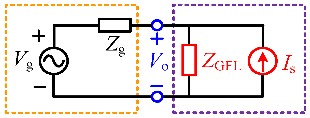
The impedance-modeling-based stability analysis method was first proposed by Middlebrook. According to Thevenin’s theorem, the source subsystem can be equivalent to an ideal voltage source in series with its output impedance. By virtue of Norton’s theorem, the load subsystem can be represented as an ideal current source in parallel with its input impedance, where the system stability is determined by the impedance ratio of the subsystems. Currently, this method has been extended to evaluate the stability of grid-connected converters. Specifically, the GFL is equivalent to an ideal current source I_s in parallel with its output impedance Z_GFL, while the grid side is modeled as an ideal voltage source V_g in series with the grid impedance Z_g, as shown in Figure 10 [16].

$$Z_{\mathrm{g}}=\left[\begin{array}{cc}{R}_{\mathrm{g}}+s{L}_{\mathrm{g}}& -\omega L_{\mathrm{g}}\\ \omega L_{\mathrm{g}}& R_g+s{L}_{\mathrm{g}}\end{array}\right]$$

(17)

It can be observed from Figure 10 that the transfer function expression of the GFL grid-connected system is given as follows:

$$V\left(s\right)={\left[E+Z_{\mathrm{g}}\left(s\right)Z_{\mathrm{GFL}}^{-1}\left(s\right)\right]}^{-1}\left[I_{\mathrm{s}}\left(s\right)Z_{\mathrm{g}}\left(s\right)+V_{\mathrm{g}}\left(s\right)\right]$$

(18)

Assuming that both the output current of the GFL and the grid voltage maintain stability, and the grid impedance has no right-half-plane poles, variables I_s, V_g, and Z_g are thus guaranteed to be stable under such circumstances, with the overall system stability dominated by H(s).

$$H\left(s\right)={\left[E+Z_{\mathrm{g}}\left(s\right)Y_{\mathrm{GFL}}\left(s\right)\right]}^{-1}$$

(19)

H(s) represents the transfer function of a negative feedback closed-loop system where the feedforward gain is an identity matrix, and the feedback gain is Z_gY_GFL. The system remains stable when the negative feedback gain satisfies the Generalized Nyquist Criterion (GNC). The eigenvalue expression of the feedback gain is given as follows:

$$\left\{\begin{array}{c}{Z}_{\mathrm{g}}\left(s\right)Y_{\mathrm{GFL}}\left(s\right)=\left[\begin{array}{cc}{G}_{\mathrm{kdd}}& G_{\mathrm{kdq}}\\ G_{\mathrm{kqd}}& G_{\mathrm{kqq}}\end{array}\right]\\ {\lambda }_{1,2}={\displaystyle \frac{G_{\mathrm{kdd}}+G_{\mathrm{kdq}}}{2}}\pm \sqrt{{\left({\displaystyle \frac{G_{\mathrm{kdd}}-G_{\mathrm{kdq}}}{2}}\right)}^2+G_{\mathrm{kdq}}{G}_{\mathrm{kqd}}}\end{array}\right.$$

(20)

When the Bode plot is adopted to analyze the stability of the GFL grid-connected system, it is necessary to investigate the phase margin and gain margin of eigenvalue λ_1,2. The larger the phase margin and gain margin, the higher the stability of the system.

In addition, the system stability can also be analyzed by investigating the pole distribution of the closed-loop transfer function H(s). The calculation formula is given as follows:

$$\det \left(E+Z_{\mathrm{g}}\left(s\right)Y_{\mathrm{GFL}}\left(s\right)\right)=0$$

(21)

If the eigenvalue H(s) has poles located in the right-half plane, the system becomes unstable. If all poles of the eigenvalue H(s) lie in the left-half plane, the system remains stable.

4.2. Stability Analysis

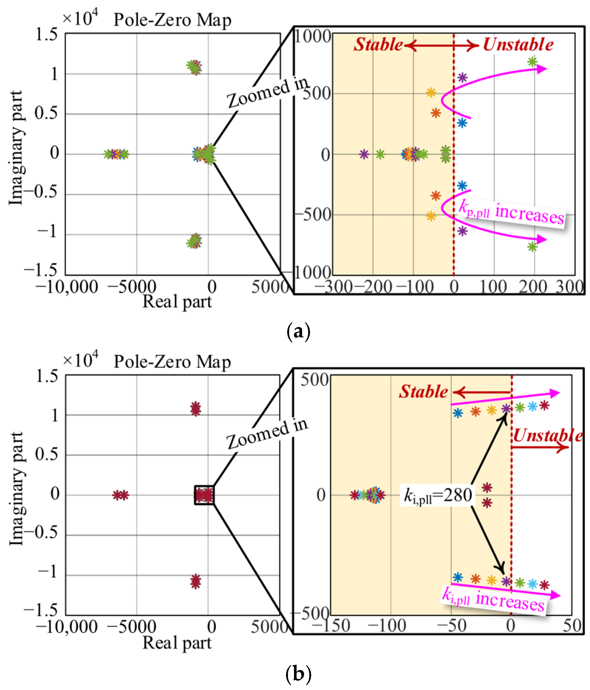
Figure 11 depicts the root loci of the model under different PLL parameters. As shown in Figure 11a, when k_p,pll = 0.5, the real part of the dominant poles of the system is positive, which means that the system is unstable. When k_p,pll increases to 1 or 1.5, the system can maintain small-signal stability. However, when k_p,pll increases to 2, the dominant poles cross the imaginary axis from left to right. Therefore, it can be obtained that, too large or too small k_p,pll will deteriorate the system stability. In addition, as depicted in Figure 11b, the dominant poles move towards the imaginary axis with k_i,pll increases, and finally cross the imaginary axis at about k_i,pll = 280, i.e., the system becomes unstable if k_i,pll is larger than 280. Thus, it can be concluded that larger k_i,pll will worsen the small-signal stability.

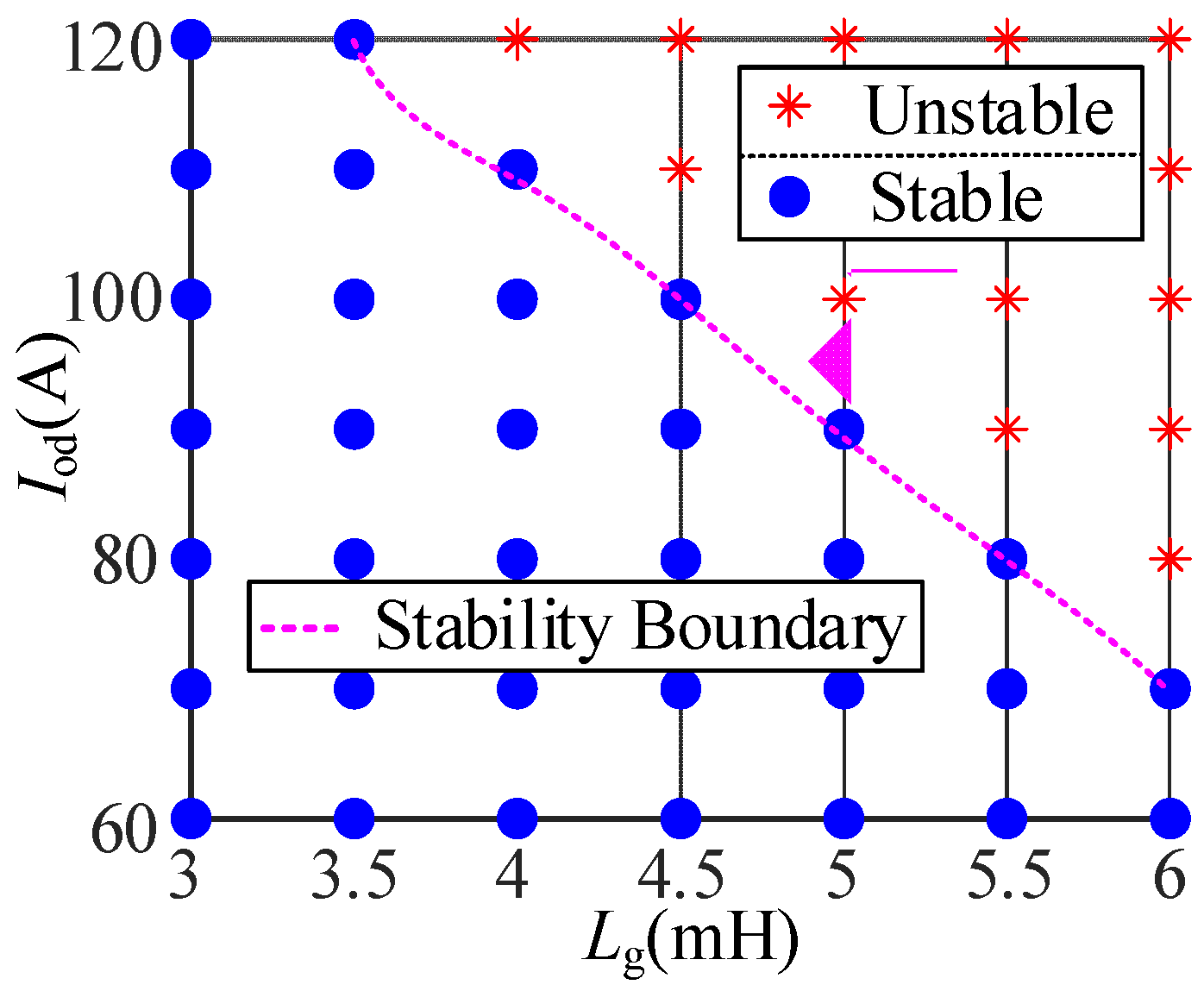
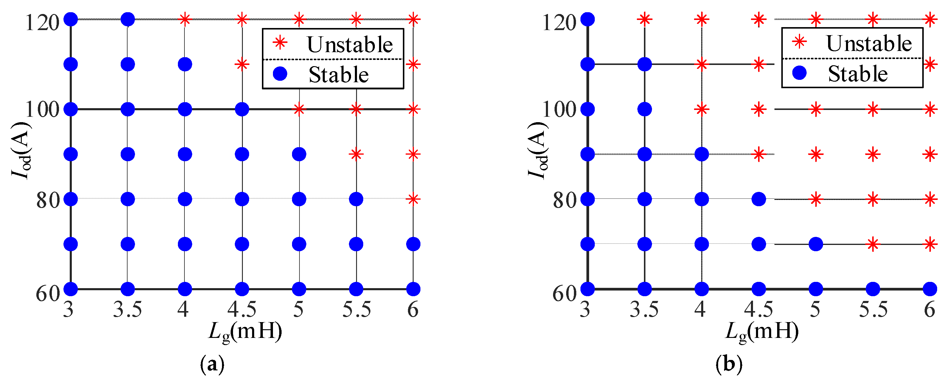
To quantitatively illustrate the inverter parameter influence on the small-signal stability, the stability region can be depicted. Figure 12 shows the small-signal stability regions of the linearized model with different L_g and active current reference I_od, other parameters following Table 1. In Figure 12a with k_i,pll = 2 and k_i,pll = 200, It can be seen that larger L_g and I_od (i.e., smaller SCR values) are not conducive to the small-signal stability in weak grid. Moreover, in Figure 12b with k_i,pll = 2 and k_i,pll = 400 (i.e., k_i,pll increases), the stability region shrinks compared with Figure 12a. Thus, tuning the PLL parameters appropriately is essential to the system stability.

Reducing the PLL integral coefficient k_i,pll can improve system stability, but an excessively large or small proportional coefficient k_p,pll is detrimental to stability. Therefore, it is urgent to adopt the proposed PLL scheme to dynamically and adaptively adjust the PI parameters. Based on the above analysis, it can be concluded that when the adaptive PLL is adopted to dynamically adjust the control parameters, the proportional gain and integral gain can be reduced, thus enabling the BP neural network to search for the optimal value within the preset range. Although the existing stability analysis is based on the impedance model with fixed parameters, it can be concluded that the system stability boundary shifts upward and the stable domain expands after imposing constraints on the output of the BP neural network with the incorporation of adaptive control. A schematic diagram is presented in Figure 13. As can be seen from the analysis of Figure 11, reducing the proportional gain and integral gain will shift the characteristic roots to the left half-plane, which corresponds to an increase in the damping ratio of the dominant poles. This enhances the system’s disturbance rejection capability and is conducive to improving the small-signal stability margin.

Since the online computation part of the BP neural network is updated in real time, the BP neural network is equivalent to a dynamic element in the model for further analysis. As analyzed in Section 3, the simplified computational complexity of the online BP neural network is O(a × b + b × c). The time required for a single floating-point operation in a DSP chip is approximately 5–10 ns, and the time for a single online update is roughly estimated to be 1 μs. The computation process of the BP neural network is equivalent to a time delay of 1 μs, which is analyzed qualitatively in combination with the parameter optimization idea in this section.

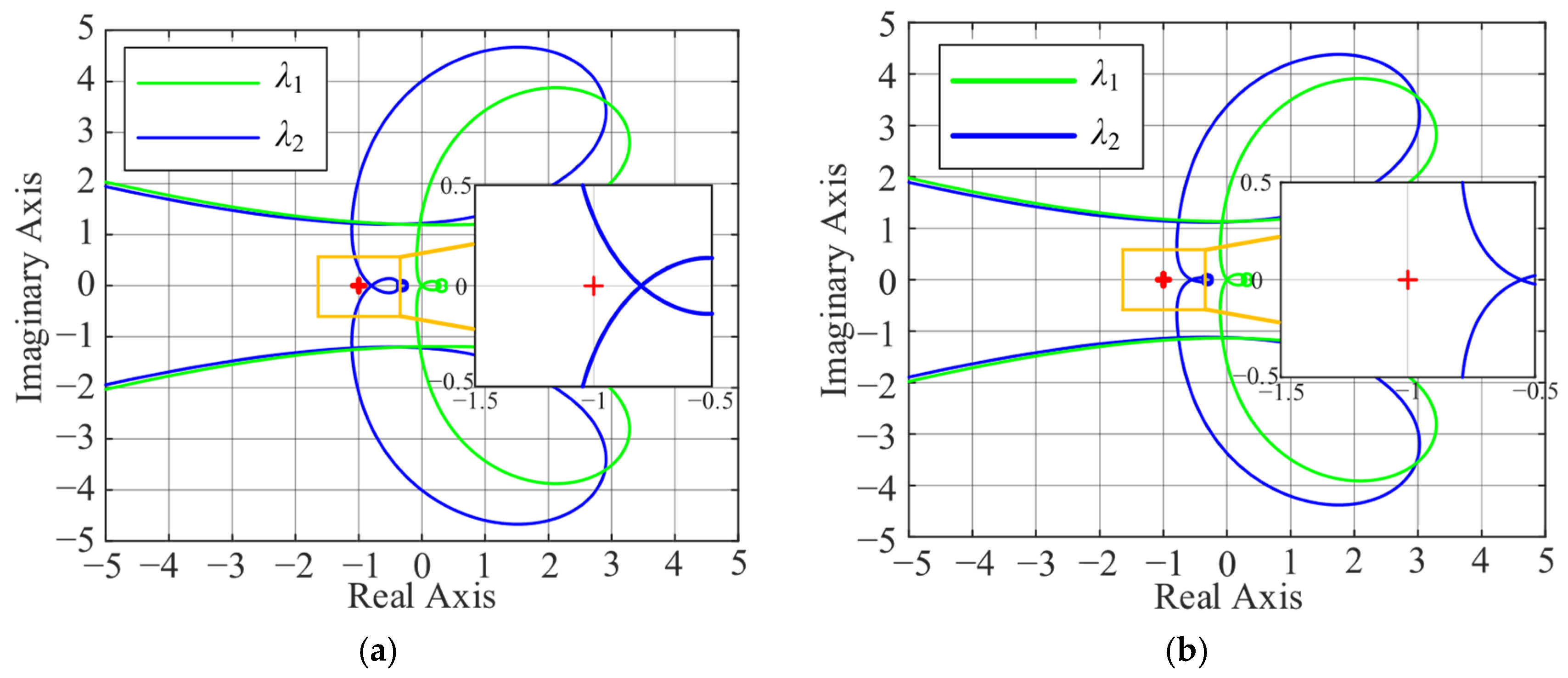
Figure 14 presents a comparison of the system Nyquist diagrams for the conventional PLL and the PLL with BP dynamics considered. The stability margin of the system is enhanced with the incorporation of the BP neural network.

5. Simulation and Experimental Results

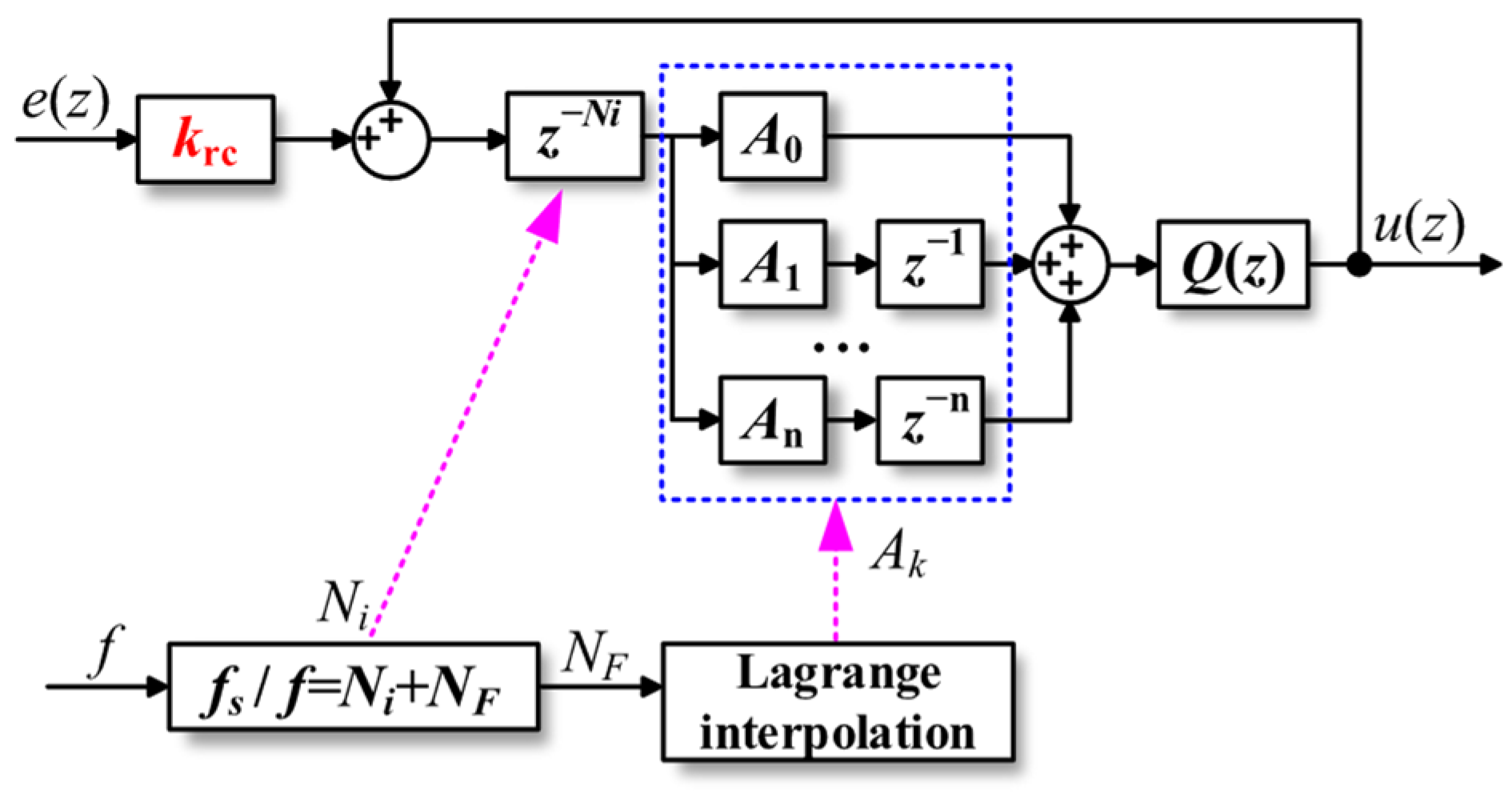
To verify the effectiveness of the proposed adaptive PLL, both simulation and experimental validations are conducted. The system model is shown in Figure 2, and the system parameters are listed in Table 1. Among them, a GFL is used for disturbance signal injections to support the system in completing impedance sweeping. It is worth noting that the phase reference of the disturbance signal is also provided by the improved PLL, as shown in Figure 8. DC voltage tracking is implemented by a PI controller. Fundamental frequency current tracking is achieved in the dq coordinate system using a PI controller. Tracking of non-fundamental frequency current is realized in the dq coordinate system through the parallel connection of a proportional controller and a Fractional-Order Repetitive Control (FORC) [17]. Figure 15 shows the block diagram of the FORC.

The controller parameters are listed in

Table 2. Control parameters.

Symbol	Parameters	Value
kpdc	DC voltage proportional gain	0.5
kidc	DC voltage integral gain	20
kpc	50 Hz current proportional gain	5
kic	50 Hz current integral gain	500
kprc	non-fundamental frequency Current proportional gain	5
krc	Resonant gain	1
kp,pll0	PLL proportional gain	1
ki,pll0	PLL integral gain	200

. Based on the existing stability analysis, it can be considered that excessively large values of both k_p,pll and k_i,pll are detrimental to system stability. When the adaptive PLL is adopted, the PI ranges output by the BP neural network are specified as [0.1–k_p,pll0,0] and [1–k_i,pll0,0], respectively. While considering stability optimization, the problems of excessively slow regulation or negative values caused by excessively small PLL parameters can be avoided. In the simulation verification, the number of neurons in the input layer, hidden layer, and output layer of the backpropagation (BP) neural network is set to 3, 7, and 2, respectively. The update frequency of the BP neural network is one-tenth of the switching frequency.

5.1. Simulation Results

A system simulation model is established in MATLAB/Simulink (R2025a) with the assistance of PLECS, with the basic parameters consistent with those in Table 1. Set the DC-side voltage of the GFL to 1200 V. The equivalent resistance between the DC source and the GFL is 5 Ω.

First, the basic functions of the GFL operating in inverter mode need to be verified. In this test, the DC-side voltage reference (V_dcref) is set to 1060 V, the output reactive current reference to 0. The system output waveforms are given as follows.

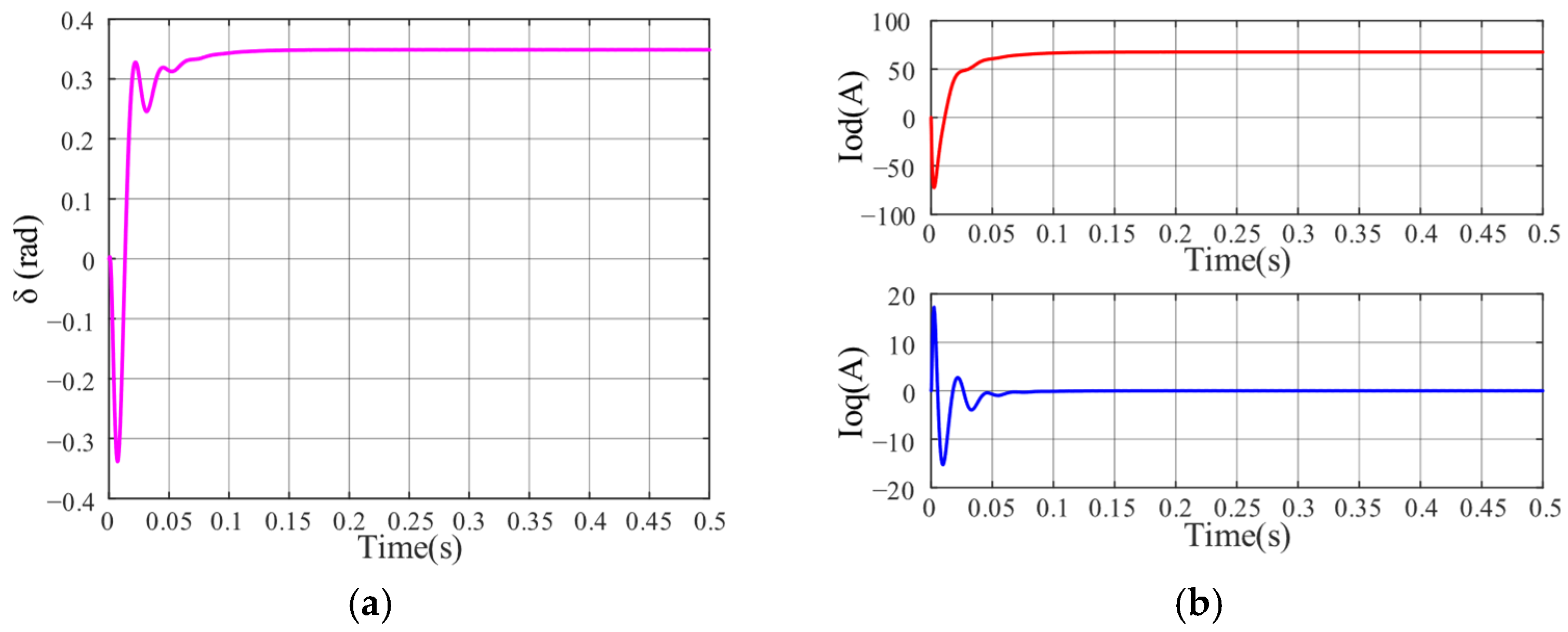
As illustrated in Figure 16, the system operates under basic inverter mode with no harmonic injection. After startup, the system responds rapidly, and both the active and reactive currents reach their theoretical steady-state values. The power angle also stabilizes at a steady value, which verifies the realization of the GFL’s basic functions.

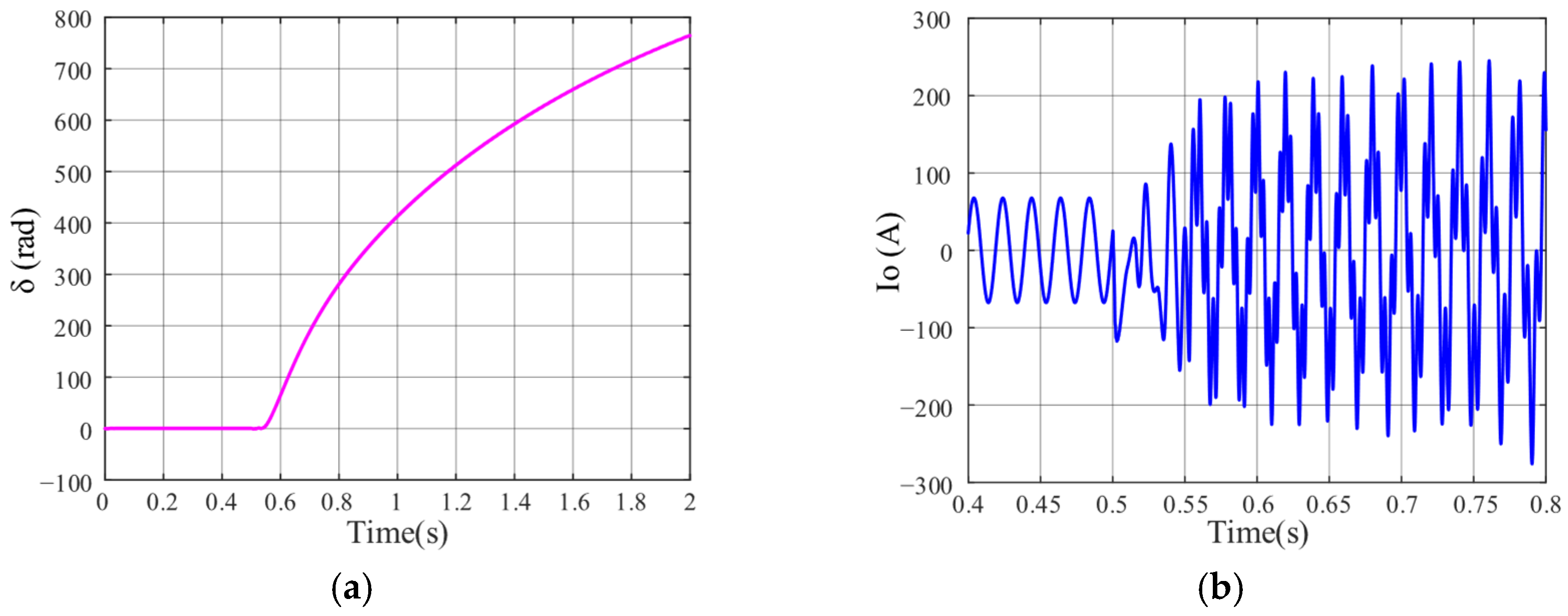
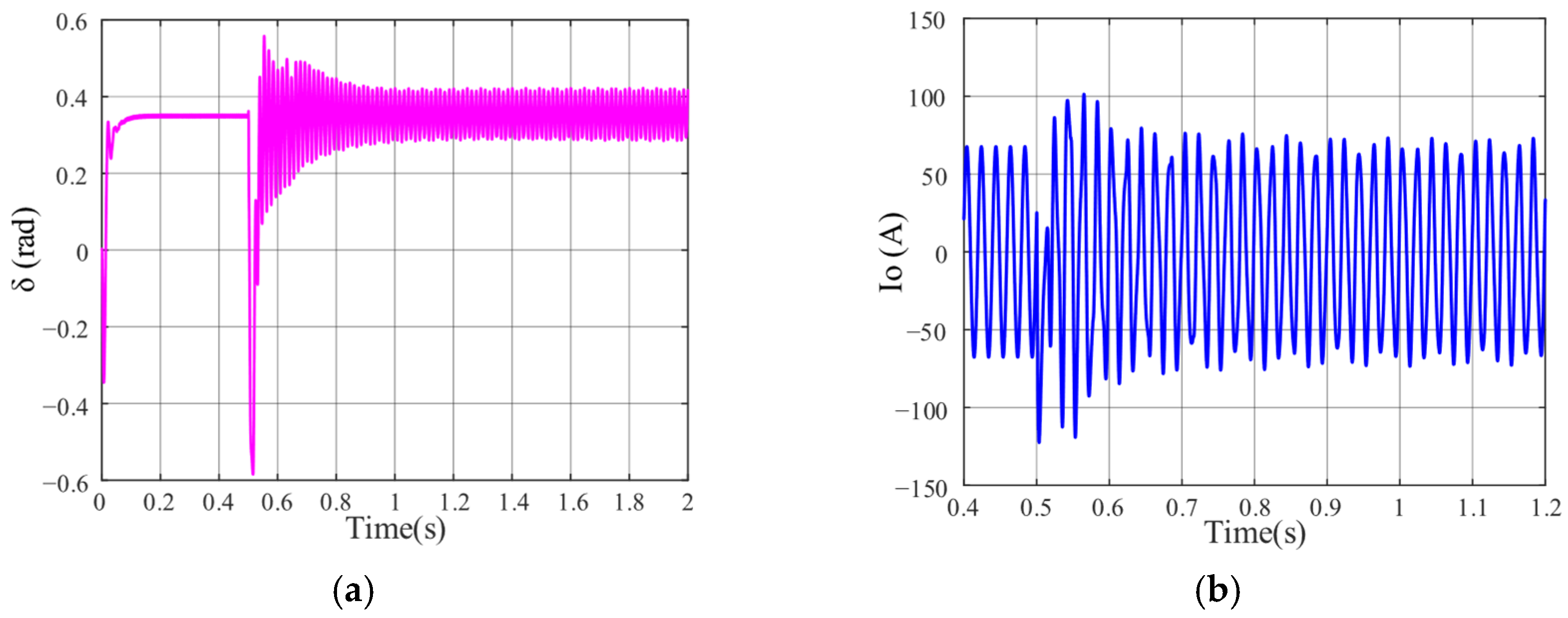
Next, the non-fundamental frequency harmonic injection function under the impedance sweeping scenario is integrated into the GFL control system. It is set that when the system operates for 0.5 s. The GFL injects a non-fundamental frequency harmonic with a frequency of 115 Hz and an amplitude of 5 A. The SRF-PLL and the adaptive PLL proposed in this paper are respectively adopted for phase locking, and the simulation results are presented as follows.

As can be observed from Figure 17, no disturbance signal is injected during the initial operation phase. At 0.5 s, a disturbance is injected into the grid side by the GFL. The system exhibits a divergent tendency after being disturbed. The power angle of the PLL increases continuously, and the system fails to converge to the equilibrium point. At the moment of disturbance, the current has an impulse response with no tendency to stabilize. In conclusion, when the system injects non-fundamental signals, the traditional PLL is affected by disturbances, leading to system instability, and its stability needs to be further improved.

As can be observed from Figure 18, no disturbance signal is injected during the initial operation phase. The adaptive PLL detects the normal PCC voltage and maintains the PI parameters of the PLL unchanged, indicating that the adaptive PLL exerts no impact on the system under steady-state conditions. At 0.5 s, a disturbance is injected into the grid side by the GFL. Compared with the conventional PLL, the adaptive PLL responds promptly upon detecting the abnormal voltage at the PCC. After calculation, k_p,pll and k_i,pll are finally adjusted to 1 and 129, respectively, and the system resumes stable operation. The power angle of the PLL converges again after a short transient process, and the system output current is maintained at a steady-state value.

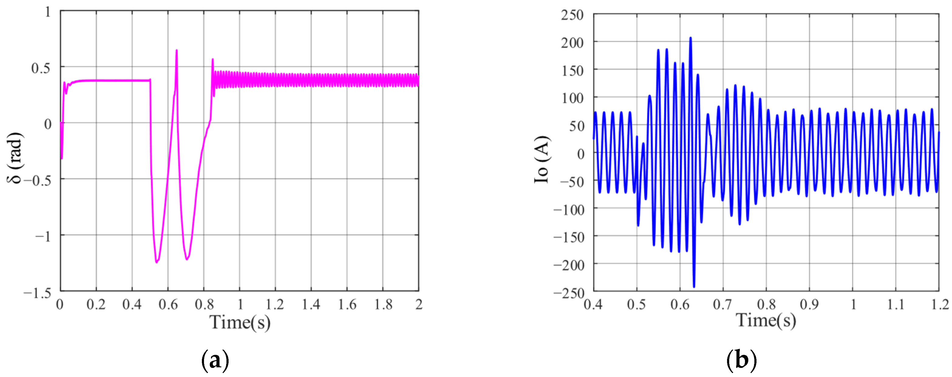
To further verify the effectiveness of the proposed scheme under different operating conditions, the DC-side reference voltage of the system is adjusted to 1050 V. In this case, the theoretical output active current increases, the system moves toward the instability region, and its stability deteriorates further.

As can be observed from Figure 19, the system continues to drift toward the instability region, and non-fundamental frequency harmonic injection is enabled at 0.5 s. The adaptive PLL can still respond rapidly; through calculation, it finally adjusts k_p,pll and k_i,pll to 0.69 and 132, respectively, and the system returns to stable operation. The proposed adaptive PLL can enhance system stability, verifying the effectiveness of the proposed PLL scheme.

5.2. Experimental Results

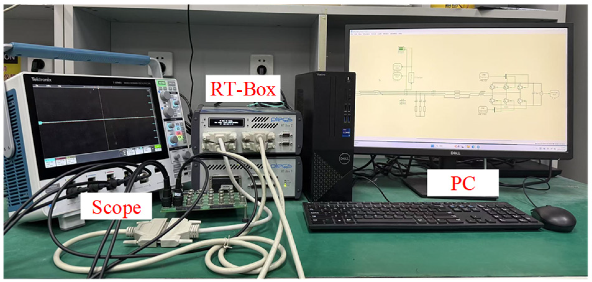
To further verify the effectiveness of the proposed adaptive phase-locking scheme, experimental validation is conducted using the HIL test bench shown in Figure 20. The GFL is implemented in the RT-BOX, with its structure illustrated in Figure 2 and Figure 8. The PWM carrier frequency is set to 10 kHz, and the switching delay is 1 μs.

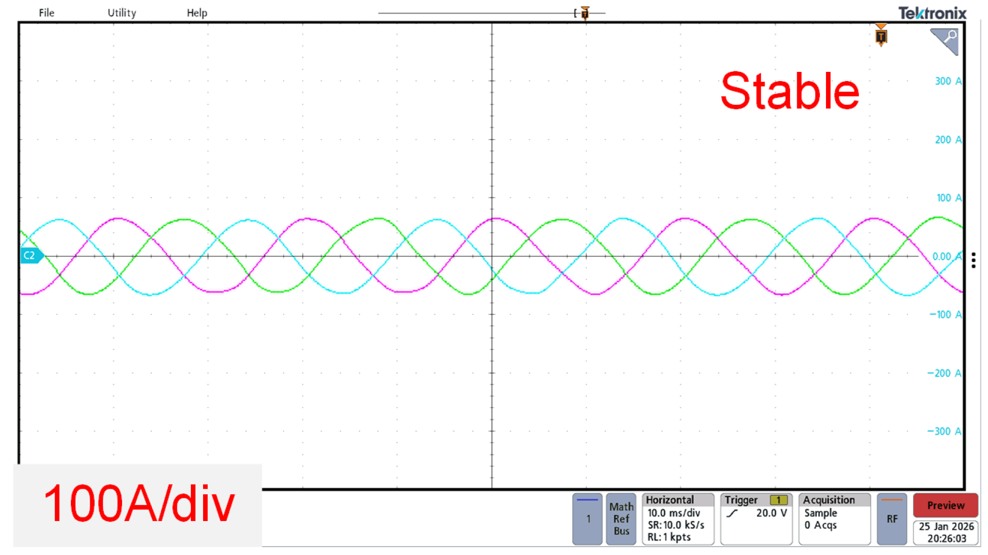
First, set the GFL DC-side reference voltage to 1060 V. The current output waveform under basic inverter mode is shown in Figure 21, with the system operating in a stable state. The blue, purple, and green waveforms represent the three-phase currents output by the converter. The same below Figure 22, Figure 23 and Figure 24.

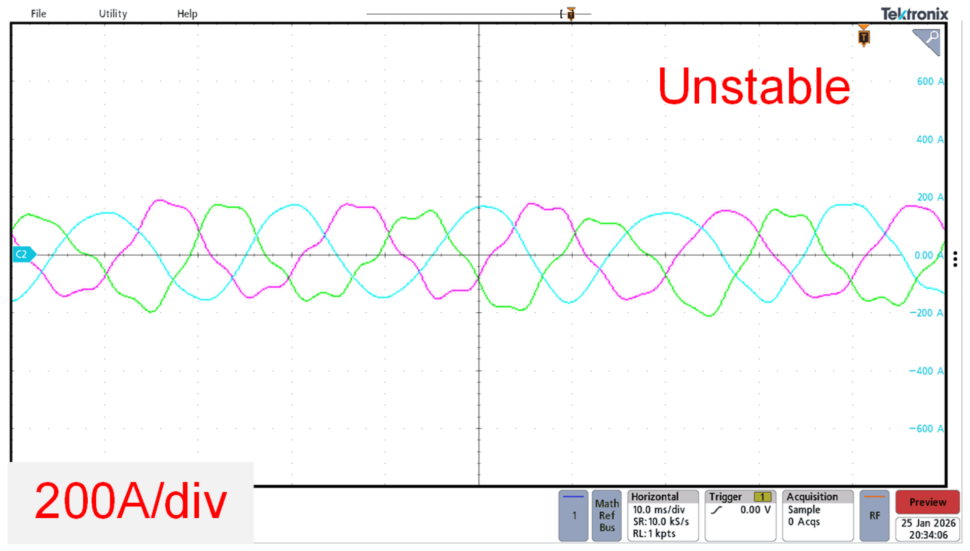
k_p,pll0 and k_i,pll0 are set to 1.2 and 200, respectively. Other initial parameters of the system are listed in Table 1 and Table 2. The injected current is set to a frequency of 115 Hz and an amplitude of 5 A, and the current waveform under the initial PLL parameters is depicted in Figure 22. The GFL becomes unstable rapidly with harmonic injection.

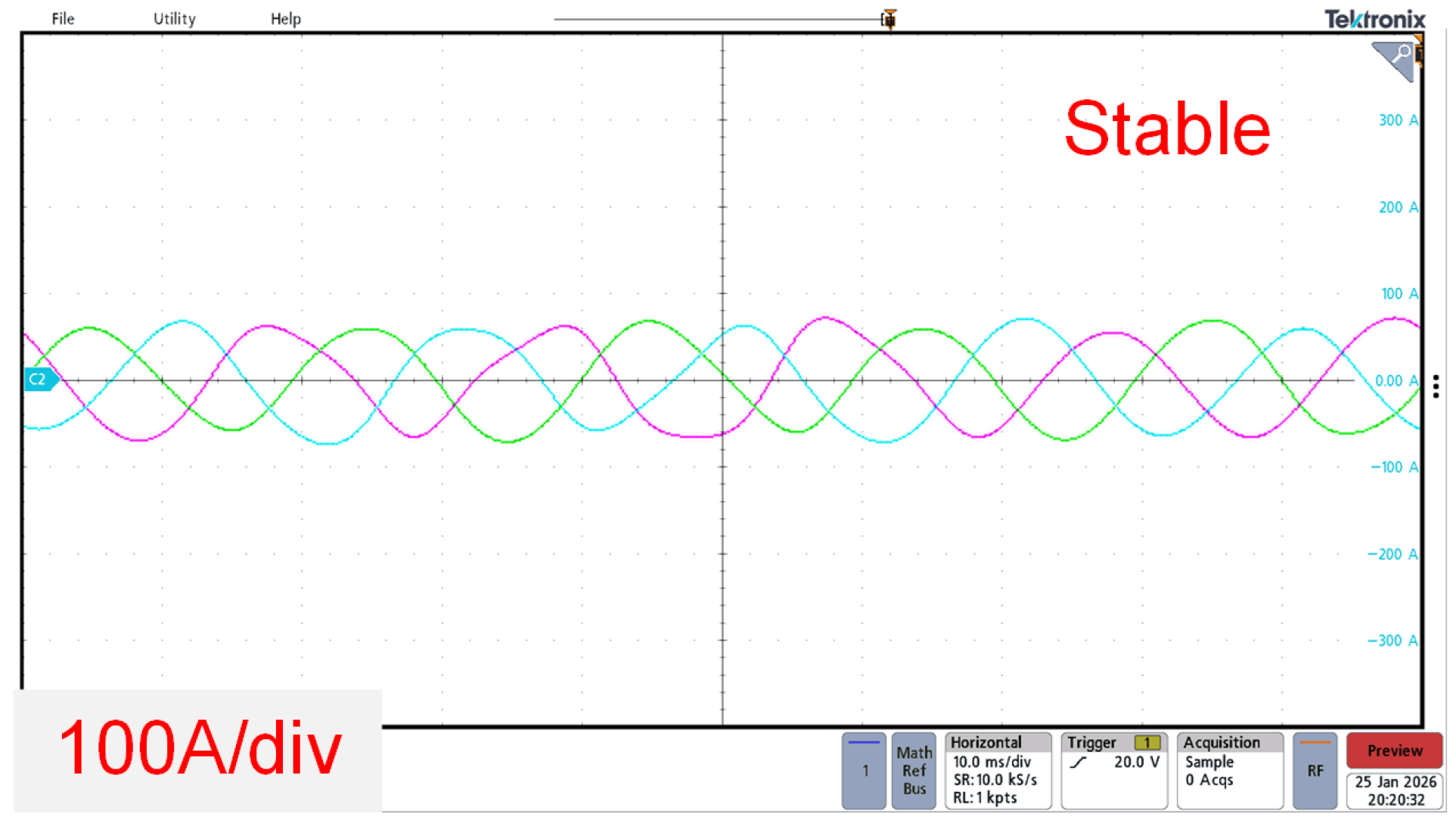
Subsequently, the conventional PLL is replaced with the proposed adaptive PLL, and the online layer of the BP neural network detects and adjusts the control parameters in real time. The GFL output current waveform is shown in Figure 23. Despite harmonic injection, the output current remains in a stable state.

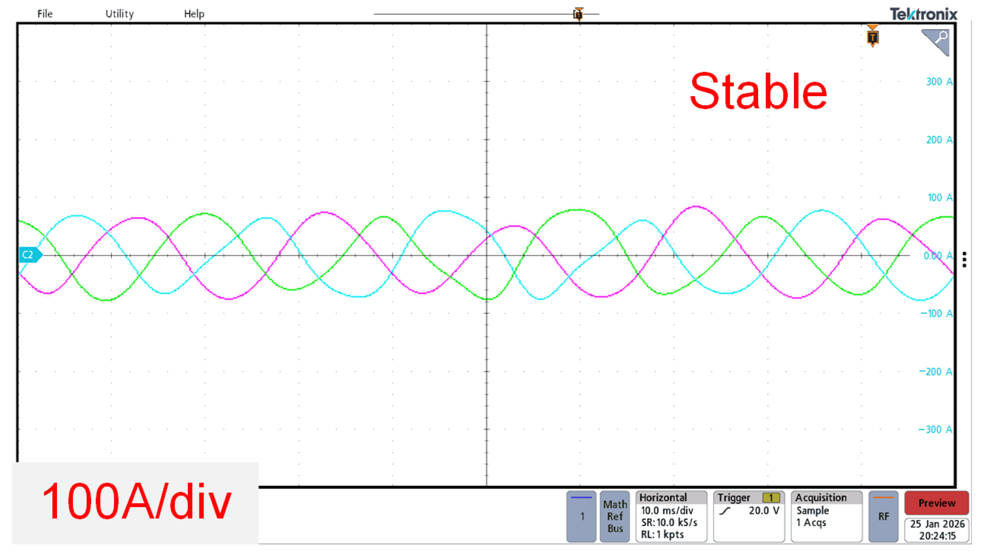
Finally, to further verify the accuracy of the study, the GFL reference voltage is set to 1050 V with other parameters unchanged. This means the output active-current increases, and the GFL will shift toward the instability region. The same 115 Hz, 5 A non-fundamental frequency harmonics are injected. The GFL output-current waveform is shown in Figure 24. The results demonstrate that the GFL converter can maintain a stable operating state even with harmonic injection, which further verifies the effectiveness of the method proposed in this paper.

In Figure 23 and Figure 24, although the total harmonic distortion (THD) of the injected current appears relatively high, this paper focuses on investigating the stability of harmonic injection under frequency-sweep scenarios. For operation in an actual power grid, small-amplitude harmonics should be injected in accordance with grid codes. Since the system can maintain stability with large-amplitude harmonic injection, it will remain stable when the injected harmonics are replaced with small-amplitude ones.

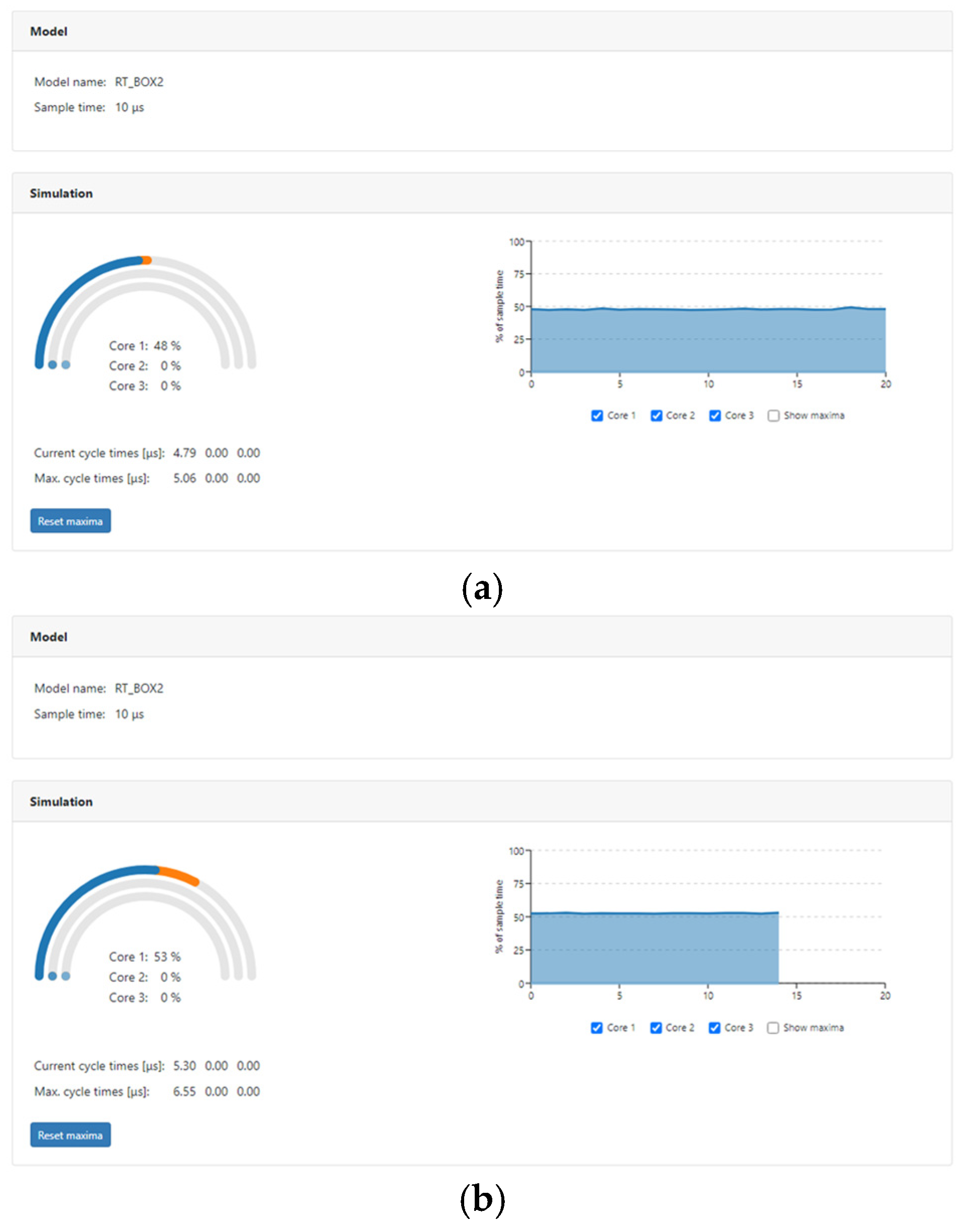
In addition, the execution time of the online computation of the BP neural network is estimated in the HIL experiments. The sampling time is 10 μs. Figure 25a depicts the execution performance with the conventional PLL, with a CPU utilization rate of 48%. Figure 25b depicts the execution performance with the proposed adaptive PLL, with a Core utilization rate of 53%. A comparison indicates that the online computation time of the BP neural network is approximately 0.5 μs, and its impact on the system stability is negligible. The experimental results are basically consistent with the analyses in Section 3 and Section 4.

6. Conclusions

This paper proposes an adaptive phase-locked loop (PLL) scheme based on a BP neural network for grid-following converters operating under frequency-sweep–based impedance measurement. By exploiting the nonlinear mapping and adaptive learning capabilities of the neural network, together with a hybrid strategy combining offline parameter tuning and online adaptive adjustment, the proposed method effectively enhances synchronization robustness and system adaptability under dynamic operating conditions. The proposed PLL satisfies the synchronization requirements of impedance frequency-sweeping scenarios without the need for additional hardware modifications. Both simulation studies and experimental results validate the effectiveness of the proposed scheme.

It should be noted that the proposed method exhibits certain limitations in practical applications. First, the offline tuning process relies on sufficiently comprehensive training data to ensure reliable performance. Second, online adaptive adjustment introduces higher computational complexity compared with conventional PLL schemes, thereby imposing increased requirements on controller hardware. To address these challenges, future work will focus on constructing a more extensive training dataset, optimizing the neural network architecture and computational efficiency, and further enhancing adaptability across a wider range of operating conditions. In addition, the proposed approach can be extended to the investigation of converter transient stability under disturbed grid conditions.

References

1. Wang, X.; Blaabjerg, F. Harmonic stability in power electronic-based power systems: Concept, modeling, and analysis. IEEE Trans. Smart Grid 2019, 10, 2858–2870. [Google Scholar] [CrossRef] [Scilit]
2. Rong, Q.; Hu, P.; Yu, Y.; Wang, D.; Cao, Y.; Xin, H. Virtual External Perturbance-Based Impedance Measurement of Grid-Connected Converter. IEEE Trans. Ind. Electron. 2025, 72, 2644–2654. [Google Scholar] [CrossRef] [Scilit]
3. Guo, Z.; Zhang, X.; Chen, Q.; Wang, M.; Li, M.; Wang, H. An impedance identification-based islanding detection method for droop control inverters based on RDFT and positive–negative notch filters. Energy Rep. 2022, 8, 1060–1070. [Google Scholar] [CrossRef] [Scilit]
4. Zhou, W.; Ravanji, M.H.; Mohammed, N.; Bahrani, B. Rapid Admittance Measurement of Power Converters Using Double-PLL Grid-Following Inverters. IEEE Trans. Power Deliv. 2024, 39, 1407–1419. [Google Scholar] [CrossRef] [Scilit]
5. Yang, D.; Wang, X.; Liu, F.; Xin, K.; Liu, Y.; Blaabjerg, F. Symmetrical PLL for SISO Impedance Modeling and Enhanced Stability in Weak Grids. IEEE Trans. Power Electron. 2020, 35, 1473–1483. [Google Scholar]
6. Eskandari, M.; Savkin, A.V.; Alhelou, H.H.; Blaabjerg, F. Explicit Impedance Modeling and Shaping of Grid-Connected Converters via an Enhanced PLL for Stabilizing the Weak Grid Connection. IEEE Access 2022, 10, 128874–128889. [Google Scholar] [CrossRef] [Scilit]
7. Shang, L.; Hua, Z.; Liu, C.; Dong, X. Amplitude-Phase-Locked-Loop-Based Power Injection Strategy for Wind Power Generation Under Three-Phase Grid Fault. IEEE Trans. Energy Convers. 2022, 374, 2952–2961. [Google Scholar] [CrossRef] [Scilit]
8. Qin, C.; Gao, F.; Wang, G.; Nie, K. Data-driven Multi-parameter Tuning for Stabilizing Grid-following Inverters. IEEE Trans. Power Electron. 2025. [Google Scholar] [CrossRef] [Scilit]
9. Hosseinzadehtaher, M.; Zare, A.; Khan, A.; Umar, M.F.; D’silva, S.; Shadmand, M.B. AI-Based Technique to Enhance Transient Response and Resiliency of Power Electronic Dominated Grids via Grid-Following Inverters. IEEE Trans. Ind. Electron. 2024, 71, 2614–2625. [Google Scholar]
10. Han, Y.; Yang, M.; Li, H.; Yang, P.; Xu, L.; Coelho, E.A.A.; Guerrero, J.M. Modeling and Stability Analysis of LCL-Type Grid-Connected Inverters: A Comprehensive Overview. IEEE Access 2019, 7, 114975–115001. [Google Scholar]
11. Wen, B.; Boroyevich, D.; Burgos, R.; Mattavelli, P.; Shen, Z. Analysis of D-Q Small-Signal Impedance of Grid-Tied Inverters. IEEE Trans. Power Electron. 2016, 31, 675–687. [Google Scholar] [CrossRef] [Scilit]
12. Golestan, S.; Guerrero, J.M.; Al-Turki, Y.; Vasquez, J.C.; Abusorrah, A.M. Impedance Modeling of Three-Phase Grid-Connected Voltage Source Converters With Frequency-Locked-Loop-Based Synchronization Algorithms. IEEE Trans. Power Electron. 2022, 37, 4511–4525. [Google Scholar] [CrossRef] [Scilit]
13. Li, Y.; Shuai, Z.; Liu, X.; Hong, Y.; Wu, X.; Shen, Z. Stability Investigation of Bidirectional AC-DC Converter Considering Operating Conditions. IEEE Access 2020, 8, 131499–131510. [Google Scholar] [CrossRef] [Scilit]
14. Wen, B.; Boroyevich, D.; Burgos, R.; Mattavelli, P.; Shen, Z. Small-signal stability analysis of three-phase AC systems in the presence of constant power loads based on measured d-q frame impedances. IEEE Trans. Power Electron. 2015, 30, 5952–5963. [Google Scholar] [CrossRef] [Scilit]
15. Xu, Z.; Zhang, R.; Jing, W. When Does Online BP Training Converge? IEEE Trans. Neu. Netw. 2009, 20, 1529–1539. [Google Scholar]
16. Sun, J. Impedance-Based Stability Criterion for Grid-Connected Inverters. IEEE Trans. Power Electron. 2011, 26, 3075–3078. [Google Scholar] [CrossRef] [Scilit]
17. Zou, Z.; Zhou, K.; Wang, Z.; Cheng, M. Frequency-Adaptive Fractional-Order Repetitive Control of Shunt Active Power Filters. IEEE Trans. Ind. Electron. 2015, 62, 1659–1668. [Google Scholar]
Figure 1. A distribution network system with a high proportion of power electronic devices.
Electronics 15 00781 g001
Figure 2. System block diagram of a GFL.
Electronics 15 00781 g002
Figure 3. Basic control of a GFL without disturbance signal injection.
Electronics 15 00781 g003
Figure 4. Impedance model of GFL with DC control.
Electronics 15 00781 g004
Figure 5. Impedance of GFL with different PLL parameters under inverter mode.
Electronics 15 00781 g005
Figure 6. BP neural network.
Electronics 15 00781 g006
Figure 7. Dual-layer network optimization architecture.
Electronics 15 00781 g007
Figure 8. Adaptive PLL control block diagram.
Electronics 15 00781 g008
Figure 9. BP neural network-based adaptive PLL control process.
Electronics 15 00781 g009
Figure 10. Equivalent circuit of the GFL grid connection.
Electronics 15 00781 g010
Figure 11. Root locus of the system under (a) ki,pll increasing from 0.5 to 2.5 with a step of 0.5; (b) ki,pll increasing from 220 to 320 with a step of 20.
Electronics 15 00781 g011
Figure 12. Small-signal stability region under different grid impedance and active current reference values, (a) with ki,pll = 2 and ki,pll = 200, and (b) with ki,pll = 2 and ki,pll = 400.
Electronics 15 00781 g012
Figure 13. Schematic diagram of stability boundary variation for the system with the adaptive PLL implemented.
Electronics 15 00781 g013
Figure 14. Nyquist diagrams of the system, (a) with the conventional PLL model, and (b) with the PLL model considering BP dynamics.
Electronics 15 00781 g014
Figure 15. FORC.
Electronics 15 00781 g015
Figure 16. Signal response under basic operating conditions with the traditional PLL. (a) power angle; (b) output active current Iod and reactive current Ioq.
Electronics 15 00781 g016
Figure 17. Signal response after harmonic injection with the traditional PLL. (a) Power angles before and after harmonic injection; (b) output currents of GFL before and after harmonic injection.
Electronics 15 00781 g017
Figure 18. Signal response after harmonic injection with the adaptive PLL. (a) Power angles in steady state before and after harmonic injection; (b) output currents of GFL before and after harmonic injection.
Electronics 15 00781 g018
Figure 19. Signal response after harmonic injection with the traditional PLL (Vdcref = 1050 V). (a) Power angles in steady state before and after harmonic injection; (b) output currents of GFL before and after harmonic injection.
Electronics 15 00781 g019
Figure 20. HIL test setup.
Electronics 15 00781 g020
Figure 21. Output current of the GFL under basic inverter mode.
Electronics 15 00781 g021
Figure 22. Output current after harmonic injection under initial parameters.
Electronics 15 00781 g022
Figure 23. Output current after harmonic injection with modified PLL parameters (Vdcref = 1060 V).
Electronics 15 00781 g023
Figure 24. Output current after harmonic injection with modified PLL parameters (Vdcref = 1050 V).
Electronics 15 00781 g024
Figure 25. Program execution performance in HIL experiments, (a) conventional PLL, and (b) adaptive PLL.
Electronics 15 00781 g025