An Intrusion Detection Model Based on Equalization Loss and Spatio-Temporal Feature Extraction

Abstract

In recent years, the expansion of network scale and the diversification of attack methods pose dual challenges to intrusion detection systems in extracting effective features and addressing class imbalance. To address these issues, the Spatial–Temporal Equilibrium Graph Convolutional Network (STEGCN) is proposed. This model integrates Graph Convolutional Network (GCN) and Gated Recurrent Unit (GRU), leveraging GCN to extract high-order spatial features from network traffic data while capturing complex topological relationships and latent patterns. Meanwhile, GRU efficiently models the dynamic evolution of network traffic over time, accurately depicting temporal trends and anomaly patterns. The synergy of these two components provides a comprehensive representation of network behavior. To mitigate class imbalance in intrusion detection, the Equalization Loss v2 (EQLv2) is introduced. By dynamically adjusting gradient contributions, this function reduces the dominance of majority classes, thereby enhancing the model’s sensitivity to minority-class attacks. Experimental results demonstrate that STEGCN achieves superior detection performance on the UNSW-NB15 and CICIDS2017 datasets. Compared with traditional deep learning models, STEGCN shows significant improvements in accuracy and recall, particularly in detecting minority-class intrusions.

1. Introduction

With the rapid advancement of Internet technologies and the continuous expansion of network coverage, cybersecurity threats have become increasingly severe. Intrusion detection systems (IDS) [1] serve as a critical component of network security infrastructure, functioning through the analysis of characteristic behaviors in network traffic to identify potential malicious activities or anomalous behaviors [2]. Nevertheless, traditional detection methodologies often struggle to adapt to the complexity of modern dynamic networks and the rapid evolution of attack vectors. Addressing these limitations requires robust mechanisms for extracting distinctive features from massive datasets, a task that remains a pivotal challenge in current security research.

Deep learning paradigms have introduced novel solutions in the field of intrusion detection in recent years [3,4]. Specifically, architectures like convolutional neural networks (CNNs) and recurrent neural networks (RNNs) are extensively utilized to capture static and temporal features from network traffic [5,6]. These methodologies effectively identify anomalous conditions such as persistent attack behaviors and abrupt traffic spikes by modeling temporal sequence patterns in traffic data. Although CNN and RNN demonstrate exceptional performance in their respective feature extraction dimensions, they typically rely on fixed-shape input data while neglecting the rich graph-structured information inherent in network traffic. Network communications inherently encompass complex node relationships and interaction patterns, where such graph-structured information proves particularly crucial for identifying attack behaviors. Conventional deep learning approaches encounter difficulties in modeling topological structures within non-Euclidean spaces, whereas graph neural networks (GNNs), leveraging their direct modeling capabilities for graph-structured data, have gradually gained adoption in intrusion detection applications [7]. Through graph convolution operations, GNNs achieve effective aggregation of neighboring node information, discovering latent feature representations within network connectivity structures. However, classical GNN models such as the Graph Convolutional Network (GCN) suffer from the over-smoothing problem, which constrains the expressive capacity of deep-layer models. Furthermore, these GNN models predominantly focus on static graph processing, lacking the capability to model dynamic changes in network traffic, thereby failing to comprehensively capture the temporal evolution characteristics of attack behaviors. Additionally, class imbalance represents a pervasive challenge in practical intrusion detection systems. Normal traffic data typically constitutes the vast majority of datasets, while anomalous traffic (particularly specific types of attack traffic) may account for only a minimal proportion. This substantial disparity in data distribution causes models based on conventional cross-entropy loss to preferentially optimize accuracy for majority classes while neglecting minority-class performance. This imbalance not only impairs model recall rates for rare attack types but may also lead to models erroneously classifying traffic as normal, thereby diminishing detection effectiveness in real-world applications.

To surmount the aforementioned impediments, the Spatio-Temporal Equalized Graph Convolutional Network (STEGCN) is proposed. This framework achieves a synergistic integration of GCNs and Gated Recurrent Units (GRUs) for joint spatial–temporal feature learning, while simultaneously employing Equalization Loss v2 (EQLv2) to counterbalance class distribution skew. In terms of implementation, network traffic data is initially transformed into a graph topology where diverse traffic attributes serve as nodes; this configuration empowers the GCN to decouple intricate spatial correlations. Subsequently, the spatial sequences extracted via GCN are ingested by the GRU module to interpret latent temporal dynamics. Ultimately, this unified spatial–temporal architecture substantially augments detection capabilities against sophisticated network intrusions.

The key contributions and advantages of STEGCN over existing approaches are manifold:

1.

Diverging from distinct processing paradigms that isolate spatial attributes from temporal dynamics, the STEGCN framework orchestrates a coherent fusion of these dimensions into a unified architecture. Specifically, high-order spatial correlations extracted via GCN function as contextual antecedents for the GRU-based temporal modeling. This seamless methodology captures both instantaneous topological anomalies and their chronological evolution, thereby yielding a multidimensional representation of intrusion behaviors often overlooked by bifurcated models.

2.

High-order feature extraction is facilitated through the implementation of a cascaded GCN configuration, which is designed to aggregate multi-hop neighborhood information. This mechanism ensures the simultaneous delineation of local and global topological characteristics within network traffic. Such comprehensive modeling provides a rigorous characterization of the latent spatial dependencies existing among diverse traffic features, substantially enhancing the representational capacity of the network.

3.

The endemic issue of class imbalance in network traffic datasets is effectively counteracted by the integration of an EQLv2 mechanism into the architecture. This dynamic gradient-balancing strategy mitigates the suppression of minority classes by majority samples during the training phase. Consequently, detection sensitivity toward infrequent yet severe attack vectors is substantially elevated without compromising the classification fidelity of the overall system, offering superior robustness compared to traditional resampling techniques.

2. Related Work

2.1. Intrusion Detection System Based on Deep Learning

Deep learning, as a fundamental subset of machine learning, autonomously mines data features through the construction of deep network models. The inherent robustness and superior multimodal data processing capabilities of these models have established a new paradigm for intrusion detection. Prior research has prominently featured RNNs; for instance, Sharafaldin et al. [8] implemented a hybrid RNN framework that coupled Long Short-Term Memory (LSTM), GRU, and simple RNN architectures. Their investigation underscored the efficacy of these classifiers, which are characterized by an essential capacity to temporarily retain previous states for application in current computations.

The necessity for multi-level feature abstraction led to the extensive adoption of CNNs and various hybrid configurations. Ren et al. [9] innovatively integrated CNNs with attention mechanisms to construct a hierarchical network, termed CANET. This architecture achieves multi-level representation learning of network attack data through the layer-wise extraction of spatio-temporal features, offering superior solutions for large-scale intrusion detection systems. Furthermore, Zhang et al. [10] proposed multi-spatial feature bidirectional generative adversarial network (MBGAN), a network intrusion detection method grounded in spatial feature analysis and generative adversarial networks (GANs). This method initially converts traffic data into grayscale images, thereby enabling convolutional kernels to capture intricate contextual information flows. Subsequently, a bidirectional GAN model is employed for anomaly detection, with training stabilized via minimum Wasserstein distance and gradient penalty techniques to mitigate issues of mode collapse. Other studies, such as that by Chen et al. [11], developed the SE-MBL intrusion detection model, which utilized a one-dimensional CNN for spatial dimensional feature extraction alongside stacked BiLSTM for temporal pattern capture; the complementarity of these components yielded significant classification performance improvements. Similarly, Zhou et al. [12] advanced BRFE-CBIAT, a model fusing feature selection with spatio-temporal extraction. This approach leverages Random Forest and Recursive Feature Elimination to diminish redundant information before employing CNNs for spatial feature extraction, followed by Bidirectional LSTM to model temporal dependencies, further enhanced by spatial attention mechanisms.

However, a key limitation for existing CNN- or RNN-based intrusion detection systems stems from the prerequisite of transforming network traffic data, which holds an intrinsic graph structure, into Euclidean space representations (e.g., images or sequences). This structural remapping introduces an inherent mismatch in feature representation that can compromise the fidelity of information extraction and result in the loss of vital topological relationships. Ultimately, this structural deficiency often manifests as diminished detection rates and an increased incidence of false positives during the analysis of complex network events.

Building upon the limitations of non-graph approaches, Lo et al. [13] advanced the E-GraphSAGE framework, which significantly extends traditional graph neural paradigms. In this architecture, network topology is reconstructed by designating IP addresses and ports as nodes, while data flows constitute the edge structure. Crucially, the embedding of traffic features directly into edge attributes facilitates the simultaneous acquisition of both graph structural information and edge-specific features, thereby resolving the intrinsic deficiency of the original GraphSAGE algorithm that neglected edge data. To further rectify class distribution imbalances, Chang et al. [14] iterated upon this foundation to engineer the Edge Residual Graph Attention Network (E-ResGAT). Through the integration of residual connections within the output layer, this methodology ensures the preservation of critical feature signals. Empirical evaluations on the TON-IOT benchmark indicate that such architectural refinements yield superior multi-class accuracy compared to the baseline E-GraphSAGE. Parallel advancements by Shen et al. [15] focused on amplifying detection rates for minority classes via a novel edge feature attention mechanism. This model orchestrates the mining and normalization of graph-structured data, employs graph pooling for dimensionality reduction, and ultimately executes a fusion of edge and node features. This strategy significantly enhances the model’s representational granularity regarding minority attack vectors. However, while these static GNN-based approaches effectively capture spatial topology, they often overlook the temporal evolution patterns inherent in network traffic streams. This focus on static snapshots limits their ability to detect sophisticated attacks that unfold over time, necessitating a unified framework capable of modeling both spatial and temporal dependencies.

To surmount the aforementioned constraints, a hybrid intrusion detection architecture amalgamating GCN and GRU is introduced to simultaneously extract spatial and temporal features from network traffic. Within this framework, the GCN component is engineered to counteract the over-smoothing phenomenon via the deployment of skip connections and normalization protocols. This mechanism ensures the rigorous capture of topological dependencies and communication patterns, thereby substantially augmenting spatial representational fidelity. Complementing this spatial analysis, the GRU module characterizes temporal dynamics to identify sequential anomalies—such as volumetric traffic bursts and high-frequency reconnaissance scanning—consequently elevating the system’s proficiency in recognizing sophisticated intrusion vectors.

2.2. Current Research Status on Data Imbalance

Data imbalance refers to the uneven distribution of sample quantities across different classes in a dataset, which significantly interferes with the model training process and causes the model’s classification performance to be biased toward the majority class [16]. Intrusion detection datasets are typically highly imbalanced, where normal traffic samples vastly outnumber anomalous samples. This imbalance may lead models to preferentially learn features of the majority class while neglecting minority class characteristics, ultimately resulting in suboptimal overall classification performance.

Numerous scholars have conducted in-depth research on data imbalance in intrusion detection datasets and proposed various solutions. Ullah et al. [6] proposed an integrated detection scheme combining Transformer and deep learning. Their approach first utilizes Transformer-based transfer learning to model feature representations and applies the SMOTE algorithm to balance the dataset. Subsequently, a CNN network extracts high-level features from the balanced data, and finally, a CNN-LSTM hybrid architecture accomplishes attack classification. To enhance detection performance for minority attack classes, Wei et al. [17] employed the SMOTE algorithm to construct minority class samples for dataset balancing, utilized bidirectional LSTM networks to capture temporal features, and introduced a multi-head attention mechanism to model global dependencies among features. Classification was ultimately performed through a fully connected neural network. With the rise of deep learning, researchers have applied deep learning algorithms to address data imbalance problems. Yuan et al. [18] proposed the B-GAN solution, whose primary contribution lies in employing LSTM networks to construct both the generator and discriminator of the generative adversarial network. This design better models the temporal characteristics of network traffic, thereby generating minority class anomaly samples that conform more closely to real data distributions. Addressing data imbalance challenges in Industrial Internet of Things (IIoT), Liu et al. [19] combined Variational Autoencoder (VAE) and Conditional Variational Autoencoder (CVAE) to design three data balancing schemes: VAE-based data augmentation, CVAE-based data balancing, and CVAE with random undersampling. The study further proposed the VAE-CWGAN fusion architecture, which integrates VAE’s distribution learning capability, conditional Wasserstein GAN’s generative advantages, and feature statistical importance analysis, significantly improving network anomaly detection accuracy.

Current methodologies addressing data imbalance in intrusion detection are often based on data manipulation—specifically, through upsampling of minority instances or downsampling of majority examples—to artificially balance the class distribution. Crucially, this modification of the dataset volume alters the original data distribution characteristics, which may adversely impact model learning and overall classification fidelity. Furthermore, upsampling techniques inherently introduce substantial computational overhead, incurring additional time consumption due to the resultant expansion of the dataset size. In contrast to these sampling deficiencies, EQLv2 [20] has recently been introduced to rectify the endemic problem of class imbalance in deep learning. This loss function refines the standard cross-entropy framework by judiciously re-weighting the gradient contributions from majority and minority samples, thus empowering the learning process to prioritize the accurate assimilation of rare-class data. Diverging from methods that physically modify data, EQLv2 operates exclusively through specialized gradient suppression and amplification protocols to achieve balanced learning while retaining the native statistical properties of the original dataset. For intrusion detection systems, the adoption of EQLv2 ensures a significant enhancement in the model’s capacity to recognize minority attack types, simultaneously minimizing the performance degradation caused by the undue bias toward majority instances, thereby establishing a robust optimization strategy for complex classification challenges.

3. Design and Method of the Model

3.1. Problem Modeling and Temporal Graph Construction

Network intrusion detection is a complex pattern recognition challenge characterized by multi-entity coordination (orchestrated behaviors across multiple nodes), multi-stage evolution (temporally dependent phases from reconnaissance to exploitation), and severe class long-tail distribution (benign traffic > 95%, causing sample scarcity). Conventional methodologies treat network flow records as independent feature vectors, neglecting topological associations and temporal dependencies. Similar classification challenges—distinguishing risky from non-risky instances—have been explored in other domains with structured data. For example, ref. [21] developed an ensemble machine learning model for blockchain transactional data classification, demonstrating effective risk detection in decentralized and encrypted information systems through binary classification. However, blockchain transactions primarily exhibit static structural patterns, whereas network intrusion detection must additionally capture dynamic temporal evolution and multi-stage attack progressions across interconnected entities. This limits their ability to recognize sophisticated attack patterns. Given the graph-structured nature of network traffic— communicating parties as nodes and communication behaviors as edges—we formulate intrusion detection as node classification on temporal graphs. Leveraging graph neural networks for spatial correlations and recurrent neural networks for temporal evolution achieves unified spatio-temporal representation of attack behaviors.

Formally, let the network traffic dataset be defined as $\mathcal{D}={\left\{({\mathbf{f}}_i,y_i)\right\}}_{i=1}^N$. Here, ${\mathbf{f}}_i\in {\mathbb{R}}^d$ denotes the d-dimensional feature vector corresponding to the i-th flow record, and $y_i\in \{0,1,\dots ,C-1\}$ represents the associated class label (where $y_i=0$ designates benign traffic, and 1 to $C-1$ denote distinct attack types). Let $t_i$ denote the timestamp of the i-th flow record. To construct a temporal graph representation, the sequential network traffic data is partitioned into T non-overlapping time windows $[t_{\mathrm{start}}^{\left(1\right)},t_{\mathrm{end}}^{\left(1\right)}),[t_{\mathrm{start}}^{\left(2\right)},t_{\mathrm{end}}^{\left(2\right)}),\dots ,[t_{\mathrm{start}}^{\left(T\right)},t_{\mathrm{end}}^{\left(T\right)}]$, where consecutive windows satisfy $t_{\mathrm{end}}^{\left(t\right)}=t_{\mathrm{start}}^{(t+1)}$ for $t=1,\dots ,T-1$.

The adoption of non-overlapping (rather than sliding) windows serves a specific purpose: it prevents redundant encoding of identical flow records across multiple graph snapshots, thereby avoiding spurious temporal dependencies that would inflate model complexity and exacerbate overfitting risk. The uniform window duration $\mathsf{\Delta }t=t_{\mathrm{end}}^{\left(t\right)}-t_{\mathrm{start}}^{\left(t\right)}$ represents a fundamental design parameter balancing two competing objectives. On the one hand, $\mathsf{\Delta }t$ must be sufficiently large to capture the temporal evolution of multi-stage attack behaviors; empirical evidence from intrusion detection literature indicates that coordinated attacks typically unfold over intervals ranging from seconds to minutes. On the other hand, $\mathsf{\Delta }t$ must remain sufficiently small to preserve fine-grained temporal resolution while constraining the graph size $n_t$ within computationally tractable bounds.

Flow records are assigned to time windows via the mapping function:

$$\varphi \left(i\right)=arg\underset{t\in \{1,\dots ,T\}}{min}\{t\mid t_i<t_{\mathrm{end}}^{\left(t\right)}\},$$

(1)

which assigns the i-th flow record to the earliest window encompassing its timestamp. This partitioning constructs a graph snapshot for each window, yielding the temporal graph sequence $\mathcal{G}=\{G^{\left(1\right)},G^{\left(2\right)},\dots ,G^{\left(T\right)}\}$. The t-th graph snapshot is formally defined as $G^{\left(t\right)}=({\mathcal{V}}^{\left(t\right)},{\mathcal{E}}^{\left(t\right)},{\mathbf{X}}^{\left(t\right)})$. Specifically, ${\mathcal{V}}^{\left(t\right)}$ is the node set (each node corresponds to a flow record), ${\mathcal{E}}^{\left(t\right)}\subseteq {\mathcal{V}}^{\left(t\right)}\times {\mathcal{V}}^{\left(t\right)}$ is the edge set (encoding associations between flow records), and ${\mathbf{X}}^{\left(t\right)}\in {\mathbb{R}}^{n_t\times d^{\prime }}$ is the node feature matrix ($n_t=\left|{\mathcal{V}}^{\left(t\right)}\right|$ denotes the number of nodes in the t-th window, and $d^{\prime }$ is the node feature dimensionality). The node set for the t-th time window consists of all flow records assigned to that window:

$${\mathcal{V}}^{\left(t\right)}=\{v_i\mid \varphi \left(i\right)=t\}.$$

The node feature matrix is constructed through a feature extraction function $\psi :{\mathbb{R}}^d\to {\mathbb{R}}^{d^{\prime }}$ that maps the raw flow features to the node feature space:

$${\mathbf{X}}^{\left(t\right)}={[\psi \left({\mathbf{f}}_{i_1}\right),\psi \left({\mathbf{f}}_{i_2}\right),\dots ,\psi \left({\mathbf{f}}_{i_{n_t}}\right)]}^{\top },$$

(2)

where $\{i_1,i_2,\dots ,i_{n_t}\}$ are the indices of flow records in ${\mathcal{V}}^{\left(t\right)}$. Graph connectivity is represented by the adjacency matrix ${\mathbf{A}}^{\left(t\right)}\in {\{0,1\}}^{n_t\times n_t}$, where $A_{ij}^{\left(t\right)}=1$ if and only if an edge exists between nodes $v_i^{\left(t\right)}$ and $v_j^{\left(t\right)}$, i.e., $(v_i^{\left(t\right)},v_j^{\left(t\right)})\in {\mathcal{E}}^{\left(t\right)}$.

The cornerstone of the graph construction strategy lies in judiciously selecting edge-defining features to balance topological expressiveness with computational efficiency. A similarity-based graphing approach is adopted, grounded in the following key fields: the raw feature space $\mathcal{F}=\{f_1,\dots ,f_d\}$ is partitioned into an edge feature subset ${\mathcal{F}}_e\subset \mathcal{F}$ and a node feature subset ${\mathcal{F}}_v=\mathcal{F}\setminus {\mathcal{F}}_e$. Edge features typically encapsulate fields identifying communication relationships (e.g., source/destination IP addresses, source/destination ports), whereas node features encompass traffic statistical metrics (e.g., packet counts, byte volumes, flow durations). Formally, the feature extraction function $\psi$ is defined as

$$\psi \left({\mathbf{f}}_i\right)={\left[{\mathbf{f}}_i\left[f_j\right]\right]}_{f_j\in {\mathcal{F}}_v},$$

(3)

which extracts only the node features from the raw feature vector, resulting in $d^{\prime }=\left|{\mathcal{F}}_v\right|$. The graph construction proceeds through the following steps: nodes in ${\mathcal{V}}^{\left(t\right)}$ are first grouped into equivalence classes based on ${\mathcal{F}}_e$, such that nodes within each class share identical values across all edge features, i.e.,

$$\forall u,v\in C_k,\forall f_j\in {\mathcal{F}}_e:u\left[f_j\right]=v\left[f_j\right],$$

(4)

where $u\left[f_j\right]$ denotes the value of feature $f_j$ for node u, and $C_k$ represents the k-th equivalence class. For instance, the selection of the destination port as an edge feature groups all HTTP flows targeting port 80 into a single equivalence class. Within each resulting class, nodes are subsequently sorted by timestamp and connected sequentially: For a sorted node sequence $\{v_1^{\prime },v_2^{\prime },\dots ,v_{m_k}^{\prime }\}$ (where $m_k=\left|C_k\right|$), the specific edge set is defined as

$${\mathcal{E}}_k=\{(v_i^{\prime },v_{i+1}^{\prime })\mid i=1,\dots ,m_k-1\}.$$

(5)

The adjacency matrix for the k-th equivalence class can be expressed as

$$A_{ij}^{\left(k\right)}=\left\{\begin{array}{cc}1,\hfill & \mathrm{if}|i-j|=1,\hfill \\ 0,\hfill & \mathrm{otherwise},\hfill \end{array}\right.$$

(6)

where indices $i,j\in \{1,\dots ,m_k\}$ correspond to positions in the sorted sequence. The final edge set is the union over all classes: ${\mathcal{E}}^{\left(t\right)}={\bigcup }_{k=1}^K{\mathcal{E}}_k$, where K is the number of equivalence classes. This construction strategy ensures that each node has a bounded degree. Specifically, the degree of node $v_i^{\left(t\right)}$ is

$$deg\left(v_i^{\left(t\right)}\right)=\sum _{j=1}^{n_t}{A}_{ij}^{\left(t\right)}\le 2,$$

(7)

since each node connects to at most one predecessor and one successor within its equivalence class. Consequently, the total number of edges satisfies

$$|{\mathcal{E}}^{\left(t\right)}|=\sum _{k=1}^K(m_k-1)=\sum _{k=1}^K{m}_k-K=n_t-K\le n_t,$$

(8)

confirming the linear complexity $|{\mathcal{E}}^{\left(t\right)}|=O\left(n_t\right)$. This ensures computational tractability while effectively capturing semantic associations among network entities. Flow records sharing edge features exhibit latent behavioral correlations, and these graph connections enable the model to aggregate information from similar samples during training, consequently enhancing the detection of coordinated attack patterns. For example, in the context of port scanning attacks, where an adversary probes multiple ports on a target in rapid succession, graphing by destination IP effectively aggregates these anomalous connections. Similarly, in Distributed Denial-of-Service (DDoS) attacks, where numerous compromised hosts concurrently target a victim, destination-IP-based graphing reveals this topological anomaly through concentrated access patterns.

3.2. Overall Architecture of STEGCN

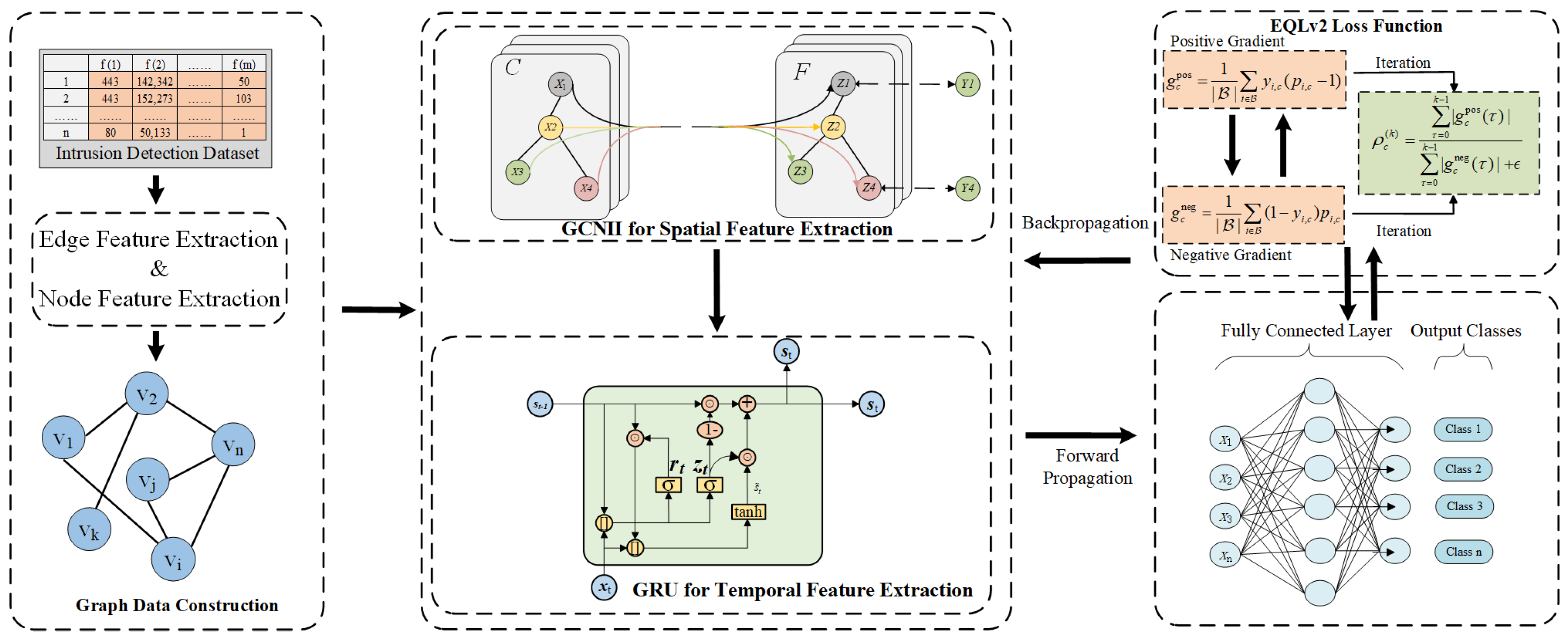
The STEGCN framework amalgamates an enhanced GCN, GRU, and an advanced EQLv2 function into a unified, end-to-end spatio-temporal graph-based intrusion detection model. As conceptually illustrated in Figure 1, the architecture is composed of three interconnected modules. These modules include, firstly, the Spatial Feature Extractor, which leverages GCNII to discern multi-scale spatial features for nodes within each temporal graph snapshot, thereby capturing intricate inter-entity associations in the network; secondly, the Temporal Feature Modeler, employing GRU to characterize the temporal dynamics of the spatial feature sequences, thus capturing multi-stage evolutionary patterns of attack behaviors; thirdly, the Balanced Classification Decider, which utilizes the EQLv2 loss function for classification predictions, dynamically equilibrating gradient contributions across classes to address the inherent class imbalance challenge. The subsequent subsections elaborate on the design principles of each module and their respective security semantics within the context of intrusion detection.

3.2.1. GCNII−Based Spatial Feature Extraction

Conventional GCNs are designed to extract spatial node features through symmetric normalized neighborhood aggregation. However, they are inherently susceptible to over-smoothing as network depth increases. As the number of layers grows, node representations from different classes tend to converge, leading to a significant loss of discriminative capability. This issue arises from repeated Laplacian smoothing, which progressively drives node features toward a global mean and suppresses local structural information. In the context of intrusion detection, deep graph architectures are essential for modeling complex attack behaviors. While single-hop aggregation mainly captures directly connected anomalies, multi-hop aggregation is necessary to uncover attack propagation paths and diffusion dynamics, such as worm spreading or lateral movement in multi-stage attacks. To address the over-smoothing limitation, the Graph Convolutional Network with Initial residual and Identity mapping (GCNII) is employed as the spatial feature extractor. By incorporating initial residual connections and adaptive identity mappings, GCNII effectively alleviates over-smoothing and enables stable deep graph representation learning.

For the graph snapshot at time step t, $G^{\left(t\right)}=({\mathcal{V}}^{\left(t\right)},{\mathcal{E}}^{\left(t\right)},{\mathbf{X}}^{\left(t\right)})$, spatial feature extraction is performed using an L-layer GCNII. The symmetric normalization procedure first constructs the adjacency matrix with self-loops $\tilde{\mathbf{A}}={\mathbf{A}}^{\left(t\right)}+\mathbf{I}$, computes the degree matrix $\tilde{\mathbf{D}}$ with diagonal entries ${\tilde{D}}_{ii}={\sum }_{j=1}^{n_t}{\tilde{A}}_{ij}$, and yields the normalized matrix:

$$\tilde{\mathbf{P}}={\tilde{\mathbf{D}}}^{-{\displaystyle \frac{1}{2}}}\tilde{\mathbf{A}}{\tilde{\mathbf{D}}}^{-{\displaystyle \frac{1}{2}}}\in {\mathbb{R}}^{n_t\times n_t}.$$

(9)

The forward propagation at layer $l+1$ ($l=0,1,\dots ,L-1$) is defined as

$$\begin{array}{cc}\hfill {\mathbf{H}}^{(l+1)}& =\sigma \left(\left((1-{\alpha }_l)\tilde{\mathbf{P}}{\mathbf{H}}^{\left(l\right)}+{\alpha }_l{\mathbf{H}}^{\left(0\right)}\right)\left((1-{\beta }_l)\mathbf{I}+{\beta }_l{\mathbf{W}}^{\left(l\right)}\right)\right),\hfill \end{array}$$

(10)

where ${\mathbf{H}}^{\left(0\right)}={\mathbf{X}}^{\left(t\right)}\in {\mathbb{R}}^{n_t\times d^{\prime }}$ is the input feature matrix, ${\mathbf{H}}^{\left(l\right)}\in {\mathbb{R}}^{n_t\times d_h}$ denotes the node representations at layer l ($d_h$ is the hidden dimension), ${\mathbf{W}}^{\left(l\right)}\in {\mathbb{R}}^{d_h\times d_h}$ is the trainable weight matrix at layer l, $\sigma (·)$ is the ReLU activation, and $\mathbf{I}\in {\mathbb{R}}^{d_h\times d_h}$ is the identity matrix. The hyperparameter ${\alpha }_l\in [0,1]$ controls the initial residual strength, governing retention of raw input features; ${\beta }_l=log({\displaystyle \frac{\lambda }{l}}+1)$ ($\lambda >0$ is a hyperparameter) adaptively modulates the identity mapping across layers. In practical applications, the hyperparameters ${\alpha }_l$ and $\lambda$ have a significant impact on the model’s deep representation capability. The parameter ${\alpha }_l$ controls the strength of the initial residual connection. A smaller value of ${\alpha }_l$ (e.g., 0.1) encourages the model to rely more on layer-wise aggregation of neighborhood information, which is more suitable for shallow networks. In contrast, a larger ${\alpha }_l$ (e.g., 0.3–0.5) preserves a greater proportion of the original features, thereby effectively alleviating the over-smoothing problem in deep networks. The parameter $\lambda$ regulates the adaptive decay of the identity mapping through ${\beta }_l$. A larger $\lambda$ allows the shallow layers to focus more on learning representations via parameterized transformations, while the deeper layers gradually approach identity mappings to stabilize the learned representations. Conversely, a smaller $\lambda$ accelerates this transition process.

The initial residual connection establishes direct pathways from the input ${\mathbf{H}}^{\left(0\right)}$ to every intermediate layer, thereby ensuring that deep representations robustly preserve discriminative information originating from raw features. Mathematically, this mechanism counteracts over-smoothing: While standard GCN propagation ${\mathbf{H}}_{\mathrm{std}}^{(l+1)}=\sigma \left(\tilde{\mathbf{P}}{\mathbf{H}}^{\left(l\right)}{\mathbf{W}}^{\left(l\right)}\right)$ causes repeated Laplacian smoothing that drives features toward convergence, the initial residual term ${\alpha }_l{\mathbf{H}}^{\left(0\right)}$ maintains

$${\parallel {\mathbf{H}}^{\left(l\right)}-{\mathbf{H}}^{\left(0\right)}\parallel }_F\le C,\forall l,$$

(11)

where C is a constant bounded by ${\alpha }_l$, ensuring that node representations remain within a bounded distance from the original features regardless of depth. When ${\alpha }_l>0$, the multi-layer propagation effectively retains memory of the initial inputs, which robustly counteracts the over-smoothing phenomenon. Concurrently, the adaptive identity mapping integrates the identity matrix $\mathbf{I}$ into weight transformations, fundamentally preventing performance degradation with increasing network depth. The specific design of ${\beta }_l$ ensures a layer-wise adaptive mechanism: In shallow layers (small l), ${\beta }_l\approx 1$, which prioritizes parameterized transformations via ${\mathbf{W}}^{\left(l\right)}$ to learn highly expressive features; conversely, in deeper layers (large l), ${\beta }_l$ diminishes, thereby strengthening the identity mapping to stabilize the node representations. Specifically, for large l, such as ${\beta }_l\to 0$, the weight transformation approaches

$$(1-{\beta }_l)\mathbf{I}+{\beta }_l{\mathbf{W}}^{\left(l\right)}\approx \mathbf{I},$$

(12)

which prevents gradient vanishing and maintains representation stability. This balanced layer-wise mechanism enables GCNII to effectively harmonize expressive feature learning with representation stability, supporting the efficient training of profoundly deep graph networks.

Following L layers of GCNII, the extracted spatial representation for node i at time t is denoted as ${\mathbf{h}}_i^{\left(t\right)}={\mathbf{H}}^{\left(L\right)}[i,:]\in {\mathbb{R}}^{d_h}$, which aggregates information from its L-hop neighborhood, formally defined as ${\mathcal{N}}_L\left(i\right)=\{j\in {\mathcal{V}}^{\left(t\right)}\mid d_G(i,j)\le L\}$, where $d_G(i,j)$ denotes the shortest path distance between nodes i and j in graph $G^{\left(t\right)}$. These multi-scale spatial features encode security semantics at varying granularities. Single-hop aggregation captures anomalous patterns; for instance, during port scanning, rapid probing across multiple ports on a target host produces irregularities detectable in a single convolutional layer. Multi-hop aggregation reveals attack propagation dynamics—e.g., worm outbreaks show infected nodes progressively infecting their neighbors, forming spatio-temporal cascades identifiable through deep GCNII architectures. By expanding the receptive field to incorporate global structural information, these deeper architectures further detect topology-level anomalies, such as the star-shaped convergence pattern in Distributed Denial-of-Service (DDoS) attacks, where multiple compromised nodes simultaneously target a single victim.

3.2.2. GRU-Based Temporal Feature Modeling

Network attack behaviors frequently exhibit complex evolutionary patterns across the temporal dimension, dependencies that static analysis methods cannot model. Advanced Persistent Threat (APT) attacks, for instance, typically encompass multiple, sequential stages—including reconnaissance, initial compromise, privilege escalation, lateral movement, and data exfiltration. Each stage is characterized by distinct network behavioral signatures, reflecting the attacker’s evolving strategy over time. To model such multi-stage evolution, GRU units are employed to perform temporal modeling on the spatial features extracted by GCNII. GRUs leverage the synergistic action of update and reset gates to capture long-term temporal dependencies, mitigating the vanishing gradient problem in traditional RNNs. Compared to LSTM networks, GRUs utilize a simplified two-gate architecture (versus LSTM’s three gates), resulting in approximately 25% reduction in parameter count. This design affords superior computational efficiency, making GRUs particularly well suited for modeling the extensive temporal dependencies within large-scale network traffic data.

For node i, its spatial features across time steps are assembled into a temporal sequence $\{{\mathbf{h}}_i^{\left(1\right)},{\mathbf{h}}_i^{\left(2\right)},\dots ,{\mathbf{h}}_i^{\left(T\right)}\}$, where ${\mathbf{h}}_i^{\left(t\right)}\in {\mathbb{R}}^{d_h}$ denotes the GCNII-extracted spatial representation at time step t. The GRU recursively processes this sequence, maintaining a hidden state ${\mathbf{s}}_{t-1}\in {\mathbb{R}}^{d_s}$ ($d_s$ is the GRU hidden state dimension) at each time step t, and updates it based on the current input ${\mathbf{x}}_t={\mathbf{h}}_i^{\left(t\right)}$. The computation proceeds as follows:

$$\begin{array}{cc}\hfill {\mathbf{z}}_t& =\sigma ({\mathbf{W}}_z[{\mathbf{s}}_{t-1};{\mathbf{x}}_t]+{\mathbf{b}}_z),\hfill \end{array}$$

(13)

$$\begin{array}{cc}\hfill {\mathbf{r}}_t& =\sigma ({\mathbf{W}}_r[{\mathbf{s}}_{t-1};{\mathbf{x}}_t]+{\mathbf{b}}_r),\hfill \end{array}$$

(14)

$$\begin{array}{cc}\hfill {\tilde{\mathbf{s}}}_t& =tanh({\mathbf{W}}_h[({\mathbf{r}}_t\odot {\mathbf{s}}_{t-1});{\mathbf{x}}_t]+{\mathbf{b}}_h),\hfill \end{array}$$

(15)

$$\begin{array}{cc}\hfill {\mathbf{s}}_t& =(1-{\mathbf{z}}_t)\odot {\mathbf{s}}_{t-1}+{\mathbf{z}}_t\odot {\tilde{\mathbf{s}}}_t,\hfill \end{array}$$

(16)

where ${\mathbf{z}}_t\in {\mathbb{R}}^{d_s}$ is the update gate, controlling the proportion of the previous hidden state that is retained; ${\mathbf{r}}_t\in {\mathbb{R}}^{d_s}$ is the reset gate, determining how much past information to discard when computing the candidate state; ${\tilde{\mathbf{s}}}_t\in {\mathbb{R}}^{d_s}$ is the candidate hidden state, which integrates the current input with selectively retained history; and ${\mathbf{s}}_t\in {\mathbb{R}}^{d_s}$ is the final hidden state, interpolated between the previous state and the candidate via the update gate. Here, $\sigma (·)$ denotes the sigmoid function, $tanh(·)$ denotes the hyperbolic tangent, $[·;·]$ represents vector concatenation, and ⊙ denotes the Hadamard (element-wise) product. The trainable parameters are ${\mathbf{W}}_z,{\mathbf{W}}_r,{\mathbf{W}}_h\in {\mathbb{R}}^{d_s\times (d_s+d_h)}$ and ${\mathbf{b}}_z,{\mathbf{b}}_r,{\mathbf{b}}_h\in {\mathbb{R}}^{d_s}$.

The GRU module models the time series of node features. By successively accumulating temporal features across the window, the hidden state ${\mathbf{s}}_t$ from each unit carries historical sequential information, which is passed to the next processing unit. The final state, ${\mathbf{s}}_T$, therefore serves as the comprehensive spatio-temporal representation for node i, effectively encoding the evolutionary dynamics across the entire time window.

3.2.3. EQLv2-Based Balanced Classification Decision

The class imbalance problem in intrusion detection is characterized by extreme skewness and a long-tail distribution. Benign traffic typically constitutes over $95\%$ of total flows, with malicious traffic below $5\%$, leading to severe class imbalance. Furthermore, sample counts vary drastically across attack types, forming a classic long-tail distribution where high-risk attacks (e.g., zero-day exploits, APTs) are extremely rare compared to common ones (e.g., denial-of-service). Under standard cross-entropy loss ${\mathcal{L}}_{\mathrm{CE}}=-{\displaystyle \frac{1}{N}}{\sum }_{i=1}^N{\sum }_{c=0}^{C-1}{y}_{i,c}log\left(p_{i,c}\right)$, the gradient magnitude for class c is proportional to its sample count:

$$∥{\displaystyle \frac{\partial {\mathcal{L}}_{\mathrm{CE}}}{\partial {\mathbf{W}}_c}}∥\propto N_c,$$

(17)

where $N_c={\sum }_{i=1}^N{y}_{i,c}$ is the number of samples in class c, and ${\mathbf{W}}_c$ denotes the classifier parameters for class c. This causes the benign class ($c=0$) to potentially contribute tens or hundreds of times more gradient than rare attack classes, resulting in late-stage overfitting and critical underperformance on minorities.

To circumvent this issue, EQLv2 is adopted as the training objective. EQLv2 balances gradient contributions across classes via a dynamic gradient steering mechanism: It monitors the cumulative positive-to-negative gradient ratio for each classifier and adaptively adjusts gradient weights to ensure comparable update magnitudes across all classes. Unlike Focal Loss, which reweights samples based on prediction confidence, EQLv2 balances learning progress by training difficulty rather than sample frequency, reducing overfitting risk on rare classes.

For a C-class problem, the classification output layer comprises C independent classifiers. A fully connected layer maps the spatio-temporal feature ${\mathbf{s}}_i$ to class logits:

$${\mathbf{z}}_i={\mathbf{W}}_{\mathrm{cls}}{\mathbf{s}}_i+{\mathbf{b}}_{\mathrm{cls}},$$

(18)

where ${\mathbf{z}}_i\in {\mathbb{R}}^C$ is the logit vector, and ${\mathbf{W}}_{\mathrm{cls}}\in {\mathbb{R}}^{C\times d_s}$, ${\mathbf{b}}_{\mathrm{cls}}\in {\mathbb{R}}^C$ are the classifier parameters. After softmax normalization, the probability distribution is ${\mathbf{p}}_i=\mathrm{softmax}\left({\mathbf{z}}_i\right)$, with $p_{i,c}={\displaystyle \frac{exp\left(z_{i,c}\right)}{{\sum }_{j=0}^{C-1}exp\left(z_{i,j}\right)}}$. For classifier c, the positive and negative gradients over the current batch $\mathcal{B}$ are rigorously defined as

$$g_c^{\mathrm{pos}}={\displaystyle \frac{1}{\left|\mathcal{B}\right|}}\sum _{i\in \mathcal{B}}{y}_{i,c}(p_{i,c}-1),g_c^{\mathrm{neg}}={\displaystyle \frac{1}{\left|\mathcal{B}\right|}}\sum _{i\in \mathcal{B}}(1-y_{i,c})p_{i,c},$$

(19)

where $y_{i,c}\in \{0,1\}$ is the one-hot label ($y_{i,c}=1$ if sample i belongs to class c), and $p_{i,c}$ is the predicted probability.

EQLv2 maintains a cumulative gradient tracker and computes the gradient ratio ${\rho }_c^{\left(k\right)}$ at training iteration k as the ratio of cumulative absolute positive-to-negative gradients for class c:

$${\rho }_c^{\left(k\right)}={\displaystyle \frac{{\sum }_{\tau =0}^{k-1}\left|g_c^{\mathrm{pos}}\left(\tau \right)\right|}{{\sum }_{\tau =0}^{k-1}\left|g_c^{\mathrm{neg}}\left(\tau \right)\right|+ϵ}},$$

(20)

where $ϵ={10}^{-8}$ ensures numerical stability. It is then mapped to the dynamic weight coefficients $w_c^{\mathrm{pos},\left(k\right)}$ and $w_c^{\mathrm{neg},\left(k\right)}$ via a sigmoid function $\varphi (x;\gamma ,\mu )={\displaystyle \frac{1}{1+exp(-\gamma (x-\mu \left)\right)}}$:

$$w_c^{\mathrm{pos},\left(k\right)}=1+\alpha (1-\varphi ({\rho }_c^{\left(k\right)};\gamma ,\mu )),w_c^{\mathrm{neg},\left(k\right)}=\varphi ({\rho }_c^{\left(k\right)};\gamma ,\mu ),$$

(21)

where $\gamma >0$ controls the sigmoid steepness, $\mu >0$ (typically $\mu =1$) is the center offset, and $\alpha >0$ controls the adjustment strength. This design creates a feedback mechanism:

$$\mathrm{If}{\rho }_c^{\left(k\right)}\gg 1:w_c^{\mathrm{neg},\left(k\right)}\to 1,\mathrm{If}{\rho }_c^{\left(k\right)}\ll 1:w_c^{\mathrm{pos},\left(k\right)}\to 1+\alpha ,$$

(22)

which amplifies negative updates when positive gradients dominate and vice versa.

Furthermore, to ensure sufficient updates for extremely rare classes, EQLv2 introduces a frequency threshold $\tau \in (0,1)$, partitioning classes into frequent ($f_c={\displaystyle \frac{N_c}{N}}\ge \tau$) and rare ($f_c<\tau$), where $f_c$ denotes the class frequency. Rare classes are exempt from gradient suppression (${\nu }_c=1$). For frequent classes, a gradient-guided suppression weight ${\nu }_c$ is computed:

$${\nu }_c=\left\{\begin{array}{cc}1,\hfill & \mathrm{if}{f}_c<\tau (\mathrm{rare}\mathrm{class}),\hfill \\ 1-\beta ·{\mathbb{E}}_{j\in {\mathcal{C}}_{\mathrm{freq}}}\left[\max (0,g_j^{\mathrm{pos}})\right],\hfill & \mathrm{if}{f}_c\ge \tau (\mathrm{frequent}\mathrm{class}),\hfill \end{array}\right.$$

(23)

where ${\mathcal{C}}_{\mathrm{freq}}=\{c\mid f_c\ge \tau \}$ is the frequent class set, and $\beta \in (0,1)$ is the suppression strength. This mechanism reduces the loss weight of a frequent class when other frequent classes exhibit high positive gradients, effectively curbing their dominance and reallocating optimization capacity toward rare classes. The final EQLv2 loss is formulated as

$${\mathcal{L}}_{\mathrm{EQL}}=-{\displaystyle \frac{1}{N}}\sum _{i=1}^N\sum _{c=0}^{C-1}{\nu }_c·y_{i,c}log\left(p_{i,c}\right),$$

(24)

where ${\nu }_c$ is dynamically computed, ensuring that rare classes ($f_c<\tau$) maintain full gradient updates while frequent classes are adaptively suppressed based on peer gradient activity.

3.2.4. Overall Training Objective and Enhancement Strategies

The overall objective function utilized for training the STEGCN model is a composite loss, comprising three distinct components:

$${\mathcal{L}}_{\mathrm{total}}={\mathcal{L}}_{\mathrm{EQL}}+{\lambda }_1{\mathcal{L}}_{\mathrm{reg}}+{\lambda }_2{\mathcal{L}}_{\mathrm{graph}},$$

(25)

where ${\mathcal{L}}_{\mathrm{EQL}}$ is the EQLv2 classification loss, specifically designed to mitigate class imbalance. The parameter regularization term, ${\mathcal{L}}_{\mathrm{reg}}=\parallel {\mathsf{\Theta }}_{\mathrm{GCNII}}{\parallel }_2^2+\parallel {\mathsf{\Theta }}_{\mathrm{GRU}}{\parallel }_2^2+{\parallel {\mathsf{\Theta }}_{\mathrm{cls}}\parallel }_2^2$, imposes ${\mathcal{\ell }}_2$ constraints on all trainable parameters ($\mathsf{\Theta }$) to curb overfitting and enhance generalization. ${\mathsf{\Theta }}_{\mathrm{GCNII}}$, ${\mathsf{\Theta }}_{\mathrm{GRU}}$, and ${\mathsf{\Theta }}_{\mathrm{cls}}$ denote the parameter sets of the GCNII, GRU, and classifier modules, respectively. The graph structure regularization loss is defined as

$${\mathcal{L}}_{\mathrm{graph}}={\displaystyle \frac{1}{2{\sum }_{t=1}^T\left|{\mathcal{E}}^{\left(t\right)}\right|}}\sum _{t=1}^T\sum _{(i,j)\in {\mathcal{E}}^{\left(t\right)}}{\parallel {\mathbf{s}}_i-{\mathbf{s}}_j\parallel }_2^2.$$

(26)

This term enforces consistency between the final spatio-temporal representations (${\mathbf{s}}_i,{\mathbf{s}}_j$) of connected nodes. It is mathematically grounded in the graph smoothness assumption: If nodes i and j are directly linked, i.e., $(i,j)\in {\mathcal{E}}^{\left(t\right)}$, minimizing this term forces their final representations to be similar, thereby reinforcing the model’s exploitation of the inherent graph topology. The hyperparameters ${\lambda }_1,{\lambda }_2>0$ control the weighting of each regularization term and are determined empirically via validation performance.

To further enhance detection performance and adaptability, two augmentation strategies are integrated. The first addresses performance fluctuations across attack timescales, stemming from a fixed window T being inadequate for capturing multi-scale temporal dynamics (short-burst attacks vs. long-latency APTs). To mitigate this, a multi-scale temporal modeling strategy employs multiple window lengths $\{T_1,T_2,\dots ,T_M\}$ to model short-, medium-, and long-term dependencies. For each scale m, an independent GRU module ${\mathrm{GRU}}_m$ processes a sequence of length $T_m$ to yield ${\mathbf{s}}_i^{\left(m\right)}$. A self-attention mechanism then adaptively fuses this information using dynamically computed scale importance weights ${\alpha }_m$:

$${\mathbf{s}}_i^{\left(m\right)}={\mathrm{GRU}}_m(\{{\mathbf{h}}_i^{(t-T_m+1)},\dots ,{\mathbf{h}}_i^{\left(t\right)}\};{\mathsf{\Theta }}_{\mathrm{GRU}}^{\left(m\right)})\in {\mathbb{R}}^{d_s},$$

(27)

$${\alpha }_m={\displaystyle \frac{exp\left({\mathbf{w}}_m^T{\mathbf{s}}_i^{\left(m\right)}\right)}{{\sum }_{j=1}^{M}exp\left({\mathbf{w}}_j^T{\mathbf{s}}_i^{\left(j\right)}\right)}},{\mathbf{s}}_i=\sum _{m=1}^M{\alpha }_m{\mathbf{s}}_i^{\left(m\right)}.$$

(28)

The resulting ${\mathbf{s}}_i$ autonomously prioritizes the most relevant timescale (e.g., $T_1$ for port scanning, $T_3$ for long-cycle APTs).

The second strategy, adaptive graph learning, overcomes the limitations of rule-based graph construction by dynamically refining the graph structure to uncover data-driven latent associations. The final adjacency matrix ${\mathbf{A}}^{\left(t\right)}$ is defined as a convex combination of the initial rule-based matrix ${\mathbf{A}}_0^{\left(t\right)}$ and the learned adaptive matrix ${\mathbf{A}}_{\mathrm{adapt}}^{\left(t\right)}$:

$${\mathbf{A}}^{\left(t\right)}=(1-\gamma ){\mathbf{A}}_0^{\left(t\right)}+\gamma {\mathbf{A}}_{\mathrm{adapt}}^{\left(t\right)},$$

(29)

where $\gamma \in [0,1]$ balances the structures. The adaptive adjacency $A_{\mathrm{adapt},ij}^{\left(t\right)}$ is derived from node feature similarity, $s_{ij}=\sigma \left({\mathbf{h}}_i^T{\mathbf{W}}_{\mathrm{sim}}{\mathbf{h}}_j\right)$, employing a top-K sparsification strategy to ensure computational efficiency:

$$A_{\mathrm{adapt},ij}^{\left(t\right)}=\left\{\begin{array}{cc}\sigma \left({\mathbf{h}}_i^T{\mathbf{W}}_{\mathrm{sim}}{\mathbf{h}}_j\right)\hfill & \mathrm{if}j\in {\mathcal{N}}_K\left(i\right),\hfill \\ 0\hfill & \mathrm{otherwise},\hfill \end{array}\right.$$

(30)

where ${\mathcal{N}}_K\left(i\right)$ represents the set of top-K neighbors of node i by similarity. This enables the discovery of associations missed by predefined rules (e.g., linking flows via statistical feature similarity).

From a computational perspective, STEGCN’s overall time complexity is $O\left(TL\right|\mathcal{E}|d_h+nT{d}_s^2+nC{d}_s)$. Under sparse graphs ($\left|\mathcal{E}\right|=O\left(n\right)$), complexity simplifies to $O(TLn{d}_h+nT{d}_s^2+nC{d}_s)$. This demonstrates significant efficiency compared to fully connected networks $O\left(n{d}^{\prime 2}L\right)$. Relative to a standard GCN+LSTM architecture, replacing the LSTM unit with GRU reduces the total number of temporal parameters by approximately $25\%$ (specifically, from $4(d_s^2+d_s{d}_h)$ parameters to $3(d_s^2+d_s{d}_h)$ parameters), inherently enhancing training efficiency. Through graph sparsity and parameter sharing, STEGCN achieves substantial computational efficiency while preserving expressive power, making it suitable for real-time detection in large-scale network traffic.

In summary, STEGCN delivers a technically advanced solution for network intrusion detection via deep integration of graph neural networks and recurrent neural networks, augmented by a state-of-the-art balanced loss design, multi-scale temporal modeling, and adaptive graph learning. The model not only effectively extracts spatio-temporal features from network traffic but also robustly handles class imbalance, achieving precise identification of complex attack patterns with high computational efficiency.

4. Experiment and Result Analysis

4.1. Experiment Environment

Table 1. Experimental hardware and software specifications.

Component	Specification
Operating System	Windows 11 (Microsoft Corporation, Redmond, WA, USA)
CPU	Intel(R) Core(TM) i7-11700 (Intel Corporation, Santa Clara, CA, USA)
GPU	NVIDIA GeForce RTX 3060 (NVIDIA Corporation, Santa Clara, CA, USA)
RAM	32 GB
Python	3.8.3 (Python Software Foundation, Wilmington, DE, USA)
Deep Learning Framework	PyTorch 2.1.0 (Meta Platforms Inc., Menlo Park, CA, USA)
Graph Neural Network Library	PyTorch Geometric 2.4.0 (https://pytorch-geometric.readthedocs.io)

presents the experimental hardware and software specifications.

4.2. Datasets and Data Processing

To validate the effectiveness and generalization capability of the proposed model, this study selected two widely recognized network security benchmark datasets: CICIDS2017 and UNSW-NB15. These two datasets exhibit complementarity in terms of network traffic characteristics, attack type coverage, and data scale, enabling comprehensive evaluation of intrusion detection model performance across different network environments.

The CICIDS2017 dataset, published by the Canadian Institute for Cybersecurity, is specifically designed for Network Intrusion Detection System (NIDS) research and evaluation [8]. It simulates real-world network traffic patterns, containing both normal and malicious activities. The dataset construction is based on realistic network environments, encompassing network behaviors generated by 25 users through mainstream application protocols. Raw data is recorded in PCAP (Packet Capture) format and processed by the CICFlowMeter tool to extract key network features such as timestamps, IP addresses, port numbers, and protocol types into CSV format.

To address the class imbalance in the original dataset, this study adopted preprocessing strategies from existing CICIDS2017 research [22]. Specifically, attack categories were relabeled and regrouped based on attack behavior similarity. Given that attack types such as DoS GoldenEye, DoS Hulk, DoS Slowloris, Heartbleed, DoS Slowhttptest, and DDoS exhibit high similarity in attack mechanisms and network behavioral characteristics, this study unified them into the “DoS/DDoS” category. Meanwhile, the Infiltration category contained only 36 samples, severely insufficient for model training and was excluded. After regrouping, the dataset contains 6 categories, with distributions shown in

Table 2. Class distribution of the CICIDS2017 dataset after relabeling.

New Label	Original Label	Quantity
Benign	Benign	2,271,320
DoS/DDoS	DDoS DoS GoldenEye DoS Hulk DoS Slowhttptest DoS Slowloris Heartbleed	379,748
PortScan	PortScan	158,804
Brute Force	FTP-Patator SSH-Patator	13,832
Web Attack	Brute Force SQL Injection XSS	2180
Botnet	Bot	1956

.

The UNSW-NB15 dataset was developed by the Cyber Security Research Center at the University of New South Wales [23] and represents a widely recognized benchmark dataset in network security. The dataset construction employed rigorous experimental design: the research team utilized IXIA PerfectStorm professional network testing equipment to establish a controlled experimental environment, simulating realistic network scenarios through carefully designed network topology. The experimental network architecture comprises three dedicated servers, where servers 1 and 3 generate normal traffic, and server 2 produces attack traffic. The entire test network is interconnected through a dual-router architecture (primary router and backup router), ensuring comprehensive and reliable data collection. A total of 100GB of raw network packets (PCAP format) were collected.

Based on professional network analysis tools such as Argus and Bro-IDS, researchers developed 12 feature extraction algorithms, constructing a standardized dataset with 49 feature dimensions (including class labels). This dataset integrates normal traffic and 9 attack categories, totaling approximately 2.57 million records stored in 4 independent CSV files. The sample distribution of each category is shown in

Table 3. Class quantity distribution of the UNSW-NB15 dataset.

Index	Category	Quantity
0	Benign	22,188,764
1	Generic	215,481
2	Exploits	44,525
3	Fuzzers	14,430
4	DoS	24,246
5	Reconnaissance	13,987
6	Analysis	2677
7	Backdoors	2329
8	Shellcode	1511
9	Worms	174

, reflecting the relative frequency characteristics of different attack types in real network environments.

Following the temporal graph construction described in Section 3.1, network flow records are segmented into non-overlapping time windows according to their timestamps. The window length is set to ${\mathsf{\Delta }}_t=60$ s, providing a trade-off between capturing multi-stage attack dynamics—typically evolving over tens of seconds to minutes—and computational efficiency. Each time window is represented as a graph snapshot, yielding a sequence of temporal graphs.

To reflect realistic intrusion detection deployment and avoid temporal information leakage, the temporal graph sequence is split strictly chronologically: the first 80% of time windows for training and the remaining 20% for testing. This ensures the model is trained solely on historical traffic and evaluated on temporally future data, thereby assessing its generalization to emerging attack patterns. In contrast, random splitting would mix temporally adjacent samples across sets, causing information leakage and overly optimistic performance estimates.

For CICIDS2017, which spans multiple days of traffic collection, the chronological split naturally assigns earlier-day traffic to training and later-day traffic to testing. For UNSW-NB15, the same strategy is applied across all four CSV files based on global timestamp ordering. This temporal partitioning ensures the evaluation accurately reflects the model’s predictive performance in real-world operational settings.

4.3. Evaluation Criteria

Deep learning-based network intrusion detection systems primarily utilize metrics such as accuracy and recall to assess system performance. Here, TP denotes malicious data samples that are correctly identified as attack behaviors, FP represents normal traffic data that are misclassified as attacks, TN refers to data correctly categorized as normal traffic, and FN indicates attack data that are erroneously classified as normal traffic.

Accuracy represents the proportion of samples correctly classified by the model relative to the total number of samples, with its expression given by

$$Accuracy={\displaystyle \frac{TP+TN}{TP+TN+FP+FN}}.$$

(31)

Recall indicates the proportion of positive samples that are correctly predicted, also known as True Positive Rate (TPR):

$$Recall=TPR={\displaystyle \frac{TP}{TP+FN}}.$$

(32)

The F1-score is the harmonic mean of precision and recall, providing a balanced measure of the model’s performance on positive class identification, with its expression denoted as

$$F1=2\times {\displaystyle \frac{TP}{2TP+FP+FN}}.$$

(33)

Conversely, the False Positive Rate (FPR) measures the proportion of normal traffic incorrectly classified as attacks:

$$FPR={\displaystyle \frac{FP}{FP+TN}}.$$

(34)

The area under the ROC curve (AUC) quantifies the model’s ability to distinguish between normal and malicious traffic:

$$AUC=AUC(FPR,TPR).$$

(35)

4.4. Experiments and Results

4.4.1. Comparative Model Performance Analysis

For the hyperparameter configuration of the GCNII component in the proposed model, we follow the recommended settings from [24], adopting ${\alpha }_l=0.1$ and $\lambda =1.0$, with the network depth set to $L=16$. Regarding the feature partition strategy for graph construction, we designate communication relationship features (source/destination IP addresses, source/destination ports, and protocol type) as edge features ${\mathcal{F}}_e$ for defining graph topology, while traffic statistical features (e.g., packet counts, byte volumes, flow duration) serve as node features ${\mathcal{F}}_v$ for characterizing flow behavior. Based on this configuration, this paper compares the performance of the STEGCN model with other traditional machine learning models and deep learning models on two datasets, with the results presented in

Table 4. Performance comparison of different models on the UNSW-NB15 and CICIDS2017 datasets.

Model	UNSW-NB15			CICIDS2017
	Accuracy (%)	Recall (%)	F1 (%)	Accuracy (%)	Recall (%)	F1 (%)
NB	96.0	38.1	52.8	80.1	91.1	85.2
DT	98.1	40.5	55.3	98.5	64.8	76.9
RF	98.1	35.8	51.2	98.5	56.3	70.4
LR	97.5	24.4	38.6	98.5	62.2	75.3
MLP	97.9	37.2	52.5	99.6	76.1	85.7
CNN	97.9	41.7	56.8	99.7	86.2	92.1
RNN	98.0	42.9	58.1	99.7	72.0	83.2
LSTM	98.2	40.5	55.6	99.7	72.7	83.7
GRU	98.0	42.6	57.7	99.7	72.3	83.4
GCN	94.7	51.7	63.5	93.2	98.2	95.6
STEGCN	96.3	66.4	78.6	98.8	99.6	99.2

.

On the UNSW-NB15 dataset, STEGCN achieved an accuracy of 96.3%, a recall of 66.4%, and an F1-score of 78.6%. Despite slightly lower accuracy than traditional models (DT, RF, LR), STEGCN substantially outperformed them in recall (40.5%, 35.8%, 24.4%) and F1-score (55.3%, 51.2%, 38.6%), revealing their limitations in handling class imbalance and rare attacks. STEGCN also surpassed GCN (recall: 51.7%, F1: 63.5%) and time-series models like LSTM and GRU. By integrating spatio-temporal features through the fusion of GCN and GRU, STEGCN demonstrates its distinctive advantage in effectively identifying long-term dependencies in attack behaviors.

On the CICIDS2017 dataset, STEGCN delivered strong results, achieving an accuracy of 98.8%, a recall of 99.6%, and an F1-score of 99.2%. Compared to GCN (recall: 98.2%, F1: 95.6%), STEGCN improved recall by 1.4% and F1-score by 3.6%, demonstrating superior capability in capturing attack patterns and enabling more precise detection of sophisticated threats. Furthermore, STEGCN’s performance significantly exceeds established deep learning models: CNN (recall: 86.2%, F1: 92.1%), RNN ($72.0\%$, 83.2%), LSTM ($72.7\%$, 83.7%), and GRU ($72.3\%$, 83.4%), highlighting its enhanced robustness across diverse attack types. The model sustains this high detection capability even under class imbalance, confirming its advantages for deployment in complex, real-world network environments.

4.4.2. Comparative Analysis of Recall Performance Across Categories

A categorical performance analysis was conducted to benchmark STEGCN against established baselines. As detailed in

Table 5. Recall performance of different models on various categories in the UNSW-NB15 dataset.

Category	Model (Recall%)
	NB	DT	RF	MLP	CNN	RNN	LSTM	GRU	GCN	STEGCN
Benign	98.0	99.0	99.0	99.8	99.6	99.4	99.8	100	98.1	98.6
Generic	2.5	39.5	29.0	38.9	33.7	45.5	25.3	0	97.2	97.3
Exploits	95.0	86.9	89.0	90.4	86.9	84.0	88.6	100	17.1	44.0
Fuzzers	29.9	19.6	21.4	0.4	32.7	65.8	33.8	0	37.5	75.7
DoS	1.4	0	0.7	0	0.6	0	0.9	0	2.5	7.3
Reconnaissance	1.1	73.7	81.8	68.5	59.2	54.9	72.6	100	0	50.9
Analysis	72.3	0	0	0	27.9	0	0	0	86.1	69.7
Backdoors	15.0	1.2	3.7	0	0.6	0	2.4	0	98.6	75.5
Shellcode	66.0	84.2	33.1	74.1	76.4	79.4	82.1	100	4.1	48.3
Worms	0	0	0	0	0	0	0	0	76.3	76.3

, on the UNSW-NB15 dataset, STEGCN recorded an aggregate recall of $66.4\%$, representing a marked improvement over GCN’s $51.7\%$ baseline, as well as outperforming both traditional machine learning algorithms (e.g., DT, RF) and standard deep learning architectures (e.g., CNN, RNN). STEGCN excels in the Generic and Fuzzers categories, yielding recall rates of $97.3\%$ and $75.7\%$, respectively—metrics that substantially eclipse those of competing models. For the Backdoors category, STEGCN achieved a recall of $75.5\%$; while this ranks second to GCN ($98.6\%$), it represents a dramatic advantage over the negligible detection rates observed in RF ($3.7\%$) and CNN ($0.6\%$).

STEGCN achieved recall rates of $44\%$ and $48.3\%$ for the Exploits and Shellcode categories, respectively, showing notable improvement over GCN ($17.1\%$ and $4.1\%$). This indicates that STEGCN possesses advantages over traditional graph neural networks in extracting spatio-temporal attack features. For DoS attacks, STEGCN achieved $7.3\%$, higher than GCN’s $2.5\%$, but remains relatively low, suggesting the need for further optimization for this attack type.

In summary, STEGCN demonstrates superior detection capabilities on UNSW-NB15, particularly in addressing class imbalance, though optimization opportunities remain for DoS and Exploits categories.

On the CICIDS2017 dataset, as shown in

Table 6. Recall performance of different models on various categories in the the CICIDS2017 Dataset.

Category	Model (Recall%)
	NB	DT	RF	MLP	CNN	RNN	LSTM	GRU	GCN	STEGCN
Benign	78.2	99.5	99.8	99.8	99.8	99.9	99.3	100	92.3	98.5
DoS/DDoS	88.4	94.1	92.7	99.1	99.6	99.6	99.2	100	97.6	99.9
PortScan	97.4	94.6	97.4	99.4	99.6	99.7	99.7	100	99.4	99.9
Brute Force	98.5	98.1	46.6	98.3	98.5	99.2	99.3	100	100	100
Web Attack	85.7	0	0	0	93.6	4.2	5.1	0	100	99.5
Botnet	98.7	0	1.4	59.7	26.2	29.6	32.2	0	100	100

, STEGCN achieved an overall recall of $99.6\%$, outperforming GCN’s $98.2\%$ and all other baselines. For the Benign traffic category, STEGCN attained a recall of $98.5\%$, significant improvement over GCN’s $92.3\%$. In the DoS/DDoS and PortScan categories, STEGCN achieved recall rates of $99.9\%$ for both, surpassing GCN and traditional methods, demonstrating its strong performance for large-scale traffic attacks and port scanning. For the Brute Force and Botnet categories, STEGCN achieved perfect recall rates of $100\%$, substantially outperforming RF and DT, confirming the advantages of graph-based modeling in detecting brute force attacks and botnet.

For the Web Attack category, STEGCN achieved a recall of $99.5\%$, exceeding conventional methods such as CNN ($93.6\%$) and MLP ($0\%$). Notably, GCN attained a $100\%$ recall in this category, evidencing the efficacy of graph neural networks in capturing web attack patterns. Leveraging this architectural advantage, STEGCN maintained comparable high-level performance. In summary, on the CICIDS2017 dataset, STEGCN demonstrates superior detection capability over both traditional and deep learning baselines, yielding optimal or near-optimal recall rates across the majority of attack categories.

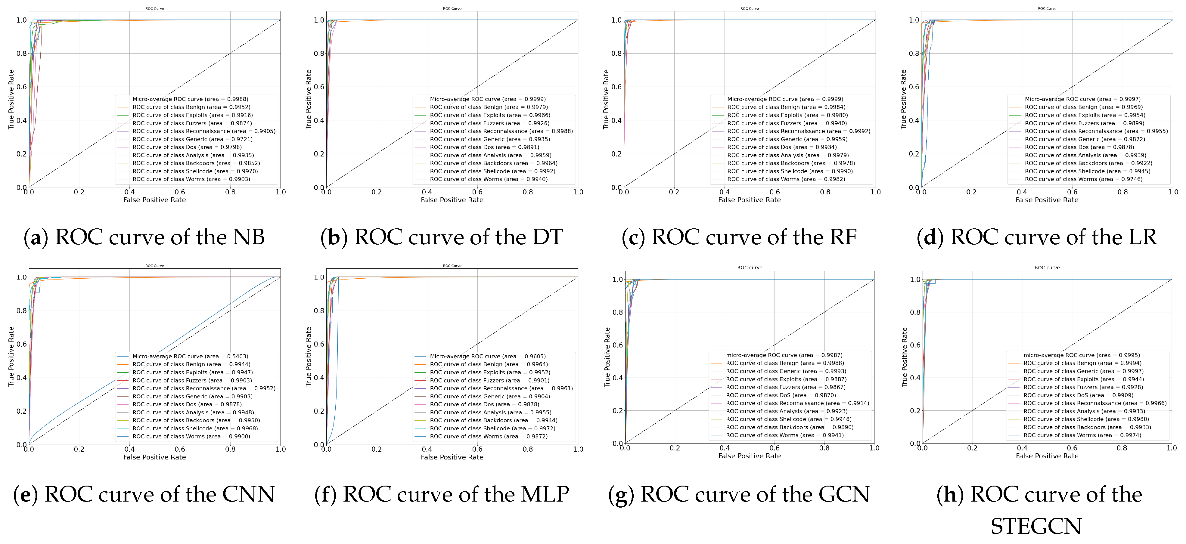
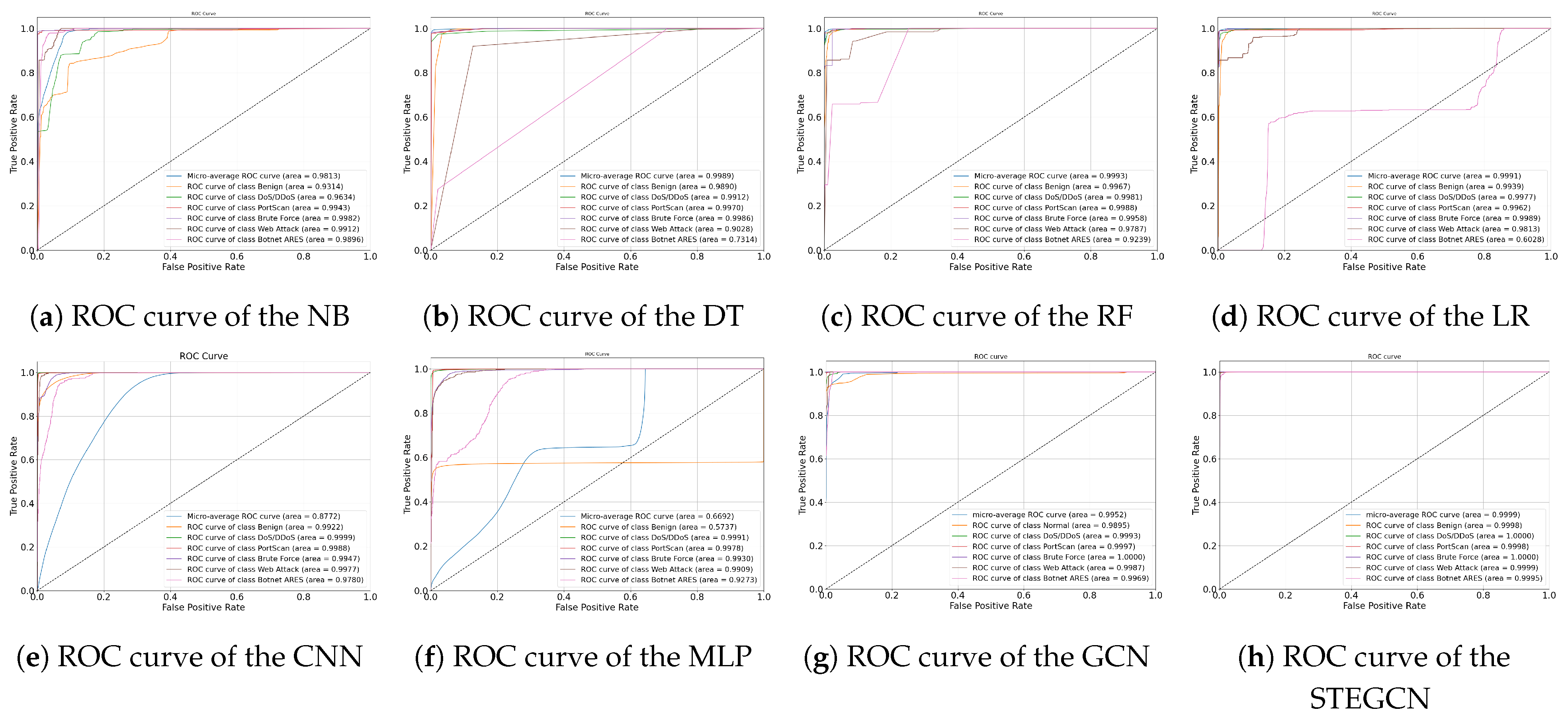
Figure 2 and Figure 3 present the ROC curves comparing different models on the UNSW-NB15 and CIC-IDS2017 datasets, respectively. On the UNSW-NB15 dataset, STEGCN achieves a micro-average AUC of 0.9995, which is comparable to that of DT and RF, and superior to the other baseline models. In contrast, CNN and MLP exhibit noticeably weaker overall classification performance. Regarding per-class detection performance, STEGCN demonstrates a clear advantage on minority attack classes, particularly maintaining high AUC values for extremely rare classes such as Shellcode and Worms, whereas traditional machine learning models show evident limitations and performance gaps on these categories. This highlights their restricted capability in addressing severe class imbalance.

The experimental results on the CIC-IDS2017 dataset further corroborate the above findings. STEGCN attains an impressive micro-average AUC of 0.9999, achieving perfect scores (AUC = 1.0000) on both DoS/DDoS and Brute Force categories. By comparison, several baseline models perform poorly on specific attack types; for instance, DT and LR yield AUC values below 0.75 on the Botnet ARES class.

In summary, by effectively integrating temporal feature extraction with a gradient-balancing mechanism, STEGCN consistently delivers stable and superior detection performance across diverse datasets and attack types, particularly excelling in handling class imbalance and minority/rare attack classes in network intrusion detection tasks.

4.4.3. Comparative Performance Analysis of Existing Methods

Multi-classification performance was benchmarked against various existing methodologies on the UNSW-NB15 and CICIDS2017 datasets. On the UNSW-NB15 dataset (detailed in

Table 7. Performance comparison in the UNSW-NB15 dataset.

Model	Accuracy (%)	Recall (%)	F1 (%)
Proposed Model	96.3	66.4	78.6
CNN [25]	93.82	37.50	52.4
KNN [26]	97.36	60.50	73.8
DT [26]	97.19	60.7	73.9
LR [26]	95.12	49.4	63.2
SVM [27]	98.0	61.7	75.2
XGB [28]	83.2	65.3	72.8
AdaBoost [28]	57.5	40.1	46.3
MLP [28]	80.1	48.5	59.6
1-D CNN [29]	76.3	76.1	76.2
CNN-BiLSTM [30]	82.0	48.0	59.8

), STEGCN achieved an overall classification accuracy of 96.3%, a recall of 66.4%, and an F1-score of 78.6%. While traditional classifiers, including KNN (Acc $97.36\%$, Rec $60.5\%$, F1 $73.8\%$), DT (Acc $97.19\%$, Rec $60.7\%$, F1 $73.9\%$), and SVM (Acc $98.0\%$, Rec $61.7\%$, F1 $75.2\%$), exhibited marginally higher accuracy, STEGCN registered a superior recall gain of approximately $5.5\%$ and F1-score improvement of approximately $3.4\%$. This strategic trade-off confirms STEGCN’s explicit design advantage in minority-class attack detection, demonstrating its capability to identify attack samples more comprehensively while effectively managing the False Positive rate.

Against deep learning architectures, STEGCN outperformed CNN, MLP, and CNN-BiLSTM in all metrics. Compared to 1-D CNN (Acc $76.3\%$, Rec $76.1\%$, F1 $76.2\%$), although STEGCN showed marginally lower recall, it achieved substantially higher accuracy (+20%) and F1-score (+2.4%), validating its superior ability to control misclassification while maintaining high detection efficacy.

The comparison with XGB is particularly noteworthy: while XGB achieved a recall of $65.3\%$ (approaching STEGCN’s $66.4\%$) and F1-score of $72.8\%$, its accuracy was limited to $83.2\%$, substantially lower than STEGCN’s. This disparity highlights STEGCN’s strategic advantage in significantly improving accuracy (+13.1%) and F1-score (+5.8%) while sustaining high recall, confirming its superior efficacy in overall performance.

For the CICIDS2017 dataset (

Table 8. Performance comparison in the CICIDS2017 dataset.

Model	Accuracy (%)	Recall (%)	F1 (%)
Proposed Model	98.7	99.6	99.2
DNN [31]	94.6	84.6	89.2
LSTM [32]	98.9	74.8	85.0
TBLS(W) [33]	97.8	97.0	97.4
MFFSEN(W) [34]	99.9	99.9	99.9
MECNN [35]	99.7	79.1	87.9
MBGAN [10]	94.8	96.5	95.6
SE-MBL [11]	93.9	94.89	94.4

), STEGCN achieved highly competitive multi-classification performance with an accuracy of 98.7%, a recall of 99.6%, and an F1-score of 99.2%. Models such as SE-MBL (Acc $93.9\%$, Rec $94.89\%$, F1 $94.4\%$) and TBLS(W) (Acc $97.8\%$, Rec $97.0\%$, F1 $97.4\%$) showed strong performance but remained quantitatively inferior to STEGCN. Similarly, the LSTM model (Acc $98.9\%$, Rec $74.8\%$, F1 $85.0\%$) yielded comparable accuracy but significantly underperformed in recall and F1-score. We note that MFFSEN(W) reported near-perfect metrics (Acc $99.9\%$, Rec $99.9\%$, F1 $99.9\%$), slightly exceeding STEGCN; however, this result is limited by its use of only Wednesday’s data from the CICIDS2017 dataset during training and testing, presenting an inherent methodological constraint. Conversely, MECNN reported a $1\%$ higher accuracy than STEGCN but failed to achieve $80\%$ recall (Rec $79.1\%$, F1 $87.9\%$), strongly indicating a significant deficiency in identifying true attack samples.

These comparative results confirm that while certain methods exhibit comparable or marginally superior performance on specific, isolated metrics, the STEGCN model provides a superior comprehensive detection capability. Its achieved performance across accuracy, recall, and F1-score consistently meets or surpasses the performance of the majority of existing benchmarks.

4.4.4. Ablation Study

To validate the effectiveness of each component in STEGCN, we conduct ablation experiments on the UNSW-NB15 and CICIDS2017 datasets. Using GCNII as the baseline model, we progressively incorporate the GRU module and EQLv2 loss function to analyze the contribution of each component. The results are presented in

Table 9. Ablation study results from the UNSW-NB15 and CICIDS2017 datasets.

Dataset	Model	Accuracy (%)	Recall (%)	F1 (%)
UNSW-NB15	GCNII	93.9	45.3	57.2
	+GRU	95.8	53.2	66.8
	+EQLv2	94.7	51.7	63.5
	STEGCN	96.3	66.4	78.6
CICIDS2017	GCNII	92.5	95.1	93.8
	+GRU	98.1	96.8	97.4
	+EQLv2	93.2	98.2	95.6
	STEGCN	98.8	99.6	99.2

.

On the UNSW-NB15 dataset, incorporating GRU improves accuracy from 93.9% to 95.8%, recall from 45.3% to 53.2%, and F1-score by 9.6 percentage points. This demonstrates that GRU effectively captures temporal dependencies in network traffic and enhances the model’s ability to recognize attack sequence patterns. On the CICIDS2017 dataset, incorporating GRU significantly improves accuracy from 92.5% to 98.1% and F1-score from 93.8% to 97.4%, further validating the importance of temporal modeling for intrusion detection.

When EQLv2 is incorporated alone, recall on the UNSW-NB15 dataset improves from 45.3% to 51.7%, and F1-score increases from 57.2% to 63.5%. On the CICIDS2017 dataset, EQLv2 improves recall from 95.1% to 98.2%, an increase of 3.1 percentage points. These results indicate that the gradient-balancing mechanism of EQLv2 effectively mitigates class imbalance and enhances the detection of minority-class attacks.

When GRU and EQLv2 are combined, STEGCN achieves optimal performance on both datasets. On the UNSW-NB15 dataset, the complete model achieves a recall of 66.4% and an F1-score of 78.6%, representing improvements of 21.1 and 21.4 percentage points over the baseline, respectively. On the CICIDS2017 dataset, STEGCN achieves accuracy, recall, and F1-score of 98.8%, 99.6%, and 99.2%, respectively. These results demonstrate a positive synergistic effect between temporal feature extraction and gradient balancing: GRU enhances the temporal representation of attack patterns, while EQLv2 ensures adequate learning of minority-class attacks during training. The combination of both components significantly improves the overall detection performance. Furthermore, owing to the mini-batch sampling strategy and the efficient implementation of sparse matrix operations, the inference latency of the model remains at the millisecond level, thereby demonstrating its potential for real-time detection applications.

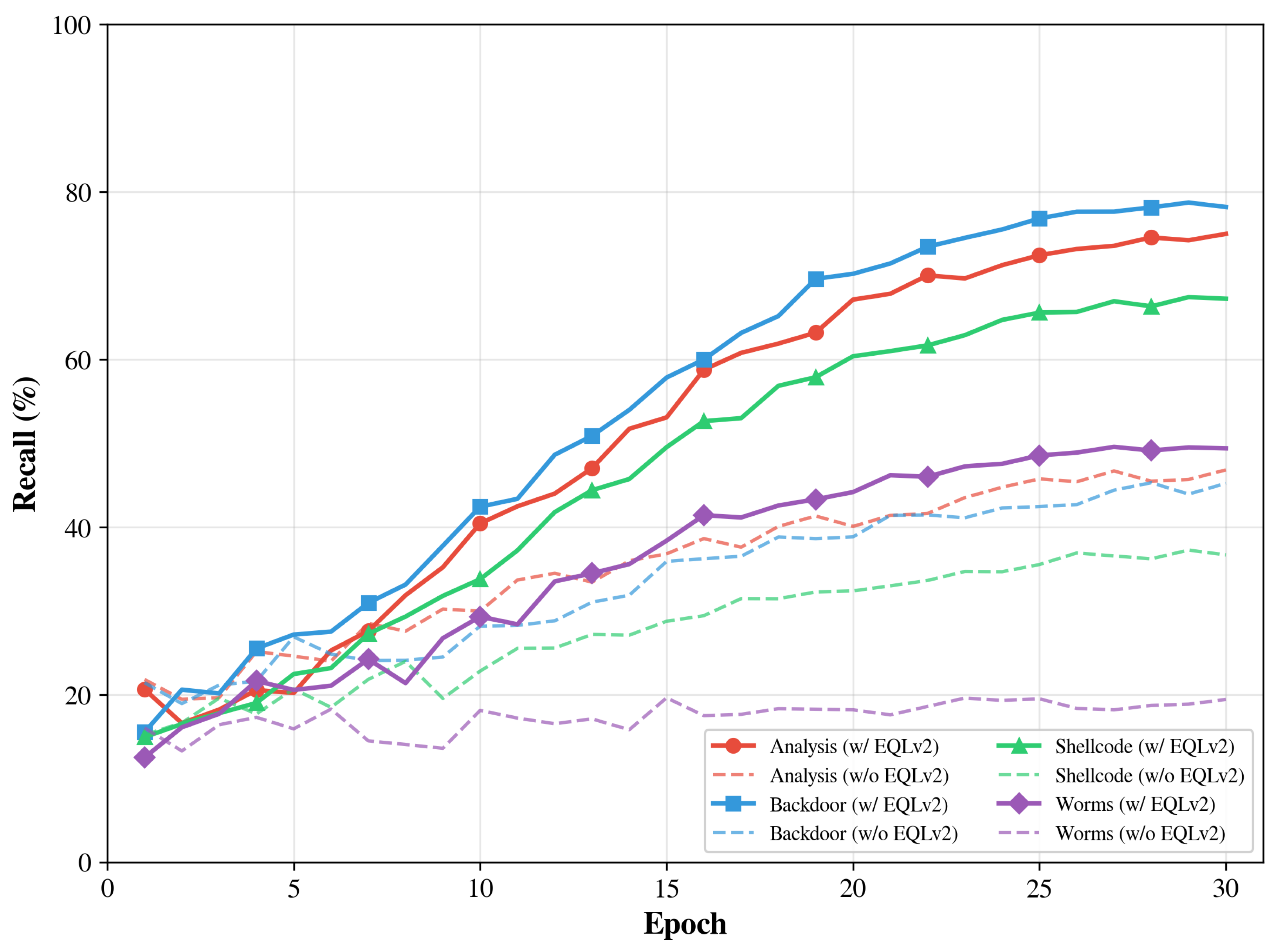
To further illustrate the actual regulatory effect of the EQLv2 gradient-balancing mechanism during training, we record the per-class recall curves throughout the training process on the UNSW-NB15 dataset, as shown in Figure 4. Since the core function of EQLv2 is to mitigate class imbalance and enhance the detection capability of minority classes, we select the four attack types with the fewest samples in this dataset for visualization analysis: Analysis, Backdoor, Shellcode, and Worms. These four attack types account for only 2.9% of the total training samples and represent the most severely imbalanced categories.

As observed from the figure, without EQLv2, the recall rates of all minority classes increase slowly and converge to relatively low values, with the Worms class reaching only approximately 20%, indicating that the model struggles to effectively learn the features of extremely rare classes under standard cross-entropy loss. After incorporating EQLv2, the recall rates of all minority classes improve significantly, with Analysis, Backdoor, Shellcode, and Worms achieving final recall rates of approximately 75%, 78%, 67%, and 49%, respectively, representing improvements of approximately 28, 35, 30, and 29 percentage points over the baseline. Furthermore, the recall curves with EQLv2 exhibit noticeably faster growth rates, demonstrating that the gradient-balancing mechanism accelerates the learning process for minority-class features. These results intuitively validate that EQLv2 effectively mitigates the negative impact of class imbalance on model training by dynamically adjusting the gradient contributions across different categories.

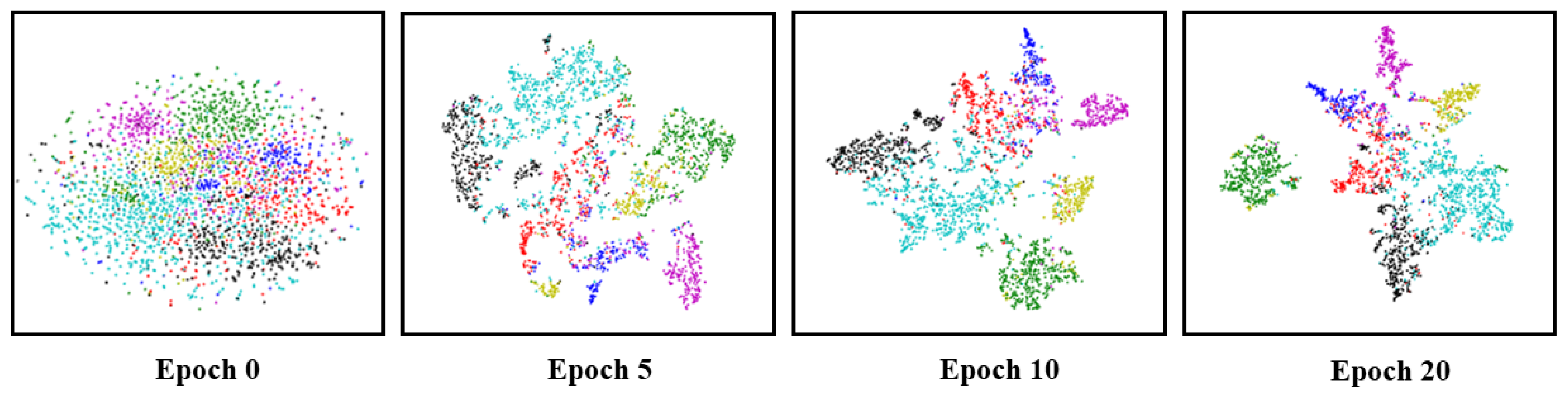
In addition, to visualize the feature learning process of GCNII, we apply t-SNE to project the learned feature representations at different training epochs, as shown in Figure 5. At epoch 0, features of all categories are randomly distributed and completely mixed. As training progresses, samples belonging to the same category gradually converge, forming well-separated clusters by epoch 20. This demonstrates that GCNII effectively learns discriminative features for distinguishing different traffic types.

5. Conclusions

Modern cyber attacks are characterized by pronounced multi-entity coordination and multi-stage evolution. Traditional intrusion detection methods, which inherently treat traffic records as independent samples, fail to effectively capture the resultant spatio-temporal coupling patterns. This fundamental limitation is exacerbated by severely degraded detection capability for rare attacks under conditions of extreme class imbalance. To address these critical challenges, this paper proposes the STEGCN, which reformulates the intrusion detection problem as a anomaly detection task on dynamic temporal graphs, thereby establishing a comprehensive technical pipeline from data representation to model optimization.

The core innovation of the STEGCN framework resides in the synergistic design of its constituent components. Specifically, a communication-relationship-driven graph construction strategy transforms discrete flow records into topology-aware structures. This is paired with GCNII, which extracts multi-scale spatial features, capturing both single-hop local anomalies and multi-hop global propagation patterns. Furthermore, the gating mechanisms of the GRU naturally align with the temporal dynamics of attack behaviors, enabling robust modeling of cross-stage attack chains. Finally, EQLv2 dynamically monitors per-class gradient ratios and adaptively adjusts weights to effectively break the dominance of majority classes over the optimization process.

Experimental validation demonstrated that STEGCN significantly outperforms state-of-the-art traditional machine learning methods and established deep learning approaches in both overall accuracy and recall, showing particularly pronounced effectiveness in addressing the challenges posed by class imbalance. By fundamentally shifting the detection paradigm from feature engineering on isolated flow records to the structured exploitation of network topology and temporal evolution, the proposed STEGCN model provides a systematic and robust solution for network intrusion detection. This framework holds substantial promise for enhancing real-world cybersecurity defense capabilities.

References

1. Anderson, J.P. Computer Security Threat Monitoring and Surveillance; Technical Report; James P. Anderson Company: Fort Washington, PA, USA, 1980. [Google Scholar]
2. Fang, L.; Li, Y.; Liu, Z.; Yin, C.; Li, M.; Cao, Z.J. A practical model based on anomaly detection for protecting medical IoT control services against external attacks. IEEE Trans. Ind. Inform. 2020, 17, 4260–4269. [Google Scholar] [CrossRef]
3. Zhang, H.; Zhang, X.; Zhang, Z.; Li, W. Summary of Intrusion Detection Models Based on Deep Learning. J. Comput. Eng. Appl. 2022, 58, 17–28. [Google Scholar]
4. Chao, C.; Jingkai, W.; Mei, C. An Intrusion Detection Algorithm for Wireless Sensor Networks Based on RBM-SVM. Comput. Appl. Softw. 2022, 39, 325–329. [Google Scholar]
5. Kanumalli, S.S.; Lavanya, K.; Rajeswari, A.; Samyuktha, P.; Tejaswi, M. A scalable network intrusion detection system using bi-lstm and cnn. In Proceedings of the 2023 Third International Conference on Artificial Intelligence and Smart Energy (ICAIS), Coimbatore, India, 2–4 February 2023; pp. 1–6. [Google Scholar]
6. Ullah, F.; Ullah, S.; Srivastava, G.; Lin, J.C.W. IDS-INT: Intrusion detection system using transformer-based transfer learning for imbalanced network traffic. Digit. Commun. Netw. 2024, 10, 190–204. [Google Scholar] [CrossRef]
7. Bilot, T.; El Madhoun, N.; Al Agha, K.; Zouaoui, A. Graph neural networks for intrusion detection: A survey. IEEE Access 2023, 11, 49114–49139. [Google Scholar] [CrossRef]
8. Sharafaldin, I.; Lashkari, A.H.; Ghorbani, A.A. Toward generating a new intrusion detection dataset and intrusion traffic characterization. ICISSp 2018, 1, 108–116. [Google Scholar]
9. Ren, K.; Yuan, S.; Zhang, C.; Shi, Y.; Huang, Z. CANET: A hierarchical cnn-attention model for network intrusion detection. Comput. Commun. 2023, 205, 170–181. [Google Scholar] [CrossRef]
10. Zhen, Z.; Yichen, Z.; Hongpeng, T. Network Intrusion Detection Based on Spatial Features and Generative Adversarial Networks. J. Zhengzhou Univ. Eng. Sci. 2024, 45, 40–47. [Google Scholar]
11. Hong, C.; Chaoyi, J.; Haibo, J.; Cong, W.; Jianbo, L. Fusion of Improved Stacked Encoder and Multi-Layer BiLSTM for Intrusion Detection Model. Comput. Eng. Appl. 2025, 61, 306–314. [Google Scholar]
12. Sha, Z.; Shengbing, C.; Youchen, K.; Xu, Z.; Shenyi, G. Network Intrusion Detection Based on Feature Selection and Spatio-Temporal Features. Comput. Eng. 2025, 51, 223–231. [Google Scholar]
13. Lo, W.W.; Layeghy, S.; Sarhan, M.; Gallagher, M.; Portmann, M. E-graphsage: A graph neural network based intrusion detection system for iot. arXiv 2021, arXiv:2103.16329. [Google Scholar]
14. Chang, L.; Branco, P. Graph-based solutions with residuals for intrusion detection: The modified e-graphsage and e-resgat algorithms. arXiv 2021, arXiv:2111.13597. [Google Scholar]
15. Xueli, S.; Shifeng, L. Intrusion Detection Model Based on Graph Edge Feature Attention. Comput. Eng. 2024, 50, 236–245. [Google Scholar]
16. Le, W.; Meng, H.; Xiaojuan, L.; Ni, Z.; Haodong, C. Review of Classification Methods for Unbalanced Data Sets. Comput. Eng. Appl. 2021, 57, 64606–64628. [Google Scholar]
17. Wei, W.; Chen, Y.; Lin, Q.; Ji, J.; Wong, K.C.; Li, J. Multi-objective evolving long–short term memory networks with attention for network intrusion detection. Appl. Soft Comput. 2023, 139, 110216. [Google Scholar] [CrossRef]
18. Yuan, L.; Yu, S.; Yang, Z.; Duan, M.; Li, K. A data balancing approach based on generative adversarial network. Future Gener. Comput. Syst. 2023, 141, 768–776. [Google Scholar] [CrossRef]
19. Liu, C.; Antypenko, R.; Sushko, I.; Zakharchenko, O. Intrusion detection system after data augmentation schemes based on the VAE and CVAE. IEEE Trans. Reliab. 2022, 71, 1000–1010. [Google Scholar] [CrossRef]
20. Tan, J.; Lu, X.; Zhang, G.; Yin, C.; Li, Q. Equalization loss v2: A new gradient balance approach for long-tailed object detection. In Proceedings of the IEEE/CVF Conference on Computer Vision and Pattern Recognition, Nashville, TN, USA, 20–25 June 2021; pp. 1685–1694. [Google Scholar]
21. Panigrahi, A.; Pati, A.; Addula, S.R.; Pati, A.K.; Sahoo, G.; Dash, M. An Ensemble Machine Learning-Based Model for Blockchain Transactional Data Classification. In Proceedings of the International Conference on Biologically Inspired Techniques in Many-Criteria Decision-Making Technologies; Springer: Cham, Switzerland, 2024; pp. 430–438. [Google Scholar]
22. Panigrahi, R.; Borah, S. A detailed analysis of CICIDS2017 dataset for designing Intrusion Detection Systems. Int. J. Eng. Technol. 2018, 7, 479–482. [Google Scholar]
23. Moustafa, N.; Slay, J. UNSW-NB15: A comprehensive data set for network intrusion detection systems (UNSW-NB15 network data set). In Proceedings of the 2015 Military Communications and Information Systems Conference (MilCIS), Canberra, ACT, Australia, 10–12 November 2015; pp. 1–6. [Google Scholar]
24. Chen, M.; Wei, Z.; Huang, Z.; Ding, B.; Li, Y. Simple and deep graph convolutional networks. In Proceedings of the International Conference on Machine Learning, PMLR, Virtual, 13–18 July 2020; pp. 1725–1735. [Google Scholar]
25. Upadhyay, A.; Thakur, N.; Pandey, A.; Khan, M.; Vibhute, A.D. Multiple Intrusion Detection in Complex Cloud Environments Using Random Forest and Deep Learning on the UNSW-NB15 Benchmark Datasets. In Proceedings of the International Conference on Intelligent Communication, Control and Devices; Springer: Singapore, 2024; pp. 71–85. [Google Scholar]
26. Mohamed, F.O.A.; Agarwal, M. Using recursive feature elimination feature selection based machine learning classifier for attack classification on UNSW-NB 15 dataset. In Proceedings of the 2024 IEEE 9th International Conference for Convergence in Technology (I2CT), Pune, India, 5–7 April 2024; pp. 1–7. [Google Scholar]
27. Sambandam, R.K.; Daniel, D.; Gokulapriya, R.; Vetriveeran, D.; Jenefa, J.; Anuneshwar. Comparison of Machine Learning-Based Intrusion Detection Systems Using UNSW-NB15 Dataset. In Proceedings of the International Conference on Artificial Intelligence on Textile and Apparel; Springer: Singapore, 2023; pp. 311–324. [Google Scholar]
28. Al-Obaidi, A.; Ibrahim, A.A.; Khaleel, A.M. The Effectiveness of Deploying Machine Learning Techniques in Information Security to Detect Nine Attacks: UNSW-NB15 Dataset as a Case Study. Math. Model. Eng. Probl. 2023, 10, 5. [Google Scholar] [CrossRef]
29. Hooshmand, M.K.; Hosahalli, D. Network anomaly detection using deep learning techniques. CAAI Trans. Intell. Technol. 2022, 7, 228–243. [Google Scholar] [CrossRef]
30. Kumar, A.; Soni, A.; Singh, M. Performing multiclass classification on UNSW-NB15 dataset by applying machine learning approach on intrusion detection system. In Proceedings of the International Conference on Data Science and Big Data Analysis; Springer: Singapore, 2023; pp. 461–473. [Google Scholar]
31. Jose, J.; Jose, D.V. Deep learning algorithms for intrusion detection systems in internet of things using CIC-IDS 2017 dataset. Int. J. Electr. Comput. Eng. (IJECE) 2023, 13, 1134–1141. [Google Scholar] [CrossRef]
32. Imrana, Y.; Xiang, Y.; Ali, L.; Abdul-Rauf, Z. A bidirectional LSTM deep learning approach for intrusion detection. Expert Syst. Appl. 2021, 185, 115524. [Google Scholar] [CrossRef]
33. Li, J.; Zhang, H.; Liu, Z.; Liu, Y. Network intrusion detection via tri-broad learning system based on spatial-temporal granularity. J. Supercomput. 2023, 79, 9180–9205. [Google Scholar] [CrossRef]
34. Zhang, H.; Li, J.L.; Liu, X.M.; Dong, C. Multi-dimensional feature fusion and stacking ensemble mechanism for network intrusion detection. Future Gener. Comput. Syst. 2021, 122, 130–143. [Google Scholar] [CrossRef]
35. Chen, Y.; Lin, Q.; Wei, W.; Ji, J.; Wong, K.C.; Coello, C. Intrusion detection using multi-objective evolutionary convolutional neural network for Internet of Things in Fog computing. Knowl.-Based Syst. 2022, 244, 108505. [Google Scholar] [CrossRef]
Figure 1. STEGCN model framework.
Electronics 15 00646 g001
Figure 2. The ROC curves of different models in the UNSW-NB15 dataset.
Electronics 15 00646 g002
Figure 3. The ROC curves of different models in the CICIDS2017 dataset.
Electronics 15 00646 g003
Figure 4. Effect of EQLv2 on minority-class recall during training on the UNSW-NB15 dataset.
Electronics 15 00646 g004
Figure 5. The visualization of learned features of the UNSW-NB15 dataset during training GCNII.
Electronics 15 00646 g005