Optimization of High-Frequency Transmission Line Reflection Wave Compensation and Impedance Matching Based on a DQN-GA Hybrid Algorithm

Abstract

In high-frequency circuit design, parameters such as the characteristic impedance and propagation constant of transmission lines directly affect key performance metrics, including signal integrity and power transmission efficiency. To address the challenge of optimizing impedance matching for high-frequency PCB transmission lines, this study applies a hybrid deep Q-network—genetic algorithm (DQN-GA) that integrates deep reinforcement learning with a genetic algorithm (GA). Unlike existing methods that primarily focus on predictive modeling or single-algorithm optimization, the proposed approach introduces a bidirectional interaction mechanism for algorithm fusion: transmission line structures learned by the deep Q-network (DQN) are encoded as chromosomes to enhance the diversity of the genetic algorithm population; simultaneously, high-fitness individuals from the genetic algorithm are decoded and stored in the experience replay pool of the DQN to accelerate its convergence. Simulation results demonstrate that the DQN-GA algorithm significantly outperforms both unoptimized structures and standalone GA methods, achieving substantial improvements in fitness scores and S11 transmission coefficients. This algorithm effectively overcomes the limitations of conventional approaches in addressing complex reflected wave compensation problems in high-frequency applications, providing a robust solution for signal integrity optimization in high-speed circuit design. This study not only advances the field of intelligent circuit optimization but also establishes a valuable framework for the application of hybrid algorithms to complex engineering challenges.

1. Introduction

In modern electronic systems, the printed circuit board (PCB) serves as a core component, undertaking critical tasks such as signal transmission, power distribution, and functional module integration. With the rapid advancement of fields like wireless communication, high-speed data transmission, and radar systems, the demand for high-frequency circuits has grown significantly, imposing stricter requirements on signal integrity and reliability. As the fundamental unit for signal transmission on PCBs, the design quality of transmission lines directly determines system performance and stability. However, in high-frequency applications, transmission lines face multiple challenges: skin effect and dielectric loss exacerbate signal attenuation, while impedance mismatch-induced reflected waves can lead to waveform distortion or even signal loss. Particularly when multiple capacitive load devices are connected to a bus, the non-uniformity of the transmission line further amplifies reflection interference. While traditional impedance matching methods, such as the Smith chart method and microstrip line design techniques, perform well in low-frequency ranges, they increasingly reveal limitations in high-frequency environments.

1.1. Related Works

To address the aforementioned issues, existing research has widely adopted optimization algorithms and machine learning methods. In the application of machine learning to high-speed channel modeling, Lu et al. [1] were the first to apply deep neural networks (DNNs) and support vector regression (SVR) to high-speed channel modeling, significantly reducing the computational cost of traditional simulations by predicting eye diagram metrics. However, this approach primarily focuses on performance prediction rather than optimization design and fails to fully exploit the synergistic effects between algorithms. The deep genetic algorithm (Deep GA) proposed by Zhang et al. [2] embeds DNNs into the genetic algorithm to accelerate the evaluation process, yet this method remains confined to a single optimization framework and does not effectively integrate the dynamic decision-making advantages of reinforcement learning. Lei et al. [3] developed a Generative Query Scheme (GQS) that enhances data efficiency through an active learning strategy, though its focus lies more on sample selection than on algorithmic fusion.

In recent years, the integration of reinforcement learning (RL) with metaheuristic algorithms has offered new avenues for tackling complex optimization problems. Regarding frameworks for algorithm fusion, the RLHO framework proposed by Cai et al. [4] pioneered the use of reinforcement learning to generate initial solutions for heuristic algorithms, achieving notable results in bin packing problems. Hong et al. [5] combined deep reinforcement learning with simulated annealing to address the traveling salesman problem, improving algorithm performance via a Transformer architecture and an action dropout layer. Seyyedabbasi et al. [6] systematically compared various hybrid strategies of RL and metaheuristic algorithms, confirming the superiority of such integrated approaches. Zou et al. [7] advanced the development of deep learning-based framework testing with their Ramos framework, which employs a hierarchical heuristic model for generation.

In the field of circuit design, reinforcement learning methods have also demonstrated significant potential. Choy et al. and Shoaee et al. [8,9] applied RL-based methods for decoupling capacitor placement in power integrity optimization, highlighting the promise of RL in circuit design. Zhou et al. [10] proposed a reinforcement active learning approach for signal integrity simulation. By modeling the data labeling problem as a Markov decision process, their method achieved a substantial reduction in required data volume within PCIe and DDR environments. Miao et al. [11] developed a deep reinforcement learning-based optimization method for CoWoS chip interconnect design. Utilizing a dueling double deep Q-network (DDQN), their approach balances signal integrity and interconnect density in signal/ground line layout. Kim et al. [12] introduced an automatic router based on the Transformer architecture and reinforcement learning, which simultaneously optimizes wire length, crosstalk, and via count in PCB routing.

Regarding hybrid methods combining genetic algorithms and RL, John et al. [13] proposed an approach integrating degenerate deep reinforcement learning with a genetic algorithm to compute the characteristic parameters of surface microstrip transmission lines. This physics-driven AI method achieved accurate predictions of impedance and effective dielectric constant. Song et al. [14] introduced a reinforcement learning genetic algorithm based on Q-learning, where Q-learning was embedded into an improved genetic algorithm to guide the population search process through intelligent decision-making. This approach delivered efficient optimization performance in the electromagnetic detection satellite scheduling problem. Yasunaga et al. [15] presented a design method for capacitive segmented transmission lines based on a genetic algorithm and cuckoo search. By utilizing reflected waves generated from impedance mismatch to compensate for signal distortion, their method achieved significant signal integrity improvement in the GHz frequency band. In the domain of PCB layout optimization, Vassallo et al. [16] introduced an adaptive reward-based reinforcement learning method, which formulates the PCB component layout problem as a Markov decision process. By employing the TD3 and SAC algorithms to learn basic layout techniques, their approach achieved a notable reduction in post-routing wire length compared to the simulated annealing method. Chen et al. [17] proposed a reinforcement learning method based on proximal policy optimization, where an agent predicts the optimal number of iterations for the simulated annealing algorithm. This strategy resulted in a more than 50% reduction in runtime for PCB layout tasks. Ooi et al. [18] developed a high-speed transmission line crosstalk modeling method using a multilayer perceptron neural network. Training data were generated through design of experiments, enabling accurate time-domain crosstalk prediction for both strip line and microstrip line configurations. In the broader context of hybrid algorithm research, Ma et al. [19] introduced a flexible job shop scheduling method based on a deep reinforcement learning-assisted adaptive genetic algorithm (DRL-A-GA). By representing the population state with a continuous state vector and designing four specialized mutation operations, their approach enables the adaptive adjustment of key parameters and evolutionary operators in the genetic algorithm. Radaideh and Shirvan [20] proposed a rule-based reinforcement learning method to guide evolutionary algorithms for constraint optimization. They employed proximal policy optimization to learn problem constraint rules and injected RL experience into algorithms such as genetic algorithms, simulated annealing, and particle swarm optimization, significantly enhancing exploration capability within constrained search spaces. Liu et al. [21] introduced the NeuroCrossover intelligent genetic locus selection algorithm, which employs a cross-information collaborative attention model and n-step proximal policy optimization to achieve intelligent selection of genetic loci for crossover operators in genetic algorithms. This approach has demonstrated significant improvements in solution quality and convergence speed when applied to the traveling salesman problem, the capacitated vehicle routing problem, and the bin packing problem.

1.2. Contributions

While existing methods have made progress in specific domains, the deep integration of genetic algorithms and reinforcement learning to address the reflected wave compensation problem in high-frequency transmission line design remains a research gap. Specifically, although GA is capable of global optimization, it is prone to local optima and exhibits slow convergence. RL possesses adaptive learning capabilities but suffers from low efficiency during the initial exploration phase. Current hybrid methods combining RL and metaheuristics predominantly focus on improving a single algorithm, failing to fully leverage the synergistic effects of bidirectional interaction.

The main contributions of this paper include the following:

A Bidirectional Interaction Algorithm Fusion Mechanism: Unlike traditional unidirectional transmission line enhancement strategies, the adapted DQN-GA framework achieves deep bidirectional interaction between reinforcement learning and the genetic algorithm. By encoding the structural schemes learned by DQN into chromosomes and injecting them into the GA population, population diversity is enhanced; meanwhile, high-fitness individuals from the GA are decoded and added to the DQN experience pool, accelerating model convergence and exploration efficiency.

Engineering practicality: The algorithm incorporates manufacturing-aware parameters (such as microstrip line characteristics), providing a foundation for practical implementation. While current manufacturing tolerances limit physical verification, the simulation framework establishes a methodology that can be validated under higher-precision conditions, offering a pathway toward real-world impedance matching applications.

Comparative advantages over existing methods: Compared to the pure prediction model of Lu et al. [1], DQN-GA achieves a leap from prediction to optimization, directly optimizing design parameters; compared to the Deep GA of Zhang et al. [2], this method addresses GA’s tendency to fall into local optima and RL’s low initial efficiency through bidirectional interaction between reinforcement learning and genetic algorithms; compared to the RLHO of Cai et al. [4] and the RL-SA of Hong et al. [5], DQN-GA focuses more on deep integration at the algorithmic level, rather than merely data sampling or parameter adjustment strategies. In the field of circuit design, compared to the power integrity optimization methods proposed by Choy [8] and Shoaee [9], the present method specifically addresses impedance matching issues in high-frequency transmission lines, offering a more specialized solution.

Simulation results demonstrate that DQN-GA achieves superior S-parameter performance and routing design in impedance matching scheme design, showing significant improvements across multiple metrics compared to pure DQN or pure GA approaches. This research not only provides a new technical pathway for high-frequency circuit design but also offers a referable algorithm fusion framework for optimization problems in complex environments.

2. Materials and Methods

2.1. Problem Modeling and Circuit Structure

To systematically address issues mentioned in Section 1, this study employs a segmented transmission line (STL) design approach. Its core concept is to utilize the reflected waves generated by impedance mismatches between adjacent segments as compensation signals. By designing and adjusting the length and impedance characteristics of each transmission line segment, these reflected waves can be superimposed onto the distorted transmission signal, thereby achieving effective compensation of the signal waveform [15]. This approach not only adapts to the complex conditions of high-frequency environments but also significantly enhances transmission performance in the presence of multiple capacitive loads.

2.1.1. Circuit Model and Optimization Problem Definition

Figure 1 illustrates the optimization target of this study: a ten-segment transmission line circuit with distributed capacitive loads. This circuit models a typical scenario in practical high-frequency PCB design, where multiple capacitive load devices are powered. The circuit structure is as follows:

where

• V: AC excitation source (1 V, frequency sweep from 200 to 800 MHz);
• R₁: Series input resistor (optimization variable);
• R_t: Parallel termination resistor (optimization variable);
• C₁ = 10 pF: Capacitive load located between the fourth and fifth transmission line segments;
• C₂ = 20 pF: Capacitive load located between the eighth and ninth transmission line segments;
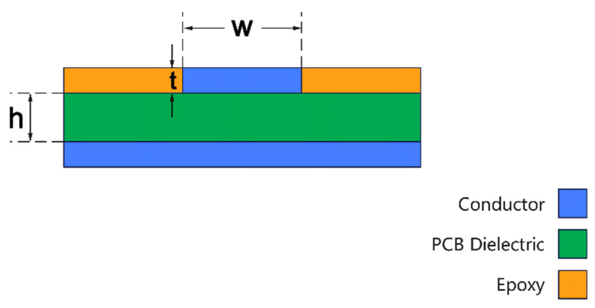
• T₁–T₁₀: Ten transmission line segments, each with its characteristic impedance Z_0,i and time delay Td (corresponding to physical length l_i) as optimization variables.

The circuit was analyzed in the frequency domain for S-parameters using LTspice. The simulation settings, as shown below the schematic, are as follows: .ac oct 100 200 Meg 800 Meg. This indicates an AC sweep from 200 MHz to 800 MHz with a density of 100 points per octave. The optimization achieves the desired impedance profile by adjusting the trace width along a straight microstrip line, which represents a planar layout optimization approach.

Table 1. Circuit component parameters.

Component	Symbol	Parameter	Value/Range	Status
V	Excitation	Type/Amplitude/Freq.	AC 1 V, 200–800 MHz	Fixed
R1	Input Resistor	Resistance	10–910 Ω (E24)	Variable
Rt	Termination Resistor	Resistance	10–910 Ω (E24)	Variable
C1	Capacitive Load 1	Capacitance	10 pF (T4-T5)	Fixed
C2	Capacitive Load 2	Capacitance	20 pF (T8-T9)	Fixed
T1–T10	Transmission Lines	Z0,i	{47.4, 42.7, 37.2, 30.7, 26.2} Ω	Variable
		Unit Delay Tdi	{146.8, 147.9, 149.3, 151.2, 152.8} ps/inch	Variable
		Length li	0.1–2.0 inches	Variable
Constraint	Total Length	Σli	5.0 inches	Hard

Note: Z_0,i values correspond to microstrip widths based on FR4 (ε_r = 3.9, t = 5 mil). Under the lossless approximation, it is a real number.

details the parameter settings for all components in Figure 1. The optimization variables include the transmission line parameters, specifically the characteristic impedance Z_0,i and length l_i for each segment, as well as the resistor values R₁ and R_t. The fixed parameters are the capacitive loads C₁ = 10 pF and C₂ = 20 pF. The characteristic impedance Z_0,i for each transmission line segment is selected from five predefined values, corresponding to different microstrip line widths. The length l_i of each segment satisfies the total length constraint Σl_i = 5.0 inches.

2.1.2. Physical Implementation and Modeling Assumptions

Figure 2 illustrates the physical structure used to implement each transmission line segment T_i: a surface microstrip line. In microstrip line or stripline structures, the characteristic impedance Z_0,i is a function of the transmission line width W_i, expressed as follows:

$$Z_{0,i}={\displaystyle \frac{87}{\sqrt{{\epsilon }_r+1.41}}}\ln {\displaystyle \frac{5.98h}{0.8W_i+t}}$$

(1)

where h = 5 mil is the dielectric thickness, ε_r = 3.9 is the relative permittivity of the FR4 dielectric, and T = 1.4 mil is the copper thickness. Consequently, adjusting Z_0,i is equivalent to adjusting W_i. In the engineering design process, the impedance Z_0,i is controlled via the W_i value of the transmission line.

The electromagnetic simulation model employs standard FR4 high-frequency PCB material parameters. Copper trace conductivity is σ = 5.8 × 10⁷ S/m, corresponding to 1 oz copper foil (35 μm thickness). The FR4 substrate exhibits a relative permittivity of ε_r = 3.9 with a loss tangent of tanδ = 0.02 at the operating frequency range. The relative permeability is μ_r = 1 for non-magnetic dielectric materials.

Modeling Assumptions and Scope Definition:

This study confines the optimization scope to the vertical structural parameters of the transmission line, specifically line width and dielectric properties, as these are the dominant factors influencing characteristic impedance and reflected wave compensation. Under the constraint of a fixed total length, planar layout features such as bends and corners are treated as secondary factors and are proposed as subjects for future research. Regarding the simulation methodology, a frequency-domain harmonic steady-state analysis is employed using a frequency-domain port as the excitation source, which is well suited for S-parameter evaluation. The transmission line is modeled using the lossless T-element in LTspice, characterized by its characteristic impedance Z_0,i and time delay Td_i. Finally, the material parameters are fixed to standard values: FR4 dielectric (ε_r = 3.9, tanδ = 0.02) and copper conductors (σ = 5.8 × 10⁷ S/m).

2.1.3. Reflected Wave Compensation Mechanism

The core innovation of this method lies in utilizing reflected waves generated by intelligently designed impedance discontinuities as compensation signals. As shown in Figure 1, capacitive loads C₁ and C₂ introduce a significant impedance mismatch, generating reflected waves that cause signal distortion. By optimizing the characteristic impedance Z_0i and length l_i of each transmission line segment, the following can be controlled:

• The amplitude of the reflected wave, which is determined by the impedance ratio Z_0,(i+1)/Z_0,i of adjacent segments.
• The phase of the reflected wave, which is determined by the propagation delay 2 × ΣTd_i.

The optimization objective is to ensure that the reflected wave generated from a preceding segment, after an appropriate delay, superimposes in-phase with the main signal at the capacitive load location, thereby compensating for the signal attenuation caused by the capacitive load. This “using reflection to counteract reflection” approach is particularly suitable for high-frequency transmission line design with distributed capacitive loads. By superimposing the reflected waves generated at the interfaces between adjacent characteristic impedances Z_0,i and Z_0,(i+1), and by adjusting the characteristic impedance Z_0,i, length l_i, input resistor R₁, and termination resistor R_t of each transmission line segment, an ideal signal waveform can be obtained at the destination.

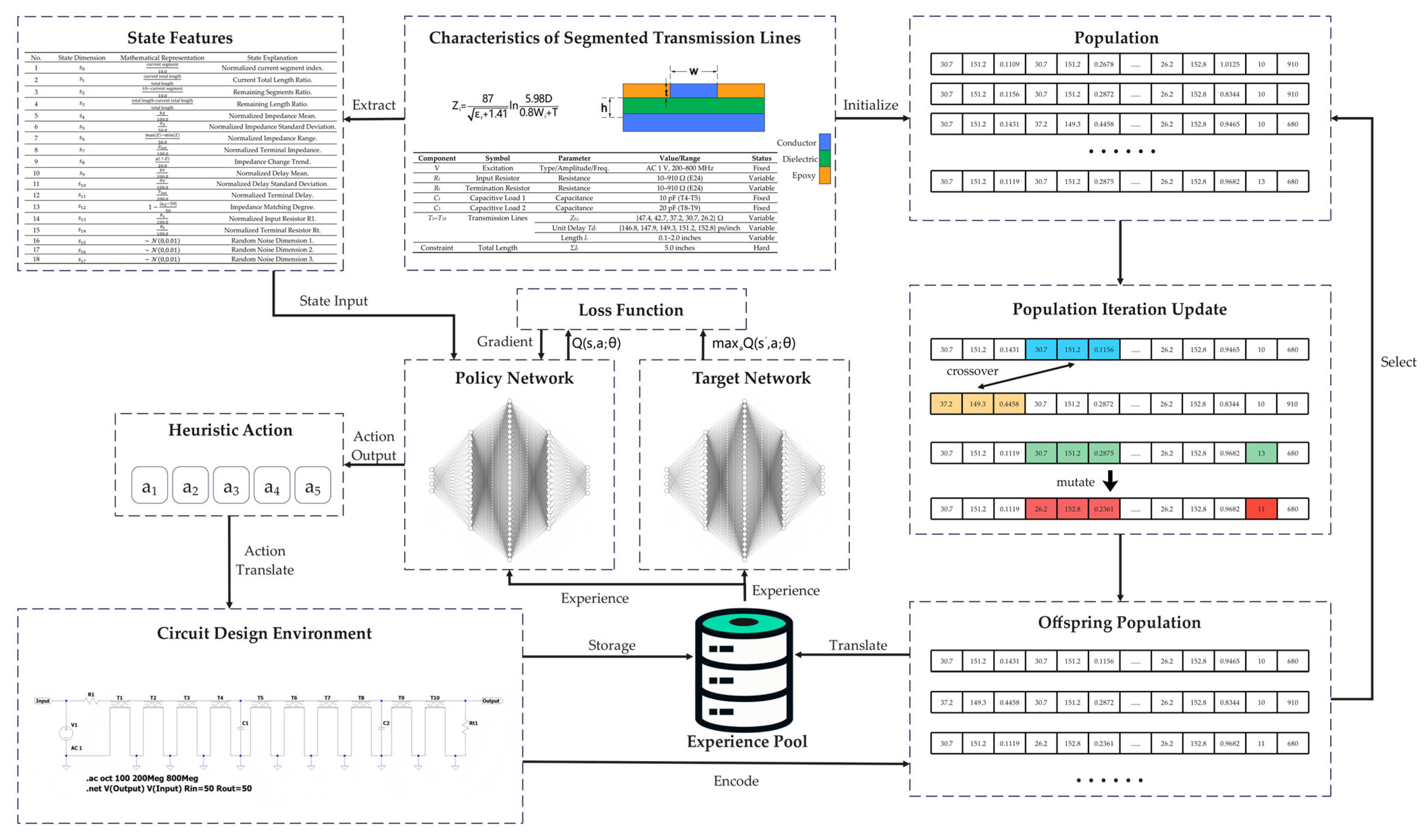
2.2. The DQN-GA Algorithm: Integrating Deep Q-Learning with Genetic Algorithm

The DQN-GA algorithm is a dynamic programming approach proposed by Xu et al. [22] that integrates a deep reinforcement learning algorithm with a genetic algorithm. Our DQN-GA integration introduces two key innovations: reformulating impedance matching as a Markov decision process with specialized state representation for transmission line parameters and establishing a bidirectional knowledge transfer mechanism where DQN-learned policies guide GA evolution while GA-discovered elites enrich DQN’s experience pool. Initially, the agent in the DQN interacts with the environment and, through multiple training episodes, learns a relatively optimal segmented transmission line structure. In this process, the electrical parameters of microstrip lines corresponding to various trace widths under actual fabrication constraints are provided as the action selection space. Subsequently, this structure is encoded by treating the characteristic impedance Z₀ and propagation delay Td of each transmission line segment as a gene. These genes are then sequentially arranged to form a fixed-length chromosome, which is introduced into the population of the genetic algorithm. The chromosomes generated by the DQN method supply initial solutions to the genetic algorithm, thereby accelerating its search process. Subsequently, the individuals with high fitness values in the genetic algorithm are decoded, and the decoded assembly sequences are added to the experience pool of DQN. By incorporating the decoded high-fitness individuals from the genetic algorithm into the experience pool, more segmented transmission line structures with maximum S₂₁ parameters and minimum S₁₁ parameters are obtained as training data, guiding the agent to learn effective design strategies.

The method achieves synergistic optimization between the algorithms through a bidirectional interaction mechanism: on one hand, the DQN agent learns transmission line structure design strategies by interacting with the simulation environment and encodes the generated solutions as chromosomes to inject into the GA population, thereby enhancing population diversity; on the other hand, high-fitness individuals from GA are decoded into state-action sequences and added to DQN’s experience replay pool, accelerating DQN’s convergence and exploration efficiency. This bidirectional interaction not only addresses the issues of traditional genetic algorithms being prone to local optima and the low initial exploration efficiency of DQN but also enhances the algorithm’s adaptability in dynamic design environments. The reward function in the DQN component and the fitness function in the GA component share the same core functional structure to ensure consistency in the optimization direction. Figure 3 illustrates the overall architecture of the DQN-GA framework, including the DQN module, the GA module, and the bidirectional interaction process.

Figure 3 illustrates the proposed hybrid optimization framework integrating the deep Q-network and genetic algorithm. The architecture consists of three core components:

• DQN Component (left side):
  • State Network: Receives the transmission line parameter state vector s_t.
  • Experience Replay Pool: Stores historical experiences (s_t, a_t, r_t+1, s_t+1).
  • Q-value Update: Updates network parameters via temporal-difference learning.
  • Storage: Store the optimal solution in the experience pool.
• GA Component (right side):
  • Population Initialization: Generates an initial set of chromosomes.
  • Genetic Operations: Selection, crossover, and mutation.
  • Fitness Evaluation: Computes the fitness value for each individual.
  • Translate and storage: Select optimal offspring and store them in the experience pool.
• Bidirectional interaction mechanism (center):
  • DQN → GA direction: The policy parameters learned by the DQN are encoded into GA chromosomes to guide population evolution.
  • GA → DQN direction: The elite individuals discovered by the GA search are decoded into training experiences for the DQN, thereby enriching the experience pool.

This synergistic mechanism enables the algorithm to effectively combine local policy optimization with global space search.

2.2.1. DQN Component Design

The DQN approach employs a deep neural network to approximate the optimal action-value function $Q*(\mathit{s},a)$ by predicting $Q(\mathit{s},a;\mathit{\theta })$, where θ represents the parameters of the neural network. Training is conducted using experience replay. In reinforcement learning, the action-value function is updated according to Equation (2). In DQN, the network $Q(\mathit{s},a;\mathit{\theta })$ replaces the conventional $Q(\mathit{s},a)$ in reinforcement learning; consequently, updating $Q(\mathit{s},a;\mathit{\theta })$ is essentially equivalent to updating the parameters θ. The action-value function $Q(\mathit{s},a;\mathit{\theta })$ in the DQN is given by Equation (3).

$$Q(\mathit{s},a)\leftarrow Q(\mathit{s},a)+\alpha \left[r(\mathit{s},a,{\mathit{s}}^{\prime })+\gamma \underset{a^{\prime }}{\mathrm{m}\mathrm{a}\mathrm{x}}Q\left({\mathit{s}}^{\prime },a^{\prime }\right)-Q(\mathit{s},a)\right]$$

(2)

$$Q(\mathit{s},a;\mathit{\theta })\approx r+\gamma \underset{a}{\mathrm{m}\mathrm{a}\mathrm{x}}Q({\mathit{s}}^{\prime },a;\mathit{\theta })$$

(3)

Here, s denotes the current state, s’ represents the next state after executing action a, γ is the discount factor, α is the learning rate, and θ denotes the parameters (weights) of the neural network. $Q(\mathit{s},a)$ is the action-value function (Q-value), which estimates the long-term expected return for selecting action a in state s. $r(\mathit{s},a,{\mathit{s}}^{\prime })$ is the immediate reward, representing the one-step reward obtained when transitioning from state s to state s’ after taking action a. $Q(\mathit{s},a;\mathit{\theta })$ is the parameterized action-value function (Q-function), which approximates the long-term expected return for choosing action a in state s through the parameters θ.

The parameters θ of the neural network are updated via gradient descent and backpropagation. At each time step, the network selects an action based on the current state and computes the corresponding reward. Subsequently, the gradient is calculated using a loss function based on the error between the actual reward and the predicted value, and the parameters are updated through gradient descent. In the DQN, there are two neural networks with identical architectures but different parameters: the target network $Q(\mathit{s},a;\mathit{\theta })$ and the prediction network $Q*(\mathit{s},a)$. The network parameters are updated periodically. The parameter update expression is given by Equation (4).

$${\mathit{\theta }}_{t+1}={\mathit{\theta }}_{\mathit{t}}+\alpha \left[r+\gamma \underset{a^{\prime }}{\max }Q\left({\mathit{s}}^{\prime },a^{\prime };{\mathit{\theta }}^{-}\right)-Q\left(\mathit{s},a;\mathit{\theta }\right)\right]\nabla Q\left(\mathit{s},a;\mathit{\theta }\right)$$

(4)

Here, θ_t represents the parameters of the current neural network, and θ_t+1 denotes the updated parameters. θ⁻ refers to the parameters of the target network, which is a separate, independent neural network used for calculating the target Q-value. The DQN component of the DQN-GA algorithm approximates the Q-value function using a neural network to guide design decisions for the transmission line structure. Its core components include the state space, action space, reward function, and the neural network architecture.

State Design: In the DQN-GA algorithm, state design constitutes a core component for the reinforcement learning agent to perceive its environment. Its objective is to encode the dynamic construction process of a segmented transmission line circuit into a low-dimensional, information-rich vector representation. The state vector must comprehensively capture the parameters of the transmission line segments, the resistor configuration, and the statistical characteristics of historical sequences to guide the agent in making efficient decisions within the action space. The DQN component employs an 18-dimensional state vector to represent the transmission line structure described in Section 2.1. Its composition is detailed as follows (as shown in

Table 2. State characteristics of segmented transmission lines.

No.	State Dimension	Mathematical Representation	State Explanation
1	$s_0$	${\displaystyle \frac{\mathrm{current} \mathrm{segment}}{10.0}}$	Normalized current segment index.
2	$s_1$	${\displaystyle \frac{\mathrm{current} \mathrm{total} \mathrm{length}}{\mathrm{total} \mathrm{length}}}$	Current Total Length Ratio.
3	$s_2$	${\displaystyle \frac{10-\mathrm{current} \mathrm{segment}}{10.0}}$	Remaining Segments Ratio.
4	$s_3$	${\displaystyle \frac{\mathrm{total} \mathrm{length}-\mathrm{current} \mathrm{total} \mathrm{length}}{\mathrm{total} \mathrm{length}}}$	Remaining Length Ratio.
5	$s_4$	${\displaystyle \frac{{\mathsf{\mu }}_Z}{100.0}}$	Normalized Impedance Mean.
6	$s_5$	${\displaystyle \frac{{\mathsf{\sigma }}_z}{50.0}}$	Normalized Impedance Standard Deviation.
7	$s_6$	${\displaystyle \frac{\max \left(Z\right)-\min \left(Z\right)}{50.0}}$	Normalized Impedance Range.
8	$s_7$	${\displaystyle \frac{Z_{\mathrm{last}}}{100.0}}$	Normalized Terminal Impedance.
9	$s_8$	${\displaystyle \frac{\mathsf{\mu }\left(\mathsf{\Delta }Z\right)}{20.0}}$	Impedance Change Trend.
10	$s_9$	${\displaystyle \frac{{\mathsf{\mu }}_T}{200.0}}$	Normalized Delay Mean.
11	$s_{10}$	${\displaystyle \frac{{\mathsf{\sigma }}_T}{100.0}}$	Normalized Delay Standard Deviation.
12	$s_{11}$	${\displaystyle \frac{T_{\mathrm{last}}}{200.0}}$	Normalized Terminal Delay.
13	$s_{12}$	$1-{\displaystyle \frac{\left|{\mathsf{\mu }}_Z-50\right|}{50}}$	Impedance Matching Degree.
14	$s_{13}$	${\displaystyle \frac{R_1}{100.0}}$	Normalized Input Resistor R1.
15	$s_{14}$	${\displaystyle \frac{R_{\mathrm{t}}}{100.0}}$	Normalized Terminal Resistor Rt.
16	$s_{15}$	$\sim \mathcal{N}\left(\mathrm{0,0.01}\right)$	Random Noise Dimension 1.
17	$s_{16}$	$\sim \mathcal{N}\left(\mathrm{0,0.01}\right)$	Random Noise Dimension 2.
18	$s_{17}$	$\sim \mathcal{N}\left(\mathrm{0,0.01}\right)$	Random Noise Dimension 3.

):

1.

Segment progress information (dimensions 0–3):

• Current segment index normalization ($s_0$): Reflects the progress of transmission line construction.
• Current total length normalization ($s_1$): Represents the proportion of constructed length to the total length (5.0 inches).
• Remaining segment count normalization ($s_2$): Quantifies the number of segments yet to be completed.
• Remaining length normalization ($s_3$): Indicates the remaining construction space.

Significance: These dimensions provide the agent with spatiotemporal context for the construction process, preventing invalid actions such as allocating excessive length.

2.

Impedance statistical features (dimensions 4–8):

• Impedance mean normalization ($s_4$): Captures the average level of historical impedance.
• Impedance standard deviation normalization ($s_5$): Measures the degree of impedance fluctuation.
• Impedance range normalized ($s_6$): Reflects the range of impedance variation.
• Terminal impedance normalized ($s_7$): Emphasizes the impedance value of the most recent segment.
• Impedance change trend ($s_8$): Calculates the mean of impedance differences between adjacent segments, characterizing the sequence dynamics.

Significance: These statistical measures compress the high-dimensional impedance sequence, highlighting overall matching quality and local variations, thereby replacing the raw sequence to reduce the state dimensionality.

3.

Delay statistical features (dimensions 9–11):

• Delay mean normalized ($s_9$).
• Delay standard deviation normalized ($s_{10}$).
• Terminal delay normalized ($s_{11}$).

Significance: Delay parameters affect the signal propagation phase. Their statistical features assist the agent in coordinating the coupling relationship between impedance and delay.

4.

Impedance Matching Degree (dimension 12):

• Target Matching Degree ($s_{12}$): Quantifies the deviation of the current average impedance from the target value (50 Ω). A value closer to 1 indicates better matching.

Significance: Directly relates to the reflected wave compensation objective, providing an intermediate signal for the reward function.

5.

Resistance Information (dimensions 13–14):

• Normalized Input Resistance R1 ($s_{13}$).
• Normalized Termination Resistance Rt ($s_{14}$).

Significance: Incorporates key circuit resistance parameters into the state, ensuring the agent simultaneously considers resistance configuration while optimizing transmission line segmentation, thereby enhancing overall impedance matching performance.

6.

Exploration–Enhancing Noise (dimensions 15–17):

Significance: Random Gaussian Noise ($s_{15}$~$s_{17}$): Injects a small amount of noise to improve the robustness of policy exploration and prevent premature convergence to a local optimum.

Action Design: In the DQN component of the DQN-GA algorithm, the design of actions directly determines the decision-making capability of the agent during the transmission line structure design process. Considering the discrete nature of transmission line parameters and manufacturing constraints in practical engineering applications, this study employs an action space design based on predefined transmission line characteristics, rather than a continuous parameter space. This approach not only aligns with the requirements of actual PCB manufacturing processes but also significantly reduces the exploration complexity of the algorithm.

Definition of the action space: The action space is composed of a predefined set of transmission line characteristics, where each action corresponds to a specific impedance-delay characteristic pair. Based on the code implementation, the action space can be expressed as follows:

$$\mathcal{A}=\left\{a_k\right|a_k=(Z_0^{\left(k\right)},T{d}^{\left(k\right)}),k=\mathrm{1,2},\dots ,\mathrm{K}\}$$

(5)

Here, $\mathrm{K}$ denotes the number of predefined characteristics, while $z_0^{\left(k\right)}$ and $T{d}^{\left(k\right)}$ represent the characteristic impedance (unit: Ω) and the unit delay (unit: ps/inch) corresponding to the $k$-th characteristic, respectively. In this study, $\mathrm{K}=5$, and the specific characteristic values are listed in

Table 3. Characteristic parameters of segmented transmission lines.

Action Index	Characteristic Impedance Z0 (Ω)	Unit Delay Td (ps/inch)
0	47.4	146.8
1	42.7	147.9
2	37.2	149.3
3	30.7	151.2
4	26.2	152.8

Note: The characteristic impedance values are magnitudes based on lossless transmission line model.

.

Note: The characteristic impedance values are magnitudes based on lossless transmission line model.

Action Implementation Mechanism: At each decision step t, the agent selects an action $a_t\in \mathcal{A}$ based on the current state s_t. The specific implementation process is as follows:

• Feature Selection: The agent selects an action index $k_t$ from a predefined feature set, employing either an ε-greedy strategy or neural network Q-value prediction.

• Length Determination: Once a feature is selected, the length $L_t$ of the transmission line segment is determined via an adaptive mechanism:

$$L_t=\left\{\begin{array}{c}{L}_{\mathrm{r}\mathrm{e}\mathrm{m}\mathrm{a}\mathrm{i}\mathrm{n}\mathrm{i}\mathrm{n}\mathrm{g}}\mathrm{if} n_{\mathrm{r}\mathrm{e}\mathrm{m}\mathrm{a}\mathrm{i}\mathrm{n}\mathrm{i}\mathrm{n}\mathrm{g}}=1\\ \max \left(0.1,\overline{L}+\mathsf{\Delta }L\right)\mathrm{otherwise}\end{array}\right.$$

(6)

Here, $L_{\mathrm{r}\mathrm{e}\mathrm{m}\mathrm{a}\mathrm{i}\mathrm{n}\mathrm{i}\mathrm{n}\mathrm{g}}$ denotes the total remaining length, ${ n}_{\mathrm{r}\mathrm{e}\mathrm{m}\mathrm{a}\mathrm{i}\mathrm{n}\mathrm{i}\mathrm{n}\mathrm{g}}$ is the number of remaining segments, $\overline{L}=L_{\mathrm{r}\mathrm{e}\mathrm{m}\mathrm{a}\mathrm{i}\mathrm{n}\mathrm{i}\mathrm{n}\mathrm{g}}/n_{\mathrm{r}\mathrm{e}\mathrm{m}\mathrm{a}\mathrm{i}\mathrm{n}\mathrm{i}\mathrm{n}\mathrm{g}}$ represents the average length, and $\mathsf{\Delta }L\sim \mathcal{N}\left(\mathrm{0,0.2}\overline{L}\right)$ is a length perturbation.

• Parameter Update: The selected features $(Z_0^{\left(k\right)},T{d}^{\left(k\right)})$ and the computed length $L_t$ are added to the current transmission line structure, updating the environment state.

Action Constraint Handling: To ensure the generated transmission line structure complies with physical constraints, the following constraint mechanisms are implemented during action execution:

• Total Length Constraint: The sum of all segment lengths is strictly equal to the total length of 5.0 inches, enforced via a dynamic adjustment mechanism. The scaling factor is calculated as follows:

$$\mathrm{s}\mathrm{c}\mathrm{a}\mathrm{l}\mathrm{e}\mathrm{f}\mathrm{a}\mathrm{c}\mathrm{t}\mathrm{o}\mathrm{r}={\displaystyle \frac{\mathrm{t}\mathrm{o}\mathrm{t}\mathrm{a}\mathrm{l} \mathrm{l}\mathrm{e}\mathrm{n}\mathrm{g}\mathrm{t}\mathrm{h}}{\mathrm{c}\mathrm{u}\mathrm{r}\mathrm{r}\mathrm{e}\mathrm{n}\mathrm{t} \mathrm{t}\mathrm{o}\mathrm{t}\mathrm{a}\mathrm{l} \mathrm{l}\mathrm{e}\mathrm{n}\mathrm{g}\mathrm{t}\mathrm{h}}}$$

(7)

$$\mathrm{a}\mathrm{d}\mathrm{j}\mathrm{u}\mathrm{s}\mathrm{t}\mathrm{e}\mathrm{d} \mathrm{l}\mathrm{e}\mathrm{n}\mathrm{g}\mathrm{t}\mathrm{h}=\mathrm{l}\mathrm{e}\mathrm{n}\mathrm{g}\mathrm{t}\mathrm{h} \mathrm{s}\mathrm{c}\mathrm{a}\mathrm{l}\mathrm{e} \mathrm{f}\mathrm{a}\mathrm{c}\mathrm{t}\mathrm{o}\mathrm{r}$$

(8)

• Fabrication Feasibility Constraint: All impedance values are drawn from a predefined set achievable with practical microstrip line fabrication processes, preventing unrealistic design proposals.
• Sequence Integrity Constraint: When the current segment index reaches 10, the action selection process is terminated, completing the construction of the transmission line structure.

Design of the Reward Function: The reward function serves as the core guiding signal for the DQN algorithm, directly determining the agent’s learning direction and optimization objectives. Considering the specific characteristics of the PCB transmission line impedance matching problem, this study designs a multi-objective reward function to simultaneously optimize signal transmission efficiency and reflection loss.

Composition of the Reward Function: The reward function $r_t$ consists of a base reward and an auxiliary reward, with the specific form as follows:

$$r_t=r_{\mathrm{b}\mathrm{a}\mathrm{s}\mathrm{e}}+r_{\mathrm{a}\mathrm{u}\mathrm{x}\mathrm{i}\mathrm{l}\mathrm{i}\mathrm{a}\mathrm{r}\mathrm{y}}$$

(9)

The base reward is based on the final S-parameter performance and adopts a weighted combination form:

$$r_{\mathrm{b}\mathrm{a}\mathrm{s}\mathrm{e}}=S_{\mathrm{21,500}\mathrm{M}\mathrm{H}\mathrm{z}}+0.02\cdot \left|S_{\mathrm{11,500}\mathrm{M}\mathrm{H}\mathrm{z}}\right|$$

(10)

Here, S_{21,500 MHz} denotes the transmission coefficient (unit: dB) at the 500 MHz frequency point, where a larger value indicates higher signal transmission efficiency; S_{11,500 MHz} denotes the reflection coefficient (unit: dB) at the 500 MHz frequency point, where a smaller absolute value indicates lower reflection loss. The weighting coefficient 0.02 balances the relative importance of these two optimization objectives and is an empirical coefficient derived from engineering practice.

The auxiliary rewards comprise several items related to engineering constraints:

• Length matching reward:

$$r_{\mathrm{l}\mathrm{e}\mathrm{n}\mathrm{g}\mathrm{t}\mathrm{h}}=\left\{\begin{array}{c}0.5\mathrm{if}\left|L_{\mathrm{t}\mathrm{o}\mathrm{t}\mathrm{a}\mathrm{l}}-5.0\right|<0.01\\ 0\mathrm{otherwise}\end{array}\right.$$

(11)

An additional reward is granted when the total length error is less than 0.01 inches, ensuring the design complies with physical constraints.

• Impedance matching reward (intermediate step):

$$r_{\mathrm{i}\mathrm{m}\mathrm{p}\mathrm{e}\mathrm{d}\mathrm{a}\mathrm{n}\mathrm{c}\mathrm{e}}=\left(1-{\displaystyle \frac{|\overline{Z}-50|}{50}}\right)\cdot 0.1$$

(12)

where $\overline{Z}$ is the current average impedance. This reward encourages the agent to maintain an impedance close to the target value of 50 Ω during the construction process.

The complete reward function is expressed as follows:

$$r_t=S_{\mathrm{21,500}\mathrm{M}\mathrm{H}\mathrm{z}}+0.02\cdot \left|S_{\mathrm{11,500}\mathrm{M}\mathrm{H}\mathrm{z}}\right|+r_{\mathrm{l}\mathrm{e}\mathrm{n}\mathrm{g}\mathrm{t}\mathrm{h}}+r_{\mathrm{i}\mathrm{m}\mathrm{p}\mathrm{e}\mathrm{d}\mathrm{a}\mathrm{n}\mathrm{c}\mathrm{e}}$$

(13)

• Multi-Objective Optimization Strategy: The design of the reward function embodies a balance among the following optimization objectives:
• Maximizing transmission efficiency: The term S_{21,500 MHz} encourages a high transmission coefficient, directly corresponding to a core metric of signal integrity.
• Minimizing reflection loss: The term |S_{11,500 MHz}| suppresses reflection phenomena. Its weight coefficient of 0.02 was experimentally tuned to ensure an effective balance between these two objectives.
• Ensuring physical feasibility: Auxiliary rewards guarantee that the design adheres to engineering constraints: the total length is strictly constrained to 5.0 inches, the impedance distribution is reasonable, and extreme mismatch conditions are avoided.
• Reward Calculation Process: Based on the code implementation, the specific workflow for calculating rewards is as follows:

Algorithm 1 defines the specific calculation procedure of the reward function, which serves as the core guiding signal for the reinforcement learning agent during its learning process. Through a multi-objective collaborative optimization mechanism, it simultaneously considers several key metrics, including signal transmission efficiency, reflection loss suppression, and the fulfillment of engineering constraints.

Algorithm 1. Reward Calculation Process

Input: Current transmission line structure parameters, resistor configuration Output: Reward value r 1: Execute LTspice simulation to obtain S-parameter data 2: Extract S21 and S11 values at 500 MHz 3: Calculate base reward: rbase = S21,500 + 0.02 × |S11,500| 4: Verify total length constraint: 5:   if |totallength − 5.0| < 0.01 then 6:    rlength = 0.5 7:   else 8:    rlength = 0 9:   end if 10: Calculate current average impedance Zavg 11: Calculate impedance matching reward: rimpedance = (1 − |Zavg − 50|/50) × 0.1 12: Comprehensive reward: r = rbase + rlength + rimpedance 13: Return r

Simulation Data Acquisition (Steps 1–2): Key performance parameter data are obtained by executing circuit simulations, and transmission and reflection characteristic metrics at specific operating frequency points are extracted.

Basic Reward Calculation (Step 3): The basic reward value is calculated. This value comprehensively considers two core performance metrics—signal transmission efficiency and reflection loss—achieving a balance in multi-objective optimization through a weighted combination.

Length Constraint Reward (Steps 4–9): Verify the total length constraint and calculate the corresponding reward to ensure the design scheme meets the physical dimension requirements. An additional constraint satisfaction reward is granted when the total length of the transmission line meets the preset accuracy requirement.

Impedance Matching Reward (Steps 10–11): Calculate the impedance matching reward for intermediate steps. The impedance deviation is converted into a reward signal through normalization, providing the agent with progressive learning guidance during the construction process.

Comprehensive Reward Calculation (Steps 12–13): Integrate all individual rewards to obtain the final reward value, thereby forming a complete optimization objective function.

Neural Network Architecture and Training Strategy: In the reinforcement learning module of the DQN-GA algorithm, the design of the neural network architecture and the formulation of the training strategy are key to achieving efficient learning. Considering the specific characteristics of the PCB transmission line impedance matching problem, this study designs an optimized deep Q-network structure and formulates a corresponding training mechanism. This section elaborates on the hierarchical architecture of the neural network, the dual-network mechanism, the experience replay system, the exploration–exploitation balance strategy, and the complete training workflow. These designs collectively ensure the algorithm’s effective exploration and stable convergence within the complex parameter space.

Neural Network Architecture Design: Based on the theoretical framework of deep reinforcement learning and practical engineering requirements, this study designs a deep Q-network architecture specifically tailored for the transmission line impedance matching problem. The network adopts a fully connected feed-forward neural network architecture with the following specific configuration:

Network Layer Structure:

• Input Layer: 18 neurons, corresponding to the 18 dimensions of the state vector;
• Hidden Layer 1: 256 neurons, using the ReLU activation function;
• Hidden Layer 2: 512 neurons, using the ReLU activation function;
• Hidden Layer 3: 256 neurons, using the ReLU activation function;
• Output Layer: 5 neurons, corresponding to the 5 selectable transmission line features in the action space.

The design of this neural network architecture is based on the following considerations:

To improve deep representation capability, the three-hidden-layer structure can learn complex non-linear mapping relationships, effectively capturing the intricate associations between transmission line parameters and S-parameter performance metrics; for dimensional adaptability, the input and output dimensions precisely match the problem scale, avoiding information loss or redundant computation.

To ensure training stability, the classic DQN dual-network architecture is employed: the prediction network (Online Network), responsible for generating current Q-value estimates with real-time parameter updates, and the target network, which provides stable Q-value targets, with its parameters slowly synchronized via a soft update mechanism.

Soft update mechanism:

$${\mathit{\theta }}_{\mathrm{t}\mathrm{a}\mathrm{r}\mathrm{g}\mathrm{e}\mathrm{t}}\leftarrow \tau {\mathit{\theta }}_{\mathrm{o}\mathrm{n}\mathrm{l}\mathrm{i}\mathrm{n}\mathrm{e}}+(1-\tau ){\mathit{\theta }}_{\mathrm{t}\mathrm{a}\mathrm{r}\mathrm{g}\mathrm{e}\mathrm{t}}$$

(14)

where the soft update coefficient $\tau =0.001$, ensuring smooth changes in the target values.

Experience replay system:

• Experience pool capacity: 20,000 transition samples $({\mathit{s}}_t,a_t,r_t,{\mathit{s}}_{t+1}, \mathrm{done})$.
• Batch processing sampling: Each training step randomly samples 512 experiences, breaking the temporal correlation in the data.
• Prioritized Experience Replay: Sampling based on Temporal Difference error to enhance learning efficiency.

Exploration–Exploitation Balancing Strategy: To address the specific characteristics of the transmission line design problem, an improved exploration strategy is designed:

Adaptive ε-greedy Strategy:

$$\pi (a|\mathit{s})=\left\{\begin{array}{c}\mathrm{R}\mathrm{a}\mathrm{n}\mathrm{d}\mathrm{o}\mathrm{m}\mathrm{l}\mathrm{y} \mathrm{s}\mathrm{e}\mathrm{l}\mathrm{e}\mathrm{c}\mathrm{t} \mathrm{a}\mathrm{n} \mathrm{a}\mathrm{c}\mathrm{t}\mathrm{i}\mathrm{o}\mathrm{n}\mathrm{w}\mathrm{i}\mathrm{t}\mathrm{h} \mathrm{p}\mathrm{r}\mathrm{o}\mathrm{b}\mathrm{a}\mathrm{b}\mathrm{i}\mathrm{l}\mathrm{i}\mathrm{t}\mathrm{y} \min (ϵ,T_{\mathrm{temp}})\\ \arg \underset{a}{\mathrm{m}\mathrm{a}\mathrm{x}}Q(s,a)\mathrm{w}\mathrm{i}\mathrm{t}\mathrm{h} \mathrm{p}\mathrm{r}\mathrm{o}\mathrm{b}\mathrm{a}\mathrm{b}\mathrm{i}\mathrm{l}\mathrm{i}\mathrm{t}\mathrm{y} 1-\min (ϵ,T_{\mathrm{temp}})\end{array}\right.$$

(15)

where the exploration parameters are dynamically adjusted:

• Initial exploration rate: ${\epsilon }_0=1.0$ (complete random exploration).
• Decay mechanism: $\epsilon \leftarrow \epsilon \times 0.995$, decaying at each step.
• Minimum exploration rate: ${\epsilon }_{\mathrm{m}\mathrm{i}\mathrm{n}}=0.01$, ensuring sustained exploration ability.

Temperature Scheduling Strategy:

$$T_{\mathrm{t}\mathrm{e}\mathrm{m}\mathrm{p}}=\mathrm{m}\mathrm{a}\mathrm{x}(0.1,1.0-{\displaystyle \frac{\mathrm{e}\mathrm{p}\mathrm{i}\mathrm{s}\mathrm{o}\mathrm{d}\mathrm{e}}{\mathrm{E}\mathrm{P}\mathrm{I}\mathrm{S}\mathrm{O}\mathrm{D}\mathrm{E}\mathrm{S}}}\cdot 0.9)$$

(16)

The temperature parameter linearly decays from 1.0 to 0.1 over the training episodes, enabling a smooth transition from exploration-dominated to exploitation-dominated behavior.

The noise injection for enhanced exploration is as follows:

Gaussian noise is injected during the Q-value prediction phase:

$$a=\mathrm{a}\mathrm{r}\mathrm{g}\underset{a}{\mathrm{m}\mathrm{a}\mathrm{x}}\left[Q\right(s,a)+\mathcal{N}(\mathrm{0,0.1}\cdot T_{\mathrm{t}\mathrm{e}\mathrm{m}\mathrm{p}}\left)\right]$$

(17)

The noise intensity decays with the temperature, promoting greater exploratory diversity in the early stages of training.

Optimizer Configuration: The selection and configuration of the optimizer directly impact the convergence performance and training stability of the neural network. The detailed configuration scheme and its theoretical rationale are as follows:

Optimization Algorithm Selection:

The Adam optimizer is employed, leveraging its momentum and adaptive learning rate properties:

• Initial learning rate: 0.0005;
• Dynamic decay: The learning rate is multiplied by 0.95 every 50 training epochs;
• Gradient clipping: Gradient norm threshold of 1.0 to prevent gradient explosion;

Loss Function Design:

The Huber loss function is adopted, combining the advantages of MSE and MAE:

$$L(\mathit{\theta })=\left\{\begin{array}{c}{\displaystyle \frac{1}{2}}(y-Q(\mathit{s},a;\mathit{\theta }\left){)}^2\mathrm{for}\right|y-Q(\mathit{s},a;\mathit{\theta })|\le 1\\ |y-Q(\mathit{s},a;\mathit{\theta }\left)\right|-{\displaystyle \frac{1}{2}}\mathrm{otherwise}\end{array}\right.$$

(18)

Main Training Process: Algorithm 2 illustrates the core training workflow of the deep reinforcement learning module within the DQN-GA algorithm. This algorithm employs the classic dual-network architecture, where the online network and the target network work in synergy to ensure training stability. The training process consists of three primary phases: environment interaction, experience replay, and network updates, utilizing an adaptive exploration strategy to balance exploration and exploitation.

Algorithm 2. DQN Training Main Loop

Input: Environment Env, Training episodes EPISODES Output: Trained Q-network parameters 1: Initialize prediction network Q and target network Qtarget parameters 2: Initialize experience replay buffer D 3: Initialize exploration rate ε, learning rate α 4: for episode = 1 to EPISODES do 5:   Initialize environment, obtain initial state s 6:   Calculate current temperature T ← max(Tmin, 1.0 − episode/EPISODES × δ) 7:   for step = 1 to SEGMENT_COUNT do # Construct transmission line segments 8:      # Action selection: Combine ε-greedy and temperature scheduling $9:\mathrm{With} \mathrm{probability} \min (\mathsf{\epsilon }, T) \mathrm{select} \mathrm{random} \mathrm{action}, \mathrm{otherwise} \mathrm{select} \mathrm{a}\mathrm{r}\mathrm{g} \underset{a}{max}Q(\mathit{s},a)$ 10:    # Environment interaction: Execute action and observe feedback 11:    Execute action a, observe reward r and next state s’ 12:    Store experience (s,a,r,s’) to experience buffer D 13:    # Network training: Experience replay and parameter update 14:    if |D| ≥ BATCH_SIZE then 15:      Randomly sample a batch of experiences from D $16:\mathrm{Calculate} \mathrm{target} Q-\mathrm{values}: y=r+\gamma \cdot \underset{a^{\prime }}{\max }{Q}_{\mathrm{target}}\left({\mathit{s}}^{\prime },a^{\prime }\right)$ $17:\mathrm{Calculate} \mathrm{loss} L={\mathcal{L}}_{\mathsf{\delta }}\left(y,Q\left(\mathit{s},a;\mathsf{\theta }\right)\right)$ 18:      Update Q-network parameters using Adam optimizer $19:\mathrm{Soft} \mathrm{update} \mathrm{target} \mathrm{network}: {\mathrm{Q}}_{\mathrm{target}}\leftarrow \tau \mathrm{Q}+\left(1-\tau \right){\mathrm{Q}}_{\mathrm{target}}$ 20:    end if 21:    s ← s’ # State transition 22:   end for 23:   # Parameter decay: Gradually reduce exploration rate and learning rate 24:   ε ← max(εmin, ε × εdecay) 25:   if episode % LR_DECAY_FREQ == 0 then 26:     α ← α × LR_DECAY_RATE 27:   end if 28: end for 29: Return trained Q-network parameters

The algorithm periodically samples experience data for batch training, computes gradients using the Huber loss function, and updates the network parameters. Concurrently, it integrates a temperature scheduling mechanism and a parameter decay strategy to achieve a smooth transition from extensive exploration to refined optimization. The entire training process effectively guides the agent to learn the optimal transmission line structure design strategy while adhering to the constraints of segmented transmission line construction.

2.2.2. GA Component Design

The genetic algorithm, a classic metaheuristic optimization algorithm, simulates the selection, crossover, and mutation mechanisms observed in natural biological evolution, demonstrating robust global search capabilities for complex optimization problems. In the context of PCB transmission line impedance matching optimization, the GA explores the optimal solution space for transmission line parameter combinations via a population-based evolutionary strategy. Its core concept involves encoding transmission line structural parameters into a chromosome format, evaluating individual quality using a fitness function, and applying genetic operations to achieve iterative population optimization.

Unlike the sequential decision-making characteristic of the DQN algorithm, the GA employs a parallel search strategy, enabling the simultaneous evaluation of multiple candidate solutions and effectively mitigating the risk of converging to local optima. In this study, the genetic algorithm not only functions as an independent optimization module but also achieves synergistic optimization through a bidirectional interaction mechanism with the DQN, fully leveraging the complementary strengths of both algorithms in terms of exploration ability and convergence efficiency.

Chromosome Encoding Structure Design: To address the characteristics of the segmented transmission line impedance matching problem, this study designs a specialized chromosome encoding structure. Each chromosome represents a complete segmented transmission line design scheme, containing 32 gene loci. The specific structure is as follows:

Chromosome Encoding Format:

Gene Locus Description: The transmission line parameter segment comprises a total of 32 gene loci. Among these, the first 30 loci represent the characteristic parameters of the transmission line segments, including impedance, time delay, and length. Every three gene loci constitute one transmission line segment unit: (Z_0,i, Td_i, l_i). Here, Z_0,i denotes the characteristic impedance (Ω), selected from a predefined feature set, Td_i is the unit time delay (ps/inch), chosen in a paired manner with Z_0,i, and l_i is the segment length (inch), which must satisfy the total length constraint $\sum l_i=5.0$. The final two gene loci form the resistor parameter segment. Specifically, the 31st locus corresponds to the input resistor R₁ (Ω), whose specific resistance value is selected from the E24 standard series; the 32nd locus corresponds to the termination resistor R_t (Ω), also selected from the E24 standard series.

Encoding Constraints and Verification: To ensure the overall feasibility of the segmented transmission line, constraints are applied to each characteristic parameter. The total length constraint is $\sum _{i=1}^{10}{l}_i=5.0\pm 0.001 \mathrm{i}\mathrm{n}\mathrm{c}\mathrm{h}\mathrm{e}\mathrm{s}$, which restricts the overall transmission line length to the specified value. The characteristic discreteness constraint dictates that Z₀ and Td are selected from five predefined characteristic pairs. The resistors are standardized, with R₁ and R_t being standard values from the E24 series. Physical feasibility is ensured by limiting all parameters to ranges achievable within the manufacturing process.

Fitness Function Design: The fitness function serves as the core guiding signal for genetic algorithm optimization, directly determining the direction and quality of the evolutionary process. To address the multi-objective nature of the PCB transmission line impedance matching problem, this study designs a composite fitness function that comprehensively considers signal integrity performance, engineering constraints, and manufacturing feasibility.

Fitness Function Composition:

The fitness function consists of two parts: a performance score and a constraint penalty term:

$$Fitness=r_{\mathrm{performance}}+f_{\mathrm{constraints}}$$

(19)

Performance Score Calculation:

The performance score is based on S-parameters obtained from circuit simulation, with a focus on the transmission characteristics at the 500 MHz frequency point:

$$r_{\mathrm{performance}}=S_{\mathrm{21,500}\mathrm{M}\mathrm{H}\mathrm{z}}+0.02\cdot \left|S_{\mathrm{11,500}\mathrm{M}\mathrm{H}\mathrm{z}}\right|$$

(20)

Here, S_{21,500 MHz} represents the transmission coefficient, where a higher value indicates better performance; S_{11,500 MHz} denotes the reflection coefficient, where a higher absolute value is preferable. The weighting coefficient of 0.02 was determined through engineering testing, effectively balancing the relative importance of these two optimization objectives.

Selection, Crossover, and Mutation: Selection, crossover, and mutation constitute the core genetic operations within the DQN-GA algorithm. The following section elaborates on their specific design and execution flow in the algorithm.

Selection Operation Strategy: The selection operation determines which individuals participate in reproduction to pass high-quality genes to the next generation. This study adopts a hybrid selection strategy combining tournament selection with elitism preservation.

Tournament Selection Mechanism: A tournament group is formed by randomly selecting k individuals from the population, and the individual with the highest fitness within the group is chosen as a parent. This process is repeated until a sufficient number of parent individuals are selected. It is mathematically expressed as follows:

$$Parent=\mathrm{a}\mathrm{r}\mathrm{g}\underset{i\in \{i_1,i_2,...,i_k\}}{\mathrm{m}\mathrm{a}\mathrm{x}}\mathrm{F}\mathrm{i}\mathrm{t}\mathrm{n}\mathrm{e}\mathrm{s}\mathrm{s}\left(i\right)$$

(21)

where the tournament size $k$ is set to 3. This configuration achieves a good balance between selection pressure and population diversity.

Elite Retention Strategy: To prevent the loss of high-quality individuals during random selection, the top 10% of individuals with the highest fitness in each generation are directly retained for the next generation. This ensures that the high-quality solutions introduced by the DQN can continue to play a role throughout the evolutionary process.

Dynamic Selection Pressure Adjustment: The selection intensity is dynamically adjusted based on the population diversity status. When population diversity decreases, the tournament size is appropriately reduced to lower the selection pressure; when faster convergence is needed, the tournament size is increased to raise the selection pressure.

Crossover Operation Design: The crossover operation generates new individuals through gene recombination and serves as the primary mechanism for the genetic algorithm to explore new solution spaces. A segmented crossover strategy is designed to accommodate the specific structure of the transmission line chromosome.

Transmission Line Parameter Crossover: For the first 30 genes of the chromosome (corresponding to the parameters of 10 transmission line segments), a two-point crossover strategy is adopted:

• Randomly select two crossover points, dividing the chromosome into head, middle, and tail sections.
• Exchange the middle gene segments of the two parent chromosomes.
• Perform length normalization on the offspring to ensure the total length constraint is satisfied.

Resistance Parameter Crossover: For the last two resistance genes, a single-point crossover is applied, executed with a probability $p_c=0.8$, randomly combining the resistance values from the parents.

Elite-Guided Crossover: An elite guidance mechanism is introduced during crossover to prioritize the retention of high-quality genes from parent individuals with high fitness.

Mutation Operation Design: Mutation operations introduce random variations to enhance population diversity and assist the algorithm in escaping local optima. An adaptive mutation strategy is employed, where the mutation intensity correlates with individual fitness.

Adaptive mutation probability: The mutation probability is dynamically adjusted based on individual fitness:

$$p_m=\left\{\begin{array}{l}0.4\mathrm{if}Fitness<\mathrm{threshold}\\ 0.2\mathrm{otherwise}\end{array}\right.$$

(22)

Individuals with poorer fitness undergo stronger mutation, promoting the population’s escape from local optimal regions.

Feature replacement mutation: With probability p_m, a transmission line segment is randomly selected, and its current feature is replaced by a random feature from a predefined feature set. This operation can significantly alter the impedance characteristics of the transmission line, exploring new design directions.

Length perturbation mutation: A Gaussian perturbation is applied to the length of the selected transmission line segment:

$$L_{\mathrm{n}\mathrm{e}\mathrm{w}}=\mathrm{m}\mathrm{a}\mathrm{x}(0.1,L_{\mathrm{o}\mathrm{l}\mathrm{d}}+\mathcal{N}(0,\sigma \left)\right)$$

(23)

where the mutation intensity σ is inversely correlated with individual fitness:

$$\sigma =\mathrm{m}\mathrm{a}\mathrm{x}(\mathrm{0.1,0.5}-Fitness\cdot 0.1)$$

(24)

Resistance value mutation: A new resistance value is randomly selected from the E24 standard value set, ensuring that the mutated value conforms to practical manufacturing standards.

Post-mutation processing: Following all mutation operations, constraint verification and repair are performed, including length re-normalization, feature value rounding, and resistance value standardization, to guarantee the feasibility of the generated individuals.

Through these genetic operations, the algorithm effectively guides the search direction while maintaining population diversity, fully leveraging the prior knowledge provided by the DQN.

2.2.3. Bidirectional Interaction Mechanism

The DQN-GA algorithm proposed in this study achieves collaborative optimization between reinforcement learning and the genetic algorithm through a bidirectional deep interaction mechanism.

DQN → GA Direction: In the interaction direction from the DQN to the GA, the transmission line design strategies learned by the reinforcement learning agent through environmental interaction are transformed into a chromosome format processable by the genetic algorithm. Specifically, the series of actions (corresponding to specific impedance-delay characteristics) selected by the DQN agent during the construction of the transmission line structure, along with the determined segment lengths, are encoded into a complete chromosome:

$${\mathrm{Chromosome}}_{\mathrm{D}\mathrm{Q}\mathrm{N}}=\mathrm{E}\mathrm{n}\mathrm{c}\mathrm{o}\mathrm{d}\mathrm{e}\left(\right\{(a_t,L_t){\}}_{t=1}^{10})$$

(25)

Here, the encoding function “Encode” converts the action sequence into a standard chromosome format as shown in Figure 4. These chromosomes generated by the DQN are then injected into the genetic algorithm’s population, providing the GA with initial solutions endowed with intelligent exploration characteristics. This injection mechanism significantly enhances the quality of the initial population for each round of GA optimization, thereby mitigating the slow convergence issues often encountered in traditional genetic algorithms due to random initialization.

GA → DQN Direction: Optimized experience feeds back into the learning process. In the GA-to-DQN interaction direction, high-fitness individuals obtained through the evolutionary operations of the genetic algorithm are decoded into state-action sequences comprehensible to the reinforcement learning agent. The decoding process can be expressed as follows:

$$\left\{\right({\mathit{s}}_i,a_i,r_i,{\mathit{s}}_{i+1}){\}}_{i=0}^9={\mathrm{Decode}(\mathrm{Chromosome}}_{\mathrm{G}\mathrm{A}})$$

(26)

Here, the state ${\mathit{s}}_i$ is dynamically constructed based on accumulated impedance and delay statistical features, the action $a_i$ is determined by matching the nearest predefined feature, and the reward $r_i$ is allocated according to the current construction progress and final performance. These relatively superior experience sequences are added to the DQN’s experience replay buffer, providing better prior knowledge for reinforcement learning and accelerating the policy learning process.

Interaction Frequency and Synchronization Strategy: The interaction process adopts a periodic synchronization mechanism, where a complete bidirectional interaction is executed every 10 training cycles. This design ensures that both algorithms have sufficient time for independent optimization exploration while enabling timely sharing of optimization outcomes. Within the elite preservation strategy, the GA population specifically retains frontier solutions generated by the DQN. These solutions typically possess characteristics distinct from the traditional GA search patterns, effectively maintaining population diversity.

Adaptive Adjustment Mechanism: The adaptive adjustment mechanism, based on performance feedback, dynamically optimizes the collaborative strategy between the DQN and the GA through multiple monitoring metrics. This mechanism achieves intelligent regulation via the following core components:

Performance Stagnation Detection and Response Mechanism: The algorithm monitors the optimization progress in real-time using a consecutive-generation no-improvement counter. When the system detects no significant improvement in fitness for 20 consecutive generations, it determines that the optimization has entered a stagnation state and triggers the following response strategies:

Enhance the maintenance of population diversity by replacing 20% of low-fitness individuals with randomly generated solutions.

Increase the intensity of mutation operations, applying stronger random perturbations to low-quality individuals.

Maintain a higher exploration temperature parameter to encourage the algorithm to escape local optima.

Diversity-driven interaction enhancement: The system quantifies the state of population diversity using the standard deviation of population fitness (${\sigma }_{\mathrm{f}\mathrm{i}\mathrm{t}\mathrm{n}\mathrm{e}\mathrm{s}\mathrm{s}}$). When diversity is detected to fall below a threshold (${\sigma }_{\mathrm{f}\mathrm{i}\mathrm{t}\mathrm{n}\mathrm{e}\mathrm{s}\mathrm{s}}<0.1$), a diversity enhancement operation is automatically executed:

$$\mathrm{n}\mathrm{u}\mathrm{m}\mathrm{r}\mathrm{a}\mathrm{n}\mathrm{d}\mathrm{o}\mathrm{m}=\mathrm{m}\mathrm{a}\mathrm{x}(1,\lfloor 0.2\cdot N_{\mathrm{population}}\rfloor )$$

(27)

where N_population is the population size. This operation ensures that new exploration directions are promptly injected when diversity is insufficient.

Progressive Exploration Decay Strategy: A temperature scheduling function is employed to control exploration intensity:

$$T_{\mathrm{t}\mathrm{e}\mathrm{m}\mathrm{p}}=\mathrm{m}\mathrm{a}\mathrm{x}(0.1,1.0-{\displaystyle \frac{\mathrm{e}\mathrm{p}\mathrm{i}\mathrm{s}\mathrm{o}\mathrm{d}\mathrm{e}}{\mathrm{E}\mathrm{P}\mathrm{I}\mathrm{S}\mathrm{O}\mathrm{D}\mathrm{E}\mathrm{S}}}\cdot 0.9)$$

(28)

This function facilitates a smooth transition from full exploration ($T_{\mathrm{t}\mathrm{e}\mathrm{m}\mathrm{p}}=1.0$) to predominant exploitation ($T_{\mathrm{t}\mathrm{e}\mathrm{m}\mathrm{p}}=0.1$). It ensures the algorithm thoroughly explores the solution space in the early stages and subsequently focuses on refining optimization within high-quality regions.

Adaptive Mutation Intensity Adjustment: The intensity of the mutation operation is inversely correlated with individual fitness:

$${\sigma }_{\mathrm{m}\mathrm{u}\mathrm{t}\mathrm{a}\mathrm{t}\mathrm{i}\mathrm{o}\mathrm{n}}=\mathrm{m}\mathrm{a}\mathrm{x}(\mathrm{0.1,0.5}-Fitness\cdot 0.1)$$

(29)

This design ensures that individuals with lower fitness receive stronger mutation perturbations, promoting the population’s escape from local optima. Conversely, high-quality individuals experience smaller mutations, thereby preserving the optimization gains already achieved.

Dynamic Learning Rate Optimization: The learning rate is decayed every 50 training cycles:

$${\alpha }_{\mathrm{n}\mathrm{e}\mathrm{w}}={\alpha }_{\mathrm{c}\mathrm{u}\mathrm{r}\mathrm{r}\mathrm{e}\mathrm{n}\mathrm{t}}\times 0.95$$

(30)

This strategy reduces the magnitude of parameter updates during the later stages of training, enabling a smooth transition from rapid convergence to fine-tuning.

3. Simulation and Results

3.1. Simulation Setup

To ensure reproducibility and rigorous evaluation, this section details the simulation environment, algorithm configurations, training protocols, and evaluation metrics employed in this study.

3.1.1. Simulation Environment

All circuit simulations were conducted using LTspice (version 24.1.9). The transmission line segments were modeled as lossless T-elements characterized by two parameters: characteristic impedance Z₀ and time delay Td. Frequency-domain analysis spanned from 200 MHz to 800 MHz with 100 points per octave, implemented via the SPICE directive .ac oct 100 200 Meg 800 Meg. The circuit topology, corresponding to the schematic in Figure 1, includes ten cascaded transmission line segments with two distributed capacitive loads (C₁ = 10 pF, C₂ = 20 pF).

3.1.2. Algorithm Hyperparameters

DQN Configuration: The state space dimension was 18, representing the transmission line parameters, while the action space comprised five discrete choices corresponding to the characteristic impedance options listed in Table 3. The DQN architecture consisted of three fully connected layers with 256, 512, and 256 neurons, employing Rectified Linear Unit (ReLU) activation functions in hidden layers. Key hyperparameters included the following: learning rate α = 0.0005 (Adam optimizer), discount factor γ = 0.99, experience replay buffer size = 20,000, and batch size = 512. The ε-greedy exploration strategy started with ε = 1.0, decayed by a factor of 0.995 per episode, with a minimum ε = 0.01. The soft target update parameter τ was set to 0.001.

GA Configuration: The genetic algorithm utilized a population size of 50 individuals. Tournament selection with a tournament size of three was employed for parent selection. Uniform crossover with probability 0.8 and Gaussian mutation with probability 0.2 were applied. The mutation operation used a standard deviation of 0.1 for normalized parameter variations.

3.1.3. Training Configuration

The DQN-GA algorithm was trained for a maximum of 300 episodes, with each episode comprising 100 environment steps. The genetic algorithm component was updated every 10 episodes, resulting in a total of 30 interaction cycles between the DQN and GA components. To ensure a fair comparison regarding computational effort, the baseline GA was executed for 60 generations. Both algorithms employed an early stopping strategy with a patience threshold of 20; the optimization process was terminated if the maximum number of iterations was reached (300 episodes for DQN-GA and 60 generations for GA) or if no fitness improvement (defined as a change of less than 1%) was observed for 20 consecutive iterations. To guarantee statistical robustness, each algorithm configuration was independently executed 10 times using different random seeds. The results presented in Section 3.2 represent the best-performing run across these trials.

3.1.4. Performance Evaluation Metrics

The primary optimization objective was maximization of the fitness function F, defined as a weighted combination of transmission performance and length constraint satisfaction:

$$\mathrm{F}=w_1\cdot {\mathrm{S}21}_{\mathrm{s}\mathrm{c}\mathrm{o}\mathrm{r}\mathrm{e}}\left(f_0\right)+w_2\cdot {\mathrm{L}\mathrm{e}\mathrm{n}\mathrm{g}\mathrm{t}\mathrm{h}}_{\mathrm{p}\mathrm{e}\mathrm{n}\mathrm{a}\mathrm{l}\mathrm{t}\mathrm{y}}\left(L_{\mathrm{t}\mathrm{o}\mathrm{t}\mathrm{a}\mathrm{l}}\right)$$

(31)

where $f_0=500$ MHz is the target frequency, $L_{\mathrm{t}\mathrm{o}\mathrm{t}\mathrm{a}\mathrm{l}}=5.0$ inches is the total length constraint, and weights $w_1=0.7$ and $w_2=0.3$. The ${\mathrm{S}21}_{\mathrm{s}\mathrm{c}\mathrm{o}\mathrm{r}\mathrm{e}}$ was derived from the S₂₁ magnitude at 500 MHz, while ${\mathrm{L}\mathrm{e}\mathrm{n}\mathrm{g}\mathrm{t}\mathrm{h}}_{\mathrm{p}\mathrm{e}\mathrm{n}\mathrm{a}\mathrm{l}\mathrm{t}\mathrm{y}}$ penalized deviations from the target length. Additionally, S-parameters (S₂₁ and S₁₁) at 500 MHz were used for direct performance comparison. Improvement percentages were calculated as follows:

$$\mathrm{Improvement}={\displaystyle \frac{F_{\mathrm{o}\mathrm{p}\mathrm{t}\mathrm{i}\mathrm{m}\mathrm{i}\mathrm{z}\mathrm{e}\mathrm{d}}-F_{\mathrm{o}\mathrm{r}\mathrm{i}\mathrm{g}\mathrm{i}\mathrm{n}\mathrm{a}\mathrm{l}}}{F_{\mathrm{o}\mathrm{r}\mathrm{i}\mathrm{g}\mathrm{i}\mathrm{n}\mathrm{a}\mathrm{l}}}}\times 100\mathrm{\%}$$

(32)

3.2. Optimization Results

To validate the effectiveness of the DQN-GA algorithm, this study conducted a systematic comparative simulation. The DQN-GA algorithm performs a genetic algorithm update every 10 training cycles. Figure 5 illustrates the optimization process of the DQN-GA algorithm over 300 training cycles, recording the optimal solution at each genetic algorithm update point, including the best fitness and the average fitness.

For comparative analysis, Figure 6 presents the performance of the traditional genetic algorithm [23] during its optimization process at the 30th and 60th generations (the rationale for extending the number of generations from 30 to 60 is detailed in Section 4.1). The comparative results indicate that the DQN-GA algorithm, which incorporates a deep reinforcement learning mechanism, significantly outperforms the traditional genetic algorithm in terms of both convergence speed and the quality of the optimal solution.

Compared to the unoptimized structure (fitness: −6.4314),

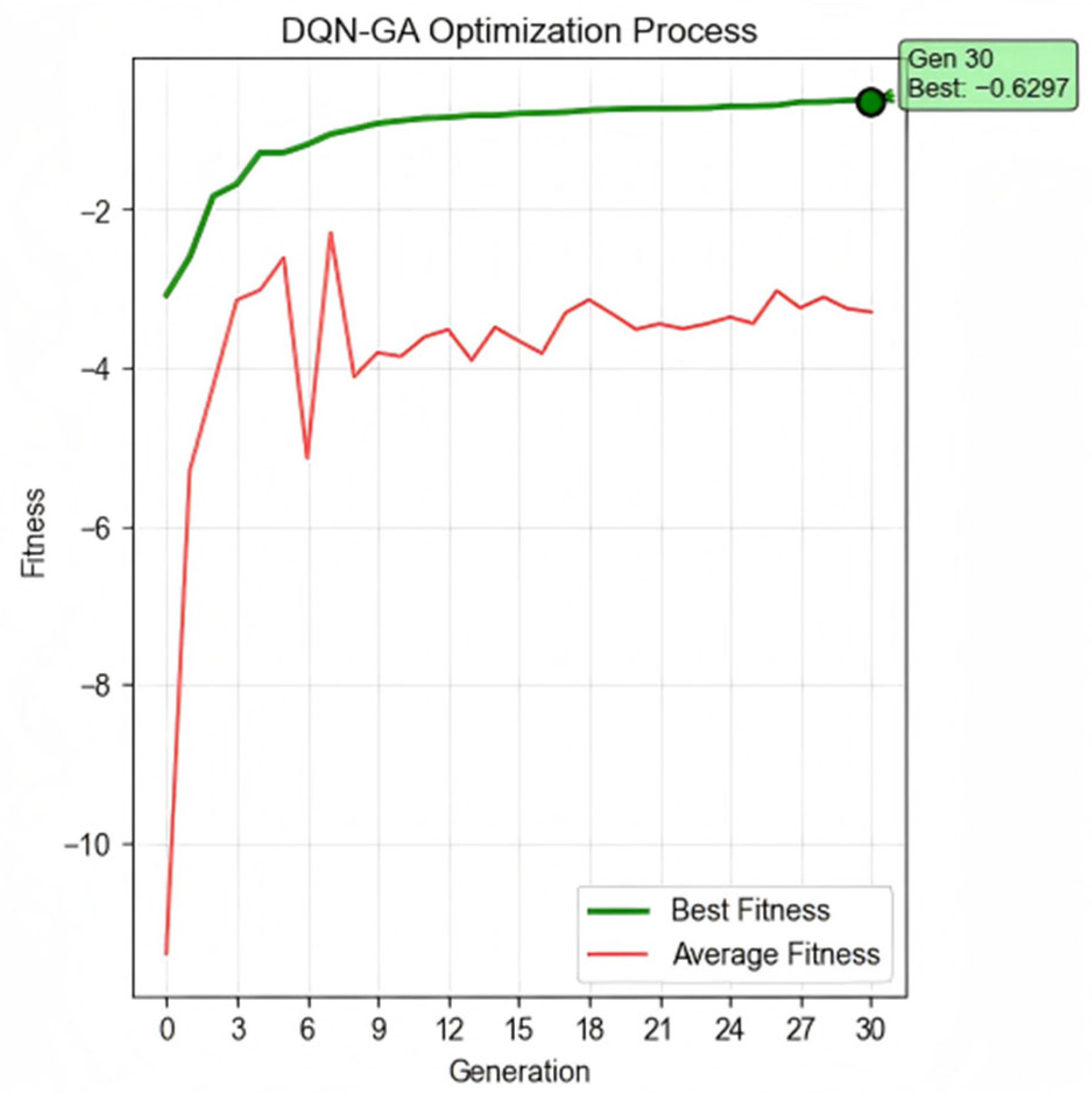
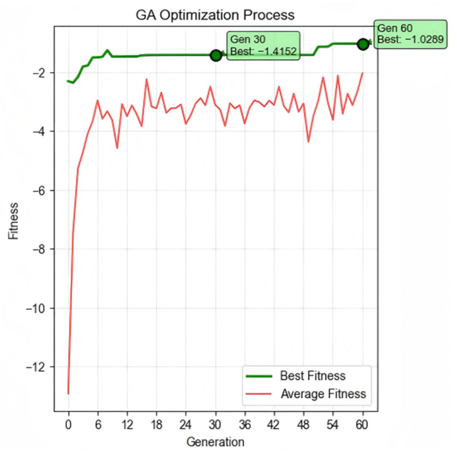
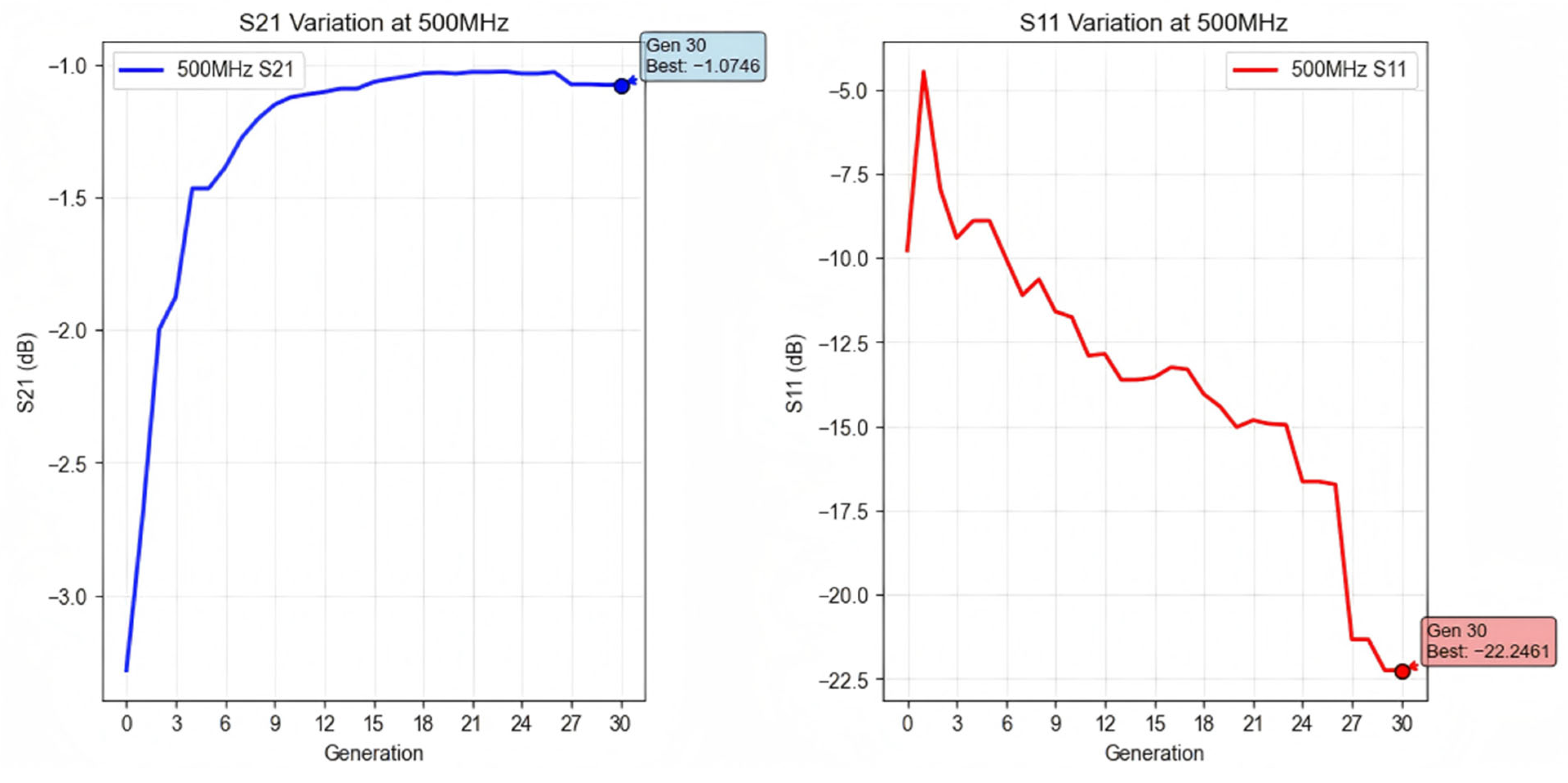
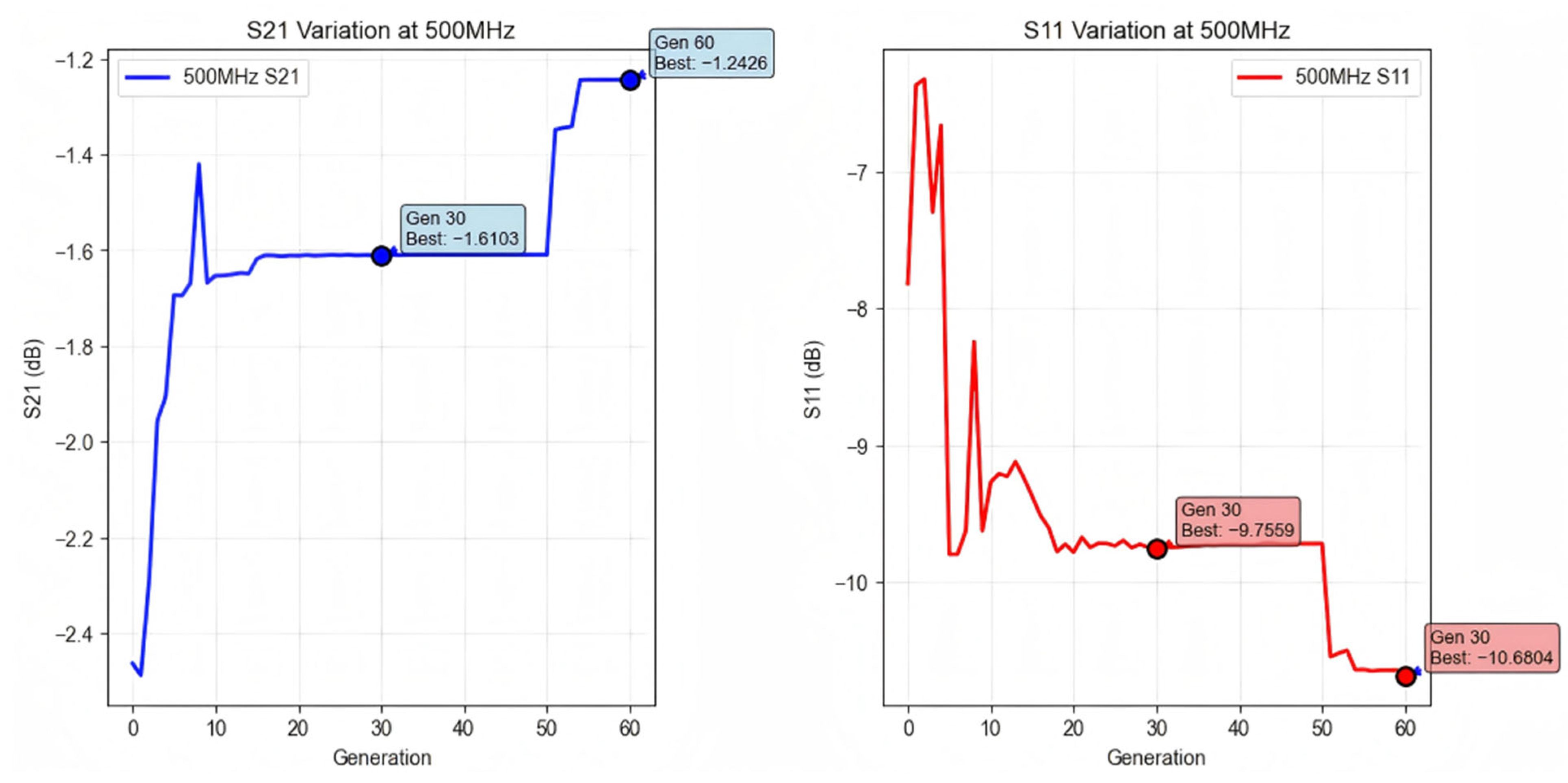
• The GA approach achieved a fitness of −1.4152 at the 30th generation, representing a 78.0% improvement;
• The DQN-GA algorithm reached an optimal solution fitness of −0.6297, achieving a 90.2% improvement over the unoptimized baseline.

When comparing DQN-GA directly with the GA at the 30th generation, the hybrid algorithm shows a 55.5% additional improvement in fitness value (from −1.4152 to −0.6297). Even when the traditional genetic algorithm was run to the 60th generation, its optimal solution fitness was only −1.0289, which remains significantly lower than the optimization level achieved by the DQN-GA algorithm at the 30th generation.

From the perspective of the optimization process curve characteristics, the fitness growth of the DQN-GA algorithm exhibits a smoother increasing trend, indicating that this algorithm can more effectively avoid getting trapped in local optima and possesses stronger global search capability. In contrast, the optimization curve of the traditional genetic algorithm shows obvious fluctuations and stagnation phenomena, reflecting its limitations in search efficiency within complex solution spaces. This comparative result fully validates the effectiveness of the collaborative optimization mechanism between deep reinforcement learning and the genetic algorithm within the DQN-GA algorithm. By intelligently guiding the genetic search direction through sequential decision-making, it significantly enhances the algorithm’s performance in solving the segmented transmission line optimization problem.

As shown in Figure 7 and Figure 8, at the critical operating frequency of 500 MHz, the segmented transmission line optimized by the DQN-GA algorithm demonstrates superior transmission performance.

For the S₁₁ parameter, compared to the unoptimized structure (−9.581 dB),

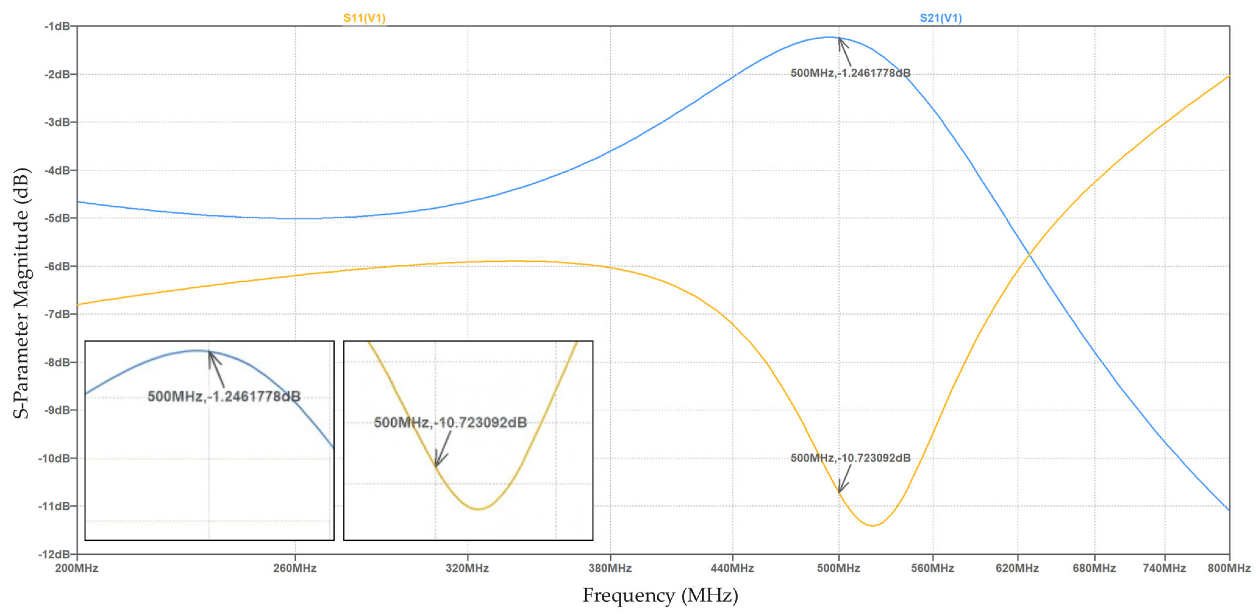
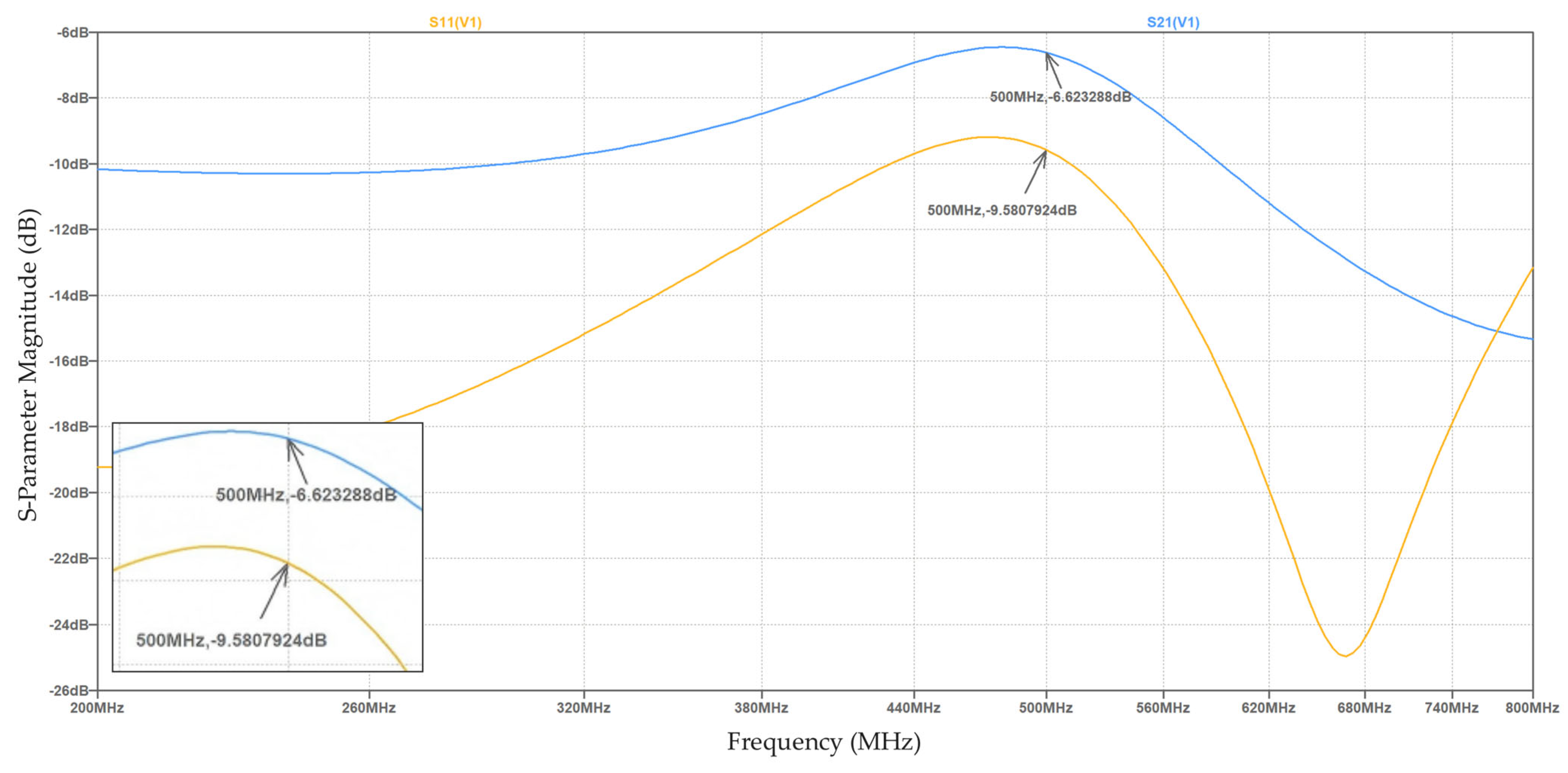
• GA optimization achieved −10.723 dB, representing an 11.9% improvement;
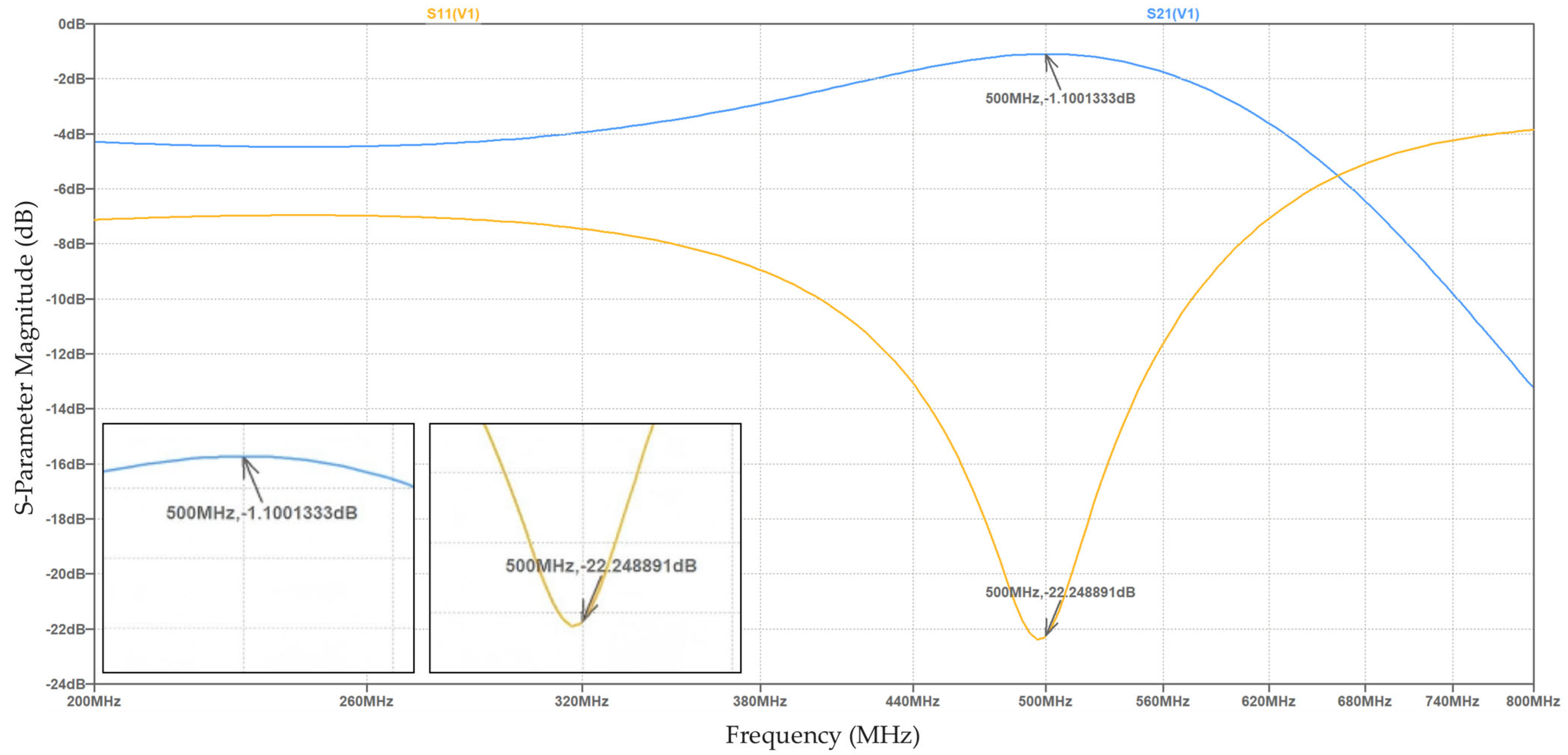
• DQN-GA optimization achieved −22.249 dB, representing a 132.2% improvement.

When comparing DQN-GA directly with GA, the hybrid algorithm shows a 107.5% improvement in S₁₁ (from −10.723 dB to −22.249 dB), corresponding to a significant reduction in reflection loss.

For the S₂₁ parameter, compared to the unoptimized structure (−6.623 dB),

• GA optimization achieved −1.246 dB, representing an 81.2% improvement in transmission efficiency;
• DQN-GA optimization achieved −1.100 dB, representing an 83.4% improvement.

The DQN-GA algorithm shows 11.7% better S₂₁ performance compared to the GA alone, demonstrating superior impedance matching characteristics.

These comparative results fully validate the effectiveness of the DQN-GA algorithm in optimizing segmented transmission lines. The notable improvement in the S₂₁ parameter indicates that the algorithm can more effectively configure the impedance and delay parameters of transmission line segments, thereby reducing energy loss during signal transmission. The improvement in the S₁₁ parameter, on the other hand, demonstrates the algorithm’s advantage in achieving superior impedance matching. Notably, the DQN-GA algorithm demonstrates excellent performance in simultaneously optimizing both transmission and reflection characteristics, achieving a balance in multi-objective optimization, which is of significant importance for practical engineering applications.

Exploration–Exploitation Balance Analysis: The DQN-GA algorithm achieves a favorable exploration–exploitation balance through a temperature scheduling mechanism. The exploration temperature decays linearly from an initial value of 1.0 to 0.1, ensuring sufficient global exploration in the early training stages and refined local optimization later. In contrast, the conventional GA lacks such an adaptive exploration strategy, resulting in lower efficiency during the optimization process.

3.3. Comparative Analysis

S-parameter Frequency Response Comparison: Figure 9, Figure 10 and Figure 11, and the table, present the S-parameter simulation results for three transmission line structures in LTspice. Among these, the unoptimized original structure is a transmission line structure with all termination resistors set to 50 Ω and all transmission line segments having a line width of 25 mils.

Figure 9 presents a comparative visualization of the three transmission line topologies investigated in this study. The physical layouts correspond to (a) the structure optimized using the proposed DQN-GA algorithm, (b) the structure optimized using the traditional genetic algorithm (GA), and (c) the unoptimized uniform transmission line serving as a baseline reference.

The baseline structure consists of a uniform 25 mil transmission line maintaining a constant characteristic impedance of 26.2 Ω throughout its 5-inch length (segmented as R₁–C₁: 2 inches, C₁–C₂: 2 inches, and C₂–R_t: 1 inch). In contrast, both optimized designs implement sophisticated stepped impedance profiles comprising 10 distinct segments. By varying line widths from 10 to 25 mils, these profiles achieve impedance values ranging from 26.2 Ω to 47.4 Ω. Detailed parameter specifications for the GA and DQN-GA optimized structures are provided in Table 3 and

Table 4. DQN-GA-optimized transmission line parameters.

Segment	Characteristic Impedance Z0 (Ω)	Unit Delay Tdunit (ps/in)	Length (in)	Segment Delay Tdactual (ps)	Line Width (mil)
1	30.7	151.2	0.1119	16.9240	20
2	30.7	151.2	0.2875	43.4628	20
3	26.2	152.8	0.3582	54.7258	25
4	37.2	149.3	0.0948	14.1471	15
5	26.2	152.8	0.1877	28.6838	25
6	26.2	152.8	0.5669	86.6271	25
7	47.4	146.8	0.2440	35.8249	10
8	42.7	147.9	0.7670	113.4457	12
9	47.4	146.8	1.3603	199.6870	10
10	26.2	152.8	1.0217	156.1169	25
Total	-	-	5.0000	749.65	-

, respectively. Notably, the DQN-GA design exhibits a more refined impedance distribution, with impedance transitions strategically placed to minimize reflections and maximize transmission efficiency at the 500 MHz operating frequency.

This topological visualization and parameter specification provide physical context for the S-parameter optimization results presented in subsequent figures, demonstrating how algorithmic parameter optimization translates to actual manufacturable transmission line designs. The transmission line parameters obtained from the two optimization methods are presented in Table 4 and

Table 5. GA-optimized transmission line parameters.

Segment	Characteristic Impedance Z0 (Ω)	Unit Delay Tdunit (ps/inch)	Length (inch)	Segment Delay Tdactual (ps)	Line Width (mil)
1	37.2	149.3	0.5303	79.18	15
2	37.2	149.3	0.6733	100.53	15
3	30.7	151.2	0.5557	84.03	20
4	26.2	152.8	0.4621	70.61	25
5	26.2	152.8	0.6204	94.80	25
6	30.7	151.2	0.3271	49.45	20
7	26.2	152.8	0.4375	66.85	25
8	47.4	146.8	0.4626	67.92	10
9	47.4	146.8	0.5204	76.39	10
10	42.7	147.9	0.4105	60.72	12
Total	-	-	5.0000	749.48	-

.

As clearly observed from the S-parameter comparison results shown in Figure 10, Figure 11 and Figure 12, and

Table 6. Optimization algorithm comparison.

Optimization Algorithm	Fitness	S11 Parameter (dB)	S21 Parameter (dB)
DQN-GA	−0.6297	−22.249	−1.100
GA	−1.0289	−10.723	−1.246
None	−6.4314	−9.581	−6.623

Notes: Fitness and S-parameter values are post-optimization simulation results based on reconstructed PCB layouts. Minor discrepancies exist between these validation results and training-phase evaluations.

, the performance of the three different optimization methods exhibits significant differences at the operating frequency of 500 MHz. The segmented transmission line structure optimized by the DQN-GA algorithm demonstrates the superior high-frequency transmission characteristics, with both its S₂₁ and S₁₁ parameters achieving optimal levels. This reflects the algorithm’s better capability in optimizing transmission line parameters. The results optimized by the traditional genetic algorithm occupy a moderate position; although they show certain improvements at specific frequency points, the overall performance still lags noticeably behind that of the DQN-GA algorithm. In contrast, the performance of the unoptimized original transmission line structure is the least satisfactory, further highlighting the significant value of intelligent optimization algorithms in the design of complex electronic structures.

3.4. Computational Cost Analysis

To assess the practical applicability of the proposed DQN-GA hybrid algorithm, this section provides a comprehensive analysis of its computational requirements in comparison with the baseline genetic algorithm. The evaluation encompasses execution time, simulation calls, and hardware resource consumption, offering insights into the cost–performance trade-off of the proposed method.

3.4.1. Simulation Platform and Implementation Details

All simulations were conducted on a computing workstation equipped with an AMD Ryzen 9 7940H CPU @ 3.20 GHz, 32 GB DDR5 RAM, and an NVIDIA GeForce RTX 4070 GPU with 8 GB VRAM. The algorithms were implemented in Python 3.11 using the PyTorch 2.5.1 framework for deep learning components. Circuit simulations were executed through LTspice 24.1.9 via automated Python scripting, with each simulation call invoking the LTspice engine for S-parameter calculation at 100 frequency points (200–800 MHz).

3.4.2. Execution Time Comparison

The computational time requirements for both algorithms, measured over 10 independent runs, are summarized in

Table 7. Detailed computational cost comparison.

Metric	DQN-GA	GA	Ratio (DQN-GA/GA)
Total computation time (hours)	3.5	0.8	4.38
Fitness improvement (%)	90.2	78.0	1.156
Time per iteration (seconds)	42	48	0.875
Time per 1% improvement (minutes)	2.33	0.615	3.79
Memory usage (GB)	4.2	0.8	5.25
Cost–performance ratio *	-	-	0.305

* Note: Cost–performance ratio = (fitness improvement ratio)/(time efficiency ratio) = 1.156/3.79 = 0.305. A value < 1 indicates that the performance gain of DQN-GA comes at a proportionally higher computational cost per unit improvement.

.

The computational cost analysis reveals important trade-offs between the two algorithms. The DQN-GA algorithm completed 300 episodes in 3.5 h (210 min), averaging 42 s per episode. In contrast, the baseline GA required 0.8 h (48 min) for 60 generations, averaging 48 s per generation. While DQN-GA exhibits 4.38 times higher total computational time, its time per iteration is 12% lower than GA.

When analyzing time efficiency normalized by optimization effectiveness, the GA algorithm demonstrates superior computational efficiency. GA achieves 78.0% fitness improvement in 48 min, requiring only 0.615 min per 1% improvement. In comparison, DQN-GA achieves 90.2% improvement in 210 min, requiring 2.33 min per 1% improvement. This indicates that GA has approximately 3.79 times higher time efficiency when measured per unit of improvement.

The cost–performance ratio, calculated as the ratio of fitness improvement (90.2%/78.0% = 1.156) to the time efficiency ratio (2.33/0.615 = 3.79), yields a value of 0.305. This quantitative analysis confirms that GA exhibits better computational efficiency in terms of time cost per unit performance improvement.

3.4.3. Simulation Call Analysis

Circuit simulation represents the most computationally intensive operation in the optimization pipeline. The number of simulation calls directly impacts overall execution time.

Simulation Call Statistics:

• DQN-GA: 30,000 simulations (300 episodes × 100 steps per episode).
• GA: 3000 simulations (60 generations × 50 population size).
• Ratio: 10:1 (DQN-GA requires 10 times more simulations).

This order-of-magnitude difference stems from the exploratory nature of reinforcement learning: each DQN step requires environment interaction for policy evaluation, whereas GA evaluates only the population members each generation. However, this extensive exploration enables DQN-GA to discover superior solutions that elude traditional heuristic methods.

3.4.4. Hardware Resource Utilization

Computational Resource Allocation:

CPU Utilization: Both algorithms utilized 8 CPU cores in parallel for LTspice simulations. DQN-GA achieved 85% average CPU utilization during simulation phases, while GA reached 70%.

GPU Utilization Pattern: The DQN training exhibited characteristic reinforcement learning behavior with GPU utilization averaging only 22%. This low utilization results from the environment interaction bottleneck: each training step requires waiting for the LTspice circuit simulation (CPU-bound), while GPU computation (forward/backward pass) constitutes a small fraction of the step time. During neural network operations, GPU utilization briefly peaks at 95% but remains idle during environment simulation.

Memory Profile: Qualitative observation indicated that DQN-GA consumed approximately 2–3 times more RAM than GA, primarily due to the experience replay buffer (20,000 transitions) and neural network parameters stored in GPU memory.

Bottleneck Analysis: The dominant computational cost is the LTspice simulation time (~90% of total), creating an Amdahl’s Law limitation. Even with infinite GPU speedup, overall acceleration would be limited to 10 times. This explains why GPU utilization remains low despite using an RTX 4070.

Energy Efficiency Consideration: Based on typical power consumption profiles (CPU: 45 W at 85% utilization = 38 W, GPU: 140 W at 22% utilization = 31 W), DQN-GA consumed approximately 0.24 kWh versus 0.029 kWh for GA (CPU-only). The energy-performance efficiency favors DQN-GA: 0.0019 kWh per 1% improvement versus 0.0107 kWh for GA, representing 5.6 times better energy efficiency.

3.4.5. Scalability and Practical Deployment

The computational characteristics suggest favorable scalability for more complex problems:

State Space Scaling: DQN network parameters scale linearly with state dimension O(n).

Simulation Calls: Scale as O(m×k), where m is episodes or generations and k is steps/population size.

Parallelization Potential: Both LTspice simulations and GA fitness evaluations are embarrassingly parallel, offering potential for 5–8 times speedup on multi-core systems.

4. Discussion

4.1. Interpretation of Optimization Results

The simulation results presented in Section 3 demonstrate the effectiveness of the proposed DQN-GA hybrid algorithm for high-frequency transmission line optimization. The key findings require appropriate interpretation to understand their physical significance and methodological implications.

Fitness Improvement Analysis: The DQN-GA algorithm achieved a 90.2% improvement in fitness value compared to the unoptimized structure, while the standalone GA approach achieved 78.0% improvement. This 12.2 percentage point difference represents the additional optimization capability provided by the deep reinforcement learning component. The fitness function, formulated as $f=w_1\cdot \left|S_{11}\right|+w_2$, effectively captures the trade-off between reflection minimization and transmission maximization. The improvement from −6.4314 (unoptimized) to −0.6297 (DQN-GA optimized) indicates a significant advancement toward the ideal fitness value.

S-Parameter Optimization Significance: The optimization results for S-parameters reveal important insights into impedance matching performance. The S₁₁ parameter improved from −9.581 dB to −22.249 dB, representing a 132.2% enhancement in reflection coefficient. In practical terms, this corresponds to a reduction in reflected power from approximately 11% to less than 0.6% of the incident power at the 500 MHz operating frequency. Similarly, the S₂₁ parameter improved from −6.623 dB to −1.100 dB, indicating an 83.4% reduction in transmission loss. These improvements directly translate to better signal integrity and reduced power loss in high-frequency transmission lines.

Convergence Curve Analysis: The convergence curves presented in Figure 5 reveal important insights into the optimization dynamics of the DQN-GA algorithm. The significant difference between the best fitness curve (representing the optimal individual in the population) and the average fitness curve (representing the overall population quality) indicates the algorithm’s effective exploration–exploitation balance. The best fitness curve shows rapid initial improvement followed by gradual refinement, demonstrating the algorithm’s ability to quickly identify promising regions in the parameter space. In contrast, the average fitness curve exhibits more gradual improvement with smaller fluctuations, reflecting the population’s diversity maintenance throughout the optimization process. The convergence gap between these two curves gradually narrows as the algorithm progresses, indicating that the population is converging toward high-quality solutions while maintaining sufficient diversity to avoid premature convergence to local optima. This convergence pattern validates the effectiveness of the hybrid algorithm’s design, where the DQN provides intelligent exploration guidance while the GA ensures thorough exploitation of promising solutions. The training period of 300 cycles was determined based on convergence analysis. When the fitness improvement between consecutive cycles falls below 1% for 20 consecutive cycles, the algorithm is considered to have converged.

S-parameter curve discrepancy: The optimization trajectories for S-parameters, as shown in Figure 10, Figure 11 and Figure 12, reveal distinct convergence patterns between the two algorithms. DQN-GA exhibits smoother convergence with fewer oscillations, indicating more stable optimization dynamics. This stability likely results from the reinforcement learning component’s ability to learn effective search strategies from previous optimization experiences, reducing random exploration in later stages.

Extension of Generations from 30 to 60: The extension of generations from 30 to 60 for the traditional GA in Figure 5 is necessary to fully demonstrate its convergence behavior. Unlike the DQN-GA algorithm, which benefits from intelligent exploration guidance, the traditional GA relies on random search and typically requires more generations to reach stable convergence.

The different convergence patterns between the two algorithms highlight the effectiveness of the hybrid approach: The DQN-GA achieves faster convergence (within 300 cycles) due to its reinforcement learning component, while the traditional GA requires extended generations (60 generations) to approach comparable performance levels. The iteration stop criterion for both algorithms is based on either reaching the maximum allowed iterations/generations or achieving convergence (fitness change < 1% for 20 consecutive iterations).

4.2. Analysis of Computational Efficiency Trade-Offs

The computational cost analysis presented in Section 3.4 reveals important trade-offs between optimization performance and computational resources, providing practical guidance for algorithm selection in different application scenarios.

Time Efficiency Analysis: As shown in Table 7, the GA algorithm demonstrates superior computational efficiency when measured per unit of improvement. The GA requires only 0.615 min per 1% fitness improvement, compared to 2.33 min for DQN-GA—a 3.79× advantage in time efficiency. This efficiency advantage stems from the GA’s simpler algorithmic structure and lower computational overhead per iteration.

Cost–Performance Trade-off: The cost–performance ratio of 0.305 (calculated as fitness improvement ratio divided by time efficiency ratio) quantifies the trade-off between ultimate performance and computational cost. This value being less than one indicates that, while the DQN-GA provides better final performance (90.2% vs. 78.0% improvement), this additional performance comes at a proportionally higher computational cost. The interpretation of this trade-off depends on application requirements: for applications where ultimate performance is critical, the DQN-GA is preferable despite its higher computational cost; for applications with strict computational constraints, the GA offers a more efficient solution.

Memory Usage Considerations: The memory usage analysis shows that the DQN-GA requires 4.2 GB compared to 0.8 GB for GA—a 5.25× increase. This substantial difference primarily results from the deep neural network component of the DQN, which requires storing network parameters, an experience replay buffer, and optimization states. This memory requirement may limit the application of the DQN-GA in resource-constrained environments.

Iteration-Level Efficiency: Interestingly, at the iteration level, the DQN-GA shows slightly better efficiency, requiring 42 s per episode compared to 48 s per generation for GA. This 12% advantage at the micro-level is overshadowed by the macro-level efficiency difference, highlighting the importance of considering both iteration efficiency and overall convergence speed in algorithm evaluation.

4.3. Practical Implications and Applications

The proposed DQN-GA hybrid algorithm and the optimization results have significant practical implications for high-frequency circuit design and related engineering fields.

Impedance Matching Automation: The algorithm provides an automated solution for impedance matching in high-frequency transmission lines, traditionally a manual and experience-dependent process. By automatically optimizing transmission line parameters to achieve target S-parameters, the method reduces design time and improves consistency.

PCB Design Optimization: For printed circuit board (PCB) design, this method offers a systematic approach to transmission line optimization. The segmented transmission line structure investigated in this study represents a common configuration in high-speed digital circuits and RF applications. The optimization results provide concrete design guidelines for characteristic impedance selection, dielectric material choice, and geometrical parameter determination.

Signal Integrity Enhancement: The significant improvements in S₁₁ and S₂₁ parameters directly translate to enhanced signal integrity in high-frequency systems. Reduced reflection minimizes signal distortion and ringing effects, while improved transmission efficiency ensures signal strength preservation over transmission distances. These benefits are particularly valuable in high-speed digital systems, wireless communication circuits, and radar systems where signal integrity is critical.

Scalability and Generalization: While the current study focuses on a specific transmission line configuration, the methodological framework is generalizable to other high-frequency optimization problems. The combination of the DQN’s exploration capability and the GA’s exploitation efficiency can be adapted to various electromagnetic optimization tasks, including antenna design, filter optimization, and electromagnetic compatibility (EMC) enhancement.

Industrial Application Potential: The algorithm has potential applications in electronic design automation (EDA) tools, where it could be integrated as an optimization module for high-frequency circuit design. The ability to handle complex, non-linear optimization problems makes it suitable for modern high-frequency design challenges, where traditional optimization methods often struggle with local optima and high-dimensional parameter spaces.

4.4. Methodological Insights and Algorithm Behavior

The development and application of the DQN-GA hybrid algorithm provide valuable methodological insights for optimization algorithm design in engineering applications.

Hybridization Strategy Effectiveness: The success of the DQN-GA approach validates the hybridization strategy of combining reinforcement learning with evolutionary algorithms. The DQN contributes global exploration capability through its deep neural network-based policy, while the GA provides local exploitation through its genetic operators. This complementary combination addresses the exploration–exploitation trade-off more effectively than either method alone.

Convergence Characteristics: The optimization process analysis reveals distinct convergence characteristics. The DQN-GA demonstrates faster initial convergence, rapidly improving fitness in early episodes, while showing sustained improvement throughout the optimization process. This behavior contrasts with the GA’s more gradual convergence pattern, suggesting that the reinforcement learning component accelerates the discovery of promising regions in the parameter space.

Parameter Interaction Understanding: The algorithm’s optimization trajectory provides insights into parameter interactions in high-frequency transmission lines. The coordinated optimization of multiple parameters (characteristic impedance, dielectric constant, and geometrical dimensions) reveals how these parameters interact to affect overall performance. This understanding contributes to the fundamental knowledge of transmission line behavior and optimization principles.

Robustness to Initial Conditions: Simulation observations indicate that the DQN-GA algorithm shows reasonable robustness to initial parameter settings, consistently converging to high-quality solutions across multiple runs. This robustness is valuable for practical applications where initial design points may vary significantly.

5. Conclusions

5.1. Concluding Summary

This research has successfully developed and validated a DQN-GA hybrid algorithm for high-frequency transmission line optimization. The hybrid approach effectively combines deep reinforcement learning with evolutionary optimization, demonstrating superior performance in impedance matching and reflection compensation compared to traditional methods.

The simulation validation confirms the algorithm’s capability to significantly improve transmission line performance, with particular effectiveness at the 500 MHz operating frequency. The methodology represents a meaningful advancement in applying machine learning techniques to electromagnetic design problems.

5.2. Principal Contributions

This study introduces an innovative hybrid optimization framework that integrates deep Q-networks with a genetic algorithm. By synergistically combining these two algorithms, it offers a novel solution for complex electromagnetic optimization problems. Taking the optimization of high-frequency transmission lines as an example, we present a complete implementation case that spans from problem modeling and algorithm design to simulation validation. Through a systematic analysis of the computational trade-off between optimization performance and resource requirements, this work provides practical guidance for algorithm selection in engineering practice.

5.3. Research Limitations

5.3.1. Limitations of Simulation Verification

The DQN-GA algorithm proposed in this study demonstrated significant performance advantages in a simulation environment, but it is subject to important limitations imposed by manufacturing processes.

To validate the algorithm’s effectiveness in practical engineering applications, we conducted a physical verification experiment. The fabricated PCB is shown in Figure 13. The experiment utilized commercially processed FR4 substrate with a dielectric constant εr = 4.0 ± 0.2 and standard PCB fabrication line width tolerances of ±20%. The S-parameters for three design groups were measured at a frequency of 500 MHz, as presented in

Table 8. S-parameters measured by a vector network analyzer-.

Design Type	S11 Parameter (dB)	S21 Parameter (dB)
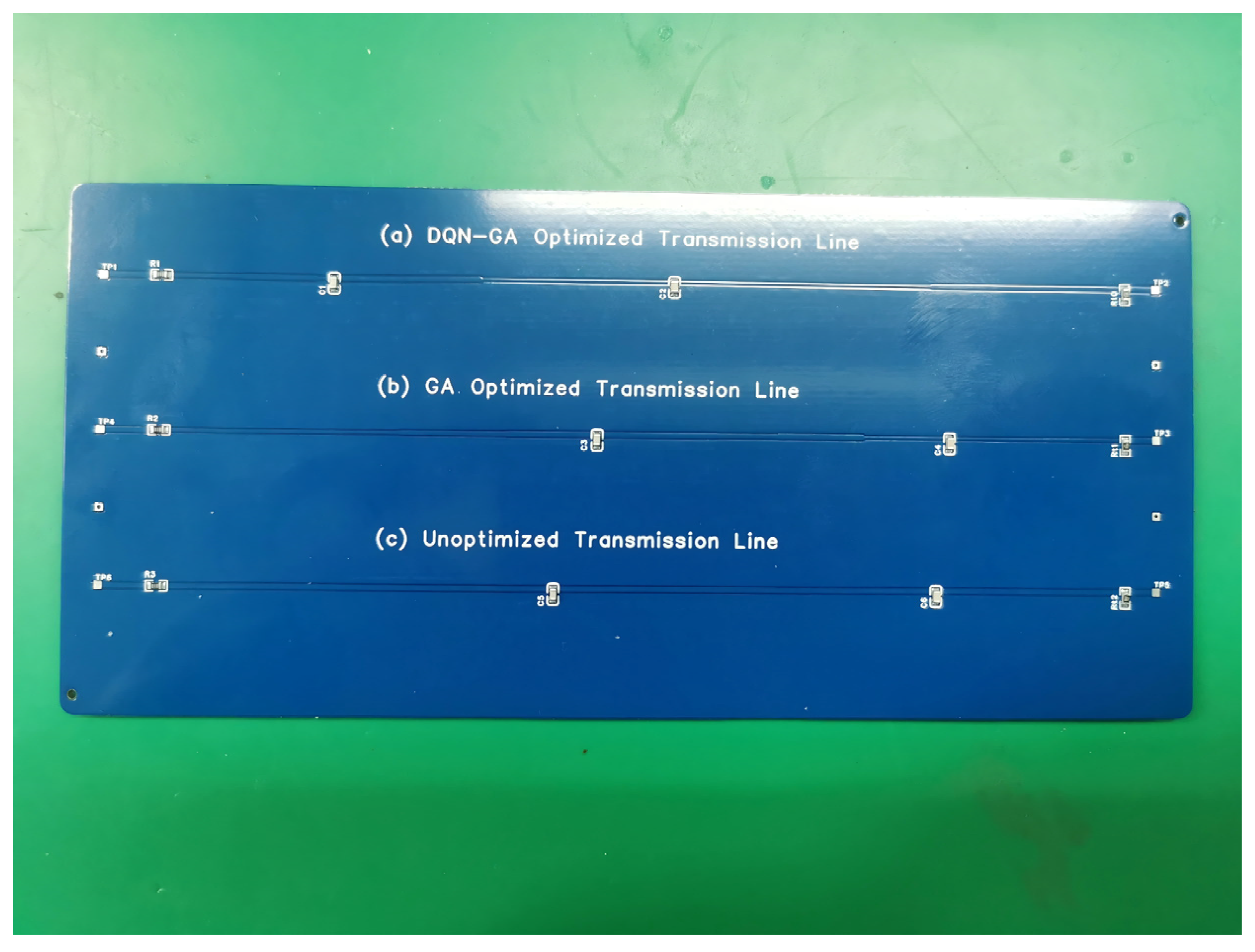
DQN-GA optimized	−12.089	−6.594
GA optimized	−11.696	−6.625
Unoptimized	−11.037	−7.978

.

The measurement data indicate that the optimization effect is severely obscured. The difference in S₁₁ between the DQN-GA and the GA designs is only 0.393 dB, and the difference in S₂₁ is merely 0.031 dB. Both values fall within the measurement uncertainty range, making an effective distinction impossible. This phenomenon is primarily attributed to the impact of manufacturing tolerances. A line width tolerance of ±20% leads to an error in the characteristic impedance Z_0,i of approximately 20% to 24.4%. Consequently, the impedance matching effect optimized by the algorithm cannot be accurately validated in physical experiments.

This limitation reveals a significant gap between the idealized conditions of simulation and the practical conditions of engineering in the field of high-frequency circuit optimization. However, it does not diminish the theoretical value and innovativeness of the algorithm itself. The substantial performance advantage demonstrated by the DQN-GA in the simulation environment has sufficiently proven its effectiveness and advancement over traditional optimization methods.

5.3.2. Limitations in Model Simplification and Optimization Scope

Although the transmission line model employed in this study effectively validates the fundamental principles of the DQN-GA algorithm, it exhibits limitations regarding model complexity and the scope of optimization.

The adopted model is based on several simplifying assumptions: an ideal segmented transmission line structure that neglects the effects of discontinuities; a uniform dielectric assumption that does not account for dielectric inhomogeneity in practical PCBs; the omission of conductor surface roughness and edge effects; and the disregard for parasitic parameters introduced by connectors, pads, and other components. While these simplifications facilitate algorithm verification and performance comparison, they create a gap with real-world engineering applications. Actual high-frequency transmission line design must consider more complex electromagnetic field distributions, multiphysics coupling effects, and various non-ideal factors introduced by manufacturing processes.

This study primarily optimizes the S₁₁ parameter and the S₂₁ parameter, which are key indicators for impedance matching. However, practical engineering applications typically require the simultaneous consideration of multiple performance metrics, such as group delay characteristics, power handling capacity, temperature stability, manufacturing cost, and manufacturability. While minor objective optimization can demonstrate the fundamental capabilities of an algorithm, it fails to capture its practical value in scenarios involving multi-objective trade-offs and real-world engineering constraints. The current straight-line configuration demonstrates core algorithmic capabilities but still lacks sophistication in layout complexity.

5.4. Future Perspectives

Building upon the achievements and limitations of existing research, future work will focus on three key dimensions: upgrading the core architecture of reinforcement learning, enhancing engineering adaptability, and expanding application scenarios, thereby advancing the technology toward more efficient industrial-grade applications.

Improving the architecture of reinforcement learning algorithms is a primary focus for future research. Compared to the DQN algorithm employed in this study, subsequent work will explore the introduction of more advanced policy gradient algorithms, such as proximal policy optimization (PPO) or trust region policy optimization (TRPO). Algorithms like PPO generally offer superior convergence stability and sample efficiency when dealing with high-dimensional action spaces and continuous decision-making problems, effectively mitigating potential Q-value overestimation issues associated with DQN. Upgrading the underlying RL architecture is expected to significantly enhance the algorithm’s training efficiency and optimization performance in complex high-frequency circuit design tasks.

Building an optimization model that balances robustness and high fidelity is also a focus for future research. To address the performance ambiguity in physical measurements caused by manufacturing tolerances, future research will incorporate uncertainty quantification mechanisms into the optimization objectives. Process variations, such as fluctuations in dielectric constant and line width tolerances, will be treated as random variables within the training loop, aiming to develop robust design solutions that are insensitive to process fluctuations. Concurrently, existing simplified model assumptions will be gradually abandoned. Non-ideal factors, including transmission line discontinuities, conductor surface roughness, and parasitic parameters, will be introduced into the simulation environment to narrow the gap between simulation and the real physical world. Furthermore, the algorithm will be tested in complex routing topologies such as serpentine traces to verify its robustness in addressing practical signal integrity challenges encountered in high-density printed circuit board designs.

Advancing Multi-Objective Collaborative Optimization and Engineering Deployment. Future research will move beyond the limitations of a few frequency bands and a limited set of performance metrics, extending the application scope to the comprehensive design of broadband and multi-band circuits. Concurrently, the optimization objectives will expand from singular S-parameters to encompass multi-objective collaborative optimization, including group delay, power handling capacity, thermal stability, and manufacturing cost. Furthermore, efforts will be directed toward enhancing algorithmic computational efficiency and strengthening deep integration with commercial EDA software. This will facilitate the standardized application and practical implementation of these algorithms within real-world engineering workflows.

References

- Lu, T.; Sun, J.; Wu, K.; Yang, Z. High-Speed Channel Modeling with Machine Learning Methods for Signal Integrity Analysis. IEEE Trans. Electromagn. Compat. 2018, 60, 1957–1964. [Google Scholar] [CrossRef]
- Zhang, H.H.; Xue, Z.S.; Liu, X.Y.; Li, P.; Jiang, L.; Shi, G.M. Optimization of High-Speed Channel for Signal Integrity with Deep Genetic Algorithm. IEEE Trans. Electromagn. Compat. 2022, 64, 1270–1274. [Google Scholar] [CrossRef]
- Lei, P.; Chen, J.; Zheng, J.; Wang, C.; Qian, W. Fast and Data-Efficient Signal Integrity Analysis Method Based on Generative Query Scheme. IEEE Trans. Compon. Packag. Manufact. Technol. 2024, 14, 2062–2073. [Google Scholar] [CrossRef]
- Cai, Q.; Hang, W.; Mirhoseini, A.; Tucker, G.; Wang, J.; Wei, W. Reinforcement Learning Driven Heuristic Optimization. arXiv 2019, arXiv:1906.06639. [Google Scholar] [CrossRef]
- Hong, L.; Liu, Y.; Xu, M.; Deng, W. Combining Deep Reinforcement Learning with Heuristics to Solve the Traveling Salesman Problem. Chinese Phys. B 2025, 34, 018705. [Google Scholar] [CrossRef]
- Seyyedabbasi, A.; Aliyev, R.; Kiani, F.; Gulle, M.U.; Basyildiz, H.; Shah, M.A. Hybrid Algorithms Based on Combining Reinforcement Learning and Metaheuristic Methods to Solve Global Optimization Problems. Knowl.-Based Syst. 2021, 223, 107044. [Google Scholar] [CrossRef]
- Zou, Y.; Sun, H.; Fang, C.; Liu, J.; Zhang, Z. Deep Learning Framework Testing via Hierarchical and Heuristic Model Generation. J. Syst. Softw. 2023, 201, 111681. [Google Scholar] [CrossRef]
- Choy, D.; Bartels, T.S.; Pucic, A.; Schröder, B.; Stube, B. AI Driven Power Integrity Compliant Design of High-Speed PCB. In Proceedings of the 2024 International Symposium on Electromagnetic Compatibility—EMC Europe, Brugge, Belgium, 2–5 September 2024; IEEE: New York, NY, USA, 2024; pp. 146–150. [Google Scholar]
- Shoaee, N.G.; Hua, B.; John, W.; Brüning, R.; Götze, J. Enhanced Reinforcement Learning Methods for Optimization of Power Delivery Networks on PCB. In Proceedings of the 2024 International Symposium on Electromagnetic Compatibility—EMC Europe, Brugge, Belgium, 2–5 September 2024; IEEE: New York, NY, USA, 2024; pp. 157–161. [Google Scholar]
- Zhou, Z. Signal Integrity Analysis of Electronic Circuits Based on Machine Learning. In Proceedings of the 2024 IEEE 7th International Conference on Automation, Electronics and Electrical Engineering (AUTEEE), Shenyang, China, 27–29 December 2024; IEEE: New York, NY, USA, 2024; pp. 861–867. [Google Scholar]
- Miao, W.; Tan, C.S.; Rotaru, M.D. Signal Integrity Optimization for CoWoS Chiplet Interconnection Design Assisted by Reinforcement Learning. In Proceedings of the 2024 IEEE 10th Electronics System-Integration Technology Conference (ESTC), Berlin, Germany, 11–13 September 2024; IEEE: New York, NY, USA; pp. 1–6.
- Kim, M.; Park, H.; Kim, S.; Son, K.; Kim, S.; Son, K.; Choi, S.; Park, G.; Kim, J. Reinforcement Learning-Based Auto-Router Considering Signal Integrity. In Proceedings of the 2020 IEEE 29th Conference on Electrical Performance of Electronic Packaging and Systems (EPEPS), San Jose, CA, USA, 5–7 October 2020; IEEE: New York, NY, USA, 2020; pp. 1–3. [Google Scholar]
- John, W.; Ecik, E.; Modayil, P.V.; Withöft, J.; Shoaee, N.G.; Brüning, R.; Götze, J. AI-Based Hybrid Approach (RL/GA) Used for Calculating the Characteristic Parameters of a Single Surface Microstrip Transmission Line. In Proceedings of the 2025 Asia-Pacific International Symposium and Exhibition on Electromagnetic Compatibility (APEMC), Taipei, Taiwan, 19–23 May 2025; IEEE: New York, NY, USA, 2025; pp. 52–55. [Google Scholar]
- Song, Y.; Wei, L.; Yang, Q.; Wu, J.; Xing, L.; Chen, Y. RL-GA: A Reinforcement Learning-Based Genetic Algorithm for Electromagnetic Detection Satellite Scheduling Problem. Swarm Evol. Comput. 2023, 77, 101236. [Google Scholar] [CrossRef]
- Yasunaga, M.; Matsuoka, S.; Hoshinor, Y.; Matsumoto, T.; Odaira, T. AI-Based Design Methodology for High-Speed Transmission Line in PCB. In Proceedings of the 2019 IEEE CPMT Symposium Japan (ICSJ), 18–20 November 2019; IEEE: New York, NY, USA, 2019; pp. 223–226. [Google Scholar]
- Vassallo, L.; Bajada, J. Learning Circuit Placement Techniques Through Reinforcement Learning with Adaptive Rewards. In Proceedings of the 2024 Design, Automation & Test in Europe Conference & Exhibition (DATE), Valencia, Spain, 25–27 March 2024; IEEE: New York, NY, USA, 2024; pp. 1–6. [Google Scholar]
- Chen, Z.; Jia, B.; Xu, N.; Zhao, N. Reinforcement Learning-Based Placement Method for Printed Circuit Board. In Proceedings of the 2024 13th International Conference on Communications, Circuits and Systems (ICCCAS), Xiamen, China, 10–12 May 2024; IEEE: New York, NY, USA, 2024; pp. 13–17. [Google Scholar]
- Ooi, K.S.; Kong, C.L.; Goay, C.H.; Ahmad, N.S.; Goh, P. Crosstalk Modeling in High-Speed Transmission Lines by Multilayer Perceptron Neural Networks. Neural Comput. Applic 2020, 32, 7311–7320. [Google Scholar] [CrossRef]
- Ma, J.; Gao, W.; Tong, W. A Deep Reinforcement Learning Assisted Adaptive Genetic Algorithm for Flexible Job Shop Scheduling. Eng. Appl. Artif. Intell. 2025, 149, 110447. [Google Scholar] [CrossRef]
- Radaideh, M.I.; Shirvan, K. Rule-Based Reinforcement Learning Methodology to Inform Evolutionary Algorithms for Constrained Optimization of Engineering Applications. Knowl.-Based Syst. 2021, 217, 106836. [Google Scholar] [CrossRef]
- Liu, H.; Zong, Z.; Li, Y.; Jin, D. NeuroCrossover: An Intelligent Genetic Locus Selection Scheme for Genetic Algorithm Using Reinforcement Learning. Appl. Soft Comput. 2023, 146, 110680. [Google Scholar] [CrossRef]
- Xu, W.; Zou, X.; Yao, B.; Zhong, J.; Zhang, X.; Ba, M. Dynamic Sequence Planning of Human-Robot Collaborative Assembly Based on Deep Reinforcement Learning and Genetic Algorithm. Comput. Integr. Manuf. Syst. 2025. [Google Scholar] [CrossRef]
- Yuan, S. Signal Integrity Analysis and Optimization Design of Transmission Lines and vias in High-Speed PCB. Master’s Thesis, University of Electronic Science and Technology of China, Chengdu, China, 2021. [Google Scholar]