Article

Real-Time Robotic Navigation with Smooth Trajectory Using Variable Horizon Model Predictive Control

1
School of Teacher Education, Baotou Teachers’ College, Baotou 014030, China
2
School of Department of Electronic and Information Engineering, Shantou University, Shantou 515063, China
3
School of Information and Control Engineering, Southwest University of Science and Technology, Mianyang 621010, China
4
Shenzhen Institute for Advanced Study, University of Electronic Science and Technology of China, Shenzhen 518038, China
*
Author to whom correspondence should be addressed.
These authors contributed equally to this work.
Electronics 2026, 15(3), 603; https://doi.org/10.3390/electronics15030603
Submission received: 11 December 2025 / Revised: 19 January 2026 / Accepted: 27 January 2026 / Published: 29 January 2026

Abstract

This study addresses the challenges of real-time performance, safety, and trajectory smoothness in robot navigation by proposing an innovative variable-horizon model predictive control (MPC) scheme that utilizes evolutionary algorithms. To effectively adapt to the complex and dynamic conditions during navigation, a constrained multi-objective evolutionary algorithm is used to tune the control parameters precisely. The optimized parameters are then used to dynamically adjust the MPC’s prediction horizon online. To further enhance the system’s real-time performance, warm start and multiple shooting techniques are introduced, significantly improving the computational efficiency of the MPC. Finally, simulation and real-world experiments are conducted to validate the effectiveness of the proposed method. Experimental results demonstrate that the proposed control scheme exhibits excellent navigation performance in differential-drive robot models, offering a novel solution for intelligent mobile robot navigation.

1. Introduction

1.1. Motivation

Numerous algorithms have been developed for global path planning and local motion control in mobile robot navigation. The classical global planning methods such as A* [1,2], D* [3], probabilistic roadmap [4] and rapidly-exploring random trees [5] are able to produce collision-free paths in static environments; however, they often ignore the kinematic and dynamic constraints of the robot, which will lead to suboptimal or even unfeasible trajectories when implemented on real robots.
Local navigation techniques such as the dynamic window approach [6], vector field histogram [7,8], artificial potential fields [9], and others [10] provide fast and reactive obstacle avoidance. They struggle with an inherent reliance on user-defined objective function, which can lead to problems including getting caught in local minima, oscillation in close proximity to obstacles, or excessive maneuvers in gregarious environments. Additionally, methods relying on gradient or potential-field approaches, in general, do not consider constraints on inputs and dynamics of the system, which severely limits them when applied in dynamic environments.
Trajectory planners, such as chomp [11] and trajopt [12], find dynamically feasible paths ahead of time but are also prone to issues. These algorithms are usually carried out offline or demand a lot of computing resources, and thus are difficult to implement in real-time on embedded robotic systems.
Instead of relying on the above-mentioned methods, MPC provides a unified optimization framework by integrating robot dynamics, input and state restrictions, and obstacle avoidance goals. This integration enables MPC to generate smoother and safer trajectories, particularly in complex environments such as those discussed in [13,14]. Nevertheless, traditional MPC remains difficult to apply to real-time navigation problems due to its high computational complexity, especially when long prediction horizons are considered.
Choosing the correct prediction horizon for the obstacle avoidance problem presents a significant computational challenge. Specifically, as part of selecting an appropriate prediction horizon, safety, smoothness, and computational burden must all be considered. Existing methods use Control Barrier Functions (CBF) or extend the prediction horizon to ensure safe avoidance of obstacles at all times during navigation [15].
While control barrier functions can benefit from increasing their range for avoiding obstacles, their potential downside is that they may lead to excessively aggressive control actions that will have a negative impact on the predictive controllers’ optimization of trajectory [16]. The expansion of the prediction horizon allows for the opportunity of considering a larger selection of trajectory possibilities, resulting in smoother trajectories than those generated using shorter prediction horizons [17]; however, after reaching a certain level of extension in the prediction horizon, increases in prediction horizon provide diminishing returns in producing smoother trajectories (see Figure 1). In addition to diminishing returns for generating smoother trajectories, excessively long prediction horizons will require the greater computational effort and impair the real-time control performance while decreasing the accuracy of control by introducing model uncertainties and external disturbances [18].
In practical applications, selecting an appropriate length of a prediction horizon represents a major challenge since the decision is predicated upon weighing a number of competing concerns. A shorter prediction horizon when navigating the robot provides a higher quality of control performance while the robot is traveling far from any obstacles; however, when the robot approaches obstacles, a longer prediction horizon will be more effective in providing adequate levels of safety, as well as generating smoother trajectories. Hence, dynamically selecting a changing distance to an obstacle based upon the robot’s point-of-view dynamically provides an increase in the robot’s real-time control performance and trajectory smoothness, both of which could be accomplished through a dynamically selected prediction horizon [19]. To address this issue, we have developed a variable prediction horizon approach to model predictive control, adapting to the distance between the robot and any nearby obstacles to create a balance of safety and real-time control performance, improving navigation.

1.2. Related Work

1.2.1. Model Predictive Control

Recent advances in navigation have allowed MPC to produce a variety of beneficial outcomes, including [20,21,22]. MPC uses an optimization approach where control inputs are determined based on how they will affect the future state of the system over the fixed prediction horizon, allowing MPC to incorporate and account for the constraints imposed by the system and any dynamic changes occurring to the operational environment. As such, there are numerous examples of the application of MPC technology to many aspects of autonomous vehicles and robotic navigational tasks. However, as the complexity of robotic systems and operational environments continues to rise, so too does the resultant potential for increased computational complexity, decreased real-time performance and increased safety issues associated with MPC [23].
Obstacle avoidance can be achieved through a variety of methods, including the dynamic window approach [6], collision-free flight corridors [24,25], artificial potential fields [9], gradient maps [26], and others [27]. However, these methods may not be effective in more challenging scenarios. Obstacle avoidance can also be implemented using MPC, and when control barrier functions are applied, they can help the robot avoid obstacles at greater distances [15,28]. Nevertheless, MPC may sometimes be conservative. To address this issue, we employ a longer prediction horizon in MPC to satisfy the obstacle avoidance objectives.
Another challenge is the speed of solving the MPC optimization. Initially, single shooting methods were used to solve the problem [29,30], but as the problem grew, the solving speed slowed down. To tackle this, multiple shooting methods were introduced [31,32,33]. Additionally, using a warm start [34] can speed up the solving process. In this study, we improve the warm start initial guess for cases with variable prediction horizons.

1.2.2. Multi-Objective Evolutionary Algorithm

As the complexity of optimization problems increases, traditional single-objective optimization methods often fail to meet the practical demands when dealing with multi-objective optimization problems. In multi-objective optimization, there are typically conflicts or trade-offs between objectives, so finding a set of Pareto optimal solutions becomes key to solving such problems [35]. Multi-objective evolutionary algorithms have gained widespread attention due to their advantages in solving non-convex, multiple objective optimization problems. Unlike traditional optimization methods, multi-objective evolutionary algorithms simulate the process of natural selection through evolutionary strategies, continuously evolving a set of effective multi-objective solutions from a population using operations such as fitness evaluation, selection, crossover, and mutation. There are several types of multi-objective evolutionary algorithms, including dominance-based [36], decomposition-based [37], and indicator-based algorithms [38].
Among the various multi-objective evolutionary algorithms, the non-dominated sorting genetic algorithm II (NSGA-II) [39] stands out as one of the most representative and widely used algorithms due to its efficiency and good convergence properties. The NSGA-II algorithm employs a domination-based sorting method, retaining high-quality solutions through an elitism strategy, and maintains solution diversity using a crowding distance measure. By performing non-dominated sorting, the algorithm divides the population into multiple levels, effectively avoiding the “premature convergence” problem seen in traditional genetic algorithms, while also achieving a good balance among multiple objectives. In this study, we will use the NSGA-II algorithm to obtain the optimal control parameters.
Although NSGA-II has been widely used for tuning MPC parameters such as weighting matrices, existing studies mainly focus on adjusting Q and R under a fixed prediction horizon. For example, Qazani et al. [40] optimized MPC weights for autonomous vehicles, and Arshad et al. [41] applied NSGA-II to tune torque-control weighting factors. However, very few works address the optimization of the prediction horizon itself, which is a discrete parameter closely coupled with computational burden, real-time constraints, and navigation performance. This makes horizon optimization significantly more challenging than weight tuning. Therefore, instead of jointly tuning all parameters, this work concentrates on NSGA-II-based optimization of the prediction horizon for real-time navigation MPC.

1.3. Contribution

The contributions of this study are summarized as follows:
  • We propose a variable prediction horizon model predictive control scheme based on the change in obstacle distance to improve trajectory smoothness and real-time performance during navigation.
  • We combine the multi-objective evolutionary algorithm NSGA-II with model predictive control to obtain optimal parameters and achieve better control performance. Compared with traditional weight parameter adjustment methods, we mainly focus on optimization in the prediction horizon.
  • We validate the effectiveness of the proposed method in balancing real-time performance and trajectory smoothness through both simulation experiments and real-world scenario testing.

2. Preliminaries

2.1. System Model

In Model Predictive Control, the establishment of an accurate system model is crucial. In this study, we adopt a differential drive robot model, which is described as follows:
x ˙ = v cos θ y ˙ = v sin θ θ ˙ = ω ,
where x, y, and  θ represent the robot’s x-coordinate, y-coordinate, and orientation with respect to the x-axis, respectively. The control inputs v and ω represent the linear velocity and angular velocity inputs, respectively. It is important to note that, for modeling accuracy, we discretize the system using the explicit Runge–Kutta method.
Let X = x , y , θ T and U = v , ω T . The discrete time control system is defined as:
X t + 1 = f X t , U t ,
where f X t , U t is the system’s dynamics function at time step t. The MPC planning problem can be formulated as:
J t ( X t , U t ) = min U t : t + N 1 | t p ( X t + N | t ) + k = 0 N 1 q ( X t + k | t , U t + k | t )
s . t . X t + k + 1 | t = f ( X t + k | t , U t + k | t ) , k = 0 , , N 1
X t + k | t X , U t + k | t U , k = 0 , , N 1
X t | t = X t
X t + N | t X f
g X t + k | t 0 , k = 0 , , N 1
where N represents the prediction horizon, X t + k | t denotes the state vector at time t + k predicted from time t, and  X , U , X f represent the state constraints, control constraints, and terminal set, respectively. p and q represent the terminal cost and stage cost, respectively. The function g captures the obstacle avoidance constraints, which can be formulated using conventional obstacle avoidance constraints.

2.2. Multiple Shooting

In standard MPC, the control strategy is typically derived by solving an optimization problem with system dynamics constraints. In a multi-step optimal control problem, control inputs are typically optimized over a future time horizon. This involves optimizing a cost function subject to system dynamics constraints, often resulting in a nonlinear optimization problem that can be complex to solve.
Multiple shooting [31,32] is a technique that has shown to reduce computational load, as well as improve the ability to solve problems, through splitting up optimization problems into smaller subproblems. This concept is based on breaking the integrative process into small segments in time. Control action predictions of the next N intervals are treated as a component of the optimization variables and multiple shooting uses the system model as a state constraint at each optimization step.

2.3. Warm Start

Warm start [34] in the context of an optimization problem addresses the inefficient use of available resources in producing a final solution. The warm-start technique can be used over multiple iterations, where a portion of the solution from the previous iteration serves as a reference for the subsequent iteration. For real-time performance, warm starting an optimization procedure accelerates convergence to an effective solution, thereby reducing the computational time per iteration.

3. Implementation

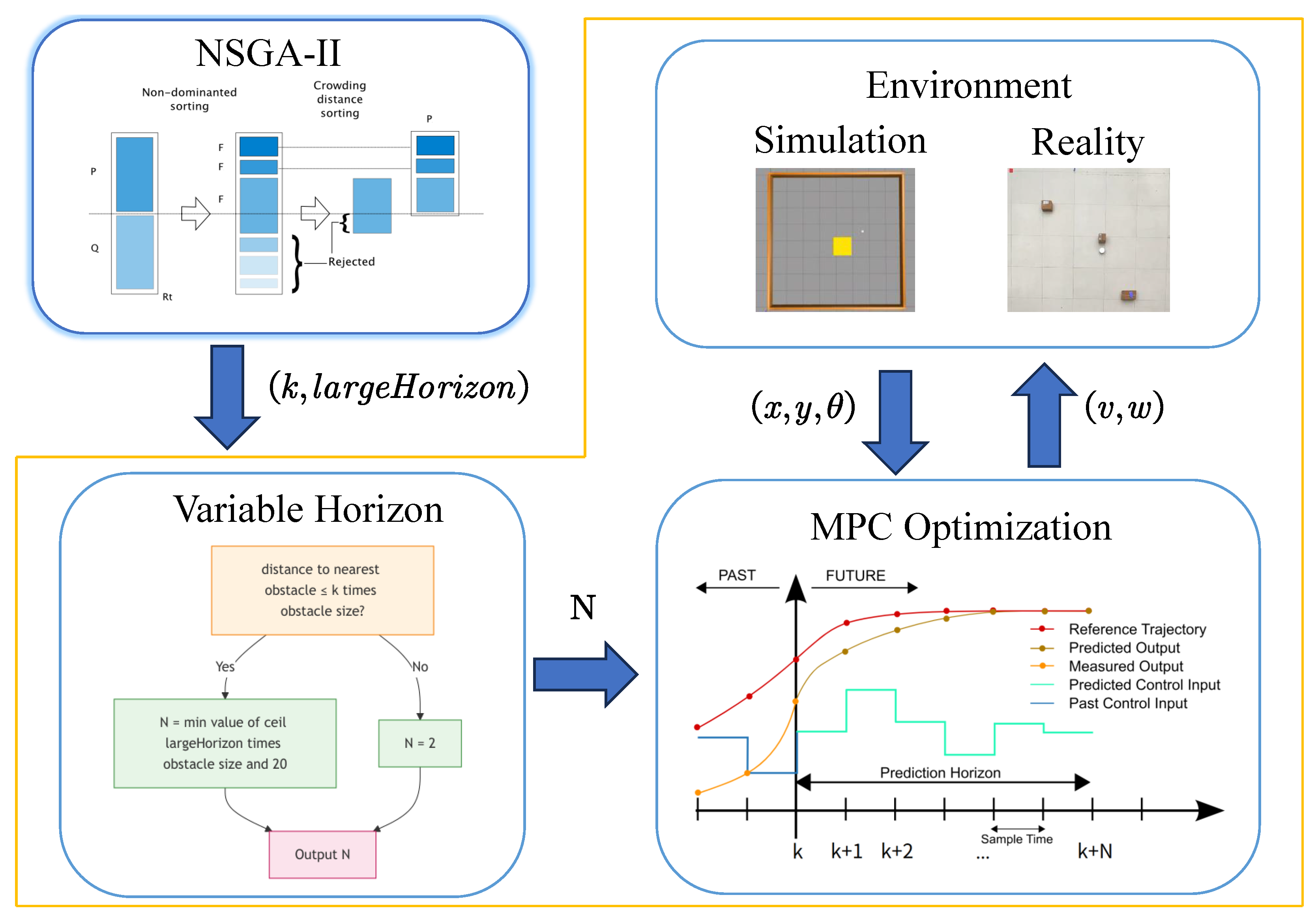
The overall framework of the proposed variable horizon model predictive control strategy based on multi-objective evolution algorithm is shown in Figure 2.

3.1. Variable Prediction Horizon Control Scheme

When approaching obstacles, a longer prediction horizon can help avoid obstacles more effectively and generate smoother trajectories. However, if the prediction horizon is always long, the real-time performance is relatively low. Therefore, this study adopts a variable prediction horizon scheme. Specifically, when the robot is within k s i z e ( o b s ) m of an obstacle and moving toward it, a larger prediction horizon is used; when the robot is farther than k s i z e ( o b s ) m from the obstacle, a smaller prediction horizon is employed. Here, k is a positive coefficient, and s i z e ( o b s ) represents the size of the obstacle. This reflects that, as the size of the obstacle increases, a larger prediction horizon should be switched to at a greater distance. Additionally, the prediction horizon should adapt based on the size of the obstacle. To achieve simplicity, the prediction horizon upon departing from the obstacle is defined to be 2; the maximum prediction horizon permitted by the model is 20. The specific implementation of the method of dynamically adjusting a prediction horizon is described in Algorithm 1. In this algorithm, k is a positive constant which identifies the base distance for an expanded prediction horizon when the size of the obstacle is 1 m. When the obstacle is of a larger or smaller dimension than 1 m, the threshold distance is scaled according to the total size of the obstacle. The parameter l a r g e H o r i z o n determines the base prediction horizon size once expansion is triggered for a 1 m obstacle. For obstacles of varying sizes, the expanded horizon scales proportionally to s i z e ( o b s ) , resulting in a larger horizon for larger obstacles.
To provide for simplicity and to achieve rapidity of response to the obstacles, the prediction horizon when departing from an obstacle is defined to be 2. This minimum prediction horizon guarantees that the model predictive control system predicts two future states, which is sufficient for feasible trajectory generation without placing excessive computational demands on the system. The highest prediction horizon of 20 is based on empirical findings from simulation experiments, as illustrated in Figure 1, indicating that all trajectory data produced by prediction horizons close to 20 are virtually identical, suggesting that increasing the prediction horizon indefinitely would yield diminishing returns on the predictability of future trajectories, and further prediction horizons would create increased computational costs and lower real-time capabilities. Hence, a maximum prediction horizon of 20 provides a reasonable balance between control performance and computational efficiency.
As shown in Algorithm 1, once the real-time distance to the obstacle and the size of the obstacle are known, we can determine the size of the prediction horizon and dynamically adjust it. In fact, the maximum prediction horizon does not necessarily need to be 20; it is generally determined based on the robot’s speed, computational efficiency, and other factors. Similarly, the minimum prediction horizon does not necessarily need to be 2, but typically, the smaller the prediction horizon, the higher the real-time performance. Therefore, when the robot is not close to the obstacle, a prediction horizon of 2 is generally chosen.
Algorithm 1 Variable Prediction Horizon Scheme
1:
Output: N
2:
Input:   d i s t T o O b s t a c l e , s i z e ( o b s ) , l a r g e H o r i z o n , k
3:
if   d i s t T o O b s t a c l e k ×   s i z e ( o b s ) and approaching the obstacle  then
4:
    N min l a r g e H o r i z o n × s i z e o b s , 20
5:
else
6:
   N 2
7:
end if
As mentioned earlier, multiple shooting and warm start are both techniques used to accelerate the optimization process in MPC solving. The variable horizon scheme is implemented within a multiple shooting framework, where shooting intervals are dynamically added/removed according to the adjusted prediction horizon. a warm start uses the solution from the previous optimization problem as the initial guess for the current optimization problem, which can speed up the solving process and improve real-time performance in control. However, when the prediction horizon changes, the prediction horizon from the previous optimization problem may not align with the prediction horizon at the current time step. To address this, we propose a simple solution.
When the current prediction horizon is shorter than the previous one, the initial guess is taken as the front part of the previous solution. When the current prediction horizon is longer than the previous one, the initial guess is taken as the entire previous solution, extended by the last solution.
This approach ensures that the warm start can still be effectively applied, even when the prediction horizon changes, allowing for faster and more efficient optimization.

3.2. Optimal Control Parameter Selection

In this study, we use the NSGA-II algorithm to obtain the optimal parameters k and l a r g e H o r i z o n for Algorithm 1. The optimal parameters are obtained by using a multi-objective optimization approach to achieve better control performance. To evaluate the real-time performance and safety of the navigation process, we use two metrics: the number of optimization problem solutions divided by the total time, and the distance between the entire trajectory and the obstacles. Since NSGA-II’s objective functions generally aim to minimize values, and the two metrics mentioned above are better when larger, the following function is used as the final evaluation function for NSGA-II:
r e a l T i m e F u n = C 1 m p c i t e r t o t a l T i m e ,
s a f e F u n = exp C 2 · d i s t a n c e + C 3 .
Here, C 1 , C 2 , and  C 3 are positive constants, with  C 1 = 200 , C 2 = 8 , and  C 3 = 2 specified. In this context, m p c i t e r represents the number of optimization problems solved during the navigation process, t o t a l T i m e is the total navigation time, and  d i s t a n c e refers to the distance from a point on the trajectory to the obstacle. With this design, the two evaluation function metrics are minimized, leading to improved navigation performance.
In order to implement the NSGA-II algorithm successfully, a number of methods are used in conjunction with tournament selection to determine the dominant parents of a population based upon the crowding distance and dominance levels of these parents. Following the selection of parents, the new offspring generated via simulated binary crossover between the selected parents, which takes into account both the parent’s decision variable ranges as well as their strengths, are created. The next step is to perform a polynomial mutation on the generated offspring to ensure the offspring’s genotype will remain within viable bounds post-mutation. Finally, all offspring are subjected to non-dominance sorting to establish a ranked order of descendants and select the best performing individuals to continue the evolution of the population. The detailed process of using NSGA-II to obtain the optimal variable prediction horizon control parameters can be found in Algorithm 2.
Algorithm 2 NSGA-II Based Adaptive Horizon MPC Parameter Optimization
  1:
Output: k, l a r g e H o r i z o n
  2:
Input: NSGA-II parameters (population size, max iterations, etc.), MPC parameters (prediction cycle, etc.)
  3:
Step 1. Initialize parameters: Initialize NSGA-II and MPC parameters
  4:
Step 2. Generate the initial population: Randomly initializing individuals (k, l a r g e H o r i z o n ) within variable constraints
  5:
Step 3. MPC Simulation Evaluation: Solve the MPC optimization problem for each individual using Algorithm 1
  6:
Step 4. Compute objective functions:   r e a l T i m e F u n and s a f e F u n
  7:
Step 5. Non-dominated sorting: Perform Pareto ranking based on the objective functions
  8:
Step 6. Compute crowding distance: Calculate the solution distribution density within the same Pareto front
  9:
Step 7. Evolutionary operations: Tournament selection, simulated binary crossover, polynomial mutation
10:
Step 8. Environmental selection: Merge parent and offspring populations, retaining the best individuals
11:
Step 9. Termination check: If max iterations are reached, plot the Pareto front; otherwise, return to Step 3
12:
Step 10. Deploy optimal solution: Select the best (k, l a r g e H o r i z o n ) combination from the Pareto front that balances real-time performance ( r e a l T i m e F u n ) and safety ( s a f e F u n )

4. Experiments

In this section, both simulation and real-world experiments are used to validate the effectiveness of our proposed variable horizon model predictive control scheme. The optimization problem is solved using CasADi [42] and the IPOPT solver [43].

4.1. Simulation Scenario

Firstly, we use the NSGA-II algorithm to determine the appropriate parameters. During the training of optimal parameters, a single obstacle is used for navigation training. The starting position is [ x , y ] = [0 m, 3 m], and the destination is [7 m, 7 m]. The initial and final orientations are both set to 0 rad. And the prediction cycle for solving the optimization problem is 0.1 s. The obstacle is a 1 × 1 m2 square with its center located at [3.5 m, 4.5 m]. The maximum allowable speed of the robot is 0.5 m/s and the safety collision radius is set to 0.2 m. The stage cost and terminal cost in (3) are set as follows:
q X k , U k = X k Q X k + U k R U k , p X N = X N P X N ,
where Q = 10 I 3 with Q 3 , 3 = 0.1 ; R = 0.5 I 2 , with R 2 , 2 = 0.05 ; P = 1000 I 3 , with P 3 , 3 = 1 .
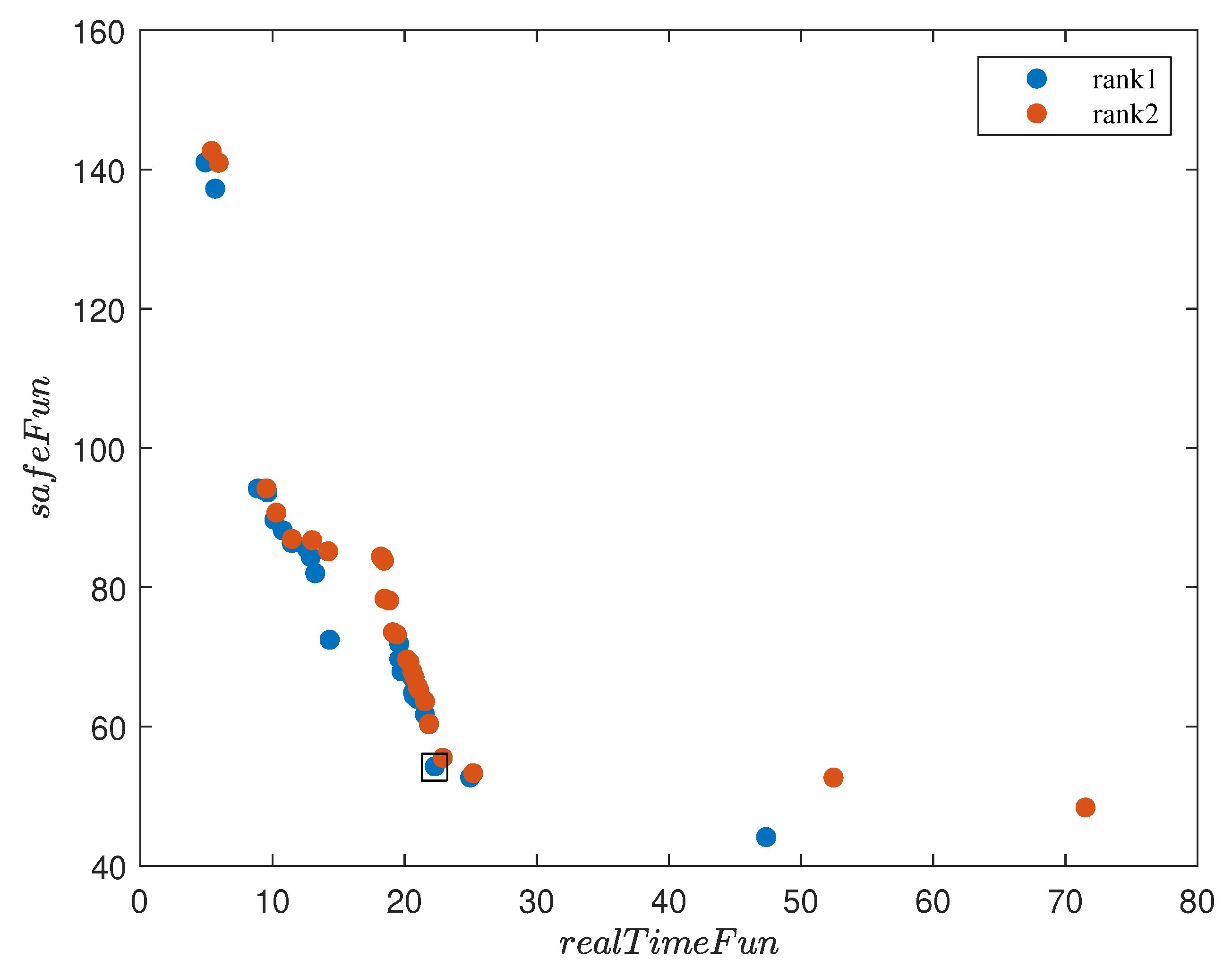
The range of the optimization variable l a r g e H o r i z o n is set from 2 to 20. This range was chosen because a horizon smaller than 2 provides insufficient prediction for safe navigation, while horizons larger than 20 offer little improvement in trajectory smoothness but reduce real-time performance. The range of k is set from 0.2 to 3, which defines the base distance at which horizon expansion begins. For obstacles of different sizes, the threshold distance naturally scales according to s i z e ( o b s ) . Therefore, setting the base obstacle avoidance distance of our robot to the range of 0.2 to 3 m is reasonable. In the NSGA-II algorithm, a population size of 50 is used, and a total of 200 generations are iterated. The crossover probability is set to 1, the mutation probability is set to 0.4, the crossover distribution index is set to 2, and the mutation distribution index is set to 5. The NSGA-II algorithm parameters, including population size, number of generations, crossover/mutation probabilities, and distribution indices, are set according to commonly used standard values in evolutionary algorithms. The final Pareto front obtained is shown in Figure 3. In principle, all rank-1 solutions on the Pareto front are feasible candidates. However, in practical implementation, safety considerations are prioritized. Specifically, Pareto-optimal solutions for which the safety-related objective s a f e F u n remains below a predefined threshold (e.g., s a f e F u n < 60) are first identified. Among these safety-feasible solutions, the one with better real-time performance is selected. Following this criterion, the chosen Pareto solution corresponds to k = 0.9 / 2 and l a r g e H o r i z o n = 16 / 2 . This scaling is applied because the obstacle size used in the NSGA-II optimization scenario is 2 m. Accordingly, when the obstacle size is 2 m, the prediction horizon is set to 16 once the robot enters the corresponding distance threshold and moves toward the obstacle.
Although the parameters k and l a r g e H o r i z o n were optimized in a simplified single-obstacle scenario, they are intended to capture the general characteristics of the proposed variable prediction horizon adaptation mechanism rather than being tailored to a specific environment. The following experiments were conducted in more complex scenarios with multiple obstacles of different sizes and configurations. These experiments show that the same parameter set is still effective, indicating a reasonable level of generalization beyond the optimization scenario.
We performed the optimization using NSGA-II with a population size of 50 individuals across 200 generations using a standard desktop computer identified as an Intel i5-12500 CPU with 16GB RAM. The optimization process was run for approximately 56 h, generating a total of 10,050 objective function evaluations. It should be noted, however, that the overhead associated with this computation will only have to be performed one time. Although the optimization performed offline has a heavy computational requirement, the results generated (values for k and l a r g e H o r i z o n ) will not have to be recomputed each time an online navigation task is conducted.
The computer used for the simulation has an Intel i5-12500 CPU and an Intel UHD Graphics 770 GPU. To evaluate the performance of the proposed method, we compare it with fixed-horizon MPC by using prediction horizons of 2, 10, and 20. The simulation scenario is expanded to include three obstacles, with the starting position set to [1 m, 1 m], while all other settings remain unchanged. The first and third obstacles are confined within the x-y intervals [2 m, 3 m] × [3 m, 4 m] and [5.3 m, 5.8 m] × [5.5 m, 6.5 m]. The midpoint of the second circular obstacle is [5 m, 4 m] and the radius is 0.5 m.
To evaluate the advantages of the proposed variable prediction horizon MPC method, we also compared it with the CBF-MPC method [15,44]. The latter is a typical safety-aware MPC strategy and a fixed prediction horizon of N = 10 is used.
In CBF-MPC, there is a relaxation factor γ [ 0 , 1 ] . In our experiment, γ was set to 0.3 because when γ is too small, it often leads to overly conservative behavior, resulting in larger obstacle avoidance deviations and less smooth trajectories. When γ is equal to 1, it behaves the same as regular MPC.
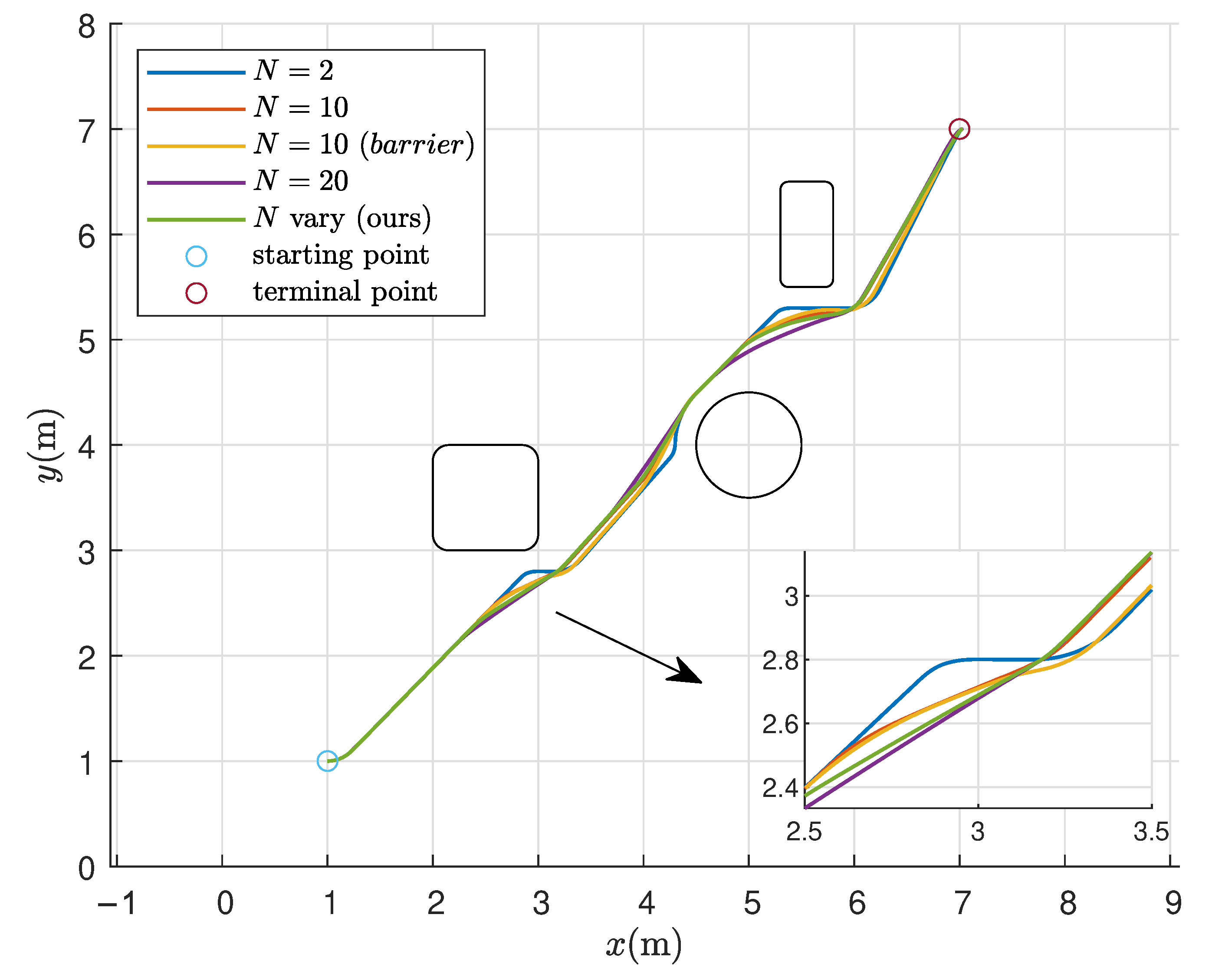
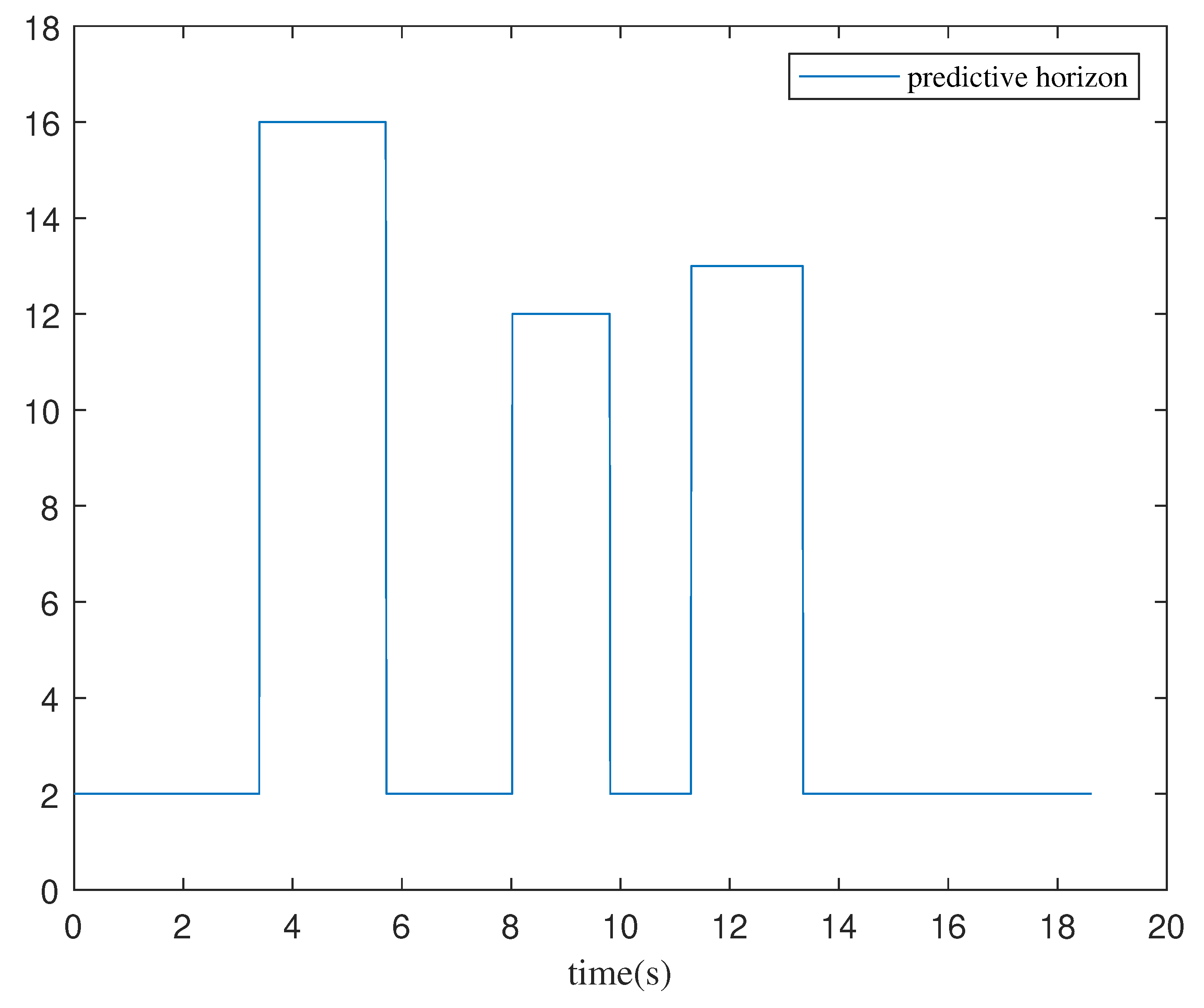
The resulting trajectory plots are shown in Figure 4, while Figure 5 illustrates the variation of the prediction horizon over time. From Figure 4, it can be observed that the trajectory generated by the proposed method is close to that obtained using a fixed prediction horizon of 20, indicating that the proposed approach preserves good trajectory smoothness. The trajectories produced by MPC with CBF and MPC without CBF follow similar overall paths in this scenario, although differences can be observed in terms of safety margins and trajectory regularity.
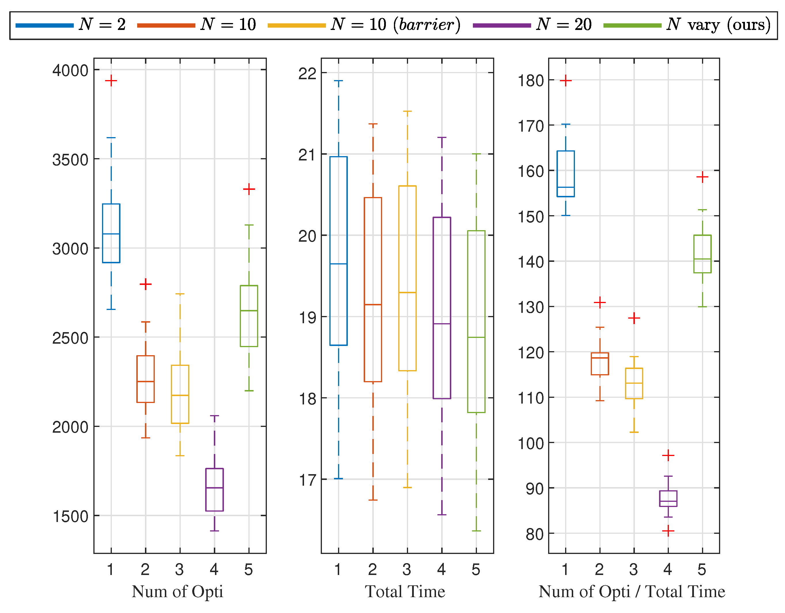
Furthermore, as shown in Figure 4 and Figure 5, when encountering obstacles of different sizes and shapes, the proposed algorithm is able to adaptively adjust its prediction horizon during navigation. In addition, 19 further experiments were conducted with randomly generated starting positions within 0 < x < 2 and 0 < y < 2 . The total number of optimization steps and the total navigation time were recorded, and their ratio was used to compute the average number of optimizations per second. In total, 20 experiments were performed, and the statistical results are summarized in the box plot below. Here, “Num of Opti” and “Total Time” denote the total number of optimization steps and the total navigation time, respectively. The averaged results are reported in Table 1.
As shown in Figure 6 and Table 1, as the prediction horizon increases, the number of optimization solutions decreases, and real-time performance deteriorates. In the third subplot of Figure 6 and Table 1, it can be seen that our proposed method does not degrade real-time performance much compared to the case with a prediction horizon of 2.
Furthermore, the figure shows that the CBF-based MPC ( N = 10 ( b a r r i e r ) ) exhibits slightly lower real-time performance compared to the standard MPC without CBF ( N = 10 ) at the same horizon. This can probably be explained by the fact that additional CBF optimization in every optimization step costs more time.
To quantitatively measure the smoothness of a trajectory, we consider the root mean square (RMS) curvature of the trajectory as a scalar measure. Curvature is used to quantify the bending of the trajectory at each point, and the RMS value summarizes the overall curvature along the trajectory. The curvature at a point on the trajectory, in terms of the position coordinates ( x , y ) , is given by
κ = | x y y x | ( x 2 + y 2 ) 3 / 2 ,
where x and y are first derivatives, and x and y are second derivatives with respect to the trajectory parameter (e.g., arc length or index). When discrete trajectory points are used, numerical differentiation is applied, and points that are too close together (i.e., with a Euclidean distance smaller than 0.001) are filtered out to avoid numerical instability. The RMS curvature is then computed as
RMS κ = 1 M i = 1 M κ i 2 ,
where M is the number of valid points. A smaller RMS curvature indicates a smoother trajectory, making this metric suitable for comparing the smoothness of trajectories generated under different control strategies.
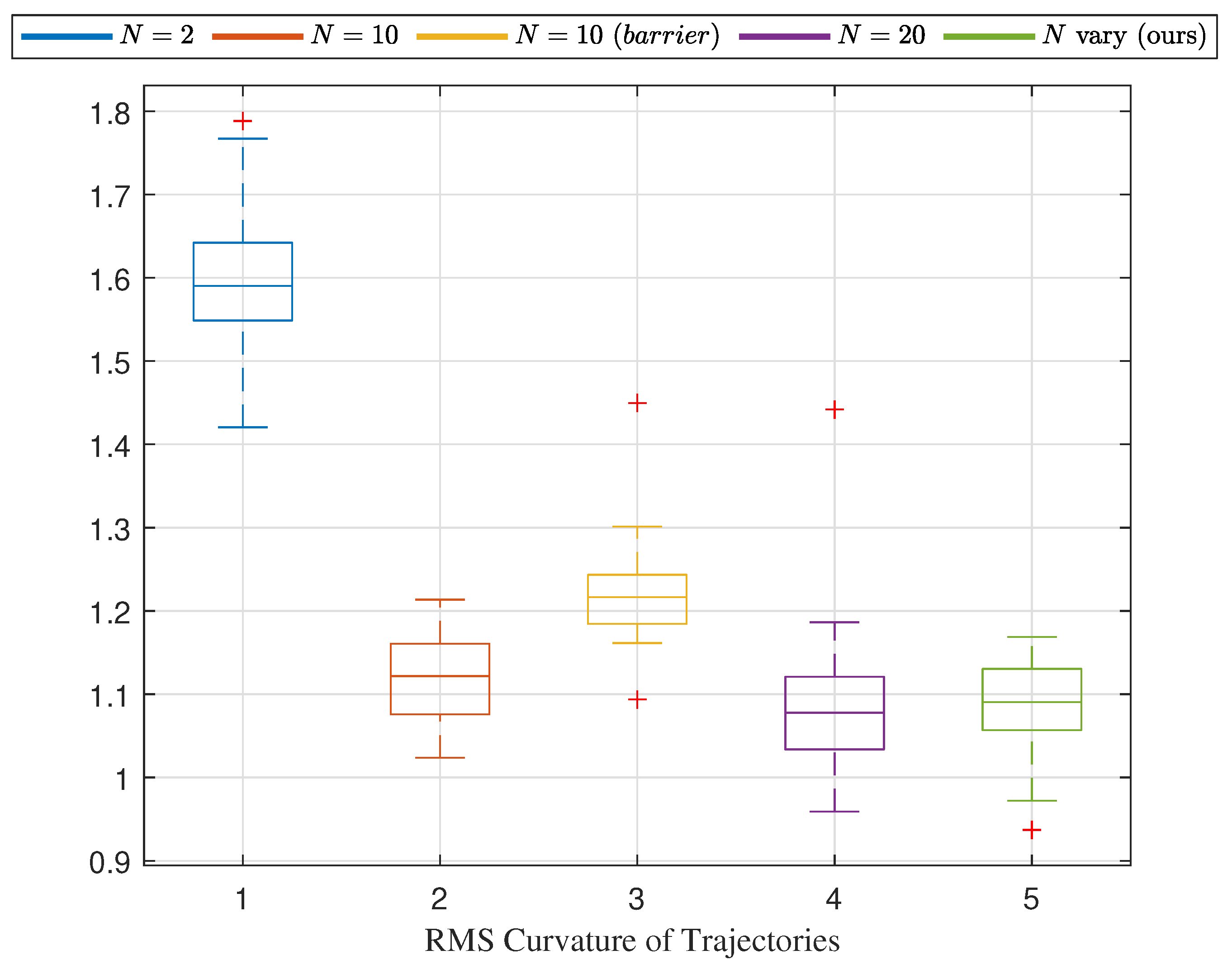
As shown in Figure 7, the trajectory created by our method, which has a variable prediction horizon, is much smoother than the case with a fixed prediction horizon of 2. Furthermore, the figure illustrates that the measure of trajectory smoothness for the CBF-based MPC ( N = 10 ( b a r r i e r ) ) is slightly worse than the same standard MPC without CBF ( N = 10 ) with the same horizon, partly due to the CBF-MPC’s aim of maintaining safe distance to the obstacles, which often means that it produces less smooth trajectories since the robot is more conservative in its adjustments to avoid collision.
In sum, we can see that our proposed method achieves a good balance between real-time performance and trajectory smoothness. In other words, dynamic adjustment of the prediction horizon of model predictive control indicates better performance in a control framework.

4.2. Real-World Scenario

The mobile robot and the computer comprise the hardware platform during experiments in the physical-World stage. The computer has the same settings as it did during the simulation stage. The robot is powered by an ESP32-WROOM-32U microcontroller, manufactured by Espressif Systems, based in Shanghai, China. This microcontroller has 520 KB of SRAM and 4 MB of flash memory and uses Wi-Fi to send and receive movement commands to/from the robot. The robot also has a connection to the computer for sending and receiving information about sensor data and for performing algorithm computations in the Model Predictive Control (MPC) for determining control actions that the robot will perform.
For the sake of reliability in localization and safety, the speed limit on the robot during experiments was set to 0.1 m/s. The reason for using the speed limit of 0.1 m/s in the experiment is due to the increased chances of amplification of position errors with increasing speed, which would affect how well the robot performs in control and how safe it is during experimentation. Hence, the experiments adopted a low-speed setting to ensure reliable localization and to ensure safe performance during experiment validation.
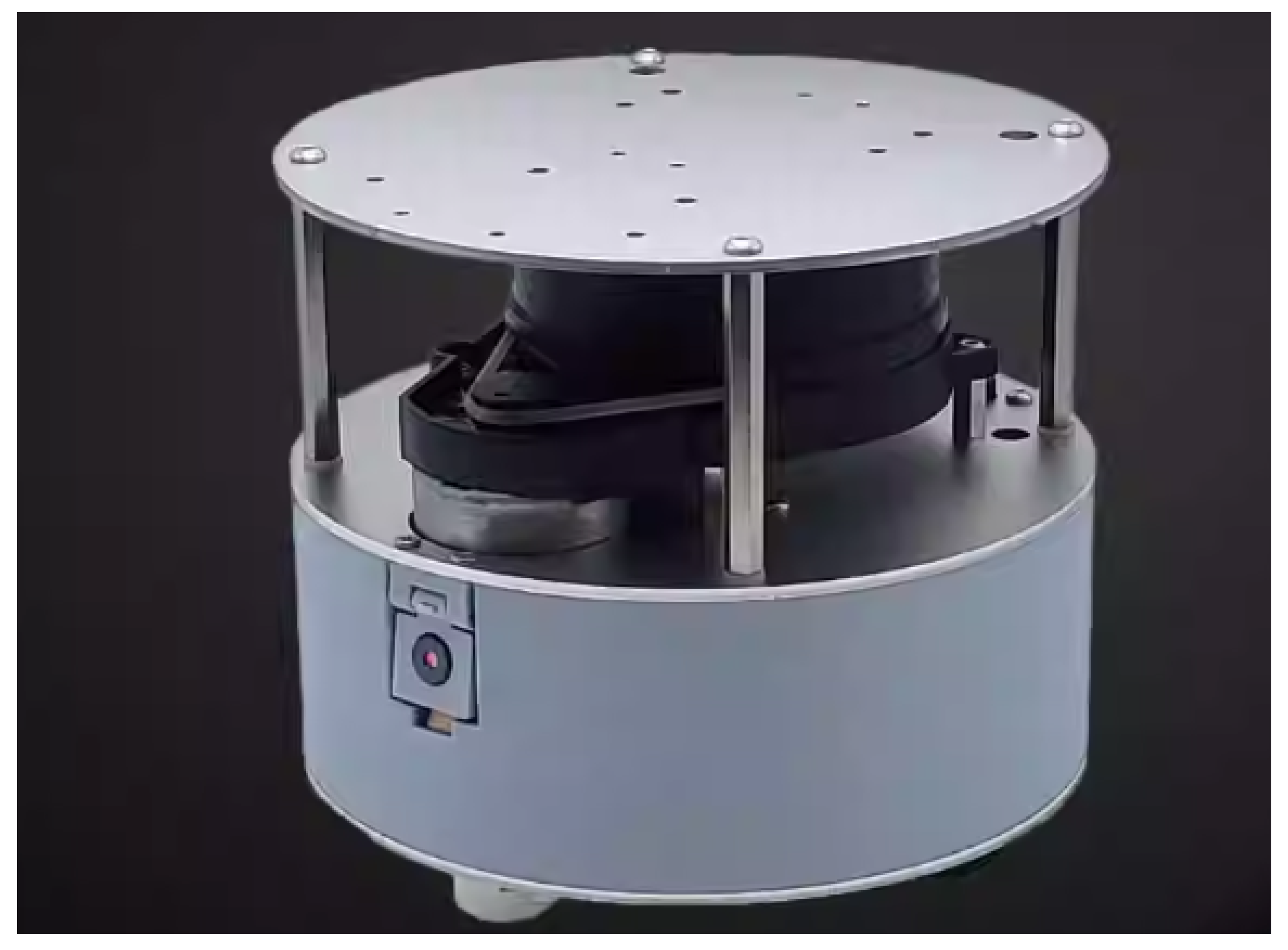
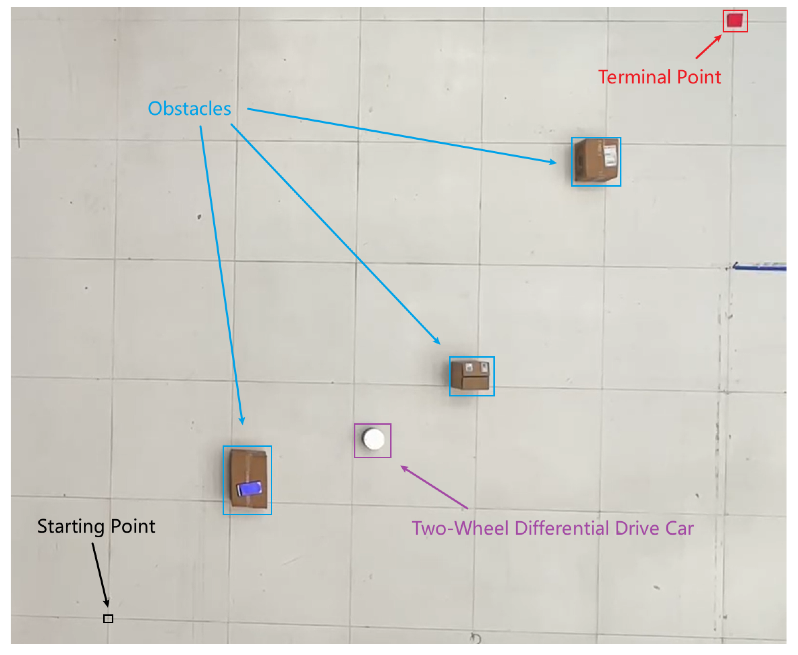
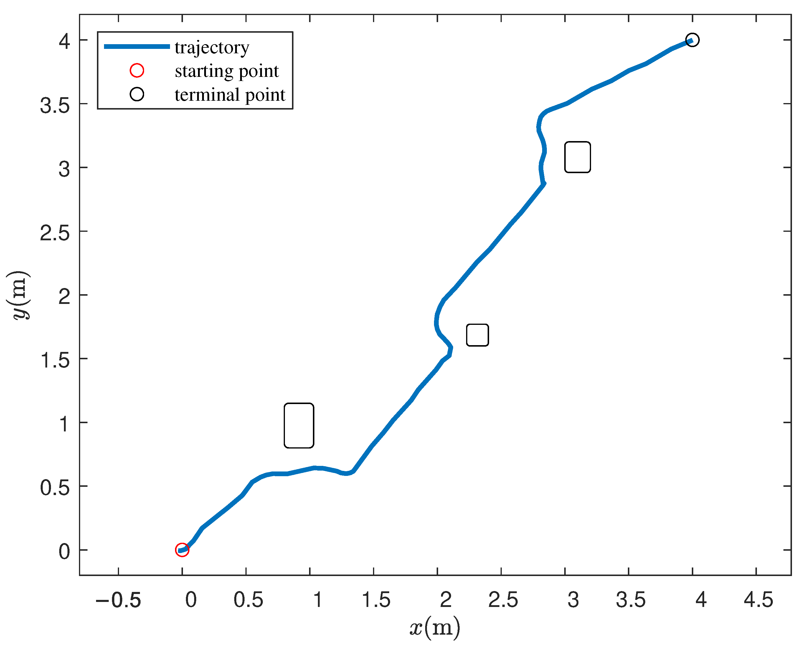
We use the Hawkbot robot, as shown in Figure 8. The robot has a diameter of 0.12 m, a chassis with two driving wheels and a supporting wheel, a LiDAR mounted in the center, and a high-definition camera at the front. The real-world scenario during the robot’s navigation is shown in Figure 9. The robot’s starting position is [0 m, 0 m], and the goal position is [4 m, 4 m]. The positions and sizes of the three obstacles have been changed. The three obstacles are confined within the x-y intervals [0.8 m, 1.03 m] × [0.8 m, 1.15 m], [2.23 m, 2.4 m] × [1.6 m, 1.77 m], and [3.0 m, 3.2 m] × [2.96 m, 3.2 m]. The maximum allowable velocity of the robot is set to 0.1 m/s, and the prediction cycle for solving the optimization problem is adjusted to 0.5 s. Other parameters remain consistent with the simulation scenario. Our robot’s localization is implemented using the commonly used Adaptive Monte Carlo Localization algorithm [45,46]. The obtained robot trajectory is shown in Figure 10.
During the navigation process, when the robot encounters an obstacle, it dynamically adjusts the prediction horizon based on the size of the obstacle ahead in real-time. This real-time adjustment helps to optimize the predicted trajectory, improving the robot’s ability to avoid obstacles. The robot’s trajectory can be seen in Figure 10. When the robot moves away from obstacles, it switches to a shorter prediction horizon to improve real-time performance. When encountering three different obstacles, the obstacle avoidance distance and prediction horizon are adjusted accordingly to achieve better navigation results.
The trajectory shown in Figure 10 might look a bit jagged. This is mainly because of some limitations in the real-world sensing system. During the experiment, the robot’s onboard localization wasn’t perfect, and the LiDAR sensor updated its obstacle distance measurements at a relatively low frequency. As a result, some of the recorded positions ended up being very similar or even repeated, causing small oscillations in the trajectory. These fluctuations are due to imperfections in the sensing and localization, not the navigation method itself.
The experiment revealed that the robot successfully applied the proposed prediction horizon method, allowing the robot to adapt to the different sizes and distances of the obstacles encountered during navigation. The predicted trajectory showed an ability to adapt smoothly to the different sizes and distances of obstacles.

5. Conclusions

To reach a balance between trajectory smoothness and real-time performance, this paper applies a new variable horizon model predictive control method for local navigation. The approach consists of two stages: optimal control parameter selection using an NSGA-II algorithm, and application to variable horizon control for the navigation of differential-drive robots. Using simulation, we show that the proposed algorithm greatly enhances real-time performance and helps maintain a smooth trajectory. In addition, real-world testing confirms the method’s effectiveness and practicality for actual operation.
Despite these advantages, the proposed approach has some limitations. For instance, its adaptability to highly dynamic or unpredictable obstacles is limited, since the current method relies on precomputed control parameters and may not fully respond to rapidly changing environments. Additionally, the method has been evaluated primarily in relatively structured scenarios; its performance in highly cluttered or uncertain environments remains to be tested. In future work, we plan to integrate reinforcement learning with MPC navigation to develop adaptive prediction horizon strategies, enabling the system to better handle diverse and dynamic scenarios, and further enhancing robustness and safety in more complex environments.

Author Contributions

Conceptualization, D.W., J.Z. and Z.F.; Methodology, D.W., G.W. and G.M.; Software, G.W., G.M. and W.L.; Validation, G.W., G.M. and D.W.; Formal analysis, G.W. and G.M.; Investigation, G.W., G.M. and K.B.; Resources, D.W. and Z.F.; Data curation, W.L.; Writing—original draft, G.W. and G.M.; Writing—review and editing, D.W., K.B., W.L. and Z.F.; Visualization, G.W. and G.M.; Supervision, D.W. and Z.F.; Project administration, D.W.; Funding acquisition, Z.F. and G.W.; All authors have read and agreed to the published version of the manuscript.

Funding

This research is funded by the National Natural Science Foundation of China (grant number 62472111), the Science and Technology Planning Project of Guangdong Province, China (grant numbers 2022A1515110566, 2023A1515011574, 2025A1515011338).

Institutional Review Board Statement

Not applicable.

Informed Consent Statement

Not applicable.

Data Availability Statement

The original contributions presented in this study are included in the article. Further inquiries can be directed to the corresponding author.

Conflicts of Interest

The authors declare no conflicts of interest.

References

  1. Hart, P.E.; Nilsson, N.J.; Raphael, B. A formal basis for the heuristic determination of minimum cost paths. IEEE Trans. Syst. Sci. Cybern. 1968, 4, 100–107. [Google Scholar] [CrossRef]
  2. Niu, J.; Zhang, L.; Zhang, T.; Guan, J.; Shi, S. Orchard Robot Navigation via an Improved RTAB-Map Algorithm. Appl. Sci. 2025, 15, 11673. [Google Scholar] [CrossRef]
  3. Stentz, A. The focussed d* algorithm for real-time replanning. In Proceedings of the International Joint Conference on Artificial Intelligence, Montreal, QC, Canada, 20–25 August 1995; Volume 95, pp. 1652–1659. [Google Scholar]
  4. Ambrożkiewicz, M.; Bonar, B.; Buratowski, T.; Małka, P. Advanced probabilistic roadmap path planning with adaptive sampling and smoothing. Electronics 2025, 14, 3804. [Google Scholar] [CrossRef]
  5. Wang, J.; Pang, T.; Zhang, W.; Liao, W.; Du, T. Research on Path Planning Based on Multi-Dimensional Optimized RRT Algorithm. World Electr. Veh. J. 2025, 16, 605. [Google Scholar] [CrossRef]
  6. Fox, D.; Burgard, W.; Thrun, S. The dynamic window approach to collision avoidance. IEEE Robot. Autom. Mag. 1997, 4, 23–33. [Google Scholar] [CrossRef]
  7. Borenstein, J.; Koren, Y. The vector field histogram-fast obstacle avoidance for mobile robots. IEEE Trans. Robot. Autom. 1991, 7, 278–288. [Google Scholar] [CrossRef]
  8. Tonko, J.; Ruiperez-Campillo, S.; Cabero-Vidal, G.; Rooney, C.; Ehnesh, M.; Millet-Roig, J.; Castells, P.; Lambiase, P. Vector Field Heterogeneity (VFH) as a novel quantitative marker of electrical disarray in Arrhythmogenic CardioMyopathy (ACM) with ventricular tachycardia. Eur. Heart J. 2024, 45, ehae666.654. [Google Scholar] [CrossRef]
  9. Khatib, O. Real-time obstacle avoidance for manipulators and mobile robots. Int. J. Robot. Res. 1986, 5, 90–98. [Google Scholar] [CrossRef]
  10. Hu, Y.; Zhou, W.; Liu, Y.; Zeng, M.; Ding, W.; Li, S.; Li, G.; Li, Z.; Knoll, A. Efficient online planning and robust optimal control for nonholonomic mobile robot in unstructured environments. IEEE Trans. Emerg. Top. Comput. Intell. 2024, 8, 3559–3575. [Google Scholar] [CrossRef]
  11. Ratliff, N.; Zucker, M.; Bagnell, J.A.; Srinivasa, S. CHOMP: Gradient optimization techniques for efficient motion planning. In Proceedings of the 2009 IEEE International Conference on Robotics and Automation, Kobe, Japan, 12–17 May 2009; IEEE: Piscataway, NJ, USA, 2009; pp. 489–494. [Google Scholar]
  12. Schulman, J.; Ho, J.; Lee, A.X.; Awwal, I.; Bradlow, H.; Abbeel, P. Finding locally optimal, collision-free trajectories with sequential convex optimization. In Proceedings of the Robotics: Science and Systems, Berlin, Germany, 24–28 June 2013; Volume 9, pp. 1–10. [Google Scholar]
  13. Benders, D.; Köhler, J.; Niesten, T.; Babuška, R.; Alonso-Mora, J.; Ferranti, L. Embedded hierarchical MPC for autonomous navigation. IEEE Trans. Robot. 2025, 41, 3556–3574. [Google Scholar] [CrossRef]
  14. Wang, Z.; Wang, S.; Xie, Y.; Xiong, T.; Wang, C. Autonomous Navigation of Mobile Robots: A Hierarchical Planning–Control Framework with Integrated DWA and MPC. Sensors 2025, 25, 2014. [Google Scholar] [CrossRef]
  15. Zeng, J.; Zhang, B.; Sreenath, K. Safety-critical model predictive control with discrete-time control barrier function. In Proceedings of the 2021 American Control Conference (ACC), New Orleans, LA, USA, 25–28 May 2021; IEEE: Piscataway, NJ, USA, 2021; pp. 3882–3889. [Google Scholar]
  16. Breeden, J.; Panagou, D. Predictive control barrier functions for online safety critical control. In Proceedings of the 2022 IEEE 61st Conference on Decision and Control (CDC), Cancun, Mexico, 6–9 December 2022; IEEE: Piscataway, NJ, USA, 2022; pp. 924–931. [Google Scholar]
  17. Bøhn, E.; Gros, S.; Moe, S.; Johansen, T.A. Reinforcement learning of the prediction horizon in model predictive control. IFAC-PapersOnLine 2021, 54, 314–320. [Google Scholar] [CrossRef]
  18. Quartullo, R.; Bianchini, G.; Garulli, A.; Giannitrapani, A. Robust variable-horizon MPC with adaptive terminal constraints. Automatica 2025, 179, 112465. [Google Scholar] [CrossRef]
  19. Chen, Z.; Lai, J.; Li, P.; Awad, O.I.; Zhu, Y. Prediction horizon-varying model predictive control (MPC) for autonomous vehicle control. Electronics 2024, 13, 1442. [Google Scholar] [CrossRef]
  20. Seder, M.; Klančar, G. Convergent wheeled robot navigation based on an interpolated potential function and gradient. Robot. Auton. Syst. 2024, 177, 104712. [Google Scholar] [CrossRef]
  21. Ding, Y.; Wang, L.; Li, Y.; Li, D. Model predictive control and its application in agriculture: A review. Comput. Electron. Agric. 2018, 151, 104–117. [Google Scholar] [CrossRef]
  22. Wang, L.; Wang, G.; Li, Y.; Li, P.; Ji, Y.; Wang, C.; Shen, Y. Real-time whole-body collision avoidance and path following of a snake robot through MPC-based optimization strategies. In Proceedings of the 2023 IEEE/RSJ International Conference on Intelligent Robots and Systems (IROS), Detroit, MI, USA, 1–5 October 2023; IEEE: Piscataway, NJ, USA, 2023; pp. 2362–2367. [Google Scholar]
  23. Rawlings, J.B.; Mayne, D.Q.; Diehl, M. Model Predictive Control: Theory, Computation, and Design; Nob Hill Publishing: Madison, WI, USA, 2017; Volume 2. [Google Scholar]
  24. Brito, B.; Floor, B.; Ferranti, L.; Alonso-Mora, J. Model predictive contouring control for collision avoidance in unstructured dynamic environments. IEEE Robot. Autom. Lett. 2019, 4, 4459–4466. [Google Scholar] [CrossRef]
  25. Gao, F.; Wu, W.; Lin, Y.; Shen, S. Online safe trajectory generation for quadrotors using fast marching method and bernstein basis polynomial. In Proceedings of the 2018 IEEE International Conference on Robotics and Automation (ICRA), Brisbane, Australia, 21–25 May 2018; IEEE: Piscataway, NJ, USA, 2018; pp. 344–351. [Google Scholar]
  26. Gao, F.; Lin, Y.; Shen, S. Gradient-based online safe trajectory generation for quadrotor flight in complex environments. In Proceedings of the 2017 IEEE/RSJ International Conference on Intelligent Robots and Systems (IROS), Vancouver, BC, Canada, 24–28 September 2017; IEEE: Piscataway, NJ, USA, 2017; pp. 3681–3688. [Google Scholar]
  27. Lopez, B.T.; How, J.P. Aggressive 3-D collision avoidance for high-speed navigation. In Proceedings of the 2017 IEEE International Conference on Robotics and Automation (ICRA), Singapore, 29 May–3 June 2017; pp. 5759–5765. [Google Scholar]
  28. Wang, S.; Wang, Y.; Miao, Z.; Wang, X.; He, W. Dual model predictive control of multiple quadrotors with formation maintenance and collision avoidance. IEEE Trans. Ind. Electron. 2024, 71, 16037–16046. [Google Scholar] [CrossRef]
  29. Mayne, D. A second-order gradient method for determining optimal trajectories of non-linear discrete-time systems. Int. J. Control 1966, 3, 85–95. [Google Scholar] [CrossRef]
  30. Liao, L.Z.; Shoemaker, C.A. Advantages of Differential Dynamic Programming over Newton’s Method for Discrete-Time Optimal Control Problems; Technical Report; Cornell University: Ithaca, NY, USA, 1992. [Google Scholar]
  31. Bock, H.G.; Plitt, K.J. A multiple shooting algorithm for direct solution of optimal control problems. IFAC Proc. Vol. 1984, 17, 1603–1608. [Google Scholar] [CrossRef]
  32. Diehl, M.; Bock, H.G.; Diedam, H.; Wieber, P.B. Fast direct multiple shooting algorithms for optimal robot control. In Fast Motions in Biomechanics and Robotics: Optimization and Feedback Control; Springer: Berlin/Heidelberg, Germany, 2006; pp. 65–93. [Google Scholar]
  33. Li, H.; Yu, W.; Zhang, T.; Wensing, P.M. A unified perspective on multiple shooting in differential dynamic programming. In Proceedings of the 2023 IEEE/RSJ International Conference on Intelligent Robots and Systems (IROS), Detroit, MI, USA, 1–5 October 2023; IEEE: Piscataway, NJ, USA, 2023; pp. 9978–9985. [Google Scholar]
  34. Marcucci, T.; Tedrake, R. Warm start of mixed-integer programs for model predictive control of hybrid systems. IEEE Trans. Autom. Control 2020, 66, 2433–2448. [Google Scholar] [CrossRef]
  35. Wang, Z.; Pei, Y.; Li, J. A survey on search strategy of evolutionary multi-objective optimization algorithms. Appl. Sci. 2023, 13, 4643. [Google Scholar] [CrossRef]
  36. Yi, J.; Zhang, C.; Chen, S.; Dai, Q.; Yu, H.; Yang, G.; Yu, L. Multi-objective optimal trajectory planning for woodworking manipulator and worktable based on the INSGA-II algorithm. Appl. Sci. 2024, 15, 310. [Google Scholar] [CrossRef]
  37. Zhang, Q.; Li, H. MOEA/D: A multiobjective evolutionary algorithm based on decomposition. IEEE Trans. Evol. Comput. 2007, 11, 712–731. [Google Scholar] [CrossRef]
  38. Emmerich, M.; Beume, N.; Naujoks, B. An EMO algorithm using the hypervolume measure as selection criterion. In Proceedings of the International Conference on Evolutionary Multi-Criterion Optimization, Guanajuato, Mexico, 9–11 March 2005; Springer: Berlin/Heidelberg, Germany, 2005; pp. 62–76. [Google Scholar]
  39. Deb, K.; Pratap, A.; Agarwal, S.; Meyarivan, T. A fast and elitist multiobjective genetic algorithm: NSGA-II. IEEE Trans. Evol. Comput. 2002, 6, 182–197. [Google Scholar] [CrossRef]
  40. Qazani, M.R.C.; Karkoub, M.; Asadi, H.; Lim, C.P.; Liew, A.W.C.; Nahavandi, S. Multi-objective NSGA-II for weight tuning of a nonlinear model predictive controller in autonomous vehicles. In Proceedings of the 2022 IEEE International Conference on Systems, Man, and Cybernetics (SMC), Prague, Czech Republic, 9–12 October 2022; IEEE: Piscataway, NJ, USA, 2022; pp. 2820–2826. [Google Scholar]
  41. Arshad, M.H.; Abido, M.A.; Salem, A.; Elsayed, A.H. Weighting factors optimization of model predictive torque control of induction motor using NSGA-II with TOPSIS decision making. IEEE Access 2019, 7, 177595–177606. [Google Scholar] [CrossRef]
  42. Andersson, J.A.E.; Gillis, J.; Horn, G.; Rawlings, J.B.; Diehl, M. CasADi—A software framework for nonlinear optimization and optimal control. Math. Program. Comput. 2019, 11, 1–36. [Google Scholar] [CrossRef]
  43. Wächter, A.; Biegler, L.T. On the implementation of an interior-point filter line-search algorithm for large-scale nonlinear programming. Math. Program. 2006, 106, 25–57. [Google Scholar] [CrossRef]
  44. Jian, Z.; Yan, Z.; Lei, X.; Lu, Z.; Lan, B.; Wang, X.; Liang, B. Dynamic Control Barrier Function-based Model Predictive Control to Safety-Critical Obstacle-Avoidance of Mobile Robot. In Proceedings of the 2023 IEEE International Conference on Robotics and Automation (ICRA), London, UK, 29 May–2 June 2023; pp. 3679–3685. [Google Scholar]
  45. Thrun, S.; Burgard, W.; Fox, D. Probabilistic Robotics; The MIT Press: Cambridge, MA, USA, 2005. [Google Scholar]
  46. Zuo, C.; Xie, D.; Wu, L.; Tang, X.; Zhang, H. An Improved Adaptive Monte Carlo Localization Algorithm Integrated with a Virtual Motion Model. Sensors 2025, 25, 2471. [Google Scholar] [CrossRef]
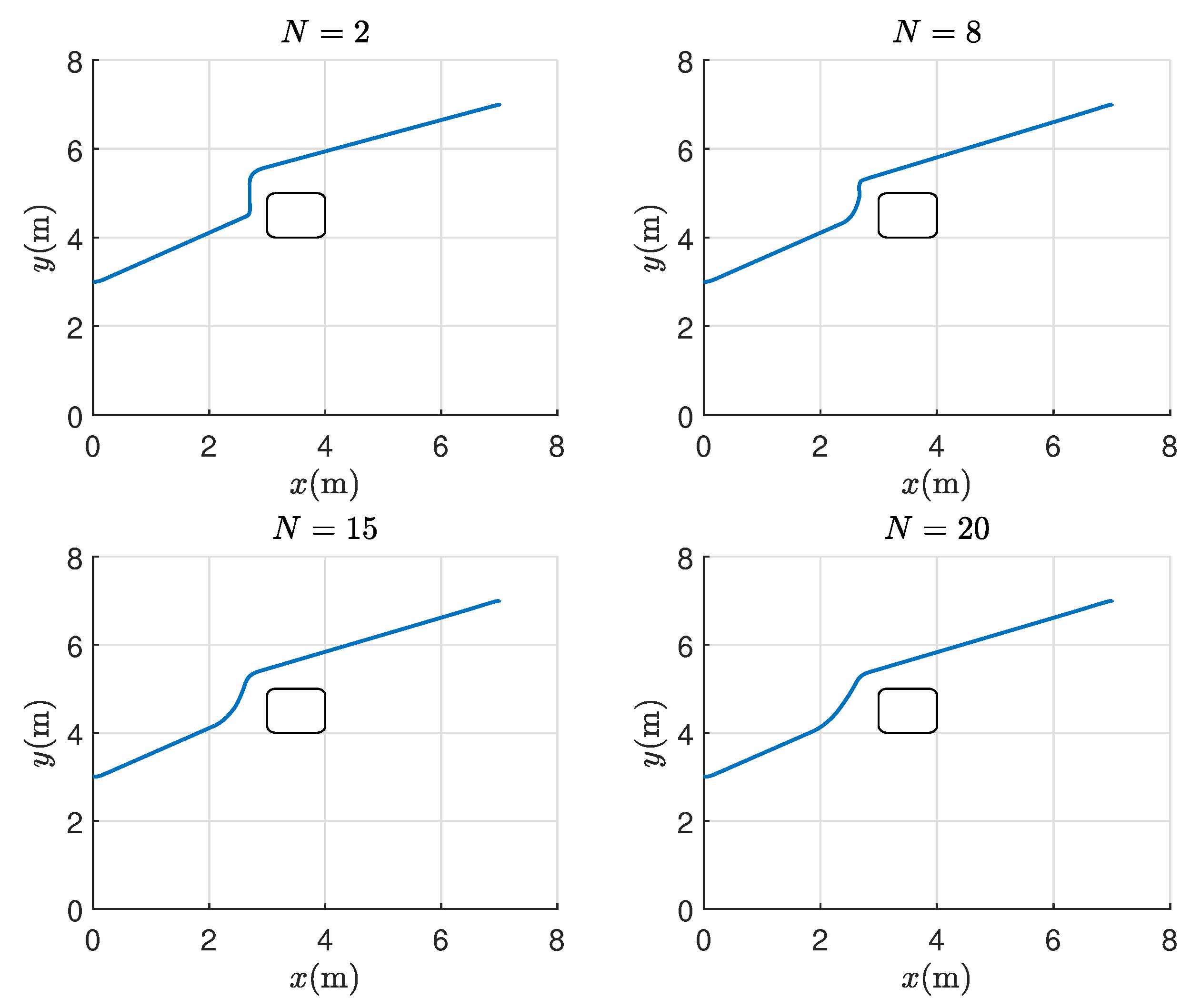
Figure 1. The navigation trajectory plots for different prediction horizons implemented using MPC. Here, N represents the prediction horizon, corresponding to values of 2, 8, 15, and 20. The start position is [0 m, 3 m], and the goal position is [7 m, 7 m]. The blue lines represent the navigation trajectory, and the black boxes indicate obstacles.
Electronics 15 00603 g001
Figure 2. Overview diagram of variable horizon model predictive control based on NSGA-II. The different blue boxes represent different modules, and the arrows between modules indicate the transfer of variables. The large yellow box denotes online computation.
Electronics 15 00603 g002
Figure 3. The Pareto front generated by the NSGA-II algorithm. Blue points represent the non-dominated Pareto solutions of rank 1, while orange points represent those of rank 2. The x-axis is related to real-time performance, and the y-axis is related to safety. The optimization objectives are all minimized. The black box represents the selected optimal solution.
Electronics 15 00603 g003
Figure 4. Comparison of navigation trajectories between variable prediction horizon and fixed prediction horizon. N represents the prediction horizon. The starting point is [1 m, 1 m], and the terminal point is [7 m, 7 m]. The N = 10 ( b a r r i e r ) label indicates that the CBF constraint method was used. The black square, rectangle, and circle represent obstacles.
Electronics 15 00603 g004
Figure 5. A plot showing the variation of the prediction horizon over time during navigation.
Electronics 15 00603 g005
Figure 6. Comparison of real-time performance between variable and fixed prediction horizons. Num of Opti and Total Time represent the total number of optimizations and total time during navigation, respectively. The time unit is seconds. The N = 10 ( b a r r i e r ) label indicates that the CBF constraint method was used. The red “+” symbols represent outliers, which are data points that differ significantly from the rest of the data.
Electronics 15 00603 g006
Figure 7. Comparison of trajectory smoothness metrics between variable and fixed prediction horizons. The red “+” symbols represent outliers, which are data points that differ significantly from the rest of the data.
Electronics 15 00603 g007
Figure 8. The two-wheels car used in real-world experiment.
Electronics 15 00603 g008
Figure 9. A top-down view of the real-world scenario, including obstacles, the car, the starting point, and the navigation terminal point.
Electronics 15 00603 g009
Figure 10. The robot’s trajectory in the real-world experiment. The starting point is [0 m, 0 m], and the terminal point is [4 m, 4 m]. The squares and rectangles represent obstacles in the environment.
Electronics 15 00603 g010
Table 1. The average values from the twenty experiments.
Num of OptiTotal Time (s)Num of Opti/Total Time
N = 2 3126.519.654159
N = 10 2272.319.173118.48
N = 10 ( b a r r i e r )2188.919.318113.16
N = 20 1664.218.96387.694
N vary2663.918.783141.67
Disclaimer/Publisher’s Note: The statements, opinions and data contained in all publications are solely those of the individual author(s) and contributor(s) and not of MDPI and/or the editor(s). MDPI and/or the editor(s) disclaim responsibility for any injury to people or property resulting from any ideas, methods, instructions or products referred to in the content.