A Methodology for Microcrack Detection in Plate Heat Exchanger Sheets Using Adaptive Templates and Features Value Analysis

Abstract

Aiming at the detection challenges caused by the diverse morphology of microcracks in plate heat exchanger sheets, this paper proposes a detection framework that integrates parameter-driven adaptive template generation, binary scale optimization, and feature value threshold segmentation using convolutional networks. First, based on the grayscale characteristics of microcracks, an adaptive template generation model driven by key parameters (width, height, and endpoint grayscale difference) is constructed, obtaining a unique solution by solving the boundary conditions of physical features. Second, to overcome the challenge of microcrack width continuity, a binary scale optimization strategy based on the critical decay ratio k* of the correlation coefficient is designed, enabling the coverage of continuous-width defects with a finite set of templates. Finally, enhanced features are fed into a convolutional network. Utilizing the bimodal characteristic of the feature value distribution, the region corresponding to the extreme values in the top 0.3% before the foreground peak is located using 3σ extreme value statistics, achieving adaptive segmentation to identify defect regions. Evaluation on the self-built microcrack dataset SUT-B1 yielded results of 83.59% recall, 80.55% precision, and an F1 score of 81.98%. This method outperforms small object detection networks, demonstrating its advantage in morphological adaptability for small-sized objects. It also surpasses receptive field optimization modules, proving the necessity of structural optimization. The proposed method demonstrates practicality and scalability in the field of industrial inspection.

1. Introduction

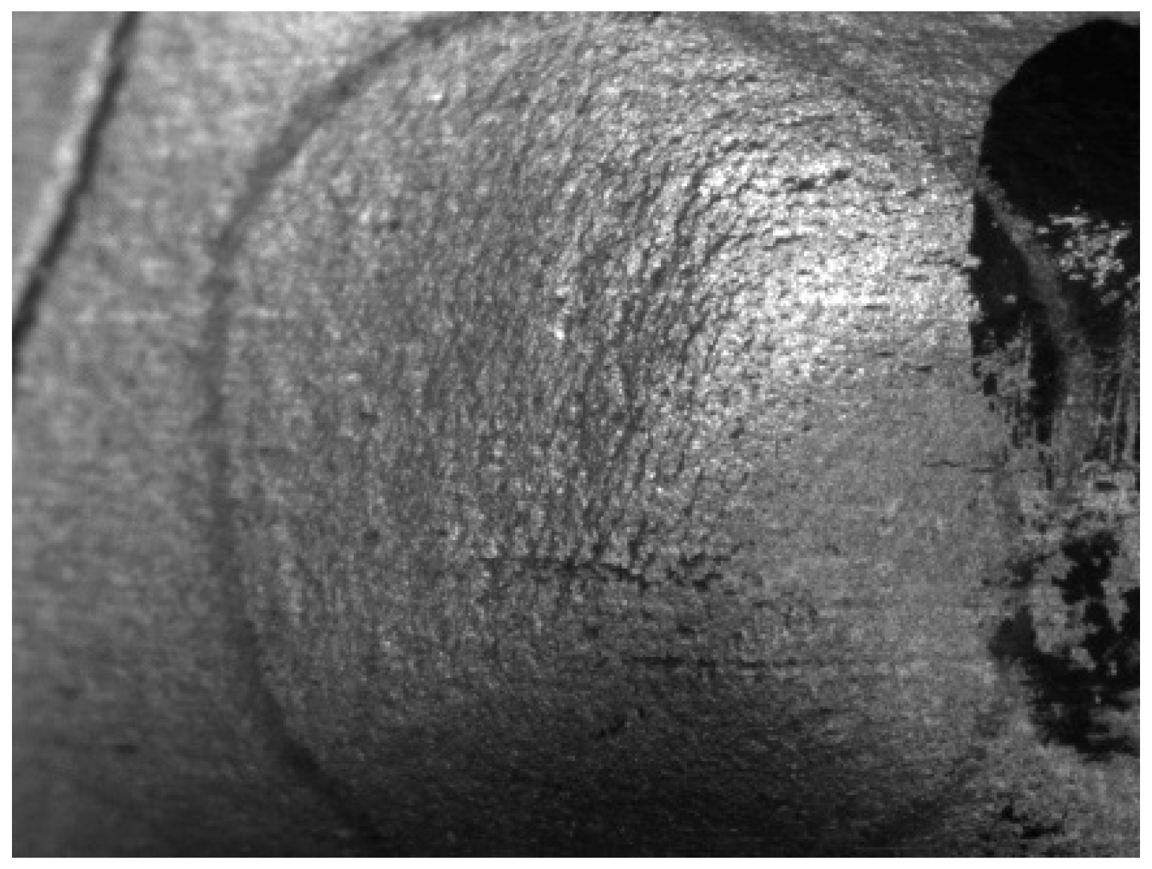
Removable plate heat exchangers (PHEs) are devices that utilize stacked corrugated metal sheets to facilitate heat transfer [1]. During the pressing process in sheet production, stamping techniques may induce the formation of minute linear defects on the sheet surfaces, known as microcracks. The application of localized stress can cause these microcracks to propagate and aggregate, forming clusters exhibiting linear grayscale characteristics. This study collectively defines such clusters as microcrack defects. These defects pose a risk of cracking under internal pressure during equipment operation, particularly after water injection. According to the National Standard of the People’s Republic of China GB/T232-1988, “Metallic Materials—Bend Test Methods” [2], microcracks appearing on the metal substrate of the outer surface of a bent specimen are classified as microcracks if their length does not exceed 2 mm or their width does not exceed 0.2 mm. It should be noted that this quantitative definition for microcrack defects is explicitly recorded only in GB/T232-1988 and is omitted in the latest version, GB/T232-2024 [3]. Furthermore, the Energy Industry Standard of the People’s Republic of China NB/T47004.1-2017, “Plate Heat Exchangers—Part 1: Removable Plate Heat Exchangers,” [4] specifies that the core requirement for microcrack detection is the determination of defect existence, without the necessity for precise measurement of length parameters.

Currently, defect detection for plate heat exchanger sheets in industrial production primarily relies on manual random sampling and penetrant testing leak testing methods. Manual visual inspection suffers from inherent drawbacks such as low efficiency, high subjectivity, and susceptibility to fatigue, making it unsuitable for large-scale industrial requirements. Automated visual inspection technologies, particularly methods based on image processing and machine learning, have become a research focus.

Traditional methods depend on manually designed feature enhancement templates. Among these, microcrack defects exhibiting linear grayscale characteristics can be detected using Gaussian template matching [5] or edge detection template matching based on gradients or curvature, such as the Canny operator [6], Gabor operator [7], and Otsu thresholding [8]. While effective under conditions characterized by a single grayscale feature, these traditional methods struggle to handle the morphologically diverse nature of microcrack defects, necessitating the consideration of feature enhancement rules.

Convolutional neural networks (CNNs) have been widely applied in the field of object detection [9,10,11,12]. Existing methods primarily fall into three categories: Single-stage regression-based algorithms, such as Hao et al. [13], who addressed the scarcity of strip steel surface defect samples by proposing a ResNet34 classification model fused with a Generative Adversarial Network and attention mechanism, enhancing samples through noise generation; Feng et al. [14] combined ResNet50 with a convolutional attention module to improve classification accuracy for strip steel defects; Two-stage region proposal-based algorithms, such as Nagy et al. [15], who employed EfficientNet with an Extreme Learning Machine for steel defect classification, and Zhang et al. [16], whose Mask R-CNN based on EfficientNet demonstrated excellent performance for large object detection but suffered from small object detail loss due to low-resolution feature extraction; End-to-end Transformer-based algorithms, such as Anvar et al. [17], who directly utilized ShuffleNet for classifying the NEU dataset, and Xing et al. [18], who fused ShuffleNet-V2 with Vision Transformers (ViT) to compensate for the lack of convolutional prior knowledge, although the global attention mechanism still struggles to capture subtle features. However, the common challenge persists: On one hand, information pertaining to microcracks—characterized by their small size and low contrast—is prone to being obscured within complex backgrounds, necessitating more refined feature enhancement strategies. On the other hand, detection models typically output direct probability scores, overlooking the rich spatial and similarity information inherent in the feature maps themselves, making it difficult to distinguish false positives.

Receptive field optimization strategies within convolutional networks can also achieve feature enhancement for specific targets. For instance, Chen et al. [19] proposed the atrous spatial pyramid pooling module (ASPP), which employs parallel dilated convolutions to construct a spatial pyramid for capturing multi-scale context. Liu et al. [20] designed the receptive field block module (RFB), simulating the mechanism of the human visual receptive field to enhance feature diversity through multi-branch dilated convolutions. Additionally, Chen et al. [21] proposed dynamic region-aware convolution (DRConv), which utilizes dynamic region-aware convolution to adaptively learn kernel weights based on spatial location. While effective in principle, these methods still suffer from introducing background interference during feature learning and exhibit a tendency to overfit in industrial small sample scenarios.

To address the aforementioned challenges, this paper proposes a novel detection framework integrating parameter-adaptive template generation, binary scale optimization, and feature value threshold segmentation within a convolutional neural network. Firstly, the framework dynamically constructs a model based on the morphological parameters of linear objects, enabling morphological parameter-driven adaptive template generation to precisely match object features. Secondly, a binary scale optimization strategy, leveraging the decay characteristics of the template correlation coefficient, is introduced. By determining the critical ratio defining the applicable range of a template, this strategy achieves effective coverage of a continuous width using a finite number of templates. Finally, the enhanced features are fed into the convolutional neural network. Utilizing the bimodal distribution characteristics of the feature values and the 3σ extreme value statistical principle, a dynamic threshold segmentation model is constructed to detect the defective regions.

The remainder of this paper is organized as follows: Section 2 provides relevant background information and characteristics of microcracks. Section 3 details the proposed methodology. Section 4 describes the experimental datasets and evaluation metrics and presents and analyzes the experimental results. Section 5 provides an in-depth discussion of the results. Finally, Section 6 concludes the study.

2. Microcrack Defect Features

As a defect type in the plates of plate heat exchangers, the morphological characteristics of microcracks directly determine the effectiveness of detection methods. Research indicates that the formation mechanism of microcrack defects in these plates involves factors such as material stress distribution, fatigue loads, and manufacturing processes. Under their combined influence, microcracks often appear in clusters rather than as isolated entities. Figure 1 shows the high-resolution imaging, revealing that they manifest as spatially discrete local segments, each exhibiting a linear grayscale distribution with consistent directional alignment.

Analysis of quantitative data from the Shenyang University of Technology Benchmark Database (SUT-B1) reveals that the morphological characteristics of microcrack defects can be categorized into three key dimensions: first, they exhibit multi-scale characteristics in width, where pixel-level measurements show variations in crack width, rendering single-size templates inadequate for full-scale coverage. Second, the grayscale distribution approximates a Gaussian profile, with the central grayscale extremum exhibiting a non-linear decay towards both sides. Finally, a distinct asymmetry in the endpoints of the grayscale distribution is observed. Figure 2 illustrates these morphological variations: in the local regions of three defects on the left, embedded white lines indicate the positions of cross-sectional profiles, while the right side displays the corresponding grayscale distribution curves. It can be observed that there are inconsistencies in width and height between different defects, while individual cross-sections demonstrate the characteristic asymmetry in endpoint height and profile shape.

3. Proposed Method

This chapter systematically elaborates on the proposed method. First, building upon the analysis of microcrack morphological characteristics, a common linear feature model with an approximately Gaussian distribution is established, providing a theoretical foundation for the subsequent approach. Second, a parameterized adaptive template generation mechanism is designed. This mechanism dynamically constructs optimal convolution kernels based on key morphological parameters (width, height, and endpoint grayscale difference) of linear objects. Third, to address the challenge posed by the continuous variation in the width of linear objects, a binary scale optimization strategy based on the decay characteristics of the correlation coefficient between templates is proposed. This strategy aims to effectively cover the entire continuous width range using a finite number of templates, thereby enhancing the specificity of feature extraction. Finally, the enhanced features are input into a convolutional neural network structure. Leveraging the bimodal distribution characteristics within the feature histogram space and the 3σ extreme value statistical principle, a dynamic threshold segmentation model is constructed to achieve object region identification. The specific design and implementation details of each component will be elaborated in the following subsections.

3.1. Defect Feature Analysis

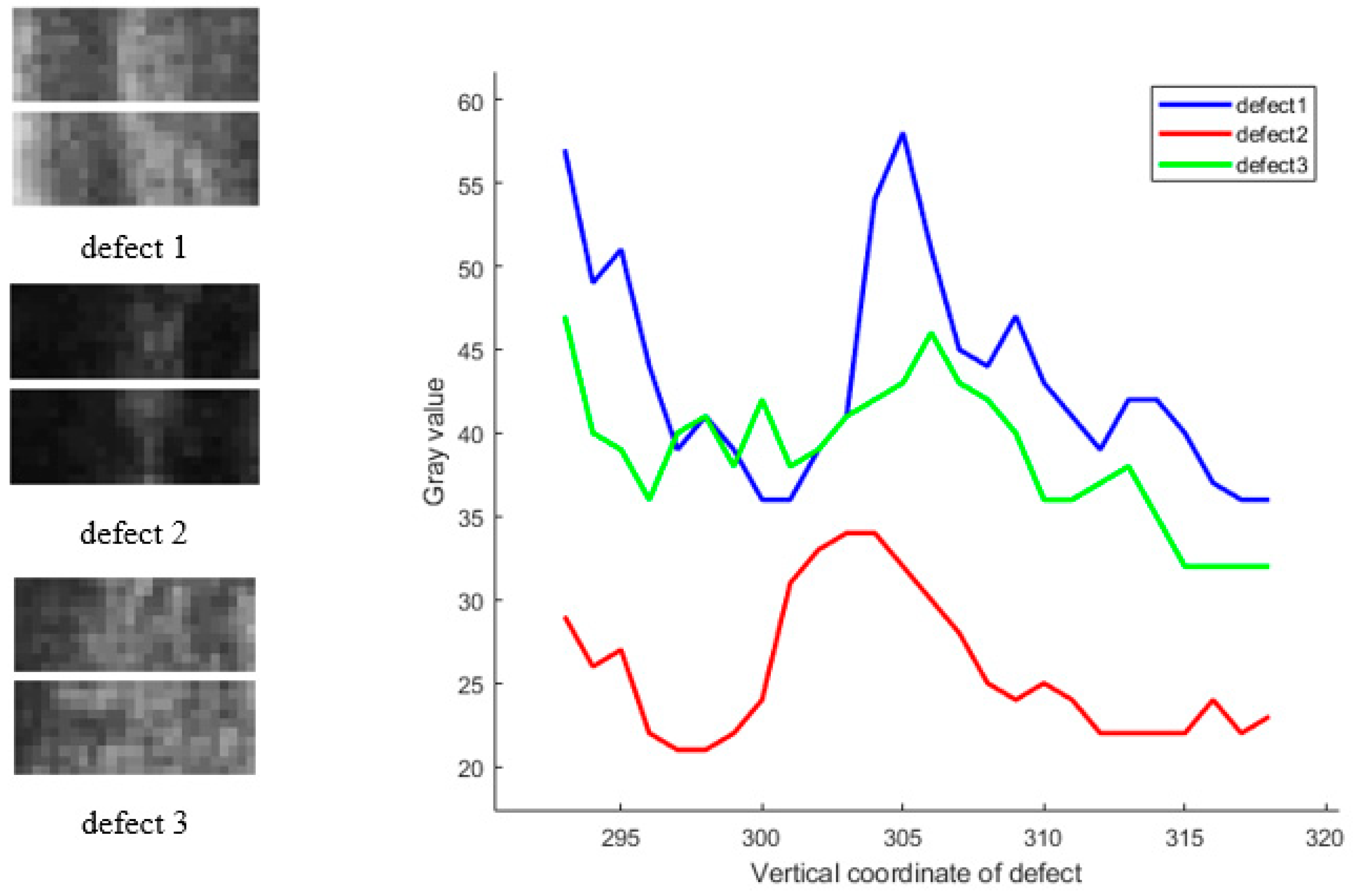
Following an in-depth analysis of the morphological characteristics of microcrack defects, they can be characterized by an approximately normal distribution profile: the central region of the microcrack exhibits a peak intensity, which gradually decreases towards both sides as the distance from the center increases, forming a declining trend. This decline is typically asymmetric, resulting in differences in the endpoint grayscale values. Although not strictly conforming to a normal distribution, this simplified mathematical model provides an effective framework for the morphological analysis of microcracks and extends to the broader domain of linear defects. Figure 3 sequentially illustrates the morphological features exhibiting variations in width, height, and endpoint grayscale differences.

3.2. Adaptive Template Design

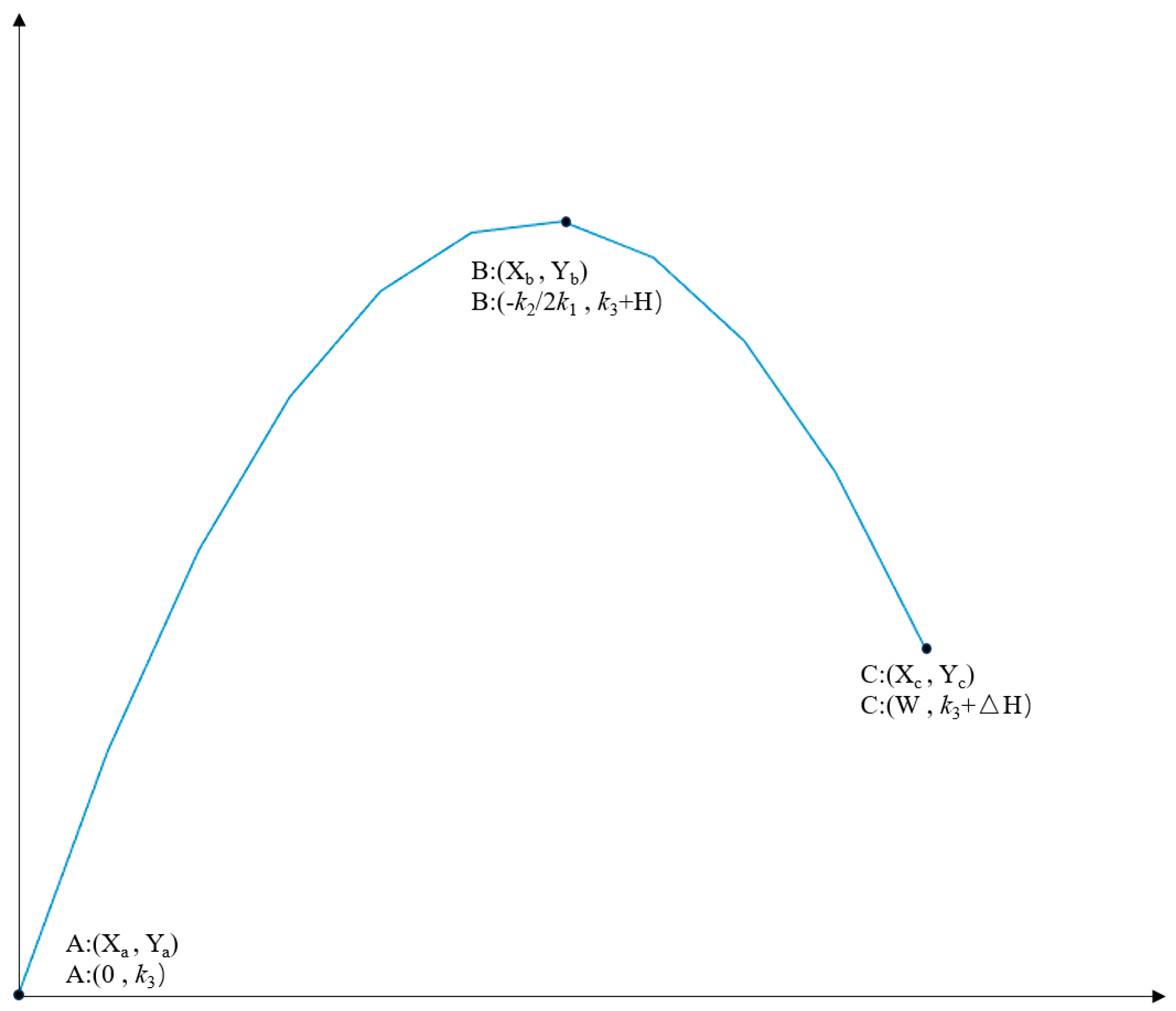
Traditional fixed-shape templates struggle to effectively match such morphologically variable objects, leading to degraded detection performance. Consequently, a template capable of adaptive generation based on the specific object’s morphological parameters is required. Let the defect’s starting point coordinates be denoted as (X_a, Y_a), the grayscale maximum point coordinates as (X_b, Y_b), and the endpoint coordinates as (X_c, Y_c). The required linear feature parameters can be parametrically expressed as follows: the actual width of the line, W: |X_c − X_a| = W; the height difference between the endpoints, ΔH: |Y_c − Y_a| = ΔH; and the actual height of the line, H: max{|Y_b − Y_c|, |Y_b − Y_a|}. These three parameters correspond to three boundary conditions, thereby uniquely determining a mathematical expression containing up to three coefficient variables. Given that the number of parameters is three, the expression can be modeled as a quadratic function, incorporating a quadratic coefficient k₁, a linear coefficient k₂, and a constant term k₃, as shown in Equation (1).

$$\mathrm{F}(x)=k_1\times x^2+k_2\times x+k_3$$

(1)

Taking the case where the defect’s minimum grayscale point is located at the starting point as an example, substituting into Equation (1) yields the following coordinate expressions: the starting point at (0, k₃), the grayscale maximum point at (X_b, k₃ + H), and the endpoint at (W, k₃ + ΔH). The three specific boundary conditions are:

1.

The template function possesses an integral value of zero over its domain, mathematically formalized by the boundary conditions in Equation (2). This fundamental property is physically meaningful: it ensures that the convolution response approaches zero against a uniform image background, thereby suppressing interference from homogeneous regions. Consequently, the template generates significant responses only when convolved with local structures morphologically matching its design. However, in practical industrial scenarios where backgrounds exhibit textures, noise, or gradient illumination, the zero-integral assumption may not hold perfectly, leading to non-zero responses in non-defective areas. The feature distribution analysis and segmentation techniques in the subsequent design phase are utilized to distinguish between noise and genuine defect responses.

$${\displaystyle {\int }_0^{\mathrm{W}}\mathrm{F}(x)\mathrm{dx}=0}\to {\displaystyle \frac{k_1}{3}}\times {\mathrm{W}}^3+{\displaystyle \frac{k_2}{2}}\times {\mathrm{W}}^2+k_3\mathrm{W}=0$$

(2)

2.

The function exhibits a derivative of zero at the grayscale maximum point, indicating a local extremum. Furthermore, the difference between the maximum and minimum grayscale values equals the actual height H. These critical constraints governing the template’s extremum properties are formally defined by the boundary conditions in Equation (3).

$$\left\{\begin{array}{c}{F}^{\prime }(X_b)=0\\ F(X_b)-F(0)=\mathrm{H}\end{array}\to \left\{\begin{array}{c}2k_1\times X_b+k_2=0\to X_b=-k_2/2k_1\\ k_1\times {(-k_2/2k_1)}^2+k_2\times (-k_2/2k_1)=\mathrm{H}\end{array}\right.\right.$$

(3)

3.

The domain width of the function is constrained to match the actual width W. Additionally, the difference in function values between the start and end points must equal the grayscale difference ΔH measured at these endpoints. These functional constraints are rigorously enforced by the boundary conditions specified in Equation (4).

$$F(\mathrm{W})-F(0)=\mathrm{\Delta }\mathrm{H}\to k_1\times {\mathrm{W}}^2+k_2\times \mathrm{W}=\mathrm{\Delta }\mathrm{H}$$

(4)

Through Equations (2)–(4), two sets of quadratic function coefficients (k₁, k₂, and k₃) are derived. By introducing the supplementary constraint that the position of the maximum must lie within the domain—formalized in Equation (5)—the invalid solutions are discarded, yielding a unique valid closed-form solution for the parameters. The resulting continuous filter function is given in Equation (6), with its conceptual representation illustrated in Figure 4.

$$0<{\mathrm{X}}_{\mathrm{b}}<\mathrm{W}({\mathrm{X}}_{\mathrm{b}}=-k_2/2k_1)$$

(5)

$$\left\{\begin{array}{c}\begin{array}{c}\begin{array}{l}{k}_1=-{\displaystyle \frac{(2\mathrm{H}-\mathrm{\Delta }\mathrm{H})-2\sqrt{{\mathrm{H}}^2-\mathrm{H}\mathrm{\Delta }\mathrm{H}}}{{\mathrm{W}}^2}}\\ k_2={\displaystyle \frac{2(\mathrm{H}+\sqrt{{\mathrm{H}}^2-\mathrm{H}\mathrm{\Delta }\mathrm{H}})}{\mathrm{W}}}\\ k_3={\displaystyle \frac{-\sqrt{{\mathrm{H}}^2-\mathrm{H}\mathrm{\Delta }\mathrm{H}}-\mathrm{H}-\mathrm{\Delta }\mathrm{H}}{3}}\end{array}\end{array}\\ \mathrm{F}(x)=-{\displaystyle \frac{(2\mathrm{H}-\mathrm{\Delta }\mathrm{H})-2\sqrt{{\mathrm{H}}^2-\mathrm{H}\mathrm{\Delta }\mathrm{H}}}{{\mathrm{W}}^2}}\times {\mathrm{x}}^2+{\displaystyle \frac{2(\mathrm{H}+\sqrt{{\mathrm{H}}^2-\mathrm{H}\mathrm{\Delta }\mathrm{H}}}{\mathrm{W}}}\times \mathrm{x} +{\displaystyle \frac{-\sqrt{{\mathrm{H}}^2-\mathrm{H}\mathrm{\Delta }\mathrm{H}}-\mathrm{H}-\mathrm{\Delta }\mathrm{H}}{3}}\end{array}\right.$$

(6)

The continuous solution is then discretized through sampling and normalized to ensure numerical stability, producing the practical discrete template coefficients for image convolution in Equation (7).

$$c(i)={\displaystyle \frac{{\displaystyle {\int }_{\mathrm{i}-1}^{\mathrm{i}}\mathrm{F}\left(\mathrm{x}\right)\mathrm{dx}}}{{\displaystyle \sum \left|{\displaystyle {\int }_0^1\mathrm{F}\left(\mathrm{x}\right)\mathrm{dx}}\right|+\dots +\left|{\displaystyle {\int }_{\mathrm{W}-1}^{\mathrm{W}}\mathrm{F}\left(\mathrm{x}\right)\mathrm{dx}}\right|}}}$$

(7)

3.3. Optimization of Binary Scale Template Applicability Based on Correlation Coefficient Decay

Building upon the parametrized adaptive template generation model established in Section 3.2—which produces the statically optimal convolution kernel F(W) tailored to microcrack morphological parameters—this section addresses a critical challenge: microcrack width W exhibits continuous pixel-scale variation. To achieve effective coverage of continuously varying defect widths using a finite set of templates, we propose a binary-scale template optimization mechanism leveraging the decay characteristics of correlation coefficients.

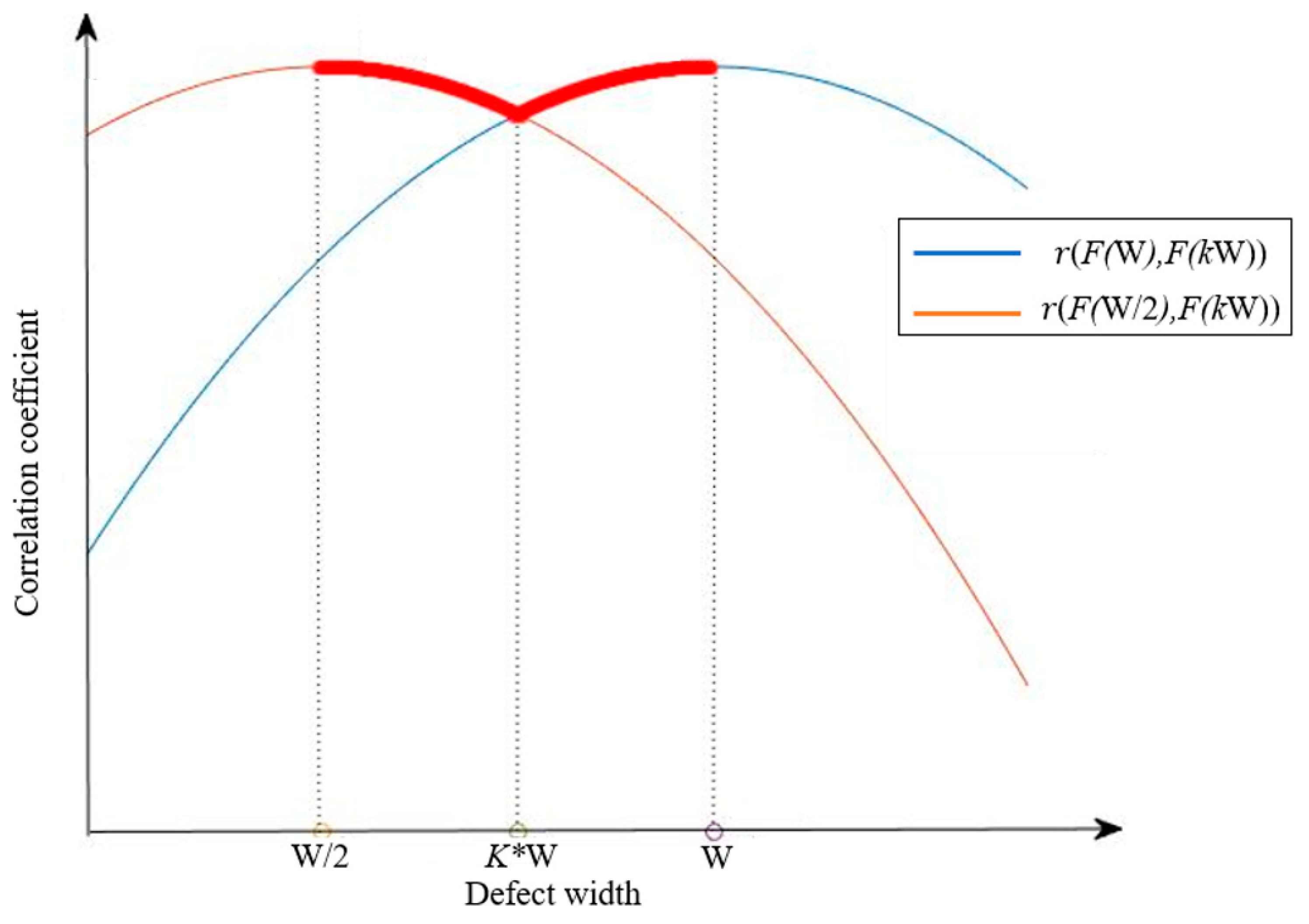
The core principle involves analyzing the correlation coefficient r between a reference template F(W) and its binary scale counterpart F(W/2) against intermediate-width templates F(kW) (0.5 < k < 1). Here, r(F(i), F(j)) quantifies the morphological similarity between templates F(i) and F(j). Theoretical analysis reveals that r(F(W), F(kw)) monotonically decays as k deviates from 1, while r(F(W/2), F(kW)) decays monotonically as k deviates from 0.5. Consequently, a critical width ratio k* must exist where r(F(W), F(k*W)) = r(F(W/2), F(k*W)), defining the optimal transition threshold. As illustrated in Figure 5, the blue curve represents the decay of r between F(W)and full-width basis functions, while the orange curve corresponds to F(W/2); the intersection (red) denotes the optimal solution k*.

By solving the equation r (F(W), F(kW)) = r (F(W/2), F(kW)), the critical ratio k* can be determined. As shown in Equation (8), where cov (x, y) is the covariance, var (x) is the variance, and H and ΔH in F(k*W) also vary with the ratio.

$$\begin{array}{c}{\mathrm{r}\left(\mathrm{F}\right(\mathrm{W}),\mathrm{F}(\mathrm{k}}^{*}\mathrm{W}\left)\right)={\displaystyle \frac{{\mathrm{Cov}\left(\mathrm{F}\right(\mathrm{W}),\mathrm{F}(\mathrm{k}}^{*}\mathrm{W}\left)\right)}{\sqrt{{\mathrm{var}\left(\mathrm{F}\right(\mathrm{W}\left)\right)\mathrm{var}\left(\mathrm{F}\right(\mathrm{k}}^{*}\mathrm{W}\left)\right)}}}\\ {\mathrm{r}\left(\mathrm{F}\right(\mathrm{W}/2),\mathrm{F}(\mathrm{k}}^{*}\mathrm{W}\left)\right)={\displaystyle \frac{{\mathrm{Cov}\left(\mathrm{F}\right(\mathrm{W}/2),\mathrm{F}(\mathrm{k}}^{*}\mathrm{W}\left)\right)}{\sqrt{{\mathrm{var}\left(\mathrm{F}\right(\mathrm{W}/2\left)\right)\mathrm{var}\left(\mathrm{F}\right(\mathrm{k}}^{*}\mathrm{W}\left)\right)}}}\end{array}$$

(8)

For any target width interval (Wmin, Wmax), the partitioning proceeds as follows: First, generate the initial template F(Wmax) using Wmax and its parameters, then compute the binary scale template F(Wmax/2). Solving the equation (F(Wmax), F(k*Wmax)) = r(F(k*Wmax), F(Wmax/2)) yields the critical ratio k* establishing that F(Wmax) covers the interval (kWmax, Wmax] while F(Wmax/2) covers (Wmax/2, k*Wmax]. This process recurses by setting Wmax/2 as the new Wmax. When the recursive process generates a binary scale template width (W/2) that is less than the minimum defect width observed in the dataset (Wmin), the iteration ceases. At this point, further binary partitioning is halted, and the current template width (W, the last width before termination) is used to cover all defect widths in the range [Wmin, W].

The selection of the minimum width threshold W for terminating the binary recursion and employing a single template is primarily driven by two key considerations: diminishing returns in morphological differentiation and practical engineering constraints. Continuing the binary partitioning below Wmin results in templates whose correlation coefficients with the template exhibit minimal decay, approaching 1.0. This indicates a negligible morphological distinction between these finer-scale templates, leading to minimal additional benefits in feature specificity. Moreover, the introduction of numerous highly similar templates would significantly increase computational overhead due to the need for parallel convolution, which is inefficient.

Ultimately, finite binary scale templates with optimized coverage ranges achieve complete coverage of continuous defect widths.

This method achieves continuous width coverage using minimal templates through recursive binary partitioning and critical ratio calculation. Each template operates exclusively within its optimal interval, reducing the number requiring concurrent computation or invocation. During convolutional network training—where image labels contain full defect width data—the binary-scale template optimization mechanism enhances features by: first, assigning each defect to its optimal template (e.g., F(Wmax) for (k*Wmax, Wmax], F(Wmax/2) for (Wmax/2, k*Wmax]) based on true width. Second, performing convolution using the matched kernel. For images with multiple defects of varying widths, feature enhancement applies individually to each defect’s minimum bounding rectangle. By ensuring every defect is processed by its morphologically closest kernel, this approach significantly boosts the precision and efficacy of feature extraction, optimizing training data enhancement.

3.4. Dynamic Threshold Segmentation via Bimodal Feature Distribution and 3σ Principle

Convolutional neural networks typically comprise a feature-extracting base layer and a classification-oriented top layer. The base layer generates feature values representing abstract image characteristics, whereas the top layer transforms these into class probabilities via nonlinear mapping. This study enhances features using adaptive templates fused with correlation coefficient decay, then feeds them into a CNN while replacing the top classification structure with a model that leverages the bimodal distribution of feature values. By applying 3σ extreme-value statistics, the model sets thresholds using the top 0.3% extreme values from the foreground feature peak.

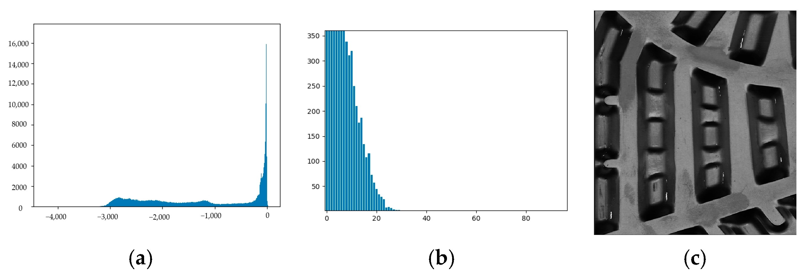
The bimodal distribution emerges from the distinct separation between background and defect feature responses in the CNN’s feature space, as illustrated in Figure 6. After adaptive template enhancement and convolutional processing, background pixels yield low-valued feature responses in receptive fields due to weak template correlation, forming the background peak; defect pixels generate high-valued responses via morphological matching, creating the foreground peak. A two-component Gaussian mixture model fits the feature histogram to determine both peaks’ means and standard deviations.

Derived from normal distribution statistics, the 3σ principle dictates that approximately 99.73% of values for a normally distributed variable fall within three standard deviations of the mean. Values beyond this range are statistically classified as extremes. In this article’s context, the focus centers on extreme-value points within the foreground peak of the feature distribution, previously modeled by the Gaussian mixture framework. Per the 3σ criterion, feature values exceeding μ + 3σ represent extreme high-value points in the foreground peak distribution, thus serving as candidate defect pixels.

The bimodal characteristic confirms feature values’ effectiveness as a defect similarity metric, while the 3σ principle establishes a mathematical framework for robust defect identification from this statistical distribution. This approach grounds the theory of representing defects through convolutional feature maxima upon quantifiable statistical regularities.

4. Experimental Results

This section first introduces the SUT-B1 dataset, then details implementation specifics and evaluation metrics, subsequently validates the detection model, and finally provides analysis and discussion of the corresponding experimental results.

4.1. Dataset

To validate the proposed algorithm’s efficacy, this study constructs the SUT-B1 microcrack image database, featuring microcrack defects measuring 0.29–0.88 mm in width. Images were captured in an actual production environment, as illustrated in Figure 7, where the acquisition system is mounted on an automated production line. The camera and lens are fixed to a gantry frame above the inspection platform at a working distance of 1185.11 mm, while the light source is positioned 35 mm above the conveyor. Plates advance via rollers, triggering image capture upon photoelectric switch activation; the light source illuminates synchronously with the camera’s exposure. The system employs a 16 k-pixel line-scan camera, a matched line-scan lens, and a tunnel lighting source.

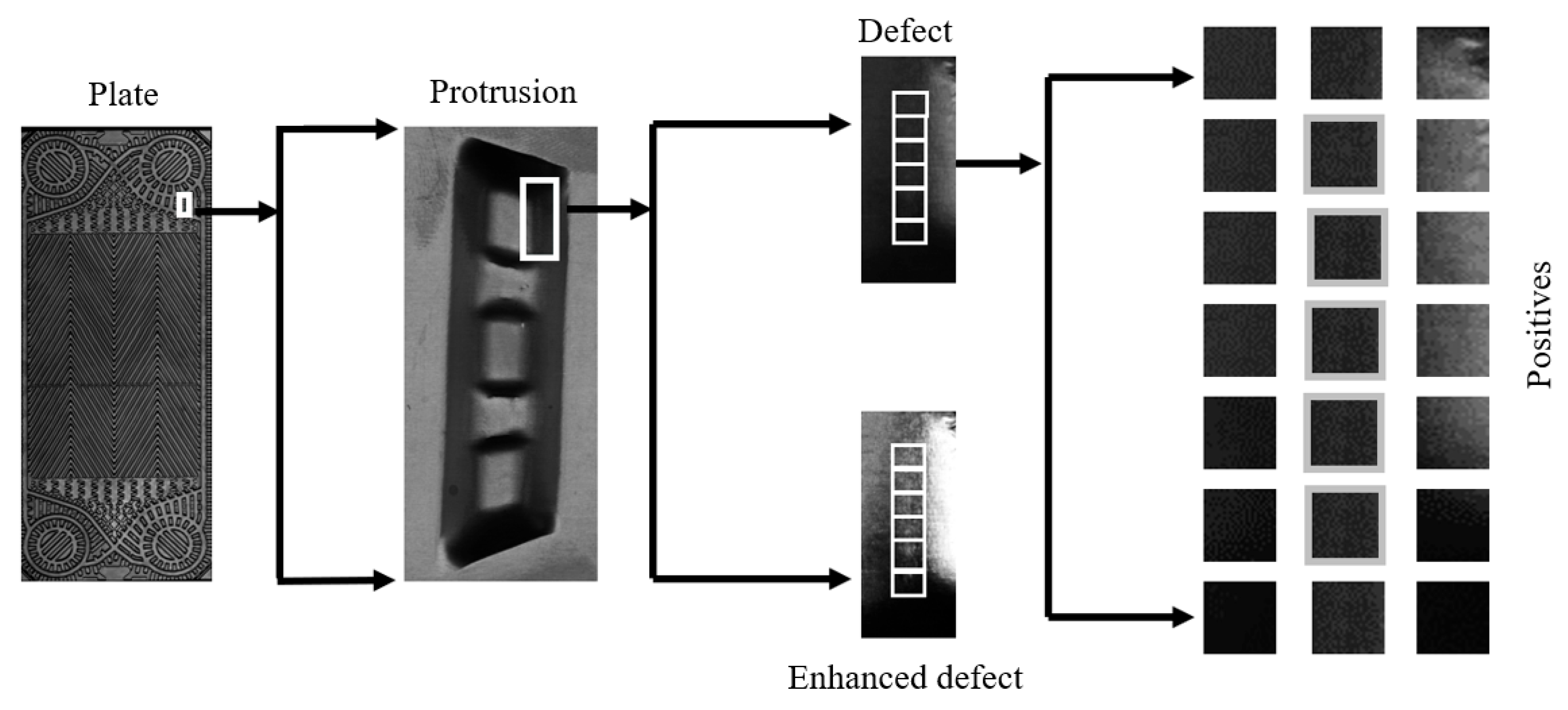
Training samples are generated by annotating defect regions, specifically by labeling bounding boxes around these areas and cropping them into fixed-size square images as positive training samples. Figure 8 sequentially presents the plate heat exchanger’s full structure, raised structural zones prone to defects, localized defect regions, and cropped positive sample images derived from bounding boxes.

Figure 9(a1,a2) displays actual defect instances in physical plate heat exchanger samples, while Figure 9(b1,b2) illustrates their corresponding bounding box annotations. This comparative visualization demonstrates the spatial correspondence between authentic defect morphology locations and annotated regions, concurrently validating that labeling results accurately reflect real defect characteristics.

During testing, an improved scanning window technique generates test samples to prevent edge defect truncation and missed detections caused by cropping. As illustrated in Figure 10, fixed-pixel strides slide along width and height axes. The window size accommodates the largest object defect entirely, while stride settings ensure the smallest defect is fully covered by at least one window—eliminating omission risks from excessive strides. This parametric configuration balances computational efficiency with detection coverage.

To enhance the model’s generalization capability and mitigate the risk of high variance associated with the limited sample size, this study introduces plate sheet images of the same material but different models to expand the dataset. New plate sheet models include: P10B (1000 mm × 407 mm), 02CG (993 mm × 250 mm), EA10B (995 mm × 373 mm), and U20B (169 mm × 610 mm). A total of 12 plate sheet images across these four models were collected. Data partitioning was performed at the plate sheet model level: 6 plate sheets were allocated to the training set, and the remaining 6 plate sheets to the test set. Following this expansion, the training set comprises 2483 data instances, containing 283 marked defects distributed across 134 data instances. The test set comprises 2813 data instances, containing 317 marked defects distributed across 158 data instances. This expansion strategy aims to increase the diversity (different sheet sizes) and quantity of samples, thereby improving the model’s generalization performance in broader scenarios.

To elucidate the data instance generation process, consider a P10B model plate sheet with an image size of 19,214 × 9777 pixels as an example. Data instances were generated using a sliding window approach. The window size was set to 650 × 650 pixels, with a sliding stride of 600 pixels. This ensured an overlap of 50 pixels between adjacent windows, guaranteeing that defects with the known maximum width of 21 pixels would be entirely contained within at least one window. Zero-padding was applied to the edge regions of the plate image when the remaining area was insufficient for a full window. The total number of data instances was calculated as follows: the number of rows = ceil(19,214/600) = 33, the number of columns = ceil(9777/600) = 17, resulting in 561 data instances generated from the P10B sheet. Among these, 22 data instances contained defects, and 539 contained no defects. Each defect has a corresponding label image, as shown in Figure 9(b1,b2). This label image is a binary image spatially aligned with the data instance. Performing a skeletonization operation on the label image, skeleton information with a width of one pixel and an unfixed length is obtained. In data instances containing defects, take some skeleton coordinate points are taken as the center to generate positive sample images with a width of 13 pixels on both the left and right sides. Since the training and test sets originate from distinct plate sheets, and the generation of data instances is performed independently on the complete images of each sheet, no overlapping data instances exist between the training and test sets, thus ensuring strict independence.

All experiments were conducted on a Windows 11 system with a 2.6 GHz Intel Core i7-13650HX CPU and an NVIDIA RTX 5060 GPU. Python 3.8 served as the programming framework. Model training employed mini-batch stochastic gradient descent with a momentum factor of 0.9, an initial learning rate of 0.01, and 5-fold decay every 50 epochs.

4.2. Evaluation Metrics

The model outputs pixels within the extremely high-value region (top 0.3%) of feature distributions. After identifying candidate defect pixels based on the 3σ principle, post-processing is performed to filter out discrete noise and form the core defect regions. First, connected component labeling is applied to the candidate pixels, aggregating pixels within an 8-connected neighborhood into distinct regions. The area of each connected component is calculated, and components with an area below a threshold of 4 pixels are removed. The remaining components are merged into a unified region. Subsequently, a morphological opening operation is executed using a disk-shaped structuring element with a radius of 1 pixel, applied iteratively once. The erosion operation is performed first to eliminate minor protrusions along region boundaries, followed by a dilation operation to restore the core defect areas affected by erosion. Our detection criterion requires only that the Intersection over Union (IoU) between a predicted target region and a defect instance be greater than zero to consider the defect detected. This is because the primary focus of the detection task is on the presence of defects; as long as a predicted region intersects with a defect, that defect is considered detected. Accordingly, each predicted object is matched against all defect instances; intersections meeting this IoU > 0 criterion are marked as true positives, with matched pairs subsequently removed. Unmatched predictions become false positives, while unmatched defects are false negatives. Equations (9)–(13) formalize these metrics:

$$\mathrm{R}=\mathrm{TP}/\mathrm{N}$$

(9)

$$\mathrm{P}=\mathrm{TP}/(\mathrm{TP}+\mathrm{FP})$$

(10)

$$\mathrm{F}1=2\times (\mathrm{P}\times \mathrm{R})/(\mathrm{P}+\mathrm{R})$$

(11)

$$\mathrm{F}\mathrm{P}\mathrm{B}=\mathrm{F}\mathrm{P}/{\mathrm{N}}_{\mathrm{b}}$$

(12)

$$\mathrm{M}\mathrm{D}\mathrm{B}=\mathrm{F}\mathrm{N}/{\mathrm{N}}_{\mathrm{b}}$$

(13)

True positives (TP) denote detected defects, false positives (FP) represent misidentified defects, and false negatives (FN) indicate undetected defects. The total defect count (N) equals the aggregated instances in the test set. The number of corrugated boards in the test set is (N_b), with false positives per board denoted as (FPB) and missed detections per board denoted as (MDB). The evaluation criteria are: recall (R); precision (P); F1 score (F1).

4.3. Detection Results

The test was conducted on the data from the test set in Section 4.1, and the obtained parameters are shown in

Table 1. The result of the proposed method.

R (%)	P (%)	F1 (%)	FPB	MDB
83.59	80.55	81.98	10.67	8.67

.

The dataset exhibits defect widths ranging from 7 to 21 pixels, heights from 7 to 46 pixels, and endpoint grayscale differences from 1 to 22 pixels. To prevent excessive feature compression during binary downsampling, three adaptive templates were selected: the maximum-width template (Wmax = 21, denoted F(Wmax)) representing defects with W = 21, H = 38, ΔH = 18; the first binary downsampling template (Wmax/2 = 11, F(Wmax/2)) simulating W = 11, H = 24, ΔH = 10; and the minimum-width template (Wmin = 7, F(Wmin)) corresponding to W = 7, H = 8, ΔH = 3. Their continuous functions are formulated in Equations (14)–(16).

$${\mathrm{F}(\mathrm{W}}_{\max }) =-0.26{\mathrm{x}}^2+6.24\mathrm{x}-27.81$$

(14)

$${\mathrm{F}(\mathrm{W}}_{\max /2}) =-0.62{\mathrm{x}}^2+7.70\mathrm{x}-17.35$$

(15)

$${\mathrm{F}(\mathrm{W}}_{\min }) =-0.52{\mathrm{x}}^2+4.10\mathrm{x}-5.63$$

(16)

Substituting the templates into Equation (8) yields scaling factors k = 0.728 between F(Wmax) and F(Wmax/2), and k = 0.788 between F(Wmax/2) and F(Wmin). With 11 × 0.788 rounded up to 9 and 24 × 0.728 rounded up to 18, defect enhancement is applied as follows: defects within the [7, 9] pixel width range use F(Wmin), those within the [10, 17] range employ F(Wmax/2), and defects in the [18, 24] range utilize F(Wmax).

After enhancing the dataset using the described templates, convolutional network training was conducted. Analysis of the test images’ bimodal feature distribution identified the top 0.3% extreme values at the foreground peak. Final validation followed the evaluation metrics framework.

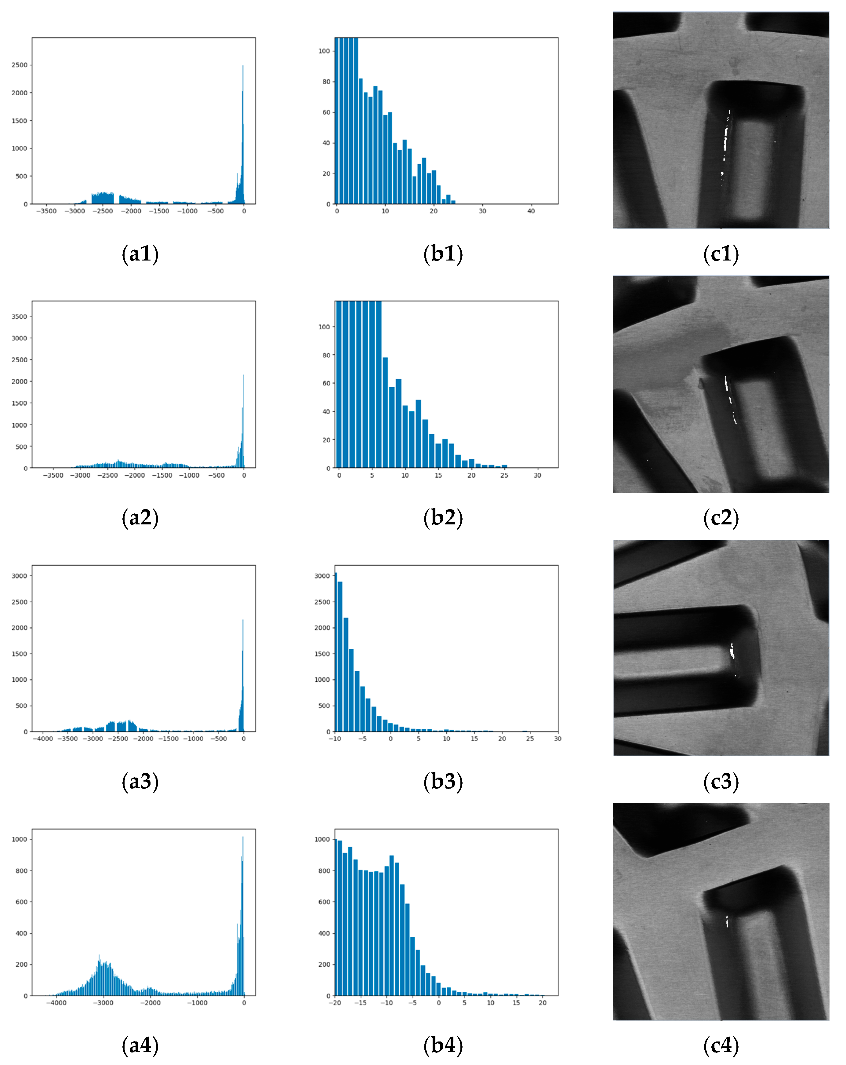
Figure 11 and Figure 12 demonstrate the proposed algorithm’s detection performance in multi-defect coexistence and single-defect scenarios, respectively. To characterize feature distribution in defect regions, histograms visualize convolutional layer outputs with the x-axis representing feature values and the y-axis indicating corresponding frequencies—typically exhibiting foreground and background peaks. Figure 11 presents multi-defect results: Figure 11a displays the feature distribution (range [−4249, 32]), Figure 11b highlights extreme high-value regions identified via 3σ thresholding (range [12, 32]), while Figure 11c visualizes the spatial distribution of these extreme features. Further analysis in Figure 12 examines four defect regions processed through adaptive template enhancement and CNN: Figure 12(c1–c4) visualize spatial distributions of extreme features (white areas) in single-defect images; Figure 12(a1–a4) present feature value images; Figure 12(b1–b4) show feature intervals selected via the 3σ principle from foreground peaks. These results collectively validate the algorithm’s effectiveness across diverse defect scenarios.

5. Discussion

To comprehensively evaluate the proposed method’s performance across multiple dimensions, systematic experimental analyses were conducted. Firstly, comparative studies against small object detection models demonstrated the advantages of our approach in resource-constrained environments. Subsequently, benchmarking against receptive field optimization modules validated the effectiveness of parametric adaptive template generation and binary scale optimization for feature enhancement. Further investigation into sliding window stride configurations revealed the optimal balance between detection coverage and computational efficiency. Additionally, analysis of defect width handling and computational cost under multi-template parallel inference provided insights into practical deployment considerations. Moreover, end-to-end throughput and industrial robustness tests confirmed the method’s suitability for real-world applications. Finally, sensitivity analysis of bimodal distribution characteristics and threshold parameters established the reliability of the proposed segmentation strategy.

5.1. Comparison with Small Object Detection Models

Because of the lack of comparison with industrial-grade frameworks, we conducted supplementary experiments comparing our proposed algorithm against three representative small object detection models optimized for resource-constrained environments: YOLOv8-nano, EfficientDet-Lite, and NanoDet-Plus. YOLOv8-nano, the latest iteration of the YOLO series, employs an efficient backbone network and detection head design aimed at maximizing inference speed while minimizing resource consumption. EfficientDet-Lite0, the lightest variant within the EfficientDet-Lite series, is a lightweight adaptation of the EfficientDet architecture. It utilizes a shared feature network and a compound scaling strategy to balance efficiency and accuracy, emphasizing deployment performance on edge devices. NanoDet-Plus-m-320, the lightest variant within the NanoDet-Plus series, is a lightweight model specifically designed for small object detection. It employs an anchor-free mechanism to reduce memory footprint. The comparative experiments were performed under identical experimental settings. The results are presented in

Table 2. Detection results of different small object detection models.

Method	R (%)	P (%)	F1 (%)	FPB	MDB
Ours	83.59	80.55	81.98	10.67	8.67
YOLOv8-nano	78.04	80.98	79.99	9.67	11.67
EfficientDet-Lite	85.55	77.00	80.49	13.50	7.67
NanoDet-Plus	46.75	91.13	61.95	2.17	28.17

.

Analysis of the results reveals specific limitations in the competing models when applied to our microcrack detection task: YOLOv8-nano suffers from insufficient feature extraction capability for small targets in shallow layers due to multiple downsampling operations, resulting in an R of 78.04%. EfficientDet-Lite0’s feature fusion process involves seven blocks, leading to confusion between defect features and background noise. This significantly degrades P, achieving only 77.00%. NanoDet-Plus-m-320’s learning process heavily relies on model thinning techniques for feature selection. While promoting lightweight design, this constrains its multi-scale feature fusion capability, causing the model to overfit in our small sample scenario. Consequently, its R drops to a low 46.75%.

5.2. Comparison with Receptive Field Optimization Model

To validate the effectiveness of parametric adaptive template generation and binary scale optimization for feature enhancement, this study compares their performance against representative modules specifically designed for optimizing network receptive fields—including ASPP, RFB, and DRConv—which capture contextual information across different scales or spatial positions to enhance model performance. The experimental results are shown in

Table 3. Detection results of different receptive field optimization models.

Method	R (%)	P (%)	F1 (%)	FPB	MDB
Ours	83.59	80.55	81.98	10.67	8.67
ASPP	53.00	66.40	59.70	14.17	24.83
RFB	73.82	76.22	75.04	12.16	13.83
DRConv	78.23	78.73	78.23	11.17	11.50

.

The ASPP module employs dilated convolution to capture discrete scale information but struggles to adapt to the continuous width variations of microcracks, resulting in insufficient width adaptability and increased missed detections. While the RFB module enhances feature diversity through multi-branch receptive fields, it introduces interference for small linear features such as microcracks, elevating false positives. DRConv’s dynamic kernel weight learning tends to cause overfitting in limited-sample datasets, confusing targets with background.

5.3. Comparison with Different Strides of the Sliding Window

To investigate the impact of sliding window stride on detection metrics, we systematically tested three stride configurations under the condition of a fixed window size of 64 × 64 pixels, namely 32 pixels, 64 pixels, and 128 pixels. Among them, the 32-pixel stride is the parameter adopted by the algorithm in the model. The detection results under different strides are shown in

Table 4. Detection results of different strides of the sliding window.

Stride	R (%)	P (%)	F1 (%)	FPB	MDB
32 (Ours)	83.59	80.55	81.98	10.67	8.67
64	79.18	83.67	81.33	8.17	11.00
128	56.47	86.06	68.43	4.83	23.00

.

Step size = 64 pixels, meaning when the step size equals the window size, there is no overlap between adjacent windows. Compared to the step size = 32 scenario, this configuration results in a decrease in R. The reason is that some defects may be split into two adjacent windows. When the step size is smaller than the window size, it ensures that the largest defect remains within one window. When the step size equals the window size, a defect may belong to two windows. If the upper and lower parts of a linear defect belong to two windows, the impact is relatively small; if the left and right parts of a linear defect belong to two windows, the impact is greater. Although the reduction in overlapping areas decreases the duplicate counting of false positives, thereby improving P, the F1 score is still lower than that of the step size = 32 configuration, indicating that the accuracy improvement cannot compensate for the loss in recall rate. Step size = 128 pixels, meaning the step size is larger than the window size, results in significant gaps between sampling windows. This sparse coverage leads to a decrease in R. Some defects, either partially or entirely, fall within these gaps, causing missed detections. Although the P remains relatively high, the F1 score is still lower than that of the step size = 32 scenario, confirming that this configuration is not suitable for reliable defect detection.

5.4. Analysis of Defect Width Handling and Computational Cost Under Multi-Template Parallel Inference

The microcrack defects targeted in this study specifically refer to their early-stage morphology prior to macroscopic cracking. Within metallic materials, the presence of microscopic defects leads to stress concentration in their vicinity under external loading. When the tip stress intensity exceeds the material’s fracture toughness, the defect propagates, forming a macroscopically visible crack. Conversely, clusters of microcracks form. Examining the difference between these states under local magnification, light passes through the gap formed by a cracked plate section, resulting in no reflected light. In contrast, for an uncracked plate section, light fails to pass through the gap, leading to reflected light. Consequently, the microcrack defects addressed in this research manifest visually as linear regions of grayscale anomaly within a specific width range. This limited, small-scale width range provides the physical basis for constructing a binary-scale template library to cover it. However, during the inference stage, for any given local region under inspection, the presence of a defect and its precise width information are a priori unknown. Figure 13 illustrates the cracked defect and microcrack defect, demonstrating that the width of microcracks is limited. Only when external force is continuously applied does the defect area extend, forming a cracking defect. Figure 13(a1,a2) present the images of different types of defects; Figure 13(b1,b2) show the defect longitudinal grayscale distribution curve.

To address the challenge of unknown defect width during inference, our method adopts a “Multi-Template Parallel Convolution” strategy. Specifically, during inference, the input image is simultaneously convolved with all pre-generated binary-scale templates covering the target width range. This operation produces multiple corresponding feature maps. These feature maps are subsequently fed into a convolutional network for fusion and feature learning. Taking the test image of plate P10B as an example, processing the entire plate directly is prone to causing insufficient memory. Therefore, the plate is first subdivided into 561 sub-images of size 650 × 650 pixels, following the same cropping method used for the training set. Multi-scale template convolution is then applied to each sub-image. For each sub-image, the computational cost of convolution with a single template is 1.48 s in time and 8.97 MB in memory. In contrast, the parallel convolution using multiple templates incurs a time cost of 4.65 s and a memory footprint of 21.29 MB per sub-image.

5.5. End-to-End Throughput Analysis and Industrial Robustness Validation

To evaluate the industrial applicability of the proposed algorithm, end-to-end throughput and robustness against typical interference scenarios were systematically tested.

The test set comprised six large plate sheets of varying sizes. The total processing time from inputting full-sheet images to outputting all defect information was 2415 s, averaging 402.5 s per sheet. The combined area of the six sheets was 1,966,750 mm², yielding a detection speed of 814 mm² per second. During inference, peak GPU VRAM usage was monitored at 8.6 GB, reflecting computational resource requirements.

To systematically evaluate the robustness and anti-interference capability of the proposed algorithm in complex industrial environments, this study constructed a data augmentation scheme that includes three types of interference simulations to mimic typical interference scenarios in actual production. The first type involves simulating oil contamination by adding random dark block-like regions, representing scenarios where the surface of the plate is partially obscured by contaminants such as cooling fluid and lubricating oil. The second type involves adding Gaussian noise to simulate electronic noise generated by image sensors under abnormal temperature or abnormal lighting conditions. The third type involves adding random perturbations to brightness and contrast to simulate changes in illumination caused by vibrations of light sources on the production line or different reflectance on the plate surface. New test plates are generated through the aforementioned augmentation methods to verify the industrial scalability of the algorithm. The visual effects of defects under different interferences are shown in Figure 14, where Figure 14(a1–a4) sequentially displays the original data, simulated oil stain, Gaussian noise, and illumination perturbation.

Using the aforementioned interference images, tests were conducted without altering any parameters. The results are presented in

Table 5. Detection results of anti-interference ability test.

Interference	R (%)	P (%)	F1 (%)	FPB	MDB
Orignal	83.59	80.55	81.98	10.67	8.67
Simulated Oil Stain	80.44	80.70	80.55	10.17	10.33
Gaussian Noise	77.29	79.03	77.48	10.83	12.00
Illumination Perturbation	83.59	78.87	81.30	11.83	8.67

. Under oil contamination stain, there was no impact on P, but R decreased. This indicates that physical obstruction caused the grayscale distribution characteristics of microcracks to be submerged under the low grayscale values of oil contamination, resulting in missed detections. Light disturbance had no effect on R but only reduced P. This suggests that under varying light intensity conditions, the linear grayscale differences in some false detection areas were amplified, leading to false detections. Under Gaussian noise conditions, detection performance declined, but no significant failures occurred, demonstrating its robustness for engineering deployment.

5.6. Robustness of Bimodal Distribution and Sensitivity of Threshold Parameters

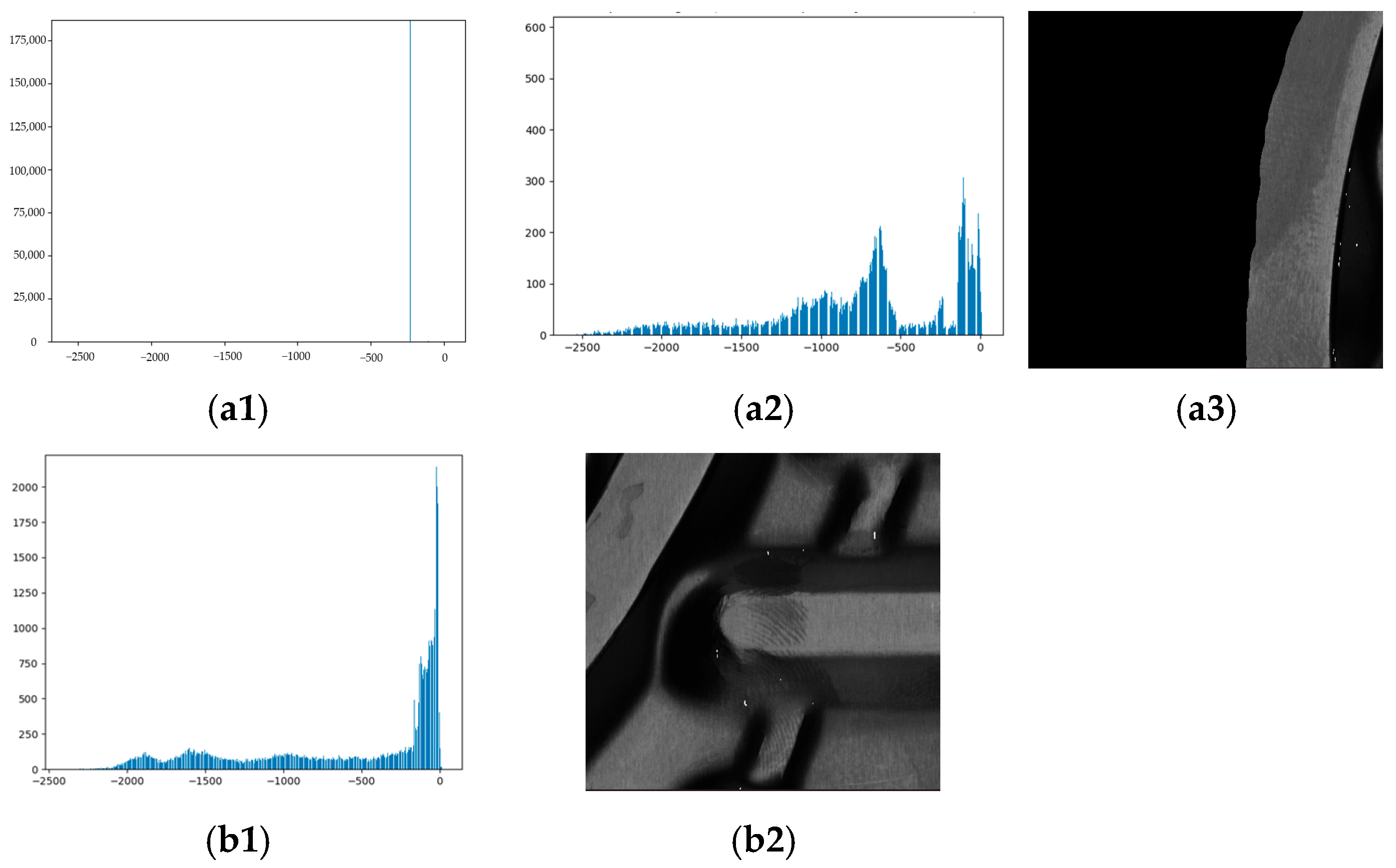
Regarding the bimodal distribution characteristics of the feature images, it is important to note that not all test images exhibit a pronounced bimodal distribution. To verify this, we processed images containing plate edges with backgrounds and high-noise images with fingerprint-like textures, observing the resulting feature distributions. Figure 15(a1) illustrates the feature distribution of a plate edge image. Due to the presence of extensive structurally repetitive background regions in the plate edge image, their consistent convolutional responses result in feature values being highly concentrated in a sharp, prominent peak. To reveal the distribution of the remaining feature values, Figure 15(a2) displays the distribution after removing this peak point, and Figure 15(a3) shows the result after applying the 3σ threshold. Figure 15(b1) presents the bimodal distribution feature map of a high-noise image containing fingerprint-like textures, and Figure 15(b2) shows the result after the 3σ thresholding. In these cases, the thresholded results manifest as spatially discrete noise points. These responses can be effectively removed by subsequent filtering and morphological operations. This indicates that the post-processing stage of the method possesses a certain fault tolerance capability, enabling it to filter out non-defect responses.

To address the sensitivity issue of the 3σ threshold strategy, a sensitivity experiment was conducted. Figure 16 presents the distribution of feature points corresponding to the foreground peak across different threshold intervals for a representative detection image. For clarity, the images in the article have undergone contrast enhancement. Figure 16(a1–a4), respectively, illustrate the feature point distributions for the top 0.1%, 0.1–0.3%, 0.3–0.5%, and 0.5–1% intervals, respectively. To clearly visualize the final detection results, detected defects are marked with red bounding boxes, missed defects with blue boxes, and false positives with green boxes. As observed, for a total of 13 defects, the 0.1% threshold resulted in TP = 2, FP = 0, FN = 11. The 0.3% threshold resulted in TP = 11, FP = 3, and FN = 2. The 0.5% threshold resulted in TP = 11, FP = 4, and FN = 2. The 1% threshold resulted in TP = 13, FP = 0, and FN = 12.

The experiment demonstrates that a threshold as low as 0.1% is nearly ineffective for defect detection. While a 1% threshold detects all defects, it incurs a high rate of false positives. Within the 0.3% to 0.5% threshold interval, similar detection outcomes are achieved, with the 0.5% threshold yielding only one additional false positive compared to 0.3%.

This sensitivity experiment validates the critical impact of threshold selection on detection performance. Excessively low thresholds increase the risk of missed detections, while excessively high thresholds elevate false positives. The 0.3–0.5% interval demonstrates a favorable balance point. However, considering the inherent variability in lighting, noise, and background conditions in real-world industrial environments, a fixed threshold may not be optimal. Future research could explore adaptive threshold selection mechanisms, such as dynamically adjusting the percentage threshold based on the characteristics of each image’s feature value distribution, to further enhance the method’s robustness under varying operating conditions.

6. Conclusions

To address challenges in industrial microcrack detection, including morphological diversity, continuous width variations, and dynamic threshold segmentation, this paper proposes a detection framework integrating parametrically adaptive template generation, binary scale optimization, and convolutional network feature value segmentation. By establishing a quantitative mapping model between defect morphological parameters (width, height, endpoint grayscale difference) and convolution kernel functions, morphology-driven feature enhancement is achieved. A binary recursive mechanism, designed based on template correlation coefficient decay characteristics, enables finite templates to cover continuous width ranges. Combining bimodal feature distribution modeling with extreme value statistical theory, an adaptive threshold segmentation strategy is constructed. This approach demonstrates robust detection performance in industrial small sample scenarios, outperforming mainstream convolutional network models and classical linear detection methods, providing an effective solution for industrial inspection.