Physics-Informed Neural Network for Denoising Images Using Nonlinear PDE

Abstract

Noise remains a persistent limitation in coherent imaging systems, degrading image quality and hindering accurate interpretation in critical applications such as remote sensing, medical imaging, and non-destructive testing. This paper presents a physics-informed deep learning framework for effective image denoising under complex noise conditions. The proposed approach integrates nonlinear partial differential equations (PDEs), including the heat equation, diffusion models, MPMC, and the Zhichang Guo (ZG) method, into advanced neural network architectures such as ResUNet, UNet, U2Net, and Res2UNet. By embedding physical constraints directly into the training process, the framework couples data-driven learning with physics-based priors to enhance noise suppression and preserve structural details. Experimental evaluations across multiple datasets demonstrate that the proposed method consistently outperforms conventional denoising techniques, achieving higher PSNR, SSIM, ENL, and CNR values. These results confirm the effectiveness of combining physics-informed neural networks with deep architectures and highlight their potential for advanced image restoration in real-world, high-noise imaging scenarios.

1. Introduction

Image denoising is a crucial task in image processing aimed at removing noise while preserving the underlying structures [1,2]. As high-resolution digital imagery becomes increasingly accessible, especially with novel modalities such as single-pixel imaging (SPI) [3,4], UAV or SAR Images [5,6], and other computer image applications, there is a growing demand for denoising algorithms that deliver high effectiveness and computational efficiency. In recent years, deep learning-based approaches have shown superior performance in image denoising, surpassing traditional hand-made methods [7]. These approaches employ convolutional neural networks (CNNs) to learn the mapping between noisy and clear from noisy to clean images, training on large datasets of paired noisy–clean difference between the network output and the corresponding clean image [8].

One of the key advantages of deep learning-based denoising methods is their ability to learn complex [9], nonlinear relationships between noisy and clean image patches [10,11]. This enables networks to capture both local and global image structures and patterns, resulting in more accurate and visually pleasing denoising results (see Table 1). Image priors [12], including nonlocal self-similarity (NSS) models [13], median filters [14], sparse models [15], gradient models [16], Markov models [17], BM3D [18], LSSC [19], NCSR [20], and WNNM [21], address the challenge of noise removal. More recently, deep learning-based denoising models, such as standard CNNs [22], residual networks (ResNets) [23], and generative adversarial networks (GANs) [24], have emerged as effective solutions. The standard CNN model learns a direct mapping from noisy to clean images, while the ResNet model uses skip connections to learn residual mappings, resulting in more efficient training and improved denoising performance. GAN-based models further enhance denoising by incorporating a generator that produces denoised images and a discriminator that differentiates between real and generated images, leading to more realistic and visually consistent results [24,25].

Physics-informed neural networks (PINNs) have emerged as a novel approach in artificial intelligence [26], particularly by using partial differential equations (PDEs) for efficient image denoising [27]. PDE-based models such as heat diffusion [28], Perona–Malik (PM) [29], MPMC [30], and the Black-Zhichang Guo model [31] are effective in addressing noise reduction in images. In the PINN framework, a neural network is utilized to approximate the solution of a PDE by minimizing a loss function that includes terms representing the mismatch of the residual PDE and its boundary conditions. The nonlinearity of PDEs and the varying boundary conditions do not pose significant challenges when employing neural networks, offering a distinct advantage over traditional numerical methods. However, integrating PDEs into deep learning frameworks also introduces challenges, including balancing accuracy and stability, managing computational complexity, and ensuring interpretability [32]. Many existing approaches address these issues only partially, leaving room for improvement in terms of generalization, computational efficiency, and preservation of fine-scale structures.

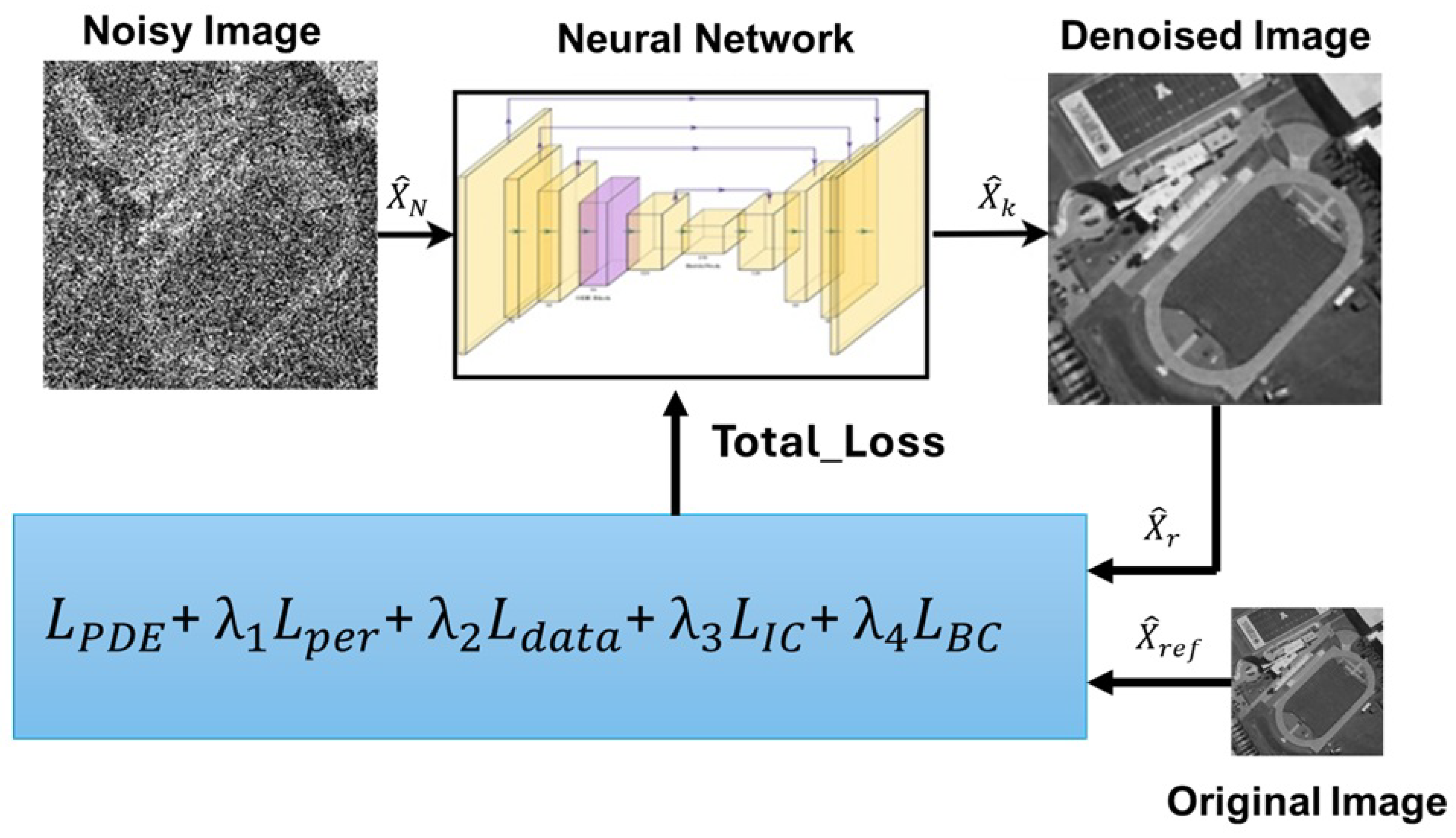
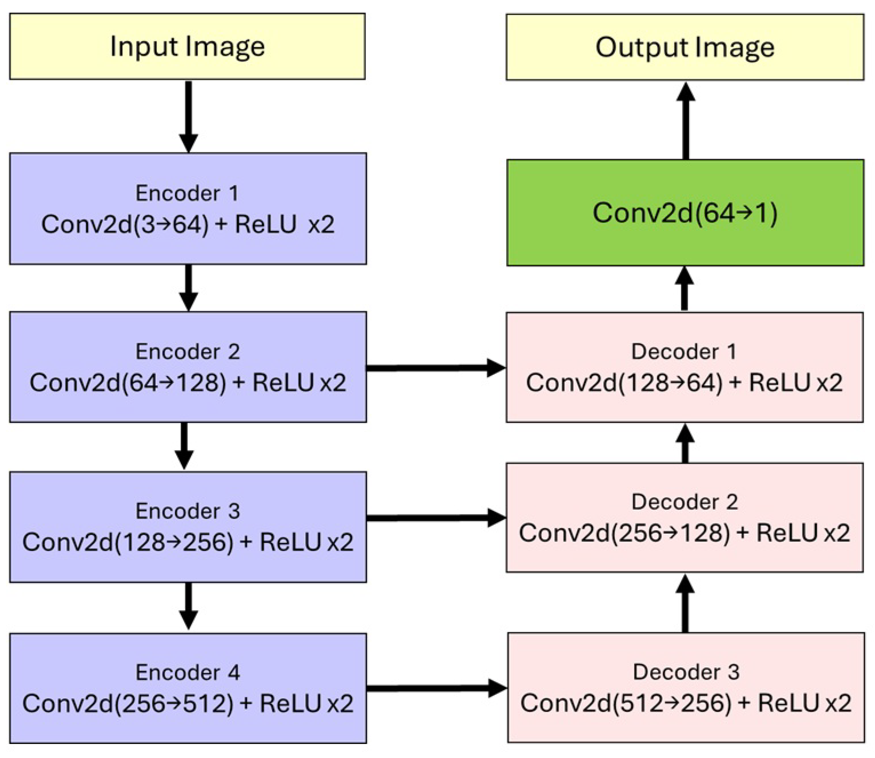
This work presents a physics-informed deep learning framework that couples nonlinear PDE priors—heat, diffusion-based regularization, Mean Curvature Motion (MPMC), and the Zhichang Guo (ZG) model—with modern denoising backbones including ResUNet, UNet, U2Net, and Res2UNet. We focus on these four PDEs because they offer complementary denoising behavior while remaining computationally predictable and suitable for future FPGA/embedded-GPU deployment [33,34]. Specifically, heat provides a stable isotropic baseline, diffusion introduces edge-aware anisotropy, MPMC enforces curvature-driven geometric smoothing, and ZG improves robustness under speckle and other multiplicative degradations.

By embedding physical constraints directly into the network training process, the proposed method improves denoising performance, preserves fine structural details, and reduces dependence on large-scale labeled datasets. This hybrid approach combines the interpretability and stability of PDE-based modeling with the representational power of deep learning, offering a robust and scalable solution for image denoising in challenging noise environments. To rigorously assess the performance of the framework, a comprehensive set of evaluation metrics is used, including the peak signal-to-noise ratio (PSNR), the structural similarity index measure (SSIM), the equivalent number of looks (ENL), and the contrast-to-noise ratio (CNR). Our experiments consistently achieve PSNR values greater than 20 dB and SSIM values greater than 0.5, demonstrating the effectiveness of the model in enhancing image quality while maintaining computational efficiency.

The main contributions of this work are summarized as follows:

• The integration of physics-informed neural networks (PINNs) with PDE-based models for effective image denoising leverages physical priors to enhance noise suppression and structural preservation.
• This study introduces a rigorous and diverse set of evaluation metrics for denoising in remote sensing imagery, spanning pixel-level fidelity and perceptual quality.
• The proposed framework demonstrates superior performance compared to classical denoising algorithms and existing deep learning-based methods, achieving higher image quality and robustness across multiple datasets.

Table 1. Overview of the main advantages and drawbacks of the implemented denoising approaches.

Method	Advantages	Drawbacks
Supervised CNN [35]	High reconstruction quality with sufficiently large labeled training sets.	Requires extensive paired datasets; weaker generalization outside the training domain.
Self-supervised CNN [36]	Training does not require paired clean labels; it can learn directly from noisy data.	May exhibit residual bias and relies on masking/noise assumptions that can be violated.
Wavelet/Sparse [37]	Often excellent PSNR/SSIM for additive Gaussian noise; interpretable transform-domain representation.	Can leave granular residue for speckle-like noise; requires careful parameter tuning.
Score-based diffusion [38]	Naturally integrates explicit forward noise models; very strong perceptual quality.	Computationally demanding due to long sampling chains with many denoising steps.
Variance-stabilized PDE [39]	Simple pipeline combining variance-stabilizing transform and PDE evolution; fast and lightweight.	Inverse-VST can introduce bias; performance degrades for strongly spatially varying noise.
Nonlocal PDE/NL-TV [40]	Preserves fine textures and details by exploiting nonlocal similarities; texture-aware regularization.	Sensitive to patch and hyper-parameter choices; typically higher runtime.
Classical PDE [41]	Conceptually simple, interpretable, and numerically stable with low computational cost.	Parameter sensitive and prone to over-smoothing fine structures and textures.
PINN–PDE [42]	Physics-informed formulation enables adaptation across sensors with limited retuning.	More complex training procedure and higher computational cost than analytical PDE solvers.
Transformer-based denoisers [43]	Easy to add noise-level maps, prompts, or multi-scale features.	Can overfit to training noise statistics; may generalize poorly to unseen sensors/artifacts.
Diffusion-model denoisers [44]	Robust when noise/artifacts are heavy or complex (with good conditioning).	Expensive to train. Strong generative prior may introduce plausible but incorrect details—bad.
DIP-TV [45]	Can work reasonably even when the noise model is not well specified.	DIP can start fitting noise; results depend on stopping criterion/hyperparameters.
SwinIR [46]	Strong on PSNR/SSIM, preserves edges and textures well with long-range context.	Needs supervised (or well-designed self-supervised) training; may generalize poorly to unseen sensors/noise statistics.
DDPMs [47]	Can handle complex noise/artifacts when properly conditioned.	Many denoising steps; even accelerated samplers can be heavy.
DDRM [48]	Designed for restoration/inverse problems; can incorporate the measurement/degradation model more directly than plain DDPM denoising.	Inference remains multi-step, often similar order to diffusion sampling.

Table 1. Overview of the main advantages and drawbacks of the implemented denoising approaches.

Method	Advantages	Drawbacks
Supervised CNN [35]	High reconstruction quality with sufficiently large labeled training sets.	Requires extensive paired datasets; weaker generalization outside the training domain.
Self-supervised CNN [36]	Training does not require paired clean labels; it can learn directly from noisy data.	May exhibit residual bias and relies on masking/noise assumptions that can be violated.
Wavelet/Sparse [37]	Often excellent PSNR/SSIM for additive Gaussian noise; interpretable transform-domain representation.	Can leave granular residue for speckle-like noise; requires careful parameter tuning.
Score-based diffusion [38]	Naturally integrates explicit forward noise models; very strong perceptual quality.	Computationally demanding due to long sampling chains with many denoising steps.
Variance-stabilized PDE [39]	Simple pipeline combining variance-stabilizing transform and PDE evolution; fast and lightweight.	Inverse-VST can introduce bias; performance degrades for strongly spatially varying noise.
Nonlocal PDE/NL-TV [40]	Preserves fine textures and details by exploiting nonlocal similarities; texture-aware regularization.	Sensitive to patch and hyper-parameter choices; typically higher runtime.
Classical PDE [41]	Conceptually simple, interpretable, and numerically stable with low computational cost.	Parameter sensitive and prone to over-smoothing fine structures and textures.
PINN–PDE [42]	Physics-informed formulation enables adaptation across sensors with limited retuning.	More complex training procedure and higher computational cost than analytical PDE solvers.
Transformer-based denoisers [43]	Easy to add noise-level maps, prompts, or multi-scale features.	Can overfit to training noise statistics; may generalize poorly to unseen sensors/artifacts.
Diffusion-model denoisers [44]	Robust when noise/artifacts are heavy or complex (with good conditioning).	Expensive to train. Strong generative prior may introduce plausible but incorrect details—bad.
DIP-TV [45]	Can work reasonably even when the noise model is not well specified.	DIP can start fitting noise; results depend on stopping criterion/hyperparameters.
SwinIR [46]	Strong on PSNR/SSIM, preserves edges and textures well with long-range context.	Needs supervised (or well-designed self-supervised) training; may generalize poorly to unseen sensors/noise statistics.
DDPMs [47]	Can handle complex noise/artifacts when properly conditioned.	Many denoising steps; even accelerated samplers can be heavy.
DDRM [48]	Designed for restoration/inverse problems; can incorporate the measurement/degradation model more directly than plain DDPM denoising.	Inference remains multi-step, often similar order to diffusion sampling.

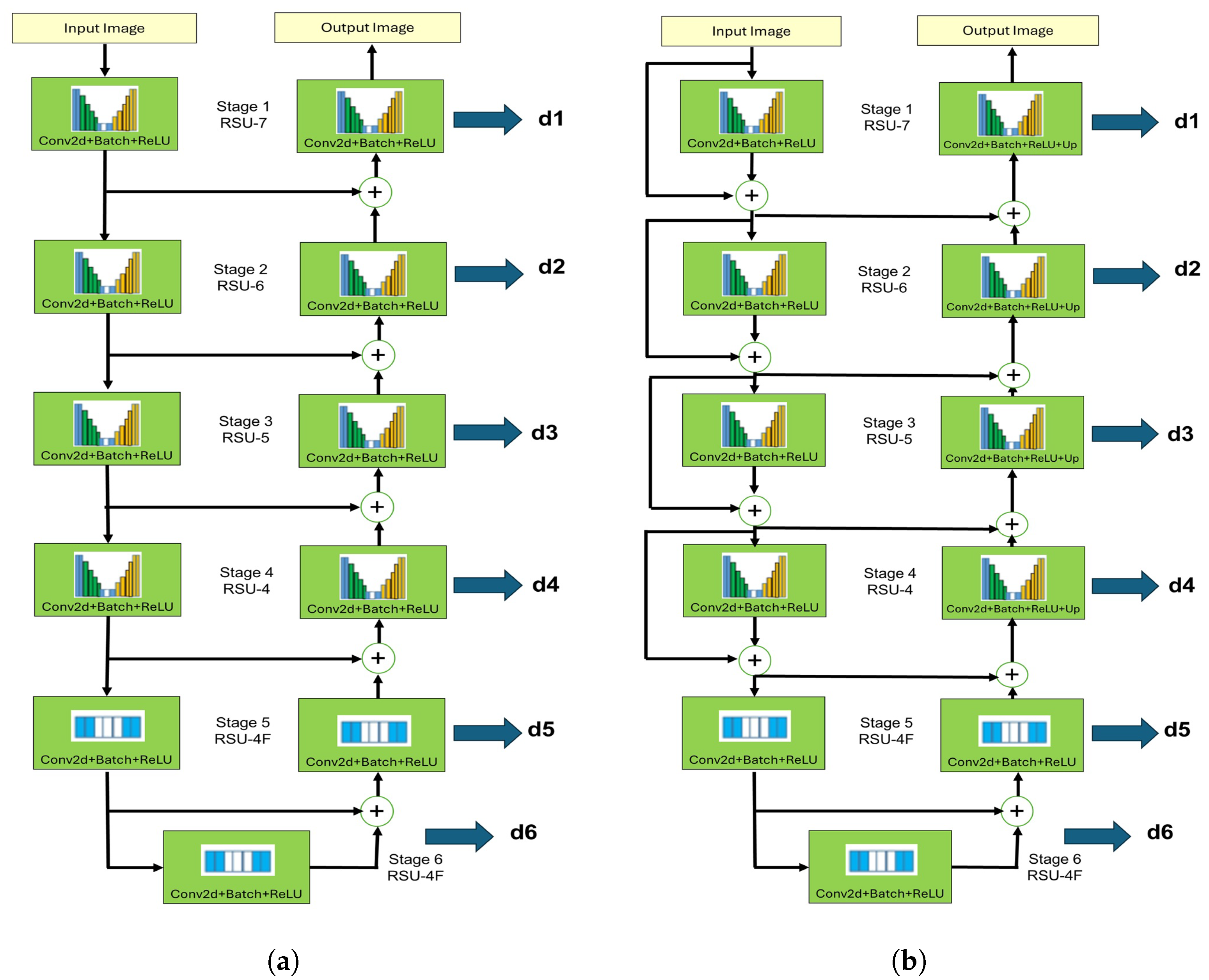
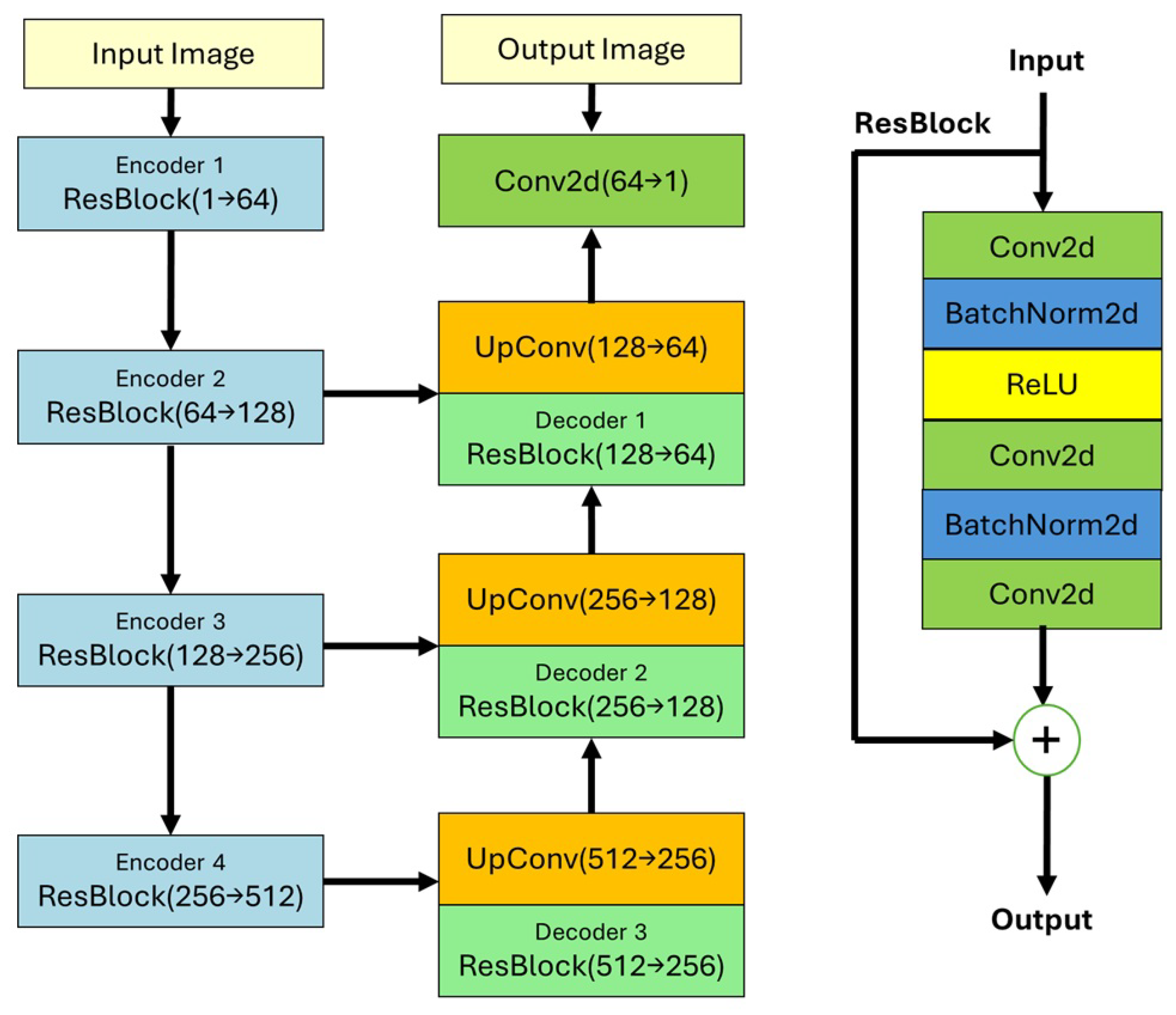
The outline of this article is as follows. Section 2 reviews previous work on image denoising, with an emphasis on PDE-based approaches. In Section 3, we introduce the specific nonlinear PDE formulations used in our framework. Section 4 describes the architecture of the general physics-informed denoising, while Section 5 details the neural network backbones used, and Section 6 discusses refinement through PINN denoising. The numerical benchmark results appear in Section 7 and conclude with key lessons and directions for future work in Section 8.

2. Related Work

2.1. Deep Learning Methods for Image Denoising

Deep learning methods can be classified into supervised [1], semi-supervised [49], and unsupervised learning approaches [50].

2.1.1. Supervised Learning

It relies on labeled data to guide the model in learning parameters for tasks such as image denoising [51]. For example, consider a denoising model defined as $y=x+ϵ$ where x, y, and $ϵ$ represent the clean image, noisy image, and additive Gaussian noise (AWGN) with a standard deviation of $\sigma$, respectively. Based on this model and Bayesian inference, learning the model parameters depends on a dataset of paired examples ${\left\{\left(x_k,y_k\right)\right\}}_{k=1}^N$, where $x_k$ and $y_k$ denote clean and noisy images k-th, and N is the total number of samples. The relationship can be expressed as $x_k=f\left(y_k,\theta ,m\right)$, where $\theta$ denotes the model parameters and m is the known noise level.

2.1.2. Unsupervised Learning

Does not require labeled data [52]. Instead, it identifies the underlying patterns within the input data to perform tasks such as domain transfer or image enhancement. For example, the Cycle-in-Cycle GAN (CinCGAN) [53] architecture performs super-resolution by first estimating a high-resolution label and then refining this estimate using loss functions and unlabeled data.

2.1.3. Semi-Supervised Learning

Combines labeled and unlabeled data [54]. It is particularly useful in scenarios with limited labeled samples, such as in medical diagnostics [55]. For example, the Semi-Supervised Learned Sinogram Restoration Network (SLSR-Net) [56] initially learns feature distributions from paired sinograms through a supervised component and then applies this knowledge in an unsupervised manner to reconstruct high-quality sinograms from unlabeled low-dose data [57].

2.2. CNNs for Image Denoising

Convolutional neural networks (CNNs) have demonstrated remarkable success in image processing tasks due to their flexible plug-and-play architectures [58]. LeNet [59], one of the first CNN models, used convolutional kernels of various sizes to effectively extract features for image classification. However, its reliance on the sigmoid activation function led to slow convergence, limiting its applicability in real-world scenarios [60]. The introduction of AlexNet marked a significant milestone in the field of deep learning. Its success stemmed from several key innovations: leveraging the computational power of GPUs, employing dropout to mitigate overfitting [61], using the ReLU activation function to accelerate stochastic gradient descent (SGD) [62], and incorporating data augmentation techniques. Despite its strong performance, the large convolutional kernels of AlexNet required significant memory [63], which restricted its use in resource-limited applications, such as smart cameras.

2.3. Recent Image Denoising Methods

Transformer-based denoisers, such as Swin Transformer/SwinIR-style models [64], use windowed self-attention to capture long-range dependencies and typically deliver strong PSNR/SSIM with fast, single-pass inference. In contrast, DIP-TV [45] (Deep Image Prior with Total Variation) is a training-free, per-image optimization approach that can work without clean datasets, but is slower and can over-smooth fine textures. Diffusion models (DDPMs) [65] provide powerful generative priors and often achieve excellent perceptual denoising, yet require iterative sampling with higher computational cost and potential hallucination if not constrained. DDRM [44] adapts diffusion priors to restoration by enforcing data consistency with an explicit degradation model, often improving fidelity over unconstrained diffusion, but still inherits multi-step inference and sensitivity to forward-model mismatch.

2.4. Recent Progress in PDE-Based Image Denoising

Recent work has progressed along three converging research directions (Table 2), with several studies emphasizing the implementation of PDE-based image denoising techniques.

i

New and generalized PDE formulations for denoising (including multiplicative/speckle noise): Variable- and fractional-order PDEs have been proposed to better adapt the smoothing strength to local structure and speckle statistics, improving detail preservation over classical anisotropic diffusion. Examples include a variable spatially exponent PDE for multiplicative noise [66] and fractional-order PDEs that enhance edge/texture fidelity while suppressing ultrasound noise [67]. Anisotropy-stabilized formulations continue to evolve, e.g., tunable despeckling guided by anisotropic diffusion within a degradation framework [68]. These works collectively report gains in PSNR/SSIM and texture retention compared to standard PM/TV baselines.

ii

Hybrid PINN/PDE–DL schemes that enforce physics during learning: PINN-style training that embeds PDE residuals and boundary conditions into loss has been shown to improve robustness and interpretability in imaging tasks. For image denoising and edge preservation, physics-informed blending of PDE priors has demonstrated improved artifact control over CNNs driven purely by data [69]. Beyond natural images, PINN denoisers have been specialized for modality-specific physics (e.g., high b-value diffusion MRI), showing superior fidelity under limited data [70]. Physics-informed microscopy reconstruction similarly integrates forward optics into a diffusion-conditioned architecture to suppress hallucinations [71].

iii

Generative diffusion models tailored to SAR despeckling with explicit noise physics have emerged as the state of the art. Regional DDPMs and diffusion posterior sampling strategies explicitly consider block-wise structure and speckle statistics to reduce texture loss and over-smoothing [72,73]. Conditional/efficient DDPMs further incorporate the SAR noise model and achieve strong quantitative and visual performance in synthetic and real scenes [74,75]. These methods consistently report gains in ENL/CNR while maintaining edges.

Table 2. Implementation case studies of PDE-based image denoising.

Method (PDE)	Noise Model	Dataset/Application	Ref.
Heat diffusion	Additive Gaussian	USC–SIPI, Kodak24; baseline smoothing	[76]
SRAD	Multiplicative speckle (Gamma)	Ultrasound, SAR	[77]
Nonlocal PDE/NL-TV	Multiplicative speckle	Gaussian test images; texture preservation	[78]
Complex diffusion	Additive Gaussian	Various natural images	[79]
Variance-stabilized PDE	Poisson	Microscopy images	[39]
Fourth-order PDE	Additive Gaussian	Various natural images	[80]
TV-Poisson (TV-KL)	Poisson	Various natural images	[81]
CED	Additive Gaussian	Fingerprint images	[82]

Table 2. Implementation case studies of PDE-based image denoising.

Method (PDE)	Noise Model	Dataset/Application	Ref.
Heat diffusion	Additive Gaussian	USC–SIPI, Kodak24; baseline smoothing	[76]
SRAD	Multiplicative speckle (Gamma)	Ultrasound, SAR	[77]
Nonlocal PDE/NL-TV	Multiplicative speckle	Gaussian test images; texture preservation	[78]
Complex diffusion	Additive Gaussian	Various natural images	[79]
Variance-stabilized PDE	Poisson	Microscopy images	[39]
Fourth-order PDE	Additive Gaussian	Various natural images	[80]
TV-Poisson (TV-KL)	Poisson	Various natural images	[81]
CED	Additive Gaussian	Fingerprint images	[82]

3. Denoising PDE Models

Partial differential equations (PDEs) are widely applied in various image processing tasks [42]. One powerful approach to solving PDEs using neural networks, particularly (FNNs) [83], is the physics-informed neural network framework (PINN) [69]. In a PINN, a neural network is designed to serve as a surrogate model for the PDE solution. Consider an FNN that takes inputs x and t, with hidden layers composed of $n_l$ neurons. The objective is to train the neural network to approximate the solution $u(x,t)$ using a function $f(x,t,\theta )$, where $\theta$ denotes the parameters of the network, including weight matrices and bias vectors. The output of the FNN is generated through an activation function, typically the hyperbolic tangent function tanh.

To enforce the PDE constraints, the PINN calculates the required k-th order derivatives of $f(x,t,\theta )$ regarding its inputs using automatic differentiation (AD) [84]. The backpropagation algorithm, an AD technique, is employed to calculate these derivatives within the neural network. AD consists of two main phases: a forward pass to compute variable values and a backward pass to compute their derivatives. The neural network is then restricted to satisfy the given PDE and its associated boundary and initial conditions. The training dataset $\tau$ includes two subsets of points: those sampled from the interior domain and those on the boundary. These points are collectively referred to as residual points. A loss function $L(\theta ,\tau )$ is defined as a weighted sum of $L_2-norms$ of the residuals of the PDE and the boundary conditions. This loss quantifies the deviation of the neural network from satisfying the problem constraints. The goal is to minimize $L(\theta ,\tau )$ to identify an optimal set of parameters $\theta$. Gradient-based optimization algorithms are used for this minimization. To achieve a high level of accuracy, it is essential to carefully tune various hyperparameters, including the network size, the number of residual points, and other model-specific settings.

These models form the mathematical backbone for traditional and modern image denoising techniques, including physics-informed neural networks (PINNs) that integrate such equations into their training process:

• Modified Perona–Malik Curvature Model (MPMC) Model: The MPMC model enhances classic Perona–Malik anisotropic diffusion by incorporating curvature information to better preserve edges during denoising. The Equation (1)  [30] is as follows:

  $${\displaystyle \frac{\mathsf{\partial }u}{\mathsf{\partial }t}}=\nabla ·\left(g\left(\left|k\right|\right)\nabla u\right)$$

  (1)

  where $u(x,y,t)$ is the image intensity, k is the curvature of the level lines, and $g(·)$ is an edge-stopping function that controls diffusion strength.
• Zhichang Guo (ZG) Model: A PDE model combining second- and fourth-order anisotropic diffusion was proposed to simultaneously smooth flat regions and preserve fine details. The Equation (2) [31] is as follows:

  $${\displaystyle \frac{\mathsf{\partial }u}{\mathsf{\partial }t}}={\lambda }_1\nabla ·(g_1\left(\left|\nabla u\right|\right)\nabla u)-{\lambda }_2{▵}^{2}u$$

  (2)

  where ${\lambda }_1,{\lambda }_2$ are regularization weights, $g_1(·)$ is an edge-preserving function, and ${▵}^{2}u$ is the biharmonic operator for fourth-order diffusion.
• Heat Equation Residual Model: The heat equation is the simplest form of isotropic diffusion used for image smoothing. The Equation (3) [85] is as follows:

  $${\displaystyle \frac{\mathsf{\partial }u}{\mathsf{\partial }t}}=▵u$$

  (3)

  This model blurs both noise and edges uniformly. The residual form is often used in deep learning to guide the network’s output $f(x,t,\theta )$ through a physics-informed loss Equation (4):

  $$R(x,t)={\displaystyle \frac{\mathsf{\partial }f}{\mathsf{\partial }t}}-▵f$$

  (4)
• General Diffusion Model: This model is a general formulation for anisotropic diffusion. The Equation (5) [44] is as follows:

  $${\displaystyle \frac{\mathsf{\partial }u}{\mathsf{\partial }t}}=\nabla ·\left(D(x,y,t)\nabla u\right)$$

  (5)

  where $D(x,y,t)$ is a diffusion tensor that controls the direction and strength of the smoothing, adaptable based on the characteristics of the image.

Speckle Model for Data Generation

Speckle noise in coherent imaging systems, such as SA,R is commonly modeled using a multiplicative noise model [86]:

$$Y=NX,$$

(6)

where $Y\in {\mathbb{R}}^{W\times H}$ is the noisy image observed (intensity domain), $X\in {\mathbb{R}}^{W\times H}$ is the underlying speckle-free image, and $N\in {\mathbb{R}}^{W\times H}$ is a positive random variable representing the speckle. For a multi-look SAR image with L independent looks, N follows a Gamma distribution with unit mean and variance $1/L$, whose probability density function (PDF) is

$$p\left(N\right)={\displaystyle \frac{L^L{N}^{L-1}{e}^{-LN}}{\Gamma \left(L\right)}},N\ge 0,L\ge 1,$$

(7)

where $\Gamma (·)$ is the Gamma function.

• Amplitude image: Many SAR processors work on the amplitude image, defined as the square root of the intensity: $x=\sqrt{X}$ for the clean image and $y=\sqrt{Y}$ for the observed one. The same multiplicative model applies:

  $$y=nx,$$

  (8)

  where n is the multiplicative speckle affecting the amplitude domain. In this case, n follows a Nakagami distribution with PDF:

  $$p\left(n\right)={\displaystyle \frac{2L^L{n}^{2L-1}{e}^{-L{n}^2}}{\Gamma \left(L\right)}},n\ge 0,L\ge 1.$$

  (9)
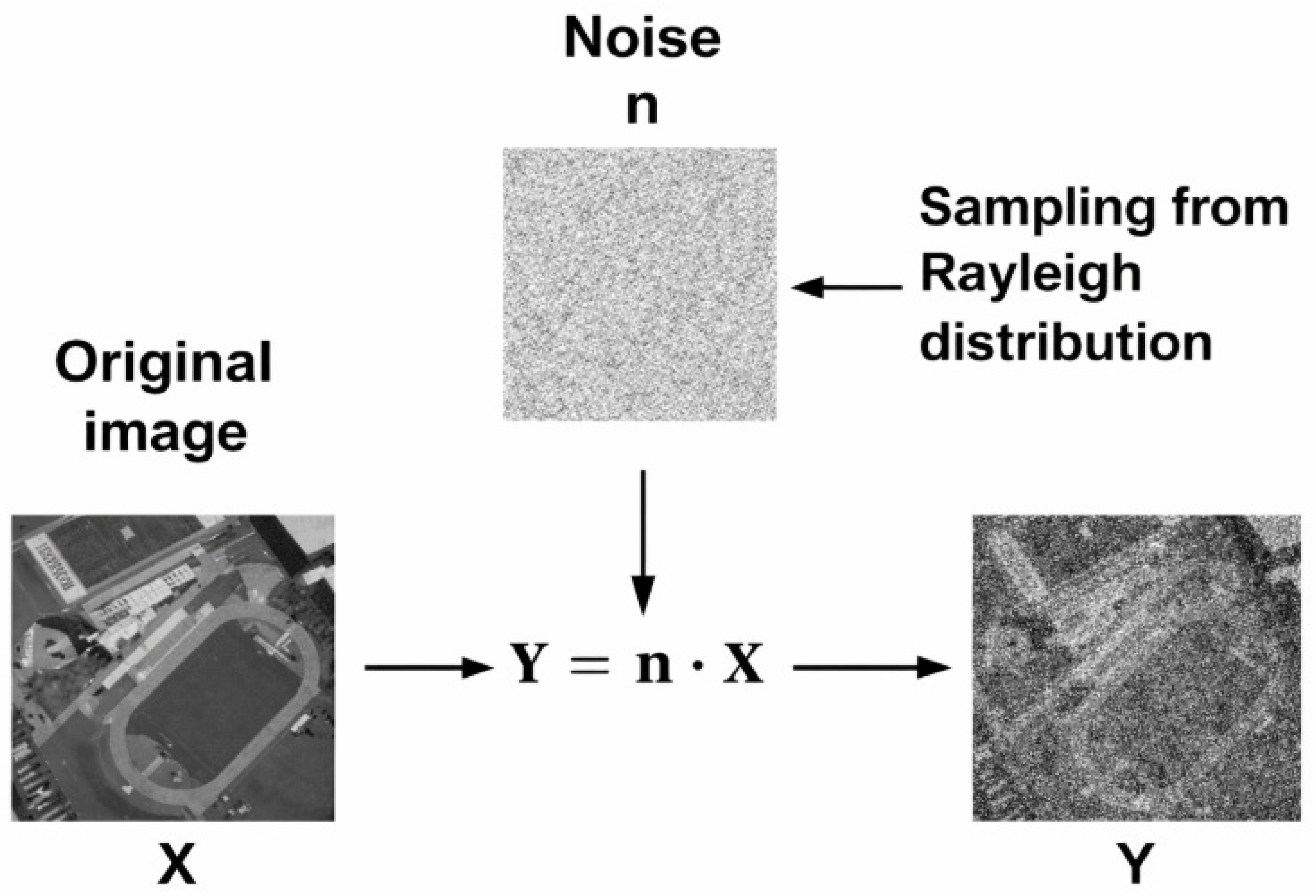
• Single-look image: A single-look ($L=1$) SAR image is obtained from one coherent measurement without multi-look averaging; it contains the strongest speckle fluctuations. For $L=1$, the Nakagami distribution in Equation (9) reduces to the Rayleigh distribution, which characterizes the amplitude speckle in single-look data (see Figure 1). This formulation allows us to synthesize speckle-corrupted images in either the intensity or the amplitude domain by drawing samples from the corresponding PDFs for any chosen number of looks L.

Image denoising is evaluated across additive levels of Gaussian white noise (AWGN) $\sigma \in \left\{15,25,50\right\}$, Poisson–Gaussian $\lambda \in \left\{1,4,8\right\}$, and speckle $\Gamma \in \left\{1,4,8\right\}$ in 8-bit images (range 0–255), following common practice. When images are normalized to $[0,1]$, the corresponding standard deviation, for example, by AWGN is $\widehat{\sigma }=\sigma /255$ and the variance is ${\widehat{\sigma }}^2={\left(\sigma /255\right)}^2$, which yields $\widehat{{\sigma }^2}\simeq \left\{1.20 \times {10}^{-5}, 9.60 \times {10}^{-5}, 3.84 \times {10}^{-4}\right\}$.

4. Proposed Framework

The present study proposes the framework illustrated in Figure 2, which integrates classical PDE priors into a deep neural network through a composite loss function. The network processes a noisy image, denoted as ${\widehat{X}}_N$, to produce a denoised output. Training is driven by Equation (10):

$$\begin{array}{c}\hfill L_{\mathrm{total}}=L_{\mathrm{PDE}}+{\lambda }_1{L}_{\mathrm{perceptual}}+{\lambda }_2{L}_{\mathrm{data}}+{\lambda }_3{L}_{\mathrm{IC}}+{\lambda }_4{L}_{\mathrm{BC}}\end{array}$$

(10)

The total loss ${\mathcal{L}}_{\mathrm{total}}$ used to train the physics-informed neural network (PINN) comprises multiple components, each designed to enforce the fidelity, physical consistency, and perceptual quality of the data. The weighting coefficients $\lambda$ are carefully tuned based on the validation performance to achieve an optimal balance between accurate data reconstruction and adherence to the underlying physical laws. Here, individual terms are defined as follows:

• PDE Loss: This term enforces that the prediction of the network $\widehat{X_r}$ satisfies the underlying residual of the PDE $\mathcal{N}\theta (·)$ by Equation (11). For each model, the derivatives in Equations (1)–(5) are obtained by automatic differentiation, ensuring exact gradients in terms of network parameters:

  $$L_{\mathrm{PDE}}={\left|\mathcal{N}\theta \left(\widehat{X_r}\right)\right|}_2^2$$

  (11)
• Perceptual Loss: The term “feature-space” ensures that the predicted image $\widehat{X_r}$ remains perceptually close to the original clean image $X_{ref}$ using the ${\mathcal{\ell }}_1$ norm by Equation (12). Let ${\varphi }_l(·)$ denote the activation in the layer l and $w_l$ its weight:

  $$L_{\mathrm{perc}}=\sum _{l\in \mathcal{S}}{w}_l{∥{\varphi }_l\left({\widehat{X}}_r\right)-{\varphi }_l\left(X_{\mathrm{ref}}\right)∥}_1.$$

  (12)
• Data Loss: This is a standard mean squared error term that compares the predicted and original images by Equation (13):

  $$L_{\mathrm{data}}={\left|\widehat{X_r}-X_{ref}\right|}_2^2$$

  (13)
• Initial Condition Loss: This term penalizes the deviation of the predicted field at $t=0$ from the known initial image $X_0$:

  $$L_{\mathrm{IC}}={\displaystyle \frac{1}{\left|\mathsf{\Omega }\right|}}\sum _{p\in \mathsf{\Omega }}{w}_{\mathrm{IC}}\left(p\right){∥{\widehat{X}}_r(p,0)-X_0\left(p\right)∥}_2^2,$$

  (14)

  where $w_{\mathrm{IC}}\left(p\right)\ge 0$ is an optional spatial weight or mask (e.g., to ignore unknown pixels). When the ground truth at $t=0$ is not available, we set $X_0$ to the observed input (or a priori).
• Boundary Condition Loss: We support standard BC types on $\mathsf{\partial }\mathsf{\Omega }$; n denotes the normal outward unit. Dirichlet BC (${\widehat{X}}_r=g$ on $\mathsf{\partial }\mathsf{\Omega }$):

  $$L_{\mathrm{BC}}={\displaystyle \frac{1}{\left|\mathsf{\partial }\mathsf{\Omega }\right|}}\sum _{q\in \mathsf{\partial }\mathsf{\Omega }}{w}_{\mathrm{BC}}\left(q\right){∥{\widehat{X}}_r(q,t)-g(q,t)∥}_2^2.$$

  (15)

5. Integrating PDE with Network DL Denoising

Four neural network architectures—UNet, ResUNet, U2Net, and ResU2Net—each integrated with the PDE formulation described in Section 3. All models were implemented in PyTorch and trained with the Adam optimizer using an early stopping criterion of loss $<{10}^{-4}$ or a maximum of 500 epochs.

• Case 1: A UNet-based architecture was used for PDE-guided image denoising (see Figure 3). The network was specifically adapted to accommodate multi-scale feature extraction, incorporating a symmetric structure composed of downsampling and upsampling paths. The architecture consisted of two main stages:

  1.

  Downsampling Path: The encoder utilized a sequence of convolutional layers followed by max-pooling operations to progressively reduce the spatial dimensions of the input noisy image ${\widehat{X}}_N$. The resolution of the feature map was sequentially downscaled through levels of 32, 64, 128, and 256 channels, allowing the abstraction of hierarchical features at multiple scales.

  2.

  Upsampling Path: The decoder used upsampling operations and convolutional layers to gradually restore the spatial resolution of the encoded features. Skip connections were integrated between the corresponding encoder and decoder layers to preserve fine-grained spatial details that are critical for accurate reconstruction.

  During training, the UNet was optimized not only to minimize the reconstruction error between the denoised output ${\widehat{X}}_R$ and the ground truth image ${\widehat{X}}_{ref}$, but also to satisfy a governing partial differential equation (PDE) model embedded within a composite loss function. Specifically, the total loss function combined three components: (i) a residual PDE loss enforcing physical consistency, (ii) an initial condition (IC) loss ensuring correct initialization behavior, and (iii) a boundary condition (BC) loss enforcing consistency along image borders. This physics-informed loss formulation guided the UNet to denoise in a manner aligned with the underlying diffusion dynamics, thereby improving generalization and preserving important structural features.
• Case 2: Residual U-Net (ResUNet) architecture was used to perform image denoising under partial differential equation (PDE) constraints (see Figure 4). The model takes as input a noisy image ${\widehat{X}}_N$ and outputs a denoised image ${\widehat{X}}_R$. The ResUNet structure incorporates deep residual learning into the classical encoder–decoder U-Net design to facilitate better gradient flow and capture complex features critical for PDE-driven restoration tasks. The architecture consists of the following main components:

  1.

  Encoder: The encoder progressively extracts hierarchical characteristics through a sequence of downsampling stages. Each stage consists of a ResidualBlock, which applies two convolutional layers (with Batch Normalization and ReLU activation) and a skip connection that directly adds the input to the output. The encoder maps the noisy input ${\widehat{X}}_N$ into a compact feature representation through the following encoder layer: enc1→ enc2 → enc3 → enc4.

  2.

  Decoder: The decoder reconstructs spatial resolution by successive upsampling operations (using transposed convolutions), followed by residual blocks. Skip connections are used between encoder and decoder layers to preserve spatial information lost during downsampling. Before concatenation, a cropping operation ensures that the dimensions of feature maps align with the decoder layer: dec3 ⟵ dec2 ⟵ dec1.

  3.

  Output Layer: A final 1 × 1 convolution maps the feature space to a single-channel image ${\widehat{X}}_R$, corresponding to the denoised reconstruction.

• Case 3: This case presents the U2Net architecture to perform image denoising under a physics-informed learning framework (see Figure 5a). The U2Net model, illustrated by the above class definition, processes a noisy image input ${\widehat{X}}_N$ and outputs a denoised prediction ${\widehat{X}}_R$, while leveraging a composite loss that includes PDE constraints. The U2Net is a deeply nested U-structure network composed of residual U-blocks (RSUs) at each stage. The model architecture can be summarized as follows:

  1.

  Encoder: The input noisy image ${\widehat{X}}_N$ is first passed through multiple encoding stages: stage1 ⟶ pool12 ⟶ stage2 ⟶ pool23 ⟶ stage3 ⟶ stage6.

  2.

  Decoder: After reaching the deepest feature representation ($hx6$), the network performs upsampling and decoding operations: stage5d ⟶ to ⟶ stage1d. Skip connections are implemented by concatenating encoder features with corresponding decoder layers, ensuring fine-grained spatial information is preserved.

  3.

  Side Outputs: Intermediate outputs (d1, d2, d3, d4, d5, d6) are generated at different resolutions through 1 × 1 convolutional layers, which are later fused to form the final denoised prediction d0.

  4.

  Final Prediction: The final denoised image ${\widehat{X}}_R$ is obtained by applying a sigmoid activation function to the fused side outputs: ${\widehat{X}}_R=\sigma \left(d0\right)$.

• Case 4: ResU2Net model, a lightweight variant of the U2Net architecture, was adapted to incorporate PDE priors for physics-informed noise removal (see Figure 5b). The network takes as input a noisy image ${\widehat{X}}_N$ and produces a denoised output ${\widehat{X}}_R$. The architecture is composed of multiple residual U-shaped (RSU) blocks, each designed to effectively capture multi-scale spatial features while maintaining computational efficiency:

  1.

  Encoder: The noisy image ${\widehat{X}}_N$ is successively processed through six RSU stages (Stage 1 to Stage 6), where each stage refines the spatial representations using residual encoding. As shown in the schematic, each RSU block comprises a Conv2D+BatchNorm+ReLU stack, which applies downsampling to enlarge the receptive field while reducing spatial resolution.

  2.

  Decoder: After the final encoder stage (Stage 6), the model reconstructs high-resolution features via a mirrored decoder structure. Each decoder stage (from Stage 5 to Stage 1) receives upsampled features concatenated with skip connections from its corresponding encoder stage, followed by residual RSU decoding blocks to recover spatial details. This design enables efficient feature reuse and context fusion.

  3.

  Residual Connections: As highlighted in the image, skip connections and element-wise summation between encoder and decoder outputs enhance feature propagation and support robust gradient flow during training.

  4.

  Side Outputs and Deep Supervision: The architecture includes six intermediate side outputs (denoted as d1 through d6), each extracted from a corresponding decoder stage. These outputs undergo upsampling and contribute to deep supervision, encouraging multi-scale feature learning.

  5.

  Final Reconstruction: All side outputs are fused through a final convolutional layer (outconv) to generate the denoised output image ${\widehat{X}}_R$.

6. Progressive Refinement via Physics-Informed Neural Network Denoising

Figure 6 illustrates the progressive improvement in image quality over iterations of the PINN-based denoising process [26]. Starting from the original and noisy inputs (top row), the bottom sequence shows how the model gradually reconstructs structural details while suppressing speckle noise. Early iterations retain high levels of noise and artifacts, whereas later stages achieve clearer and sharper restorations that closely resemble the ground truth. This highlights the capacity of the physics-informed approach to balance noise reduction with feature preservation throughout the training process.

PINN-Based Image Denoising: Pseudocode

The proposed algorithm (see Algorithm 1) performs image denoising (see Figure 7) based on PINN by integrating a neural network backbone, such as UNet or ResUNet, with a residual based on diffusion-based partial differential equations (PDE), following principles similar to those described in [44]. First, the chosen model is constructed with symmetric encoder–decoder stages (with skip connections or residual blocks). During training, each noisy input Y is passed through the network to produce a prediction $\widehat{u}$:

1.

Data fidelity loss $L_{\mathrm{data}}$ (mean squared error between $\widehat{u}$ and the clean image X).

2.

PDE loss $L_{\mathrm{PDE}}$ enforcement $\kappa \Delta \widehat{u}-\mathrm{model}\left(\widehat{u}\right)\approx 0$.

3.

Perceptual loss $L_{\mathrm{perc}}$ (L₁ distance).

4.

Boundary Condition Loss $L_{\mathrm{BC}}$→$\mathrm{MSE}(\widehat{u},0)$.

5.

Loss of initial condition $L_{\mathrm{IC}}$→$\mathrm{MSE}(\widehat{X_{r0}},X_0)$.

The total loss is a weighted sum of these terms and is minimized via the Adam optimizer over a fixed number of epochs. Periodic logging of individual loss components ensures stable convergence. The final output is the denoised image $\widehat{X}=\mathrm{model}\left(Y\right)$, which effectively suppresses the speckle while preserving structural details.

Algorithm 1 Physics-informed PINN–PDE image denoising scheme

Require: Clean image X, noisy image Y, number of epochs E, architecture $arch$ Ensure: Denoised image $\widehat{X}$  Model construction   1: function BuildModel($arch$)   2:     if $arch=$ “UNet” then   3:         Define encoder–decoder with standard UNet blocks   4:     else if $arch=$ “ResUNet” then   5:         Define encoder–decoder with residual UNet blocks   6:     else if $arch=$ “U2Net” then   7:         Define encoder–decoder with nested U2 blocks   8:     else if $arch=$ “ResU2Net” then   9:         Define encoder–decoder with residual U2 blocks (ResU2Net–ZG backbone) 10:     end if 11:     return ${\mathrm{model}}_{\theta }$ 12: end function PDE residual 13: function DiffusionResidual(u, ${\mathrm{model}}_{\theta }$, $\kappa$) 14:     Compute discrete Laplacian $\Delta u$ using a fixed convolution kernel 15:     ${\widehat{f}}_{\theta }\left(u\right)\leftarrow {\mathrm{model}}_{\theta }\left(u\right)$ 16:     return $r\left(u\right)=\kappa \Delta u-{\widehat{f}}_{\theta }\left(u\right)$ 17: end function Loss function 18: function ComputeLoss($\widehat{u}$, X, ${\mathrm{model}}_{\theta }$) 19:     $L_{\mathrm{data}}\leftarrow \mathrm{MSE}(\widehat{u},X)$ 20:     $L_{\mathrm{IC}}\leftarrow \mathrm{MSE}(X_r,X_0)$               ▹ Initial-condition consistency 21:     $L_{\mathrm{BC}}\leftarrow \mathrm{MSE}({\widehat{u}}_{|\mathsf{\partial }\mathsf{\Omega }},0)$                   ▹ Boundary condition 22:     $L_{\mathrm{PDE}}\leftarrow \mathrm{MSE}(\mathrm{DiffusionResidual}(\widehat{u},{\mathrm{model}}_{\theta },\kappa ),0)$ 23:     $L_{\mathrm{perc}}\leftarrow {\mathrm{L}}_1(\widehat{u},X)$ 24:     $L_{\mathrm{total}}\leftarrow L_{\mathrm{data}}+L_{\mathrm{PDE}}+0.1L_{\mathrm{perc}}+0.03L_{\mathrm{IC}}+0.02L_{\mathrm{BC}}$ 25:     return $L_{\mathrm{total}}$ 26: end function Training loop 27: function TrainPINN($X,Y,E,arch$) 28:     ${\mathrm{model}}_{\theta }\leftarrow$BuildModel($arch$) 29:     Initialize the Adam optimizer for parameters $\theta$ 30:     for $e=1$ to E do 31:         $\widehat{u}\leftarrow {\mathrm{model}}_{\theta }\left(Y\right)$ 32:         Resize/crop $\widehat{u}$ to match the spatial size of X 33:         $L\leftarrow$ComputeLoss($\widehat{u},X,{\mathrm{model}}_{\theta }$) 34:         Update $\theta$ with one Adam step using ${\nabla }_{\theta }L$ 35:         if $emod100=0$ then 36:            Log e, L, $L_{\mathrm{PDE}}$ and $L_{\mathrm{perc}}$ 37:         end if 38:     end for 39:     return ${\mathrm{model}}_{\theta }\left(Y\right)$ 40: end function Main procedure 41: Load X and generate Y (e.g., $Y\leftarrow \mathrm{add}\_\mathrm{speckle}\left(X\right)$) 42: $\widehat{X}\leftarrow$TrainPINN($X,Y,500,$ “ResU2Net”) 43: Display and/or save $\widehat{X}$

7. Experimental Results

The performance of the proposed PINN–PDE denoising framework was evaluated using a dedicated protocol (see

Table 3. PDE-based deep learning denoising on $256\times 256$ image inputs using different backbone architectures and GPU platforms.

Model	GeForce RTX 3060	Jetson Nano	Jetson Xavier
UNet	Real-time (20–30 FPS)	Slow (1–3 FPS)	Moderate (8–12 FPS)
ResUNet	Fast (15–20 FPS)	Slow (0.5–2 FPS)	Moderate (6–10 FPS)
U2Net	Moderate (10–15 FPS)	Very slow ($<1$ FPS)	Slow (4–7 FPS)
ResU2Net	Moderate (8–12 FPS)	Not feasible without quantization	Slow (3–6 FPS)

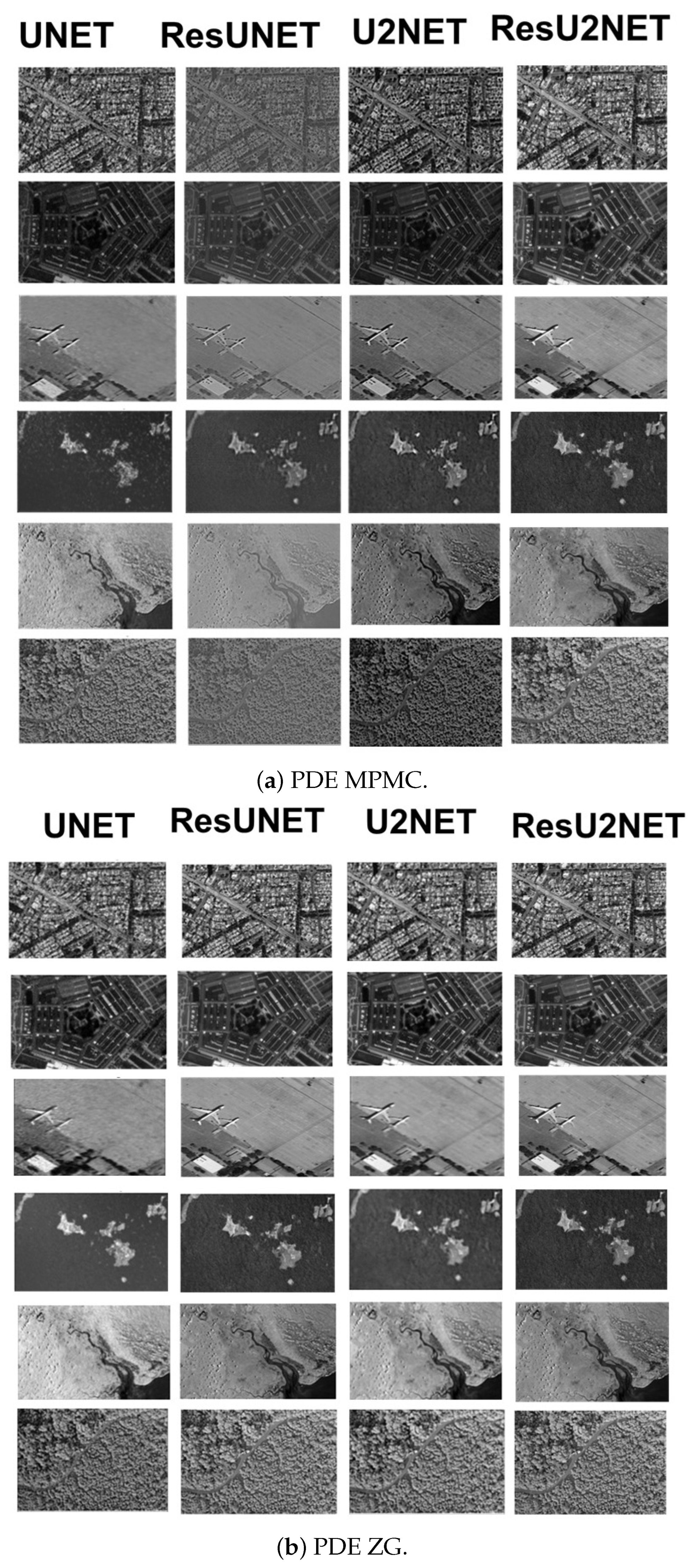
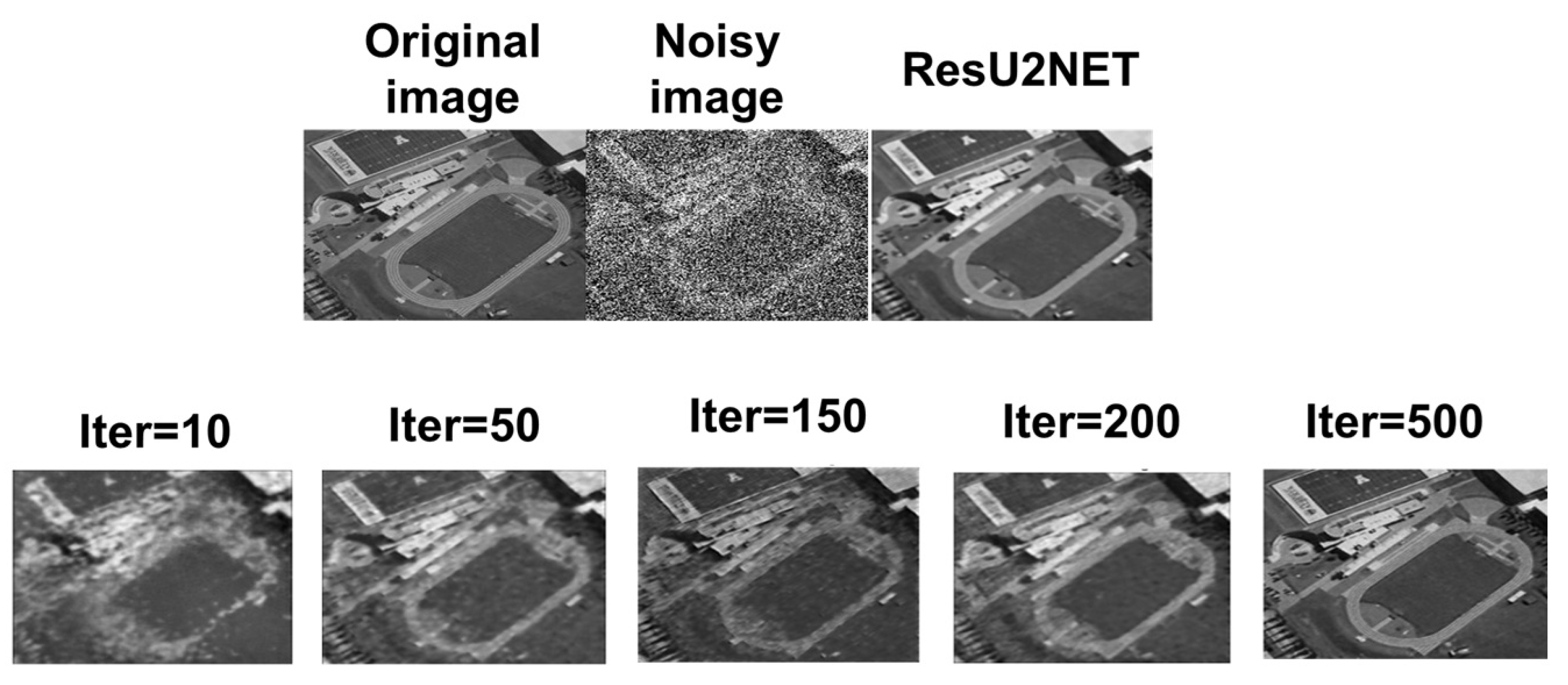
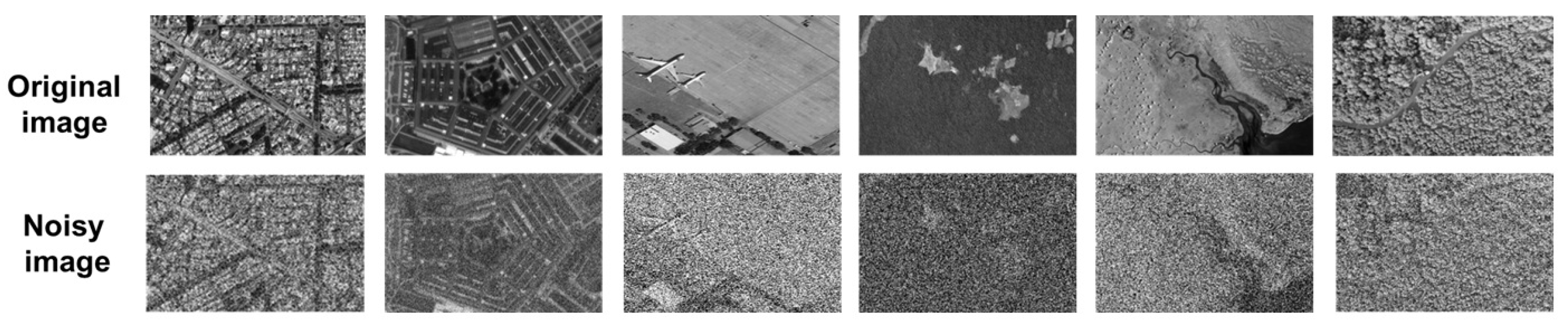
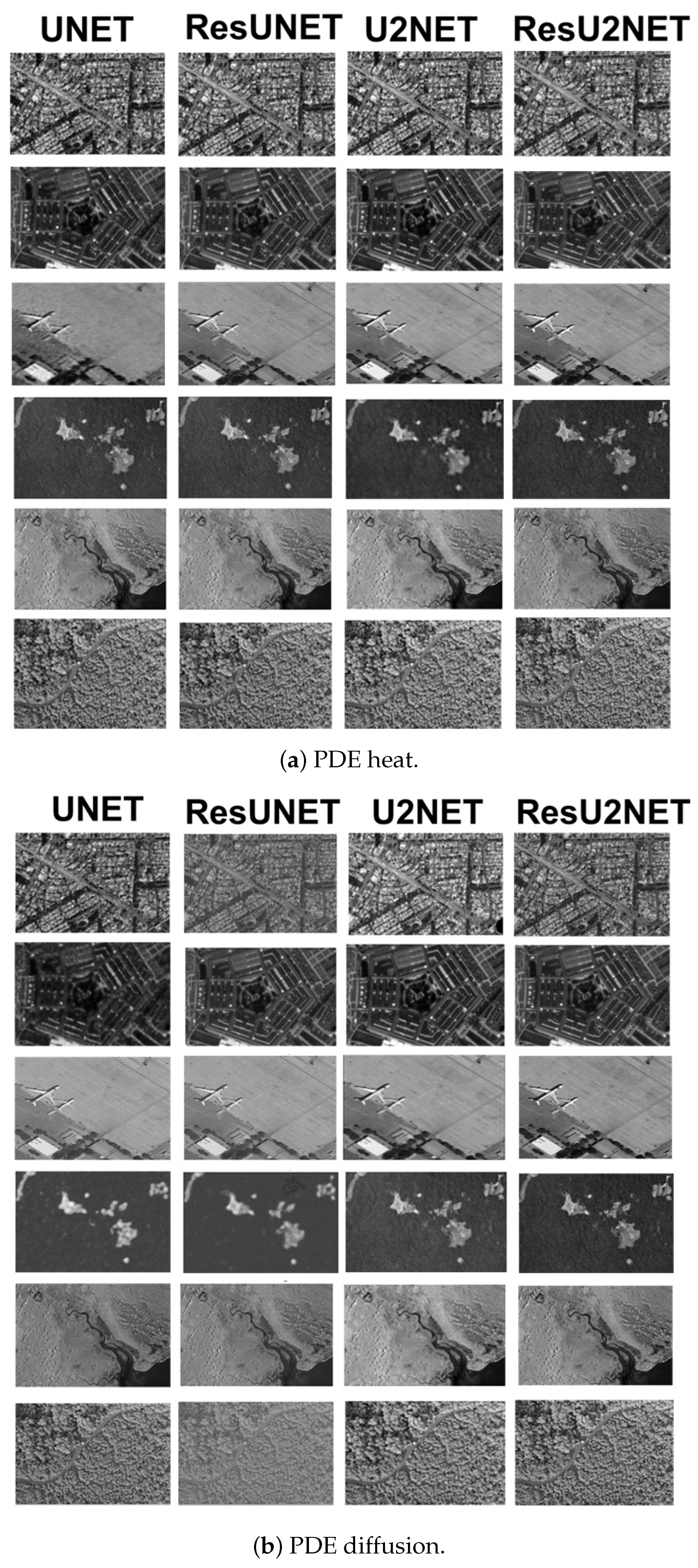
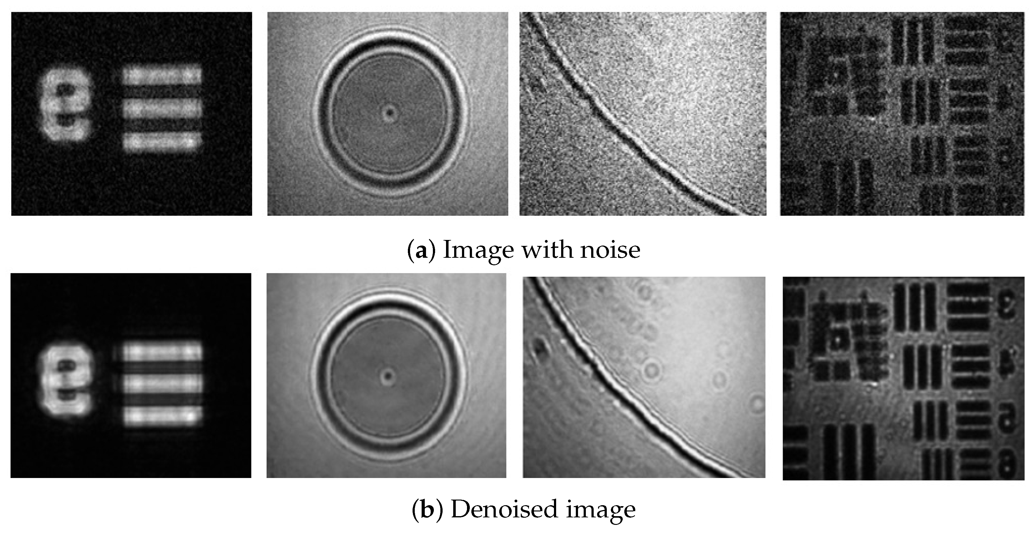
). Specifically, we applied the system to aerial scene images from the RESISC and AID datasets [87,88]. To simulate noise (see Figure 8 and Figure 9) and testing in the laboratory (see Figure 10), we used the widely accepted multiplicative noise model defined as $Y=N·X$, where $Y\in {\mathbb{R}}^{W\times H}$ denotes the observed noisy image, $X\in {\mathbb{R}}^{W\times H}$ is the underlying clean image, and $N\in {\mathbb{R}}^{W\times H}$ represents the speckle component modeled using a Nakagami–Rayleigh distribution [86]. The enhanced (denoised) images were subsequently assessed using the neural network architecture described in Section 5. Methods were evaluated and compared using PSNR, SSIM, ENL, and CNR to validate the PINN approach across multiple neural network configurations (see

Table 4. PSNR (dB) ↑ and SSIM ↑ scores for denoised images obtained with the heat, diffusion, MPMC, and ZG PDE models.

Method	Heat (PSNR/SSIM)	Diffusion (PSNR/SSIM)	MPMC (PSNR/SSIM)	ZG (PSNR/SSIM)
UNet	15.01/0.75	16.63/0.78	17.25/0.75	20.95/0.77
ResUNet	27.13/0.78	20.03/0.88	15.72/0.89	29.90/0.87
U2Net	26.70/0.79	25.69/0.90	16.44/0.93	30.82/0.89
ResU2Net	32.24/0.89	34.72/0.91	37.24/0.97	42.24/0.98

and

Table 5. ENL ↑ and CNR ↑ scores for denoised images obtained with the heat, diffusion, MPMC, and ZG PDE models. Higher values indicate better speckle suppression and contrast preservation.

Method	Heat (ENL/CNR)	Diffusion (ENL/CNR)	MPMC (ENL/CNR)	ZG (ENL/CNR)
UNet	8.01/2.55	10.00/2.12	8.30/2.25	9.69/4.36
ResUNet	9.10/6.06	9.58/3.41	10.24/6.46	11.21/4.53
U2Net	9.11/5.55	10.47/4.31	16.76/6.96	11.72/7.36
ResU2Net	9.61/6.43	11.60/4.46	18.58/8.30	22.24/9.61

). PSNR quantifies the fidelity of the reconstruction in decibels (higher values are better; values >20 dB typically indicate acceptable quality). SSIM measures the perceptual similarity of luminance, contrast, and structure (higher is better; values >0.5 denote moderate to strong similarity). For speckle, the equivalent number of looks (ENL) gauges residual multiplicative noise within homogeneous regions (higher ENL indicates stronger speckle suppression). Finally, CNR assesses edge/target visibility relative to background noise (higher CNR is better suited for contrast and boundary preservation). Reporting all four metrics—PSNR/SSIM for fidelity, and ENL/CNR for speckle-specific behavior—provides a balanced basis for comparison with previous work [89,90].

7.1. Correctness and Reliability Analysis

Given a noisy input image y, our network produces a reconstruction $\widehat{x}=f_{\theta }\left(y\right)$ by minimizing a composite training objective:

$${\mathcal{L}}_{\mathrm{total}}\left(\theta \right)={\lambda }_{\mathrm{PDE}}{\mathcal{L}}_{\mathrm{PDE}}\left(\widehat{x}\right)+{\lambda }_1{\mathcal{L}}_{\mathrm{per}}\left(\widehat{x}\right)+{\lambda }_2{\mathcal{L}}_{\mathrm{data}}(\widehat{x},x_{\mathrm{ref}})+{\lambda }_3{\mathcal{L}}_{\mathrm{IC}}\left(\widehat{x}\right)+{\lambda }_4{\mathcal{L}}_{\mathrm{BC}}\left(\widehat{x}\right),$$

(16)

where the PDE loss enforces numerical consistency with the selected prior through a discrete residual operator $\mathcal{R}(·)$:

$${\mathcal{L}}_{\mathrm{PDE}}\left(\widehat{x}\right)={\displaystyle \frac{1}{\left|\mathsf{\Omega }\right|}}\sum _{p\in \mathsf{\Omega }}{∥\mathcal{R}\left(\widehat{x}\right)\left(p\right)∥}_2^2.$$

(17)

For the linear priors (heat/diffusion), $\mathcal{R}$ is a local, bounded finite-difference operator; hence ${\mathcal{L}}_{\mathrm{PDE}}$ acts as a structured Tikhonov-like regularizer that stabilizes the mapping $y\mapsto \widehat{x}$ by discouraging high-frequency components inconsistent with the PDE prior. For nonlinear priors (MPMC/ZG), $\mathcal{R}$ remains local and curvature-/edge-aware, providing a physically meaningful constraint that suppresses noise while preserving geometry. Although the overall optimization is non-convex due to $f_{\theta }$, the PDE residual term improves reliability by shrinking the feasible set toward PDE-consistent reconstructions, reducing sensitivity to spurious solutions.

7.2. Repeatability Across Images and Noise Levels

Table 6. PSNR (dB) achieved by competing image denoising methods on standard test images based on the ResU2Net–ZG method.

Method	C.Man	House	Peppers	Starfish	Monar	Airpl	Parrot	Boat	Man	Couple	Average
$\mathit{\sigma }=\mathbf{15}$
BM3D [18]	31.92	34.94	32.70	31.15	31.86	31.08	31.38	32.14	31.93	32.11	32.38
WNNM [91]	32.18	35.15	32.97	31.83	32.72	31.40	31.61	32.28	32.12	32.18	32.70
EPLL [92]	31.82	34.14	32.58	31.08	32.03	31.16	31.40	31.91	31.97	31.90	32.10
TNRD [93]	32.19	34.55	33.03	31.76	32.57	31.47	31.63	32.15	32.24	32.11	32.51
DnCNN-S [94]	32.62	35.00	33.29	32.23	33.10	31.70	31.84	32.42	32.47	32.47	32.87
MemNet [95]	32.51	35.10	33.31	32.12	33.04	31.53	31.73	32.43	32.45	32.49	32.83
Ours	38.27	43.53	38.33	41.40	42.22	42.50	41.39	41.06	41.53	41.68	41.19
$\mathit{\sigma }=\mathbf{25}$
BM3D	29.45	32.86	30.16	28.56	29.25	28.43	28.93	29.91	29.62	29.72	29.98
WNNM	29.64	33.23	30.40	29.03	29.85	29.69	29.12	30.03	29.77	29.82	30.26
EPLL	29.24	32.04	30.07	28.43	29.30	28.56	28.91	29.29	29.63	29.48	29.63
TNRD	29.71	32.54	30.55	29.02	29.86	28.98	29.18	29.92	29.88	29.71	30.66
DnCNN-S	30.19	33.09	30.85	29.40	30.23	29.13	29.42	30.22	30.11	30.12	30.43
MemNet	30.02	33.25	30.87	29.35	30.24	29.03	29.30	30.21	30.08	30.14	30.41
Ours	37.90	42.99	35.57	39.80	41.84	40.40	37.47	38.72	41.02	40.13	39.58
$\mathit{\sigma }=\mathbf{50}$
BM3D	26.13	29.69	26.68	25.04	25.82	25.10	25.90	26.78	26.81	26.46	26.73
WNNM	26.42	30.33	26.91	25.43	26.32	25.42	26.09	26.97	26.94	26.64	27.04
EPLL	26.02	28.76	26.63	25.04	25.78	25.24	25.84	26.65	26.72	26.24	26.35
TNRD	26.62	29.48	27.10	25.42	26.31	25.59	26.16	26.94	26.98	26.50	26.81
DnCNN-S	27.00	30.02	27.29	25.70	26.77	26.46	26.88	27.19	27.24	26.90	27.14
MemNet	27.24	30.70	27.51	25.76	27.19	26.96	26.50	27.06	27.24	27.14	27.40
Ours	35.88	41.19	28.53	35.57	37.86	35.73	33.93	35.60	30.97	31.16	34.64

reports the PSNR standard test images under three Gaussian noise levels ($\sigma \in \{15,25,50\}$). A key reliability property is consistent dominance: our method attains the highest PSNR for every image and every noise level, indicating that performance is not driven by a small subset of favorable cases.

To quantify the effect size, we compare against the strongest deep baseline in Table 6 on a per-image basis and report the mean improvement with a $95\%$ confidence interval (CI) over the 10 images:

$$\begin{array}{cc}\hfill \sigma =15:& \Delta \mathrm{PSNR}=8.48\mathrm{dB}[7.21,9.74];\hfill \end{array}$$

(18)

$$\begin{array}{cc}\hfill \sigma =25:& \Delta \mathrm{PSNR}=9.33\mathrm{dB}[7.89,10.78];\hfill \end{array}$$

(19)

$$\begin{array}{cc}\hfill \sigma =50:& \Delta \mathrm{PSNR}=7.50\mathrm{dB}[5.09,9.90].\hfill \end{array}$$

(20)

Moreover, the improvement holds for images at each noise level, yielding a sign-test probability of $p=2^{-10}\approx 9.77\times {10}^{-4}$ per noise level, which supports the notion that the gain is systematic rather than incidental. At the aggregate level (Average column in Table 6), our PSNR is also substantially higher: $41.19$ vs. $32.87$ dB ($\sigma =15$), $39.58$ vs. $30.43$ dB ($\sigma =25$), and $34.64$ vs. $27.14$ dB ($\sigma =50$), confirming a large accuracy margin under increasingly severe corruption.

7.3. Discussions

The simulation Figure 9 of the results demonstrates the effectiveness of the proposed PINN–PDE-based denoising framework in improving image quality and suppressing speckle noise across a variety of neural network backbones and PDE models. In Table 4, the PSNR and SSIM metrics consistently improve when any of the heat, diffusion, MPMC, or ZG PDE models are applied. Among these, the ZG model yields the highest overall gains in both metrics across all architectures. For example, ResU2Net achieves the best performance, reaching a PSNR of 42.24 dB and an SSIM of 0.98, indicating highly effective noise removal while preserving structural image details. The observed performance trend, heat < diffusion < MPMC < ZG, suggests that progressively more sophisticated PDE formulations provide stronger regularization and structural fidelity in the denoising process.

Similarly, Table 5 shows clear improvements in ENL and CNR, which are critical for evaluating speckle suppression and contrast preservation. Again, the ZG model stands out, with ResU2Net achieving the highest scores. ENL = 22.24 and CNR = 9.61 dB, indicating excellent homogeneity in flat regions and strong contrast between regions of interest. Notably, the MPMC and diffusion models also show competitive results, outperforming simpler models like heat, particularly in terms of CNR.

Compared with traditional methods (see Table 6 and

Table 7. Numerical evaluations on image denoising and speckle suppression. The proposed ResU2Net–ZG method consistently outperforms competing approaches.

Method	PSNR (dB) ↑	SSIM ↑	Model
SAR-DRN [96]	27.93	0.81	UNet with TV regularization.
RSIDNet [97]	31.84	0.94	CNN-based encoder–attention–decoder architecture.
DnCNN [94]	31.90	0.93	Feed-forward denoising convolutional neural network.
ECNDNet [98]	31.60	0.93	Convolutional neural denoising network.
ADNet [99]	34.14	0.96	Attention-guided denoising convolutional neural network.
WNNM [91]	31.90	0.85	Weighted nuclear norm minimization.
$TV\text{-}{L}^2$ [100]	30.28	0.89	Nonlinear PDE-based total variation model ($L^2$ fidelity).
$TV\text{-}{H}^{-1}$ [100]	31.53	0.89	Nonlinear PDE-based total variation model ($H^{-1}$ fidelity).
Pureformer [43]	29.64	0.86	Transformer-based Image Denoising.
Diffusion Models [101]	31.64	—	Denoising Diffusion Models with Iteratively Preconditioned Guidance.
Self-argumented(ViT) [102]	25.53	0.75	Noise2Noise Image Denoising.
Deep Image Prior [103]	33.10	0.961	Deep Image Prior for image denoising.
Ours	42.24	0.98	PINN–ResU2Net (physics-informed ResU2Net with ZG prior).

) such as models based on BM3D, EPLL, TNRD, MEmNet, SAR-DRN, WNNM, and PDE, our proposed methods show moderate performance, with PSNR values below 32 dB and SSIM scores ranging from 0.81 to 0.89. Deep learning-based models such as DnCNN, ECNDNet, and RSIDNet achieve better results, with PSNR around 31.6–31.9 dB and SSIM up to 0.94. In particular, ADNet, an attention-guided CNN, achieves the best among these with 34.14 dB PSNR and 0.96 SSIM. However, the proposed PINN-ResU2Net model significantly outperforms all others, achieving a PSNR of 42.24 dB and an SSIM of 0.98, demonstrating the effectiveness of combining physics-informed neural networks with the ResU2Net architecture for high-quality image denoising.

Although the proposed PINN–PDE-based denoising framework demonstrates state-of-the-art performance in PSNR, SSIM, ENL, and CNR, several limitations remain. The current evaluation relies mainly on simulated and benchmark datasets, which may not fully reflect the variability and complexity of real-world noise patterns. Joint optimization of PDE residuals and network parameters also introduces additional computational cost, particularly for large-scale or high-resolution images. Moreover, the framework currently employs a fixed set of PDE models (heat, diffusion, MPMC, and ZG), which may limit its adaptability to different noise characteristics. Future work will focus on extending the framework to real-world and multimodal datasets, enhancing computational efficiency through model compression and hardware acceleration, and incorporating adaptive PDE selection strategies. Integration of uncertainty estimation into the PINN formulation is also planned to improve the interpretability and reliability of the model.

The proposed model achieves strong accuracy in speckle-degraded images (see

Table 8. Overview comparison between modern image denoising techniques and the proposed ResU2Net–ZG model.

Method	PSNR/SSIM	Pros	Cons
Transformer denoisers [104]	51.16/0.99	High reconstruction quality on natural images.	Increased memory footprint and computational cost.
Diffusion models [101]	32.40/—	Flexible modeling of complex noise distributions.	High training and sampling complexity.
Self-supervised/ unsupervised [105]	32.46/0.81	Do not require clean target images for training.	Typically trail supervised state-of-the-art performance.
Deep unrolling [106]	30.19/0.80	Strong generalization linked to iterative optimization priors.	Requires careful tuning and model-specific design.
GAN-based denoisers [107]	32.87/—	Good perceptual quality and sharper textures.	Training and stabilization are more difficult.
Wavelet-domain deep learning [108]	28.55/—	Good detail recovery in the transform domain.	May be less flexible across diverse noise types.
Speckle-specific self-supervised [109]	30.61/0.88	Preserves structural information in speckle-dominated images.	Performance can be sensitive to acquisition conditions.
Ours (ResU2Net–ZG)	42.24/0.98	Robust denoising when labeled data are scarce; physics-informed prior.	More complex loss design and higher computational cost.

), outperforming classical and several modern baselines in our setting while remaining interpretable through its PDE priors. Compared with transformer denoisers and diffusion models, it is lighter and more data-efficient; although those methods can reach higher peaks on natural images at a greater memory/compute cost. Unlike self-supervised/SAR-specific approaches, our supervised, physics-guided design preserves structures more reliably when clean supervision is available and generalizes well across backbones; however, it introduces extra loss terms and training overhead. Deep-unrolling and plug-and-play frameworks offer strong generalization but incur iterative inference; GAN variants enhance perceptual sharpness, yet risk hallucinations; wavelet-domain nets are efficient but less flexible. In general, our method strikes a practical balance of quality, robustness, and interpretability for speckle denoising, with the main trade-off being the additional computation of physics-informed losses.

The results in

Table 9. Quantitative comparison of denoising performance of ResU2Net–ZG across multiple datasets and noise models (AWGM and Poisson–Gaussian).

Dataset	AWGM			Poisson–Gaussian
	$\mathit{\sigma }=\mathbf{15}$	$\mathit{\sigma }=\mathbf{25}$	$\mathit{\sigma }=\mathbf{50}$	$\mathit{\lambda }=\mathbf{1}$	$\mathit{\lambda }=\mathbf{4}$	$\mathit{\lambda }=\mathbf{8}$
AID [88]	33.00/0.90	38.20/0.96	39.49/0.98	38.26/0.96	40.23/0.98	40.60/0.98
BSD68 [110]	36.81/0.97	29.54/0.88	28.45/0.84	38.77/0.98	37.70/0.97	37.47/0.97
Urban100 [111]	40.69/0.97	39.23/0.96	28.04/0.87	39.43/0.97	39.26/0.96	38.64/0.96
DIV2K [112]	40.37/0.97	39.17/0.97	38.72/0.97	41.68/0.98	40.00/0.97	39.20/0.96
Kodak24 [113]	39.41/0.96	39.15/0.96	33.69/0.87	38.61/0.96	39.69/0.97	40.93/0.97
Set12 [1]	33.48/0.92	33.50/0.91	36.88/0.95	36.96/0.96	37.11/0.95	38.02/0.96
RESISC [87]	40.65/0.97	36.58/0.92	33.24/0.86	41.27/0.98	40.16/0.97	40.48/0.97

and

Table 10. Quantitative comparison of denoising performance of ResU2Net–ZG across multiple datasets for speckle noise.

Dataset	Speckle
	$\Gamma =\mathbf{1}$	$\Gamma =\mathbf{4}$	$\Gamma =\mathbf{8}$
AID [88]	40.18/0.97	38.94/0.97	38.64/0.96
BSD68 [110]	39.86/0.98	38.53/0.97	36.12/0.97
Urban100 [111]	39.57/0.98	38.79/0.95	38.03/0.95
DIV2K [112]	41.90/0.97	40.19/0.97	39.79/0.96
Kodak24 [113]	38.65/0.95	39.07/0.96	39.29/0.96
Set12 [1]	37.37/0.96	38.33/0.96	38.49/0.96
RESISC [87]	40.79/0.98	40.16/0.96	37.37/0.95

demonstrate the scalability and versatility of the proposed denoising framework across a wide range of datasets with different image characteristics and under varying noise conditions. Consistently high PSNR and SSIM values across all noise levels indicate robust generalization, particularly for challenging scenarios such as high variability AWGN ($\sigma =50$) and strong multiplicative noise ($\Gamma =8$). Performance remains stable across both natural and remote sensing datasets, highlighting the adaptability of the method to varying image domains and noise distributions.

8. Conclusions and Future Work

This study presented a physics-informed denoising framework that integrates four partial differential equation (PDE) priors: heat, diffusion, MPMC, and ZG—into deep neural network architectures to address image denoising and speckle suppression. Theoretically, the work establishes a bridge between classical PDE-based modeling and modern deep learning, enhancing interpretability and improving noise suppression by embedding physical priors into the learning process. Practically, the proposed framework demonstrates strong reconstruction performance, achieving high PSNR, SSIM, ENL, and CNR values on the RESISC and AID aerial datasets, with the ZG prior in combination with ResU2Net providing the most consistent results. This confirms the effectiveness of the PINN–PDE approach in restoring speckle-degraded imagery across different backbones of the network.

The main contributions of this research are threefold. First, it introduces a unified PINN–PDE denoising strategy that is generalizable across architectures. Second, it provides a systematic comparison of the PDE priors, identifying the ZG model as particularly effective. Third, it validates the framework for challenging aerial imagery, achieving state-of-the-art results in multiple quality metrics. These contributions highlight the value of incorporating physics-based constraints into deep learning for robust image restoration. In practical terms, the framework offers several advantages. By leveraging PDE priors, it reduces dependence on large labeled datasets, making it suitable for real-world applications where ground truth is limited. Its modular structure enables easy integration with existing neural models, and the enhanced preservation of structural details makes it well-suited for downstream tasks such as classification, object detection, and change analysis. Moreover, the use of interpretable PDE dynamics increases trust and traceability, which are critical in sensitive domains such as environmental monitoring and medical imaging.

The experiments rely mainly on simulated and benchmark datasets, which may not fully capture the complexity of real-world noise. Joint optimization of PDE residuals and network parameters increases computational costs, particularly for high-resolution images. Furthermore, the use of fixed PDE priors constrains the adaptability of the framework to complex or mixed noise types. Future research will address these challenges by developing adaptive PDE learning strategies that dynamically tune the priors during training and incorporate attention mechanisms and multi-scale representations to better preserve edges and fine structures. We will also extend the framework to realistic noise and acquisition conditions through systematic stress tests, including saturation/clipping augmentation with censored-loss training, EMI-like artifact modeling (stripe/impulse/burst corruption), and misregistration robustness via controlled shifts/warps and joint alignment–denoising. Finally, we will optimize the method for efficient, low-power deployment (FPGA/embedded-GPU), enabling integration into operational imaging pipelines and edge devices, thereby increasing its practical impact.