Article

Field-Measurement-Based Wideband Modeling and System-Level Simulation of MMC-HVDC Converter Stations for High-Frequency Disturbance Studies


1
Electric Power Research Institute, State Grid Zhejiang Electric Power Co., Ltd., Hangzhou 310014, China
2
State Key Laboratory of Electrical Insulation and Power Equipment, Xi’an Jiaotong University, Xi’an 710049, China
3
Construction Branch, State Grid Zhejiang Electric Power Co., Ltd., Hangzhou 310014, China
4
State Grid Zhejiang Electric Power Co., Ltd., Hangzhou 310014, China
*
Author to whom correspondence should be addressed.
Electronics 2026, 15(17), 3860; https://doi.org/10.3390/electronics15173860
Submission received: 13 June 2026 / Revised: 14 August 2026 / Accepted: 25 August 2026 / Published: 27 August 2026

Abstract

This study establishes a field-measurement-based wideband modeling and station-level simulation framework for conducted high-frequency (HF) disturbance studies in modular multilevel converter-based high-voltage direct-current (MMC-HVDC) stations. Full-scale engineering-site frequency-response measurements are used to identify kHz-to-MHz terminal models of the arm reactor and the valve-side winding of the converter transformer. The arm reactor is fitted in the admittance domain by vector fitting and synthesized as a passive parallel network containing the main inductive path and multiple damped resistor–inductor–capacitor (RLC) branches. The transformer valve-side winding is represented by a Foster I/II hybrid π -type terminal network reconstructed from two single-phase port-impedance measurements. The validated equipment models are integrated into a representative Power Systems Computer-Aided Design (PSCAD) station model. A 2 ms valve-side source sequence, constructed from nearest-level-control switching instants and a parameterized switching-transient template, is applied in paired injection and zero-injection simulations. For the representative event, the source peak is 605.6 V. Over the first 4 μ s, the arm-reactor terminal reaches 972.6 V, while the direct-current (DC)-side, valve-side alternating-current (AC), and point-of-common-coupling (PCC) responses reach 534.2, 438.4, and 151.9 V, respectively. The corresponding peak changes relative to the source are + 4.11 , 1.09 , 2.81 , and 12.01 dB. The DC-side response contains a dominant damped oscillation near 0.61 MHz, and the AC/PCC transfer varies markedly across 0.2–2.0 MHz. In a separate control-identical comparison over the first 2.5 μ s, the field-identified and lumped models give DC-side peaks of 171.9 and 1.23 V and PCC peaks of 121.4 and 3.93 V under the same excitation. The framework connects field-identified equipment terminal behavior with station-level time-domain propagation analysis and provides a modeling basis for broadband resonance screening and conducted electromagnetic-interference (EMI) assessment.

1. Introduction

Flexible high-voltage direct-current (HVDC) transmission increasingly relies on the modular multilevel converter (MMC), a topology introduced for a wide power range [1] and now used in renewable integration and long-distance power transfer [2]. In an MMC-HVDC station, repeated insulated-gate bipolar transistor (IGBT) turn-on and turn-off transients and submodule switching inject conducted high-frequency (HF) disturbances into the main circuit [3,4]. Their source characteristics, propagation paths, modeling methods, and suppression measures have been reviewed systematically [5]. Once injected, the disturbance travels through the arm reactors, converter transformers, direct-current (DC)- and alternating-current (AC)-side equipment, and the external network. Its station-level response depends on both the source waveform and the kHz-to-MHz terminal characteristics of the primary equipment. Conducted electromagnetic-interference (EMI) analysis and broadband resonance screening thus require station models that retain the measured wideband behavior of key equipment.
Conventional station models are designed mainly for fundamental-frequency operation, control studies, and slow electromagnetic-transient (EMT) studies. They normally represent the arm reactor with a lumped inductance and the converter transformer with a low-frequency T- or Γ -type circuit, omitting the multiple resonances, capacitive paths, and phase transitions that appear in the kHz-to-MHz range. Such omissions can alter the frequency-dependent voltage division and obscure the station nodes at which a disturbance is enhanced. Detailed MMC-HVDC EMI studies show that the converter valve, arm reactor, transformer, and external network jointly form the conducted propagation path [5,6]. Transformer capacitances affect HF propagation and MMC-station resonance [7,8], while winding- and capacitance-based resonance models confirm that the HF terminal response cannot be reduced to leakage inductance alone [9,10]. Parasitic capacitance likewise governs the HF response and first resonance of inductive equipment [11,12]. These findings motivate field-derived wideband terminal models embedded in the station circuit.
Three research routes are most relevant. Impedance-based small-signal models characterize converter–network resonance and stability around an operating point [13,14,15,16]; their frequency-domain formulation is not intended to reproduce the time-domain propagation of individual switching transients. Frequency-response-based equipment models reproduce transformer terminal behavior in electromagnetic-transient studies [17,18]. Vector fitting, stable pole relocation, and passivity enforcement provide the rational-model basis [19,20,21,22]. Measurement-based implementations include commercial sweep frequency-response analysis (sFRA) modeling of a distribution transformer, a 45-MVA transformer model obtained from a 5 Hz–10 MHz sweep, synthesis from driving-point admittance, and field identification of a converter transformer [8,23,24,25]. These studies show that measured terminal models can be extended to full-scale equipment and embedded in EMT programs, although equipment representation or a specific resonance condition remains the central focus. Wideband EMT models follow a third route. Zhu et al. combined device dynamics with extracted package, submodule, and valve-tower parasitics in a station model [6], while parasitic-parameter circuits have also reproduced high-frequency oscillations during MMC-HVDC DC faults [26].
Table 1 compares representative studies by system or object, model basis, main focus, and evidence or scale.
The comparison separates adjacent modeling tasks. Models developed for control analysis use small-signal formulations to identify stability mechanisms associated with converter and network interactions. Machine fault EMT models embed internal generator states, converter topology studies develop new power conversion structures, and equipment models derived from measurements retain terminal resonances. The present study extends the measurement-based equipment modeling route to station-level EMT analysis. Passive terminal networks are derived from field measurements of a full-scale arm reactor and converter transformer and used to quantify the propagation paths of switching disturbances. Among the compared studies, the complete chain from field measurement to equipment modeling and station-level propagation analysis remains unaddressed.
This paper addresses this gap by identifying wideband equivalent models of key MMC-HVDC primary equipment from field frequency-response measurements and coupling them with a representative station-level Power Systems Computer-Aided Design (PSCAD) model. A valve-side switching excitation demonstrates the measurement-to-model-to-station workflow. The framework is not tied to this waveform; other measured or synthesized HF sources can be applied to the same platform to examine propagation paths and resonance risks. The main contributions are as follows:
  • A field-measurement-driven wideband modeling workflow is established for full-scale engineering-site primary equipment. It combines admittance-domain vector fitting and passive parallel-branch synthesis for the arm reactor with a Foster I/II hybrid π -type terminal model for the valve-side winding of the converter transformer, thereby reducing reliance on design-only parasitic parameters or reduced-scale prototypes.
  • The field-identified terminal models are integrated into a representative PSCAD station-level MMC-HVDC platform while the converter switching, modulation, control, and external network are retained. This bridges equipment-level frequency-response identification and station-level time-domain conducted-HF analysis.
  • A paired injection–baseline simulation procedure isolates the source-driven station response. The representative event quantifies the time-domain peak change and frequency-selective propagation toward the arm-reactor, DC-side, valve-side AC, and point-of-common-coupling (PCC) terminals, and identifies a dominant DC-side oscillation near 0.61 MHz. A four-run control-identical comparison with conventional lumped equipment models further quantifies how the terminal representation changes the predicted path response.
The remainder of the paper is organized as follows. Section 2 develops the wideband models; Section 3 describes the field measurements, model verification and PSCAD implementation; Section 4 reports the representative propagation case; and Section 5 concludes.

2. Wideband Modeling of Key Equipment

2.1. Vector-Fitting-Based Wideband Model of the Arm Reactor

The arm reactor is a single two-terminal device whose port impedance spans several decades over the band of interest—inductive and almost zero at low frequency, but reaching the order of 10 5 Ω at high-frequency resonance peaks. Direct rational fitting of the impedance Z ( f ) is ill-conditioned because the algorithm tends to sacrifice low-frequency accuracy in order to fit the large high-frequency resonance peaks. To avoid this, the model is built in the admittance domain.

2.1.1. Rational Approximation

Let Z meas ( f ) = | Z ( f ) | e j φ ( f ) denote the field-measured impedance. The corresponding admittance is
Y meas ( f ) = 1 / Z meas ( f ) .
Here, f is expressed in Hz , j is the imaginary unit, | Z ( f ) | and Z meas are expressed in Ω , φ is expressed in rad , and Y meas is expressed in S . Vector fitting (VF) approximates Y meas by a stable rational form
Y ( s ) n = 1 N c n s p n + d + s e ,
where s = j 2 π f , { p n } C are the poles (real or in complex-conjugate pairs), { c n } are the residues, and d and e are the asymptotic terms. The set C denotes the open left half-plane. The complex-frequency variable s and each pole p n have units of s 1 ; each residue c n has units of S s 1 , while d and e have units of S and F , respectively. The rational order N is dimensionless. The poles are first relocated using the Sanathanan–Koerner iteration [30]. This pole-relocation idea forms the basis of vector fitting for rational approximation of frequency-domain responses [20], and later refinements improve the pole-relocating properties of the algorithm [21]. The residues and asymptotic terms are then solved by weighted least-squares with weights w i = 1 / | Y meas ( f i ) | . The index i identifies a measured sample at f i ( Hz ), and w i has units of Ω so that the weighted admittance residual is dimensionless. Candidate rational orders from N = 4 to N = 20 are evaluated in increments of two. The selection considers full-band approximation error, pole stability and the complexity of the synthesized circuit; the numerical results are reported in Section 3.3.

2.1.2. Synthesis to a Fully Parallel Equivalent Network

Once ( p n , c n , d , e ) have been identified, each rational term is mapped to a physically interpretable parallel branch following the rational-approximation structure of vector fitting [20]:
  • A real pole p n with residue c n contributes an RL series branch with
    L = 1 Re ( c n ) , R = Re ( p n ) Re ( c n ) .
  • A complex-conjugate pole pair ( p n , p n * ) with residues ( c n , c n * ) contributes a parallel resistor–inductor–capacitor (RLC) resonant branch with
    L = 1 2 Re ( c n ) , R = 2 | Re ( p n ) | L ,
    C = 1 [ Re 2 ( p n ) + Im 2 ( p n ) ] L , f 0 = 1 2 π L C .
  • The constant asymptotic term d contributes a parallel conductance G p = Re ( d ) , or equivalently a shunt resistance R p = 1 / G p . The proportional asymptotic term e, when retained in the final fit, contributes a static shunt capacitance C p = Re ( e ) .
In Equations (3)–(5), Re ( · ) and Im ( · ) denote the real and imaginary parts, and | · | denotes magnitude. These relations follow by matching a real-pole term or a complex-conjugate pole pair to the admittance of the corresponding physical branch. The units of R, L, C, and f 0 are Ω , H , F , and Hz , respectively. A physical-plausibility screening is applied to remove spurious branches (e.g., ones whose R and L are simultaneously below physically meaningful thresholds for an arm reactor at this voltage class), and a single global damping resistor R damp is added in parallel to control the quality factor of the dominant resonance. Each retained branch is a physical R L C branch with non-negative R, L and C, and the global damping resistor ( R damp = 200 k Ω ) is a positive shunt resistance whose value is chosen so that the synthesized parallel anti-resonance peak reproduces the measured peak magnitude (of the order of 2 × 10 5 Ω ). The synthesized network is passive by construction because it is a parallel interconnection of passive one-ports and a purely dissipative shunt resistance; the branch-removal and damping steps only add loss or discard non-physical terms and hence cannot violate passivity. In the implemented arm-reactor model, no separate static C p branch is retained; the capacitive behavior is represented by the fitted resonant branches, while the retained shunt branch is resistive. The resulting network captures, in physically interpretable branches: (i) the main inductive path that dominates low-frequency energy transfer; (ii) the high-frequency capacitive and resonant behavior associated with inter-turn, inter-layer and to-ground parasitics [12]; and (iii) additional damped branches associated with skin/proximity effects and local geometric resonances.

2.1.3. Parameter Identification Procedure

The candidate-order sweep gives full-band average relative admittance errors of 7.28 dB at N = 4 , 27.19 dB at N = 18 and 28.72 dB at N = 20 . The N = 20 rational approximation is retained after confirming that all 20 fitted poles have negative real parts, following improved VF pole-relocation practice [21]. The selected rational admittance is screened for physical branch parameters during circuit synthesis, consistent with passivity requirements for rational admittance models [22]. Conjugate-pole pairing, physical branch screening and the positive damping branch produce the ten-branch passive network shown in Figure 1 and listed in Table 2. The rational fitting order and implemented branch count are reported separately because circuit synthesis does not map each fitted pole to an independent PSCAD branch. For the present dataset, N = 20 is treated as an engineering accuracy–complexity choice within the evaluated range.

2.2. Foster I/II Hybrid π -Network Model

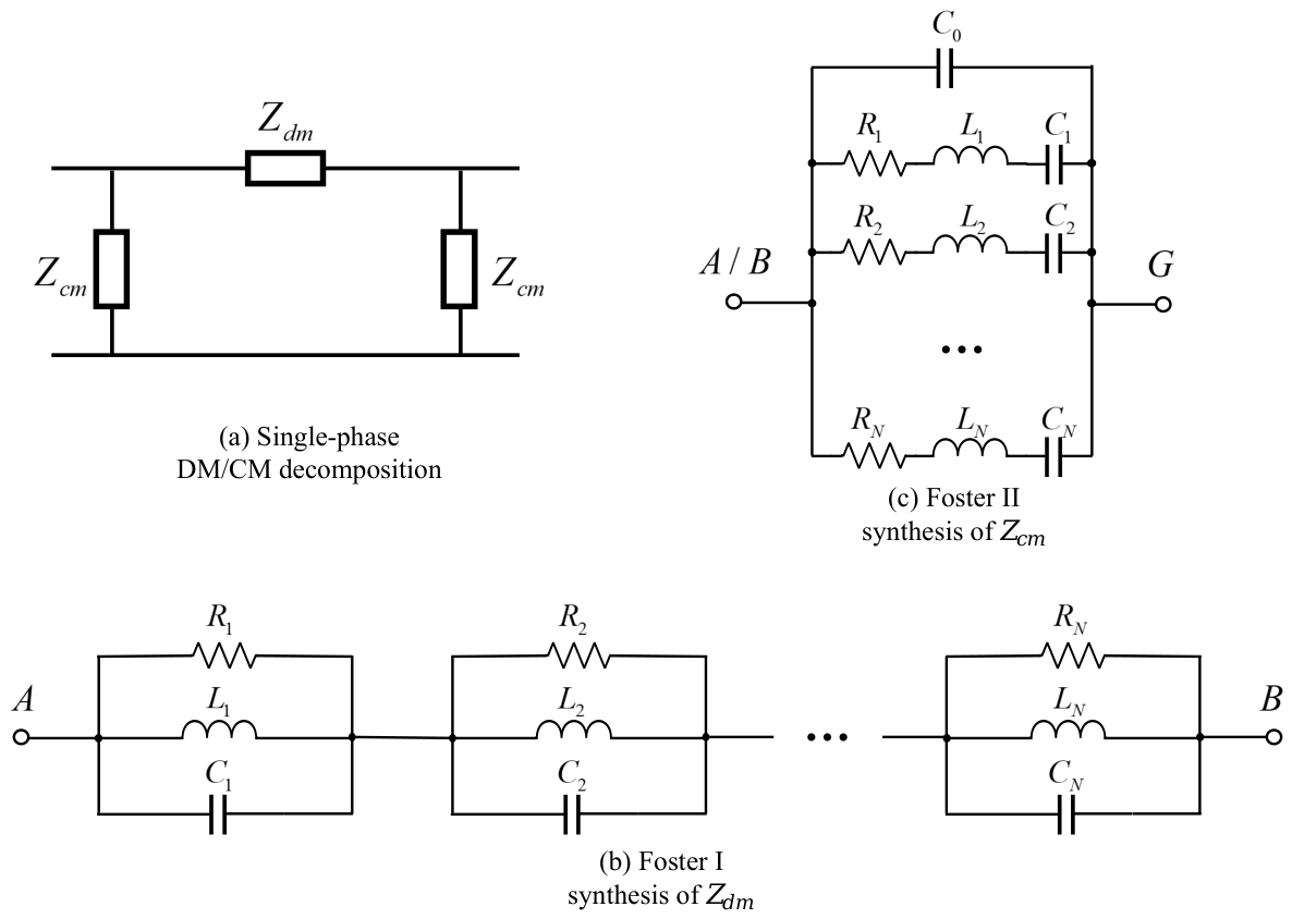
In this work, the wideband terminal model of the single-phase converter transformer is established for its valve-side winding, because this is the winding directly exposed to the valve-side switching disturbance. The grid-side winding and the valve-to-grid magnetic coupling are retained through the standard two-winding transformer model in the system-level simulation; only the valve-side winding is augmented by the wideband terminal equivalent developed here. The two terminals of the valve-side winding are denoted A and B, and the transformer tank (reference ground) is denoted G. In the frequency band considered here, the valve-side terminal behavior is decomposed into a differential-mode (DM) impedance Z dm between A and B—the terminal-to-terminal impedance of the valve-side winding—and two common-mode (CM) impedances Z cm from A and B to G, which represent the winding-to-tank paths. Such terminal-path representation is consistent with high-frequency transformer modeling for transient studies [17]. Gustavsen’s wideband transformer modeling further supports the use of measured terminal responses as the basis for transformer high-frequency representation [18]. Measured transformer network functions have also been used with vector fitting to characterize broadband transformer behavior [19]. The resulting single-phase π -type equivalent network consists of a series branch Z dm between A and B and two shunt branches Z cm connected from A and B to the reference ground, the two shunt branches being taken as identical. Under this definition, Z cm denotes the impedance of one shunt branch, whereas the terminal short-circuit measurement gives the parallel equivalent of the two shunt branches.

2.2.1. DM/CM Impedance Reconstruction

Two single-phase port-impedance measurements are used to reconstruct the CM and DM components. The measured quantities z 1 and z 2 , and the reconstructed quantities Z cm and Z dm , are expressed in Ω ; their common frequency argument f is expressed in Hz .
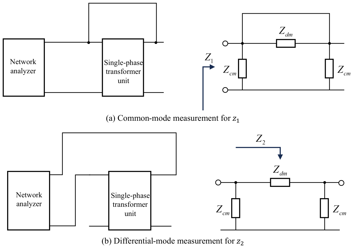
  • CM measurement: Terminals A and B are short-circuited, and the impedance between the short-circuited terminal and the reference ground G is measured as z 1 ( f ) . Since the two ends of Z dm are at the same potential, the DM branch is bypassed and the two Z cm branches are in parallel, giving
    z 1 ( f ) = Z cm ( f ) 2 , Z cm ( f ) = 2 z 1 ( f ) .
  • DM measurement: The impedance between terminals A and B is measured directly as z 2 ( f ) . From the port AB, the measured impedance consists of the direct DM branch Z dm in parallel with the ground-return path formed by the two CM branches in series; i.e.,
    z 2 ( f ) = Z dm ( f ) 2 Z cm ( f ) = 2 Z cm ( f ) Z dm ( f ) 2 Z cm ( f ) + Z dm ( f ) .
After Z cm ( f ) is obtained from (6), the DM impedance is calculated from (7) as
Z dm ( f ) = 2 Z cm ( f ) z 2 ( f ) 2 Z cm ( f ) z 2 ( f ) .
The factor of two in Equation (6) results from the two identical CM shunt paths connected in parallel during the CM measurement. Equation (7) combines the direct DM path with the series connection of the two CM paths, and solving that parallel relation for Z dm gives Equation (8). Thus, the field-derived sequences { Z cm ( f ) } and { Z dm ( f ) } are obtained for subsequent Foster-network parameter identification. The reconstruction in (8) becomes ill-conditioned when z 2 2 Z cm , i.e., when the DM branch barely loads the port; over the measured band the denominator 2 Z cm z 2 stays well above the measurement noise floor, so the reconstructed Z dm remains stable.

2.2.2. Foster I-Type Network for the DM Impedance

The DM frequency response is inductive at low frequency (dominated by the total leakage inductance L eq ) and exhibits multiple parallel resonance peaks at higher frequencies. A Foster I-type network represents this behavior using N p parallel R L C tanks connected in series:
Z dm ( s ) = k = 1 N p 1 R k + 1 s L k + s C k 1 .
Here, N p is the dimensionless number of differential-mode branches. The units of R k , L k , and C k are Ω , H , and F , respectively, and Z dm is expressed in Ω . At very low frequency, the capacitor of each tank is open and the resistor is shorted by the inductor; the total impedance reduces to k s L k , which is anchored to the measured total leakage inductance. Each tank is initialized by partitioning the magnitude curve at its resonant peaks, applying the textbook resonance relations
f k = 1 2 π L k C k , | Z dm ( f k ) | = R k ,
Here, f k is the kth resonance frequency in Hz , and | Z dm ( f k ) | and R k are expressed in Ω . One off-resonance reference point per region provides the third equation used to determine R k , L k , and C k analytically.

2.2.3. Foster II-Type Network for the CM Impedance

The CM frequency response is capacitive at low frequency (dominated by the total winding-to-ground stray capacitance C 0 ) and exhibits multiple series resonance valleys at higher frequencies. It is represented in this work by a Foster II-type network with a static shunt capacitance C 0 in parallel with N s series R L C branches:
Y cm ( s ) = s C 0 + k = 1 N s 1 R k + s L k + 1 s C k .
Here, Y cm is expressed in S , C 0 is expressed in F , and N s is the dimensionless number of common-mode branches. The units of R k , L k , and C k are Ω , H , and F , respectively. Because terminals A and B are equipotential in the CM measurement, the sweep voltage is applied between the shorted winding terminals and the transformer tank; no terminal-to-terminal winding voltage is intentionally imposed. The resulting Y cm characterizes the winding-to-tank displacement-current paths and their associated resonances. The Foster II network in Equation (11) is a linear time-invariant terminal equivalent identified for this measured HF path. The retained two-winding transformer provides the fundamental-frequency voltage transformation and magnetic coupling, while the Foster II network supplies the measured kHz-to-MHz CM terminal behavior. This layered representation follows wideband transformer modeling practice in which frequency-sweep terminal response and low-frequency magnetic behavior are represented by separate model components [31]. C 0 is initialised from the slope of the low-frequency segment in the log–log plane, and each series branch is initialised at a resonance valley in the same way as (10), with the peak replaced by the local minimum.

2.2.4. Parameter Identification Procedure

The DM and CM model parameters are obtained by first reconstructing Z dm ( f ) and Z cm ( f ) from the two single-phase field measurements, and then identifying the resonance peaks or valleys used to initialize the Foster branches. If necessary, the branch parameters are slightly adjusted within physically meaningful ranges so that the calculated magnitude and phase responses follow the measured frequency-response curves. The overall valve-side-winding wideband terminal model, comprising the DM/CM decomposition and the Foster I/II syntheses, is summarized in Figure 2. The numerical parameters and fitting accuracy for the studied transformer are reported in Section 3.3.

3. Field Measurement and System-Level Implementation

3.1. System Under Study

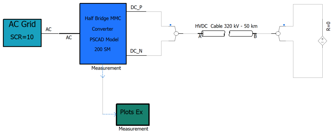
The system-level model used for the propagation study represents a single-end inverter-side MMC-HVDC converter station with a ±800 kV-class bipolar configuration. The MMC adopts the half-bridge submodule (SM) as its basic cell and arranges the SMs in a three-phase, six-arm topology, as shown in Figure 3. Each arm contains 200 series-connected SMs together with one arm reactor. The main electrical parameters are listed in Table 3.

3.2. Field Frequency-Response Measurement

The wideband models require terminal frequency-response data of the engineering-site primary equipment. The measurement practice follows the frequency-response analysis (FRA) principle standardized for power transformers [32]. The interpretation and application of FRA measurements are also consistent with the IEEE guide for frequency-response analysis [33]. The field sweep is a terminal frequency-response measurement performed on de-energized equipment. The measured responses are used as incremental terminal characteristics for the measured connection and equipment state. An HF-CBIS-V1 wideband impedance-spectroscopy analyzer records both magnitude and phase responses. The arm reactor is measured as a two-terminal device to obtain its port impedance over 1 kHz–30 MHz. For the single-phase converter transformer, the valve-side winding is measured (with the grid-side winding left open) using two port-impedance configurations, as illustrated in Figure 4. Here A and B denote the two terminals of the valve-side winding and the reference ground G is the transformer tank. The CM measurement short-circuits terminals A and B and measures the impedance from the short-circuited terminal to G, giving z 1 ( f ) . The DM measurement is performed directly between terminals A and B, giving z 2 ( f ) . The corresponding CM and DM impedances are then reconstructed using (6) and (8). The measured magnitude and phase responses provide the input data for the branch-parameter identification of the two wideband models.
Before the converter–transformer measurements, the HF-CBIS-V1 analyzer and the installed field leads were open- and short-circuit compensated at the lead ends close to the valve-side terminals. The compensation and zero check were repeated after changing between the CM and DM configurations. Shielded measurement leads were used, with their shields and guard reference connected to the transformer tank G. The lead and grounding geometry was kept fixed during each sweep. The grid-side bushings were disconnected from external busbars, cables, and test equipment and kept open, while the states of the other unused terminals remained unchanged. No additional signal-path connection to the tank was used during the z 2 measurement.

3.3. Model Verification

After the field frequency-response data are obtained, the identified wideband models are verified by comparing their calculated terminal responses with the measured responses in both magnitude and phase. For the arm reactor, the raw VF rational approximation and the synthesized PSCAD network are evaluated separately. The selected contains the ten retained parallel branches listed in Table 2. Its main inductive branch has L = 24.94 mH and R = 3.57 Ω . The accuracy of the raw rational approximation in the admittance domain is quantified by the mean relative magnitude error in dB,
ε ¯ Y = 20 log 10 1 M i = 1 M | Y fit ( f i ) Y meas ( f i ) | | Y meas ( f i ) | ,
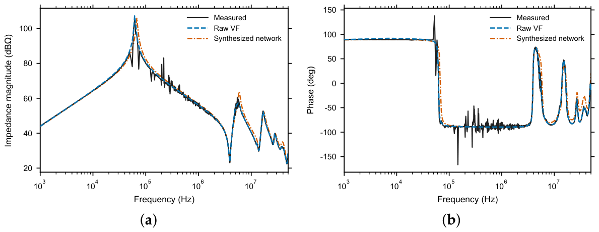
evaluated over the M frequency samples in the fitting band. Here, M is the dimensionless sample count, i is the sample index, f i is expressed in Hz , and Y fit and Y meas are expressed in S . Their relative difference and ε ¯ Y are dimensionless; the logarithmic error is reported in dB . The raw VF rational approximation gives ε ¯ Y 28.7 dB over 1 kHz–30 MHz. The synthesized PSCAD network is assessed separately in impedance magnitude and phase; its full-band mean relative magnitude error is 23.22%, and its phase mean absolute error is 12.70°. Over 1 kHz–2 MHz, which contains the main frequency range used in the station-level interpretation, the magnitude and phase errors are 7.13% and 2.87° for the raw VF model and 16.07% and 3.11° for the synthesized network. At 600.988 kHz, the corresponding errors are 1.77% and 1.43° for the raw VF model and 10.86% and 1.13° for the synthesized network. Larger pointwise magnitude residuals occur near narrow high-Q features, where a small frequency displacement produces a large relative error. All 20 fitted poles have negative real parts, and all retained circuit branches have positive physical parameters. Figure 5 distinguishes the measured response, rational order is N = 20 , and the synthesized equivalent network the raw rational approximation and the synthesized network. Together, the measured magnitude-and-phase agreement, stable poles, and positive physical branches provide direct equipment-level verification of the terminal model. The fitted poles collectively reconstruct the measured response, while physical interpretation is assigned to the retained passive branches.
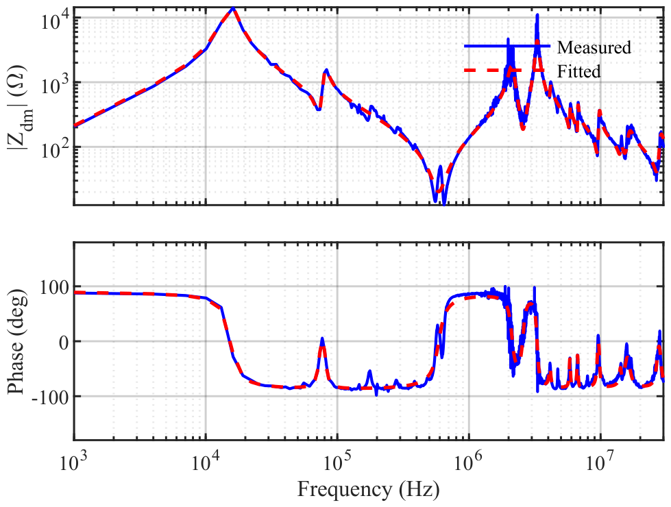
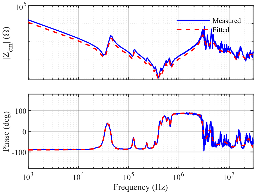
For the valve-side winding of the converter transformer, the DM response is reproduced with good agreement in the frequency range that is most relevant to the subsequent propagation study. The measured first main resonance is located at 16.15 kHz, while the fitted model gives 15.47 kHz, corresponding to a frequency deviation of about 4.2%. The fitted low-frequency leakage inductance is 33.77 mH, close to the value estimated from the measured low-frequency segment. The Foster I DM network preserves the dominant resonance and the phase transition around it (phase mean absolute error 5.5 ° ), as shown in Figure 6. Figure 7 shows that the Foster II CM network captures the main resonance-valley pattern and the overall phase variation of the measured CM impedance, which is sufficient for representing the CM path in the system-level HF propagation simulation.

3.4. PSCAD Implementation

The field-identified wideband models are integrated into the representative station-level PSCAD model described in Section 3.1. The synthesized arm-reactor network is connected in each bridge arm. The standard two-winding transformer retains the fundamental-frequency voltage transformation and magnetic coupling, while the identified differential-mode and common-mode networks are connected phase by phase at its valve-side terminals. These fixed-parameter R L C networks act as incremental terminal models for short-duration HF perturbations around the initialized station state. The submodule switching logic, capacitor-voltage states, circulating-current suppression, outer and inner control loops, DC cable, and AC-grid equivalent remain active in the station model. The simulation thus retains the switching and state evolution of the station while embedding linear wideband equipment subnetworks. The equipment terminal models are identified over 1 kHz–30 MHz, and the HF simulation uses a time step of 0.01 μ s.
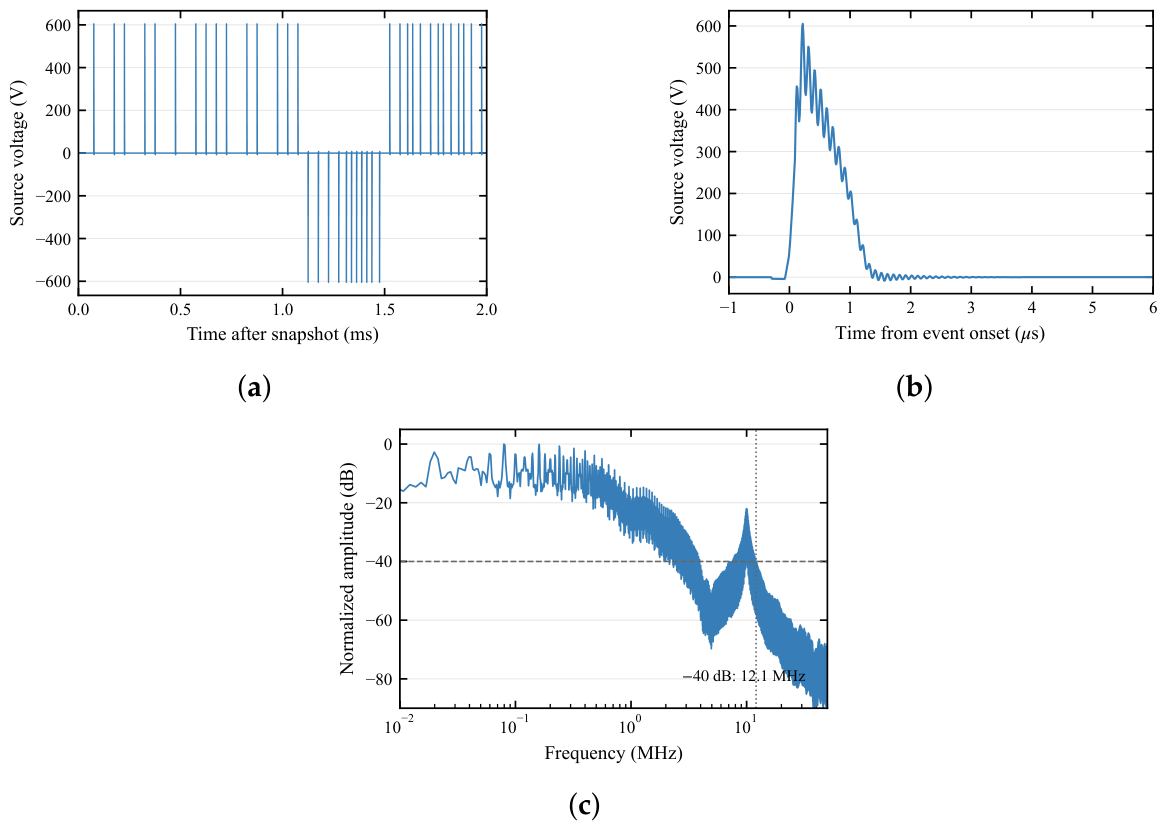
The valve-side excitation is constructed from the switching instants obtained from the nearest-level-control sequence. A parameterized single-event template contains a steep pulse front, a main pulse width of approximately 1.85 μ s, and a damped 10 MHz component. The same template is assigned the polarity of each switching event and scaled to a physical peak of 605.6 V. This construction provides the prescribed switching-transient boundary used in the station study, while the field frequency-response measurements supply the terminal impedances of the arm reactor and converter–transformer valve-side winding.
The source is implemented as a prescribed ideal-voltage boundary. The same terminal waveform is applied in the field-identified and conventional-equipment cases, so the paired simulations isolate the influence of the equipment terminal representation under an identical voltage excitation.
Figure 8 shows the resulting 2 ms source sequence. It contains 39 events, including 28 positive-polarity and 11 negative-polarity events, while the station switching and control dynamics remain active. A representative positive event with a rise time of approximately 0.225 μ s is selected for the detailed propagation plots so that adjacent events do not obscure the path response. The representative event has a normalized spectral magnitude of approximately 6.4 dB at 0.610 MHz, corresponding to about 48% of its maximum spectral amplitude. Its spectrum crosses the 40 dB level at approximately 12.1 MHz, so the source provides appreciable excitation across the frequency range used in the propagation analysis.
Two simulations start from the same 1.8-s snapshot and use identical equipment parameters, control states, and time steps. The source gain is set to 0.004 in the injection run and to zero in the baseline run. For any observed variable x ( t ) , the source-driven response is defined as
Δ x ( t ) = x inj ( t ) x 0 ( t ) ,
where t is expressed in seconds, and x inj , x 0 , and Δ x share the physical unit of the observed voltage or current. The subscripts denote the injection and zero-injection simulations, respectively. The six arm-level trajectories remain identical for 6.32 μ s after the first event, which covers the 0–4 μ s interval used for the time- and frequency-domain comparisons. The pre-event DC-side difference has an RMS value below 0.2 V.

4. Case Study: HF Signal Propagation

4.1. Simulation Configuration and Steady-State Operating Point

The representative source is connected between the lower terminal of the phase-A upper-arm reactor and the top terminal of the submodule string. From this port, one propagation path extends through the arm reactor toward the DC pole and cable, and a second path extends through the submodule string and the converter transformer toward the external AC network and the point of common coupling (PCC). The observation points at the arm-reactor terminal, DC-side node, transformer valve-side AC terminal, and PCC follow these two paths in physical order. This arrangement permits the source-front response, the local equipment-terminal response, and the propagation through the DC and AC networks to be examined within the same switching model.
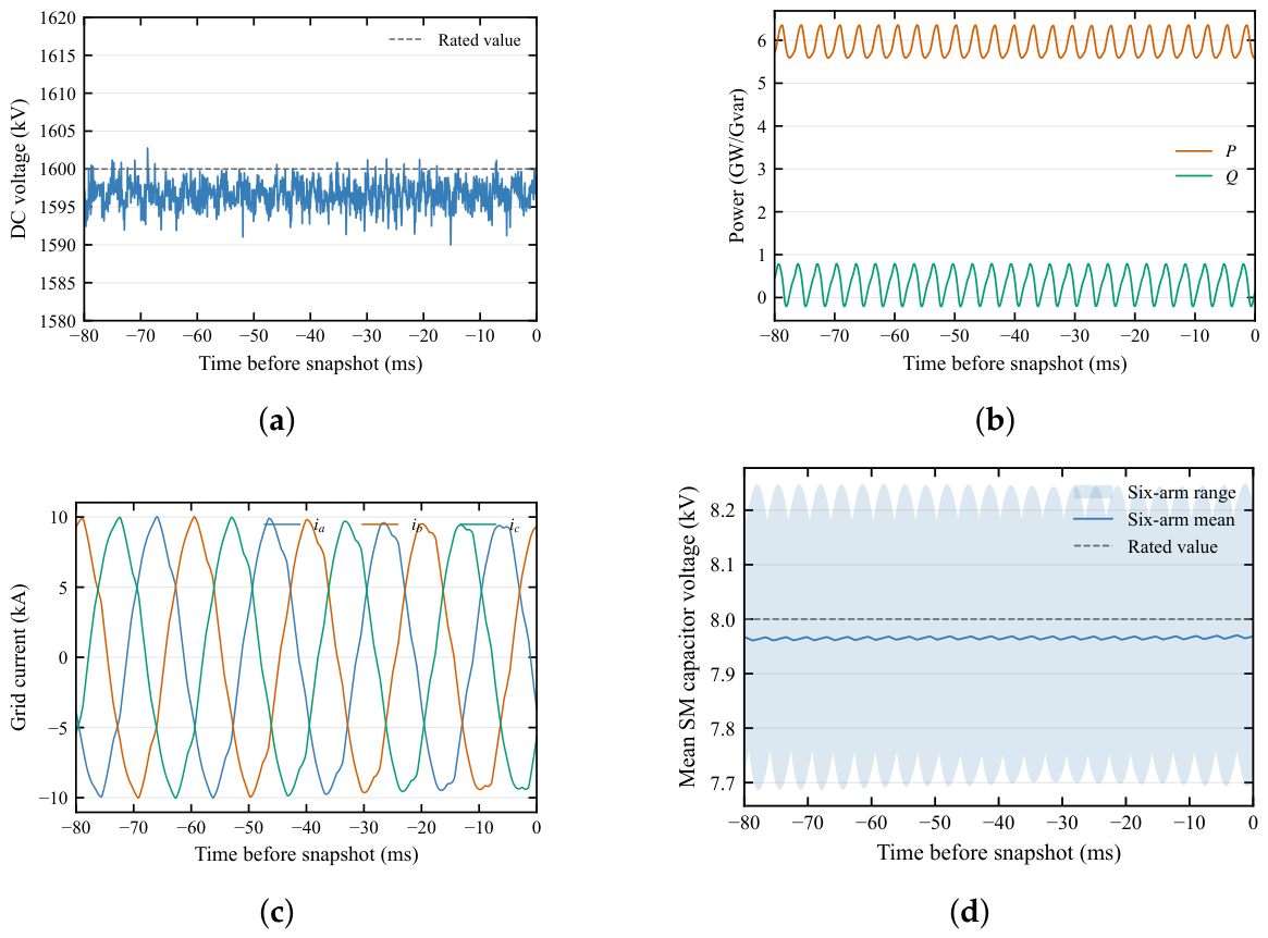
Before the HF source is enabled, the complete MMC-HVDC station is brought to the selected operating point. Figure 9 shows the final 80 ms before the snapshot. The pole-to-pole DC voltage remains close to 1600 kV, the transmitted active and reactive powers are stable, the grid-side three-phase currents are balanced, and the six arm-averaged submodule capacitor voltages remain centered near 8 kV. The snapshot retains the instantaneous submodule capacitor voltages, arm currents, controller states, and AC- and DC-network states. Both source-injection and zero-injection cases start from this common state, so the difference in Equation (13) isolates the response associated with the prescribed valve-side event during the common 0–4 μ s observation window.

4.2. Time-Domain Propagation of the Representative Event

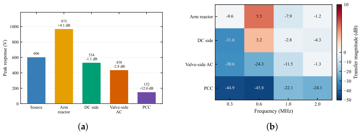
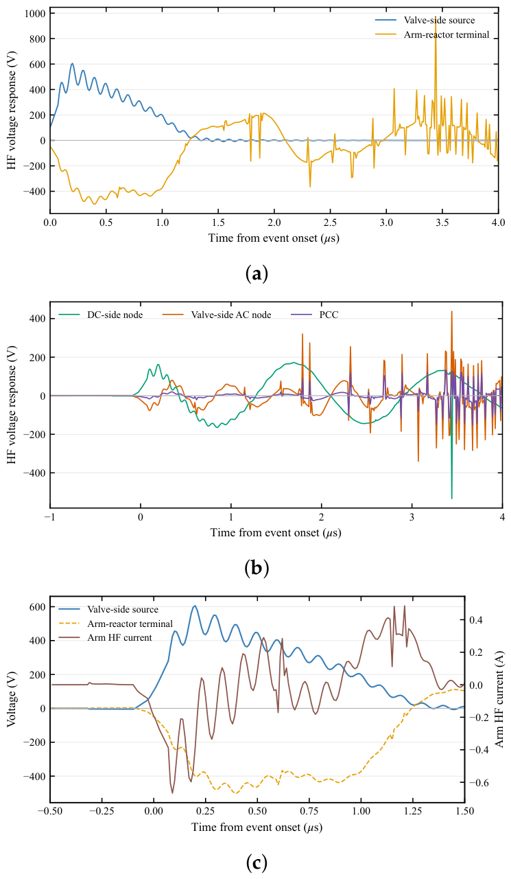
Figure 10a shows that propagation through the arm-reactor terminal is accompanied by pronounced waveform reshaping. The 605.6-V source produces an initial negative arm-reactor voltage followed by alternating extrema whose spacing is much shorter than the main source-pulse width. Over 0–4 μ s, the arm-reactor terminal reaches 972.6 V, corresponding to a 4.11 dB increase relative to the source peak. This peak occurs after the initial source front and identifies a local terminal-voltage response formed by the measured frequency-dependent reactor behavior together with the impedances connected on both sides of the observation port. The above-unity peak ratio reflects resonant voltage redistribution and passive energy exchange among the network storage elements.
The source-driven response reaches both sides of the converter. In Figure 10b, the DC-side, valve-side AC, and PCC peaks are 534.2, 438.4, and 151.9 V, respectively. These amplitudes are 88.2%, 72.4%, and 25.1% of the source peak and correspond to 1.09 , 2.81 , and 12.01 dB. The DC-side trace contains the strongest remote response and a sustained oscillatory tail. On the AC path, the valve-side terminal retains a distinct fast front, while the PCC peak is 34.7% of the valve-side AC peak. The associated 9.20 dB reduction is accumulated through the converter–transformer interface and the external AC-network equivalent. The aligned rapid changes in the valve-side AC and PCC traces confirm propagation across the transformer path, while their unequal amplitudes show that this path also reshapes the event.
Figure 10c resolves the first 1.5 μ s of the event. The arm-reactor voltage reverses polarity as the source rises, and the arm HF current reaches approximately 0.67 A during the initial front. The current excursion and the first reactor-voltage extremum occur within the source-front interval, after which both responses contain the faster oscillatory component. The sign of each plotted voltage follows its defined terminal reference, so the polarity reversal describes the voltage division across the source port and reactor terminal. The superimposed oscillations are consistent with the capacitive and resonant branches retained in the field-identified arm-reactor model [12]. Similar winding-capacitance effects are represented in wideband transformer models [9].

4.3. Frequency-Selective Propagation and DC-Side Oscillation

For a node k, the frequency-dependent transfer magnitude relative to the source is defined as
H k ( f ) = X k ( f ) X inj ( f ) ,
where k is the dimensionless node index, f is expressed in Hz , and X k ( f ) and X inj ( f ) are the voltage spectra of the node response and the source over the 0–4 μ s event interval. They use the same spectral normalization and physical unit, so H k is dimensionless. Figure 11 summarizes the time-domain peaks and the transfer magnitudes at 0.3, 0.6, 1.0, and 2.0 MHz.
The numerical values in Table 4 demonstrate that the relative ordering of the observation points changes with frequency. At 0.3 MHz, the arm-reactor terminal remains close to the source level, while the three remote nodes are reduced by more than 30 dB. At 0.6 MHz, the arm-reactor and DC-side responses rise to + 5.52 and + 3.15 dB, while the valve-side AC and PCC responses remain at 24.28 and 45.80 dB. At 1.0 MHz, the DC-side response is only 2.84 dB below the source, whereas the PCC response is 22.07 dB below it. At 2.0 MHz, the arm-reactor, DC-side, and valve-side AC responses are 1.25 , 4.28 , and 1.34 dB, but the PCC response remains at 24.13 dB. The station response is thus frequency selective at each observation point and cannot be represented by one propagation coefficient over the analyzed band.
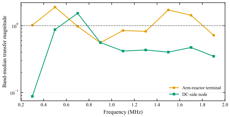
Figure 12 resolves the DC propagation path in 200 kHz bands. The arm-reactor terminal has local maxima in the 0.4–0.6 and 1.4–1.8 MHz regions. The DC-side node is most strongly coupled in the 0.6–0.8 MHz band, where its band-median transfer magnitude is 1.53. Outside this band, its transfer magnitude decreases to 0.35–0.87 over 0.4–2.0 MHz and to 0.087 in the 0.2–0.4 MHz band. The unequal reactor-terminal and DC-node curves show that the arm-reactor response alone does not determine the remote DC voltage; the connected DC network selects and redistributes the frequency components that cross the reactor terminal.
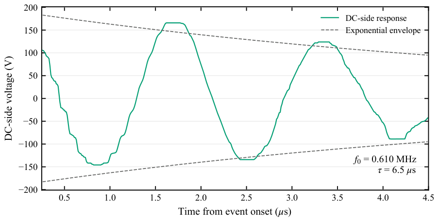
The DC-side response contains a dominant damped oscillation after the pulse front. The adjacent extrema in Figure 13 give an oscillation frequency of approximately 0.610 MHz and a decay time constant of approximately 6.5 μ s. The representative event retains approximately 48% of its maximum spectral amplitude at 0.610 MHz, and the DC-side spectral enhancement is centered in the 0.6–0.8 MHz band. The appreciable source component, the adjacent-extrema estimate, and the transfer enhancement consistently identify the same frequency range.
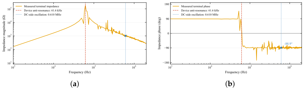
Figure 14 distinguishes an isolated-equipment feature from the complete-system response. The principal arm-reactor anti-resonance occurs at 61.6 kHz, almost one decade below the 0.610 MHz DC oscillation. At 0.610 MHz, the measured arm-reactor terminal impedance is approximately 1.01 k Ω and its phase is 88.9 ° , so the terminal behavior is predominantly capacitive. The oscillation is thus not the isolated reactor anti-resonance; its frequency is set by the combined frequency-dependent impedances of the converter arm and connected DC network. System-impedance studies and field-informed MMC-HVDC models likewise show that high-frequency resonance frequencies depend on the interaction between equipment parasitic characteristics and the connected network [8,13,26]. The agreement between the time-domain oscillation, the source spectrum, and the frequency-domain transfer supports this equipment–network interpretation.
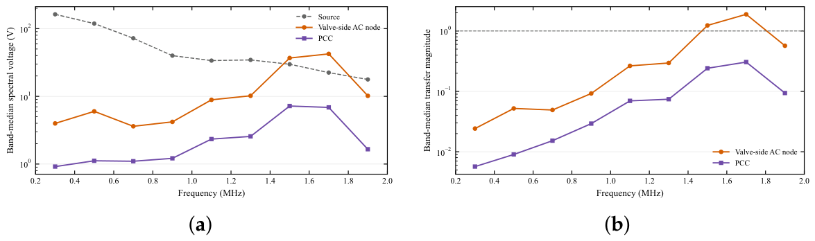
The AC-side frequency bands are examined separately in Figure 15. Over 0.3–0.9 MHz, the valve-side AC transfer magnitude ranges from 0.024 to 0.092, and the PCC transfer ranges from 0.0057 to 0.029. Over 1.1–1.9 MHz, the valve-side AC transfer rises to 0.265–1.888, with local enhancement in the 1.5 and 1.7 MHz bands; the PCC transfer remains between 0.070 and 0.306. The two curves retain the same broad increase toward 1.5–1.7 MHz, which indicates that these components cross the transformer interface and remain identifiable at the PCC. Their magnitudes are not preserved: the PCC-to-valve-side ratio is approximately 0.20 in the 1.5 MHz band and 0.16 in the 1.7 MHz band. The transformer and external AC network substantially reduce the 0.3–0.9 MHz components and impose additional attenuation on the higher-frequency content that reaches the PCC.

4.4. Controlled Comparison with Conventional Lumped Equipment Models

A controlled model comparison quantifies the contribution of the field-identified terminal networks. The wideband case uses the synthesized arm-reactor and converter–transformer terminal models described in Section 2.1 and Section 2.2. The conventional case uses the corresponding fundamental-frequency lumped representations. The converter topology, control system, DC cable, AC-grid equivalent, operating-point snapshot, 0.01 μ s time step, and valve-side source waveform are unchanged. Thus, the equipment representation is the only prescribed difference between the two station models.
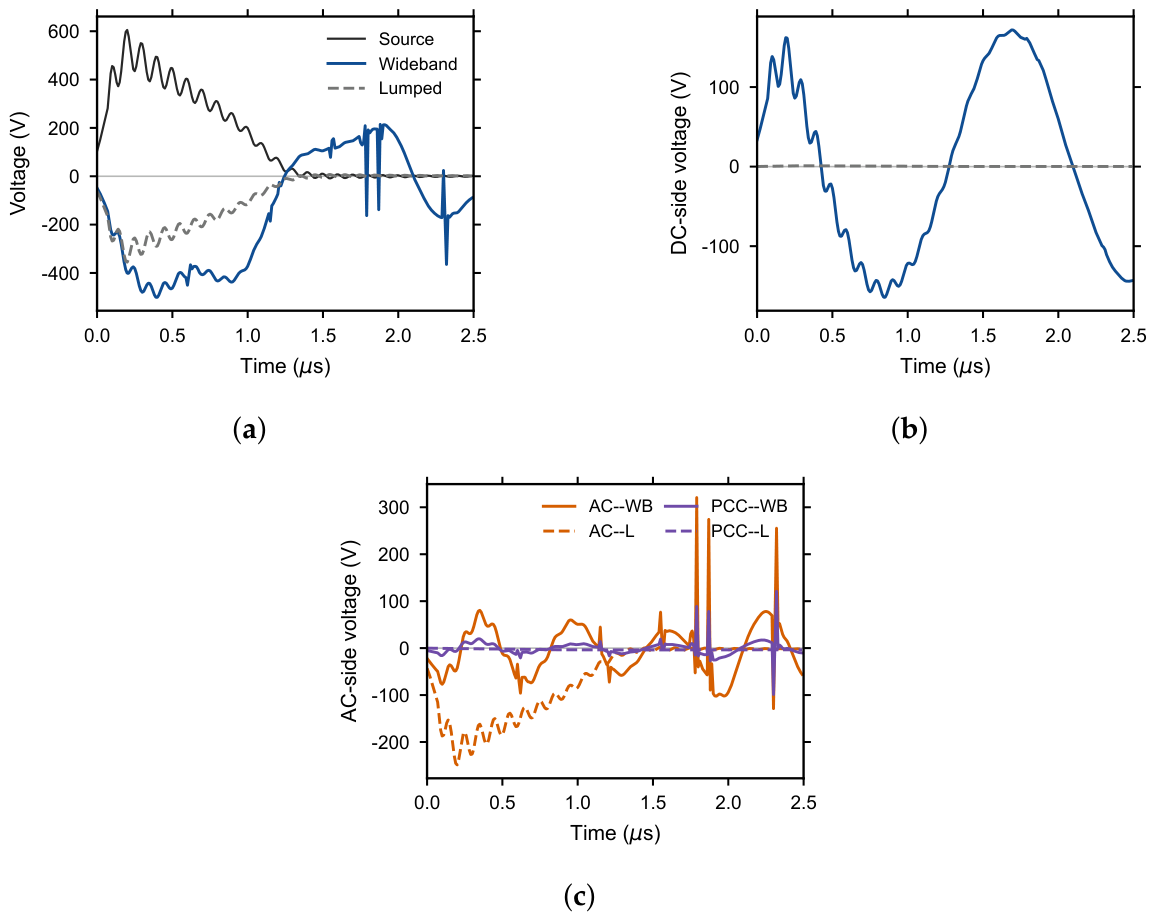
Each equipment case is evaluated through its own source-injection and zero-injection pair. The comparison signals are Δ x WB = x WB , inj x WB , 0 and Δ x L = x L , inj x L , 0 , where WB and L denote the field-identified wideband and conventional lumped models. The two paired source waveforms have the same 605.6-V peak, and their maximum pointwise difference is below 2.1 × 10 8 V. The first change in submodule insertion states between the injection and zero-injection runs occurs at 6.30 μ s for the wideband model and 2.83 μ s for the lumped model. The controlled comparison is consequently restricted to 0–2.5 μ s after the event onset, which lies within the control-identical interval of both pairs. The 0–4 μ s window used for the wideband propagation analysis in Section 4.2 and Section 4.3 is retained for those results.
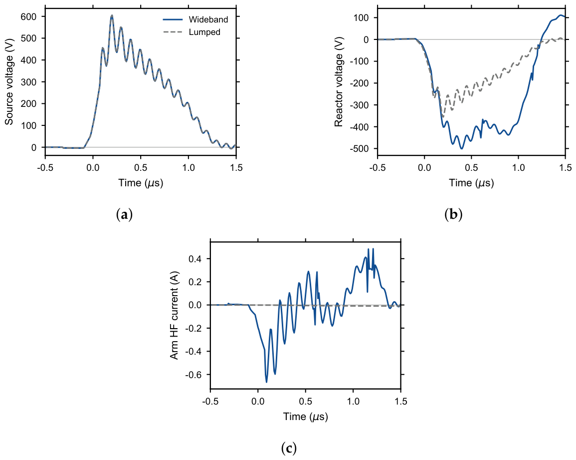
Figure 16 shows that the same source waveform produces different responses once it enters the station network. The arm-reactor-terminal peak is 500.9 V with the field-identified model and 355.6 V with the lumped model, a difference of 2.98 dB. The corresponding DC-side peaks are 171.9 and 1.23 V, giving a 42.88 dB difference. On the AC path, the valve-side peaks are 320.9 and 248.8 V, while the PCC peaks are 121.4 and 3.93 V. The wideband-to-lumped peak changes are 2.21 dB at the valve-side AC node and 29.79 dB at the PCC. The model effect is thus path-dependent: the two valve-side AC peaks remain of the same order, whereas the remote DC and PCC responses change by more than one order of magnitude.
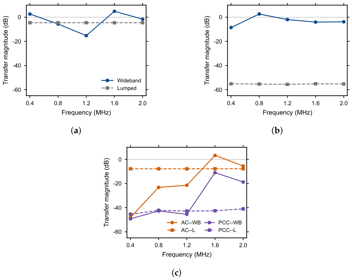
The spectral ratios in Figure 17 show that the equipment representation changes both the magnitude and the frequency dependence of the propagation paths. At 0.8 MHz, the reactor-terminal transfers are 5.65 and 4.56 dB for the wideband and lumped models, respectively, but the DC-side transfers are + 2.66 and 55.39 dB. At 1.6 MHz, the wideband reactor, valve-side AC, and PCC transfers are + 4.94 , + 3.33 , and 11.00 dB, compared with 4.57 , 7.80 , and 42.57 dB for the lumped model. The wideband model does not give a uniformly larger response. For example, its valve-side AC transfer at 0.8 MHz is 23.17 dB, below the 7.81 dB obtained with the lumped representation. The measured terminal networks alter the frequency-dependent voltage division and can change the relative importance of the DC, valve-side AC, and PCC observation points.
The source overlap in Figure 18a verifies that the differences in Figure 16 and Figure 17 do not originate from unequal excitations. The two reactor responses initially follow the same negative front and then separate as the field-identified resonant and capacitive paths become active. Over 0–2.5 μ s, the arm HF-current peaks are 1.875 A with the wideband model and 0.0091 A with the lumped model. This difference accompanies the stronger voltage redistribution toward the DC-side and PCC nodes in the field-identified case.
Table 5 summarizes the controlled comparison. The close reactor and valve-side AC peak levels at some points coexist with much larger differences at the DC side and PCC. The discrete transfer values also show that the effect changes with frequency. A conventional lumped representation can consequently preserve the imposed source waveform while changing the predicted path ranking and suppressing station-level components produced by the measured terminal networks.

4.5. Discussion

The results distinguish the roles of the main elements along the propagation path. The arm-reactor terminal exhibits the largest time-domain peak, but the remote DC-side response is governed by the interaction of that terminal behavior with the connected DC network. On the AC path, the converter–transformer valve-side model and the external AC network determine how much of each frequency band reaches the PCC. The 0.3–0.9 MHz components are strongly reduced, while a larger fraction of the 1.5–1.7 MHz content remains identifiable at the valve-side AC terminal and PCC. The observed waveform at any one point is consequently a path-dependent result, not a scaled copy of the valve-side source.
This distinction has practical implications for station-level HF assessment. A measurement point selected only from physical distance may miss the node at which a particular frequency band is enhanced. The arm-reactor terminal is important for local voltage stress, the DC-side node captures the dominant 0.610 MHz oscillation, and the valve-side AC and PCC nodes describe the components that cross the transformer path. These locations support different insulation-coordination, electromagnetic-compatibility, and monitoring questions. IGBT switching-transient models provide the device-level source context [3], and MMC electromagnetic-interference models show that submodule switching states generate conducted-HF components [4]. Converter–transformer stray capacitances can also affect grid-side HF propagation paths [7].
Low-frequency lumped or averaged MMC-HVDC models reproduce fundamental-frequency operation and slow transients [34]. Their equipment representations do not contain the measured capacitive and resonant branches that shape terminal behavior over the kHz-to-MHz range. The controlled comparison in Section 4.4 holds the operating state, source waveform, switching states, and external network constant over the analyzed interval. The conventional model gives reactor and valve-side AC peaks of the same order as the field-identified model, but its DC-side and PCC peaks are lower by 42.88 and 29.79 dB. The frequency-domain differences also change sign across the evaluated points. These results indicate that the terminal representation changes the predicted path ranking and frequency-dependent voltage division, not simply the overall response scale.
Published implementations show that the measurement-to-network workflow applies across different equipment ratings and terminal formulations. Holdyk et al. combined measured transformer terminal admittance, vector fitting, passivity enforcement, and time-domain validation [23]. Gustavsen and Tandstad integrated a measured passive six-terminal transformer model into PSCAD, EMTP-RV, and ATP for voltage-transfer and network-interaction studies [24], while Ren et al. synthesized physical ladder networks from measured transformer-winding admittance [25]. These implementations share the same sequence used here: terminal-response measurement, stable network synthesis, and integration into the surrounding EMT system. The measured ports, retained branch count, and simulation bandwidth are selected for each target installation.

5. Conclusions

A field-measurement-based wideband modeling workflow has been established for the arm reactor and the converter–transformer valve-side winding of an MMC-HVDC station. The admittance-domain arm-reactor fit and passive parallel synthesis reproduce the measured terminal response over 1 kHz–30 MHz. The transformer differential-mode and common-mode responses are reconstructed from two field measurements and synthesized as a Foster I/II hybrid π network. Both equipment models are integrated into a station-level PSCAD platform with the converter switching and controls retained.
Paired injection and zero-injection simulations isolate the response of a representative 605.6-V valve-side event. Over 0–4 μ s, the arm-reactor terminal reaches 972.6 V, while the DC-side, valve-side AC, and PCC peaks are 534.2, 438.4, and 151.9 V. The corresponding changes relative to the source are + 4.11 , 1.09 , 2.81 , and 12.01 dB. The DC-side response contains a dominant oscillation near 0.61 MHz, and the AC/PCC transfer changes markedly over 0.2–2.0 MHz. In the separate 0–2.5 μ s control-identical comparison, the field-identified model gives DC-side and PCC peaks 42.88 and 29.79 dB above those obtained with conventional lumped equipment. The comparison also contains frequency points at which the lumped response is larger, confirming that the terminal representation changes frequency-dependent voltage division and path ranking.

Author Contributions

Conceptualization, B.Y. and H.M.; methodology, T.B.; software, T.B. and Z.L.; validation, B.Y., Y.J., L.L. and G.C.; formal analysis, T.B. and M.S.; investigation, M.S.; resources, J.S. and H.M.; data curation, T.B. and M.S.; writing—original draft preparation, T.B.; writing—review and editing, H.M. and B.Y.; visualization, T.B. and Z.L.; supervision, H.M.; project administration, B.Y. and H.M.; funding acquisition, B.Y. and H.M. All authors have read and agreed to the published version of the manuscript.

Funding

This research was funded by the Science and Technology Project of State Grid Zhejiang Electric Power Co., Ltd., grant number 5211DS250009 (Project Name: Research on Anti-interference Partial Discharge Detection Technology and Device Development for Flexible DC Harmonics of UHV Large Capacity Converter Transformers under Step-by-Step Commissioning Mode). The APC was funded by the Science and Technology Project of State Grid Zhejiang Electric Power Co., Ltd.

Data Availability Statement

The field-measured frequency-response dataset and the MATLAB parameter-identification scripts used in this study are openly available on GitHub at https://github.com/wxt18757928900-lgtm/MMC-HVDC-data (accessed on 24 August 2026). The PSCAD case data and the plotting scripts used for the station-level propagation figures are available from the corresponding author upon reasonable request.

Conflicts of Interest

Authors B.Y., Y.J., and L.L. ware employed by the Research Institute of Electric Power Science, State Grid Zhejiang Electric Power Co., Ltd. Author J.S. was employed by Construction Branch, State Grid Zhejiang Electric Power Co., Ltd. Author G.C. was employed by State Grid Zhejiang Electric Power Co., Ltd. The authors declare that this study received funding from Science and Technology Project of State Grid Zhejiang Electric Power Co., Ltd. The funder was not involved in the study design, collection, analysis, interpretation of data, the writing of this article or the decision to submit it for publication.

Abbreviations

The following abbreviations are used in this manuscript:
ACAlternating current
CMCommon mode
DCDirect current
DFTDiscrete Fourier transform
DMDifferential mode
EMIElectromagnetic interference
EMTElectromagnetic transient
FRAFrequency-response analysis
HFHigh frequency
HVDCHigh-voltage direct current
IGBTInsulated-gate bipolar transistor
MMCModular multilevel converter
MMC-HVDCModular multilevel converter-based high-voltage direct current
PCCPoint of common coupling
PSCADPower systems computer-aided design
RLCResistor–inductor–capacitor
sFRASweep frequency-response analysis
SMSubmodule
VFVector fitting

References

  1. Lesnicar, A.; Marquardt, R. An Innovative Modular Multilevel Converter Topology Suitable for a Wide Power Range. In Proceedings of the IEEE Bologna Power Tech Conference Proceedings, Bologna, Italy, 23–26 June 2003; Volume 3, pp. 272–277. [Google Scholar] [CrossRef] [Scilit]
  2. Pan, E.; Yue, B.; Li, X.; Zhao, Z.; Zhu, Q. Integration technology and practice for long-distance offshore wind power in China. Energy Convers. Econ. 2020, 1, 4–19. [Google Scholar] [CrossRef] [Scilit]
  3. Xu, Y.; Ho, C.N.M.; Ghosh, A.; Muthumuni, D. An Electrical Transient Model of IGBT-Diode Switching Cell for Power Semiconductor Loss Estimation in Electromagnetic Transient Simulation. IEEE Trans. Power Electron. 2020, 35, 2979–2989. [Google Scholar] [CrossRef] [Scilit]
  4. Sun, T.; Pei, X.; Shan, Y.; Pei, J.; Jiang, D. Submodule Switching-State Based EMI Modeling and Mixed-Mode EMI Phenomenon in MMC. IEEE Trans. Power Electron. 2023, 38, 1831–1843. [Google Scholar] [CrossRef] [Scilit]
  5. Wang, Z.; Li, H.; Chu, Z.; Zhang, C.; Yang, Z.; Shao, T.; Hu, Y. A Review of EMI Research in Modular Multilevel Converter for HVDC Applications. IEEE Trans. Power Electron. 2022, 37, 14482–14498. [Google Scholar] [CrossRef] [Scilit]
  6. Zhu, R.; Lin, N.; Dinavahi, V.; Liang, G. An Accurate and Fast Method for Conducted EMI Modeling and Simulation of MMC-Based HVdc Converter Station. IEEE Trans. Power Electron. 2020, 35, 4689–4702. [Google Scholar] [CrossRef] [Scilit]
  7. Li, G.; Ye, H.; Bin, Z. High-frequency oscillation mechanism analysis of wind farm-side MMC station considering converter transformer stray capacitance. Int. J. Electr. Power Energy Syst. 2023, 153, 109179. [Google Scholar] [CrossRef] [Scilit]
  8. Hu, Y.; Li, Y.; Li, Y.; Chen, J.; Zhang, Y. Modeling and Parameter Identification of Converter Transformer for High-Frequency Resonance Problem of Flexible DC Converter Station. Trans. China Electrotech. Soc. 2024, 39, 7154–7166. (In Chinese) [Google Scholar] [CrossRef]
  9. Nasirpour, F.; Heidary, A.; Niasar, M.G.; Lekić, A.; Popov, M. High-frequency transformer winding model with adequate protection. Electr. Power Syst. Res. 2023, 223, 109637. [Google Scholar] [CrossRef] [Scilit]
  10. Das, A.K.; Fernandes, B.G. Estimation of the Resonance Frequencies Using an Electrostatic Energy Based Capacitance Model of a Two-Winding Medium/High-Frequency Transformer. IEEE Trans. Ind. Appl. 2022, 58, 5301–5316. [Google Scholar] [CrossRef] [Scilit]
  11. Zhao, H.; Luan, S.; Shen, Z.; Hanson, A.J.; Gao, Y.; Dalal, D.N.; Wang, R.; Zhou, S.; Munk-Nielsen, S. Rethinking Basic Assumptions for Modeling Parasitic Capacitance in Inductors. IEEE Trans. Power Electron. 2022, 37, 8281–8289. [Google Scholar] [CrossRef] [Scilit]
  12. Lan, Y.; Yang, L.; Zhang, X.; Chen, Q.; Zheng, Z. Calculation Model of Parasitic Capacitance for High-Frequency Inductors and Transformers. IEEE Access 2023, 11, 143182–143189. [Google Scholar] [CrossRef] [Scilit]
  13. Dai, F.; Zeng, D.; Liu, S.; Wang, G. A practical impedance modeling method of MMC-HVDC transmission system for medium- and high-frequency resonance analysis. Electr. Power Syst. Res. 2022, 212, 108636. [Google Scholar] [CrossRef] [Scilit]
  14. Guo, H. Impedance and Stability Analysis of Voltage-Source Converter Interconnection Based on a Universal Admittance Model. IEEE Trans. Power Electron. 2020, 35, 10064–10077. [Google Scholar] [CrossRef]
  15. Wang, J.; Chen, W.; Liu, Y.; Fu, C.; Ye, Y.; Feng, J. High-frequency Resonance Analysis and Impedance Reshaping Control of MMC-HVDC System Based on Frequency Coupling Impedance Model. J. Mod. Power Syst. Clean Energy 2024, 12, 646–657. [Google Scholar] [CrossRef] [Scilit]
  16. Guo, C.; Du, D.; Cheng, H.; Gan, F. A Frequency Estimation-Based Adaptive Mitigation Approach for High-Frequency Oscillation in MMC-HVDC System. IEEE Trans. Power Syst. 2024, 39, 5509–5521. [Google Scholar] [CrossRef] [Scilit]
  17. Morched, A.; Marti, L.; Ottevangers, J. A high frequency transformer model for the EMTP. IEEE Trans. Power Deliv. 1993, 8, 1615–1626. [Google Scholar] [CrossRef] [Scilit]
  18. Gustavsen, B. Wide Band Modeling of Power Transformers. IEEE Trans. Power Deliv. 2004, 19, 414–422. [Google Scholar] [CrossRef]
  19. Zheng, Y.M.; Wang, Z.J. Determining the Broadband Loss Characteristics of Power Transformer Based on Measured Transformer Network Functions and Vector Fitting Method. IEEE Trans. Power Deliv. 2013, 28, 2456–2464. [Google Scholar] [CrossRef] [Scilit]
  20. Gustavsen, B.; Semlyen, A. Rational Approximation of Frequency Domain Responses by Vector Fitting. IEEE Trans. Power Deliv. 1999, 14, 1052–1061. [Google Scholar] [CrossRef] [Scilit]
  21. Gustavsen, B. Improving the Pole Relocating Properties of Vector Fitting. IEEE Trans. Power Deliv. 2006, 21, 1587–1592. [Google Scholar] [CrossRef] [Scilit]
  22. Gustavsen, B.; Semlyen, A. Enforcing passivity for admittance matrices approximated by rational functions. IEEE Trans. Power Syst. 2001, 16, 97–104. [Google Scholar] [CrossRef]
  23. Holdyk, A.; Gustavsen, B.; Arana, I.; Holboell, J. Wideband Modeling of Power Transformers Using Commercial sFRA Equipment. IEEE Trans. Power Deliv. 2014, 29, 1446–1453. [Google Scholar] [CrossRef] [Scilit]
  24. Gustavsen, B.; Tandstad, B. Wideband Modeling of a 45-MVA Generator Step-Up Transformer for Network Interaction Studies. Electr. Power Syst. Res. 2017, 142, 47–57. [Google Scholar] [CrossRef] [Scilit]
  25. Ren, F.; Zhang, H.; Liu, Y.; Ji, S.; Li, Q. Ladder Network Synthesis in Wide Frequency Range for Transformer Winding From Its Driving-Point Admittance Data. IEEE Trans. Power Deliv. 2022, 37, 1370–1379. [Google Scholar] [CrossRef] [Scilit]
  26. Shen, H.; Dongye, Z.; Qi, L.; Wang, M.; Zhang, X.; Qiu, P.; Wei, X. Modeling of High-frequency Electromagnetic Oscillation for DC Fault in MMC-HVDC Systems. CSEE J. Power Energy Syst. 2023, 9, 1151–1160. [Google Scholar] [CrossRef] [Scilit]
  27. Lin, L.; Zeng, Q.; Zhu, J.; Shi, X.; Hu, J. High-Frequency Oscillation Mechanism Analysis and Suppression Strategy of Grid-Forming Control MMC-HVDC. IEEE Trans. Power Del. 2023, 38, 1588–1600. [Google Scholar] [CrossRef] [Scilit]
  28. Xu, J.; Zhu, Y.; Liu, Y.; Tian, Z.; Zhao, C.; Li, G. Electromagnetic Transient Modeling and Simulation Method for Internal Faults in Permanent Magnet Synchronous Generators. J. Mod. Power Syst. Clean Energy 2026, 14, 907–919. [Google Scholar] [CrossRef] [Scilit]
  29. Zhao, H.; Lan, J.; Chen, W.; Wang, Y.; Chen, Y.; Yuan, Y. A New High-Ratio-Transformer Based Soft Open Point with Mixed-Frequency Modulation Method. IEEE Trans. Power Electron. 2026, 41, 17402–17417. [Google Scholar] [CrossRef] [Scilit]
  30. Sanathanan, C.K.; Koerner, J. Transfer function synthesis as a ratio of two complex polynomials. IEEE Trans. Autom. Control 1963, 8, 56–58. [Google Scholar] [CrossRef] [Scilit]
  31. Gustavsen, B. Wideband Transformer Modeling Including Core Nonlinear Effects. IEEE Trans. Power Deliv. 2016, 31, 219–227. [Google Scholar] [CrossRef] [Scilit]
  32. IEC 60076-18:2012; Power Transformers–Part 18: Measurement of Frequency Response. International Electrotechnical Commission: Geneva, Switzerland, 2012.
  33. IEEE Std C57.149-2024; IEEE Guide for the Application and Interpretation of Frequency Response Analysis for Oil-Immersed Transformers. IEEE: New York, NY, USA, 2024.
  34. Saad, H.; Peralta, J.; Dennetière, S.; Mahseredjian, J.; Jatskevich, J.; Martinez, J.A.; Davoudi, A.; Saeedifard, M.; Sood, V.; Wang, X.; et al. Dynamic Averaged and Simplified Models for MMC-Based HVDC Transmission Systems. IEEE Trans. Power Deliv. 2013, 28, 1723–1730. [Google Scholar] [CrossRef] [Scilit]
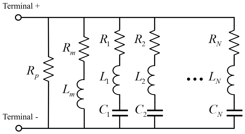
Figure 1. Simplified topology of the implemented wideband arm-reactor equivalent circuit, consisting of a shunt resistance, a main inductive branch and multiple fitted series R L C branches connected in parallel.
Electronics 15 03860 g001
Figure 2. Wideband terminal model of the converter–transformer valve-side winding: (a) DM/CM decomposition, (b) Foster I synthesis of the differential-mode impedance Z dm , and (c) Foster II synthesis of the common-mode impedance Z cm .
Electronics 15 03860 g002
Figure 3. Single-line topology of the representative ±800 kV-class MMC-HVDC converter-station model used in the PSCAD propagation study.
Electronics 15 03860 g003
Figure 4. Field measurement configurations for the valve-side winding port impedances (grid-side winding open): (a) CM measurement for z 1 and (b) DM measurement for z 2 .
Electronics 15 03860 g004
Figure 5. Arm-reactor terminal-response verification over 1 kHz–30 MHz: (a) impedance magnitude and (b) phase. The field-measured response is compared with the raw VF rational approximation and the synthesized passive network implemented in PSCAD.
Electronics 15 03860 g005
Figure 6. Measured and fitted DM impedance responses of the converter–transformer valve-side winding.
Electronics 15 03860 g006
Figure 7. Measured and fitted CM impedance responses of the converter–transformer valve-side winding.
Electronics 15 03860 g007
Figure 8. Valve-side HF excitation used in the station simulation: (a) The complete 2 ms event sequence; (b) the representative positive-polarity event; and (c) the normalized amplitude spectrum.
Electronics 15 03860 g008
Figure 9. Steady-state operating point before the HF propagation case: (a) DC voltage; (b) transmitted active and reactive powers; (c) grid-side three-phase currents; and (d) the six-arm range and mean of the arm-averaged submodule capacitor voltages.
Electronics 15 03860 g009
Figure 10. Time-domain response of the representative event: (a) valve-side source and arm-reactor terminal voltages over 0–4 μ s; (b) DC-side, valve-side AC, and PCC node voltages from 1 to 4 μ s; and (c) source voltage, arm-reactor terminal voltage, and arm HF current during the initial front.
Electronics 15 03860 g010
Figure 11. Propagation summary for the representative event: (a) Peak responses over 0–4 μ s and their changes relative to the source; and (b) voltage-transfer magnitudes at four representative frequencies.
Electronics 15 03860 g011
Figure 12. Band-median voltage-transfer magnitudes at the arm-reactor terminal and DC-side node over 0.2–2.0 MHz. The dashed line denotes unity transfer.
Electronics 15 03860 g012
Figure 13. Dominant damped oscillation in the DC-side response. The fitted oscillation frequency is approximately 0.610 MHz and the decay time constant is approximately 6.5 μ s.
Electronics 15 03860 g013
Figure 14. Relation between the measured arm-reactor terminal response and the station-level DC oscillation: (a) Impedance magnitude and (b) impedance phase. The isolated-device anti-resonance and the station oscillation are marked separately.
Electronics 15 03860 g014
Figure 15. AC-side frequency-band response over 0.2–2.0 MHz: (a) Source, valve-side AC, and PCC spectral-voltage amplitudes; (b) valve-side AC and PCC transfer magnitudes relative to the source. Values are summarized in 200 kHz bands.
Electronics 15 03860 g015
Figure 16. Controlled time-domain comparison over the common 0–2.5 μ s interval: (a) Valve-side source and arm-reactor-terminal responses, (b) DC-side response, and (c) valve-side AC and PCC responses. Solid curves denote the field-identified wideband model; dashed curves denote the conventional lumped model.
Electronics 15 03860 g016
Figure 17. Discrete voltage-transfer magnitudes obtained from the common 0–2.5 μ s interval: (a) Arm-reactor terminal, (b) DC-side node, and (c) valve-side AC and PCC nodes. The 2.5 μ s record gives a 0.4 MHz discrete Fourier transform (DFT) spacing. Circles denote the field-identified wideband model, and squares denote the conventional lumped model.
Electronics 15 03860 g017
Figure 18. Initial-front comparison from 0.5 to 1.5 μ s: (a) Overlapping source voltages, (b) arm-reactor-terminal voltages, and (c) arm HF currents. The maximum difference between the two source traces is below 2.1 × 10 8 V.
Electronics 15 03860 g018
Table 1. Comparison of the present method with representative and reviewer-recommended studies.
StudySystem or ObjectModel BasisMain FocusEvidence or Scale
Lin et al. [27]Grid forming MMC-HVDC networkDynamic phasor small-signal modelHFO related to control1.38/1.56 kHz; RT-LAB
Shen et al. [26]MMC-HVDC DC fault clearingParasitic circuit and staged equationsOscillation during fault stages200 kV short circuit test
Measured transformer models [8,23,24,25]Transformer terminal networksMeasured response and passive synthesisEquipment and network response45 MVA example; 5 Hz–10 MHz; EMT
Xu et al. [28]PMSG internal faultsBackward Euler nodal EMTFault and system integration2 MW unit/200 MW farm; MATLAB benchmark
Zhao et al. [29]High-ratio transformer soft open pointTopology and mixed frequency modulationPower flow and voltage balancing190 V/3.7 kW experiment
Present workArm reactor, converter transformer, and stationField response, passive synthesis, and PSCADPropagation paths of switching disturbances±800 kV station field data; 1 kHz–30 MHz sweep
Table 2. Synthesized wideband branches of the arm-reactor equivalent network.
#TypeR ( Ω )L (H)C (F) f 0 (MHz)
1 R L C 26.8 4.00 × 10 7 2.38 × 10 11 51.6
2 R L C 19.0 8.93 × 10 7 1.23 × 10 11 48.0
3 R L C 65.0 1.42 × 10 6 1.41 × 10 11 35.6
4 R L C 69.7 4.52 × 10 6 8.07 × 10 12 26.4
5 R L C 39.4 5.12 × 10 6 2.51 × 10 11 14.0
6 R L C 283 1.30 × 10 5 1.27 × 10 11 12.4
7 R L C 1.48 × 10 3 2.00 × 10 4 5.01 × 10 12 5.03
8 R L C 15.2 1.38 × 10 5 1.20 × 10 10 3.91
9Main RL 3.57 2.49 × 10 2
10Damping R 2.00 × 10 5
Branches 1–8 are series- R L C resonant branches; branch 9 is the main RL branch and branch 10 the global damping resistance. All branches are connected in parallel.
Table 3. Main electrical parameters of the representative MMC-HVDC system-level model.
ItemValue
ConfigurationSingle-end inverter, ±800 kV-class bipolar
Rated power S N 8 GW
Pole-to-pole DC voltage1600 kV
AC-side line voltage515 kV
Rated DC current≈5000 A
Submodule typeHalf-bridge
Submodules per arm N SM = 200
Rated SM capacitor voltage V C = 8 kV
Table 4. Time-domain peak responses and frequency-dependent transfer magnitudes for the representative event. The peaks and spectra use the common 0–4 μ s event interval.
Observation PointPeak (V)Peak/Source (dB) | H ( 0.3 MHz ) | (dB) | H ( 0.6 MHz ) | (dB) | H ( 1.0 MHz ) | (dB) | H ( 2.0 MHz ) | (dB)
Valve-side source605.60.000.000.000.000.00
Arm-reactor terminal972.6+4.11 0.58 +5.52 7.90 1.25
DC-side node534.2 1.09 31.63 +3.15 2.84 4.28
Valve-side AC terminal438.4 2.81 30.55 24.28 11.48 1.34
PCC151.9 12.01 44.91 45.80 22.07 24.13
Table 5. Quantitative comparison between the field-identified wideband and conventional lumped equipment models over the common 0–2.5 μ s interval.
IndicatorField-Identified Wideband ModelConventional Lumped ModelWideband-to-Lumped Change
Source peak (V)605.6605.60.00 dB
Arm-reactor-terminal peak (V)500.9355.6 + 2.98  dB
DC-side peak (V)171.91.23 + 42.88  dB
Valve-side AC peak (V)320.9248.8 + 2.21  dB
PCC peak (V)121.43.93 + 29.79  dB
Arm HF-current peak (A)1.8750.0091 + 46.32  dB
DC-side transfer at 0.8 MHz (dB) + 2.66 55.39 + 58.05  dB
Valve-side AC transfer at 1.6 MHz (dB) + 3.33 7.80 + 11.12  dB
PCC transfer at 1.6 MHz (dB) 11.00 42.57 + 31.57  dB
Disclaimer/Publisher’s Note: The statements, opinions and data contained in all publications are solely those of the individual author(s) and contributor(s) and not of MDPI and/or the editor(s). MDPI and/or the editor(s) disclaim responsibility for any injury to people or property resulting from any ideas, methods, instructions or products referred to in the content.