An Improved Informed-RRT* Algorithm Based on Risk-Density-Aware Corridor Sampling and Improvement-Bound Rejection for Path Planning

Abstract

Sampling-based path planning is widely used in autonomous navigation, but Informed-RRT* still relies mainly on geometric ellipsoidal sampling and does not explicitly evaluate local obstacle risk, which can lead to invalid expansion, redundant nodes, and slow convergence. This paper proposes RC-Informed-RRT*, integrating risk-density-aware adaptive corridor sampling, improvement-bound rejection, and search-state-regulated goal bias. The corridor mechanism combines reference-path deviation, obstacle clearance, and local obstacle density; the rejection mechanism filters low-contribution nodes using an optimistic improvement bound; and the goal-bias strategy adapts target-oriented sampling to the search state. Comparative simulations were conducted in sparse, dense, narrow-passage, and W-shaped environments using 50 randomized trials per algorithm with small perturbations of the start/goal positions and obstacle locations. Relative to Informed-RRT*, RC-Informed-RRT* reduced mean planning time by 45.88–74.76% and final node count by 35.92–60.13%, while reducing final path length by 0.75–4.88% and maintaining 98–100% success rates. Sequential ablation and goal-bias sensitivity experiments further support the complementary roles of the three mechanisms and the fairness of the baseline parameter setting.

1. Introduction

Path planning is a fundamental problem in autonomous navigation, as it determines whether a mobile robot, unmanned vehicle, or autonomous platform can reach a target position safely and efficiently. With the increasing use of autonomous systems in inspection, logistics, transportation, rescue, service, and multi-UAV tasks, planning algorithms are expected to generate collision-free paths with short computation time, good path quality, and stable performance under different obstacle distributions [1,2,3,4]. In practical applications, excessive random exploration, delayed initial-solution generation, and slow convergence may reduce the responsiveness and reliability of autonomous systems [5].

Existing path-planning methods can generally be divided into graph-search-based, bio-inspired, and sampling-based approaches. Classical graph-search methods, such as Dijkstra and A*, can obtain high-quality paths in discretized maps, but their computational cost increases rapidly with map resolution and problem dimension [6,7]. Bio-inspired algorithms, including ant colony optimization and related swarm-based methods, have also been applied to path planning because of their global search ability; however, they often require iterative optimization and may converge slowly in complex environments [8,9]. Compared with these methods, sampling-based planners avoid complete discretization of the configuration space and are well suited to complex or high-dimensional motion-planning problems, as demonstrated in maritime routing and free-floating space-robot applications [10,11].

The rapidly exploring random tree (RRT) is a representative sampling-based planner that incrementally constructs a search tree through random sampling and nearest-neighbor extension [12]. Although RRT can quickly find feasible paths, its generated paths are usually suboptimal and contain redundant nodes. RRT* improves RRT by introducing parent selection and rewiring, enabling the path cost to asymptotically approach the optimum [13]. Nevertheless, RRT* still relies heavily on global random sampling, and many nodes may be generated in collision-prone or low-contribution regions, leading to unnecessary collision checking, redundant tree expansion, and slow convergence [14,15]. Recent hybrid designs also combine deterministic heuristic guidance with RRT-family exploration to improve search efficiency and reduce path inflections [16].

To improve the efficiency and guidance of RRT-based planning, recent work has explored bidirectional and potential-guided tree growth [17,18], artificial-potential-field guidance [19], adaptive-step APF-Bi-RRT strategies [20], and cooperative APF-based bidirectional planning for multiple UAVs [21]. For Informed-RRT*-related search, adaptive elliptical sampling has been used to improve narrow-passage planning [22], while rejection or pruning mechanisms have been introduced to suppress redundant exploration [23]. These approaches improve specific stages of the search, but stronger directional guidance may reduce exploration diversity, while additional local optimization or filtering can increase per-sample computation. Therefore, the main design challenge is not only to accelerate expansion, but also to coordinate guidance, environmental risk awareness, and redundancy suppression without making the sampling process overly restrictive.

Informed-RRT* restricts post-solution sampling to an admissible ellipsoidal subset and therefore reduces exploration outside the potentially improving region [24]. More recent extensions emphasize different mechanisms. APF-Informed RRT* introduces potential-field guidance for three-dimensional AUV planning [25], while semi-dual-tree structures improve exploration from multiple search fronts [26]. Dynamic shrinkage threshold node selection combined with adaptive goal bias reduces redundant nodes and accelerates initial-path generation [27]. APF-IRRT* incorporates artificial-potential-field guidance into the informed framework [28], Quick Informed-RRT* combines hybrid bidirectional search with adaptive adjustment [29], and path-expansion heuristic sampling further biases tree growth toward promising regions [30]. Together with adaptive elliptical sampling in narrow passages, these studies mainly refine sampling geometry, directional guidance, tree topology, or node-selection heuristics. In contrast, RC-Informed-RRT* jointly evaluates reference-corridor deviation and local obstacle risk during sampling, applies an optimistic improvement bound after provisional parent selection, and regulates goal bias from the online search state. The three mechanisms therefore act at different stages of one coordinated pre-insertion pipeline, rather than adding a single guidance or pruning heuristic.

To address these gaps, this paper proposes RC-Informed-RRT*, which coordinates three mechanisms within the Informed-RRT* framework: a risk-density-aware soft corridor, an improvement-bound rejection rule applied after provisional parent selection, and a search-state-regulated goal bias. The soft corridor uses local widening and fallback sampling rather than a rigid geometric restriction, while the rejection and goal-bias modules act at different stages of the search to reduce redundant work and preserve exploration.

The main contributions of this paper are as follows:

(i)

A risk-density-aware adaptive corridor sampler is developed by combining reference-corridor deviation, obstacle clearance, and local obstacle density. Its phased radius adjustment, minimum acceptance probability, and fallback sampling retain feasible detour exploration while concentrating samples in useful regions.

(ii)

An improvement-bound rejection mechanism is introduced after provisional parent selection and before node insertion and rewiring. It uses an optimistic lower-bound estimate to suppress low-contribution candidates under a finite iteration budget, with risk-dependent relaxation in cluttered regions.

(iii)

A search-state-regulated goal-bias strategy adjusts target-oriented sampling according to goal proximity, search stagnation, and planning phase, strengthening directed expansion when useful while retaining random exploration when the search becomes constrained.

The integrated method is evaluated through 50-trial Monte Carlo comparisons in four environments, together with a sequential ablation study and a fixed goal-bias sensitivity experiment. These additional experiments are used to assess the incremental roles of the three mechanisms and the fairness of the baseline goal-bias setting. The remainder of this paper is organized as follows. Section 2 introduces the problem definition and basic algorithms. Section 3 presents RC-Informed-RRT*. Section 4 reports the simulation settings, comparative results, and additional validation. Section 5 concludes the paper and discusses limitations and future work.

2. Background

2.1. Problem Definition

In this study, the path-planning problem is defined in a two-dimensional configuration space $X\subset {\mathbb{R}}^2$. The obstacle region is denoted by $X_{\mathrm{o}\mathrm{b}\mathrm{s}}$, and the collision-free space is given by $X_{\mathrm{f}\mathrm{r}\mathrm{e}\mathrm{e}}=X\setminus X_{\mathrm{o}\mathrm{b}\mathrm{s}}$. The start and goal configurations are represented by $x_{\mathrm{s}\mathrm{t}\mathrm{a}\mathrm{r}\mathrm{t}}\in X_{\mathrm{f}\mathrm{r}\mathrm{e}\mathrm{e}}$ and $x_{\mathrm{g}\mathrm{o}\mathrm{a}\mathrm{l}}\in X_{\mathrm{f}\mathrm{r}\mathrm{e}\mathrm{e}}$, respectively. A feasible path is described as a continuous mapping $\sigma :\left[\mathrm{0,1}\right]\to X_{\mathrm{f}\mathrm{r}\mathrm{e}\mathrm{e}}$, where $\sigma \left(0\right)=x_{\mathrm{s}\mathrm{t}\mathrm{a}\mathrm{r}\mathrm{t}}$ and $\sigma (1)=x_{\mathrm{g}\mathrm{o}\mathrm{a}\mathrm{l}}$. For a path represented by an ordered node sequence $\left\{x_0,x_1,\dots ,x_n\right\}$, its geometric cost is calculated by $c(\sigma )={\sum }_{i=0}^{n-1}\parallel x_{i+1}-x_i{\parallel }_2$.

Definition 1. Feasible Path Planning.

Given a planning problem  $(X,{ X}_{obs }, x_{start}, x_{goal})$, feasible path planning aims to find a collision-free path  $\sigma$ from  $x_{start}$ to$x_{goal}$ . If no feasible path is found under the prescribed conditions, the planning process is regarded as failed.

Definition 2. Optimal Path Planning.

Let  ${\Sigma }_{free}$ denote the set of all feasible collision-free paths from  $x_{start}$ to  $x_{goal}$. Optimal path planning aims to find a path  ${\sigma }^{\ast }\in {\Sigma }_{free}$ with the minimum path cost, namely  $c({\sigma }^{\ast })=min\{c(\sigma ):\sigma \in {\Sigma }_{free}\}$.

2.2. RRT*

RRT is a representative sampling-based path-planning algorithm. It constructs a search tree $T=(V,E)$ from the start configuration by repeated random sampling and nearest-neighbor extension. At each iteration, a random sample $x_{\mathrm{r}\mathrm{a}\mathrm{n}\mathrm{d}}$ is generated in $X_{\mathrm{f}\mathrm{r}\mathrm{e}\mathrm{e}}$, and the nearest node $x_{\mathrm{n}\mathrm{e}\mathrm{a}\mathrm{r}\mathrm{e}\mathrm{s}\mathrm{t}}$ in the existing tree is selected. A new node $x_{\mathrm{n}\mathrm{e}\mathrm{w}}$ is then generated by extending from $x_{\mathrm{n}\mathrm{e}\mathrm{a}\mathrm{r}\mathrm{e}\mathrm{s}\mathrm{t}}$ toward $x_{\mathrm{r}\mathrm{a}\mathrm{n}\mathrm{d}}$ with a predefined step size. If the edge between $x_{\mathrm{n}\mathrm{e}\mathrm{a}\mathrm{r}\mathrm{e}\mathrm{s}\mathrm{t}}$ and $x_{\mathrm{n}\mathrm{e}\mathrm{w}}$ is collision-free, $x_{\mathrm{n}\mathrm{e}\mathrm{w}}$ is added to the tree.

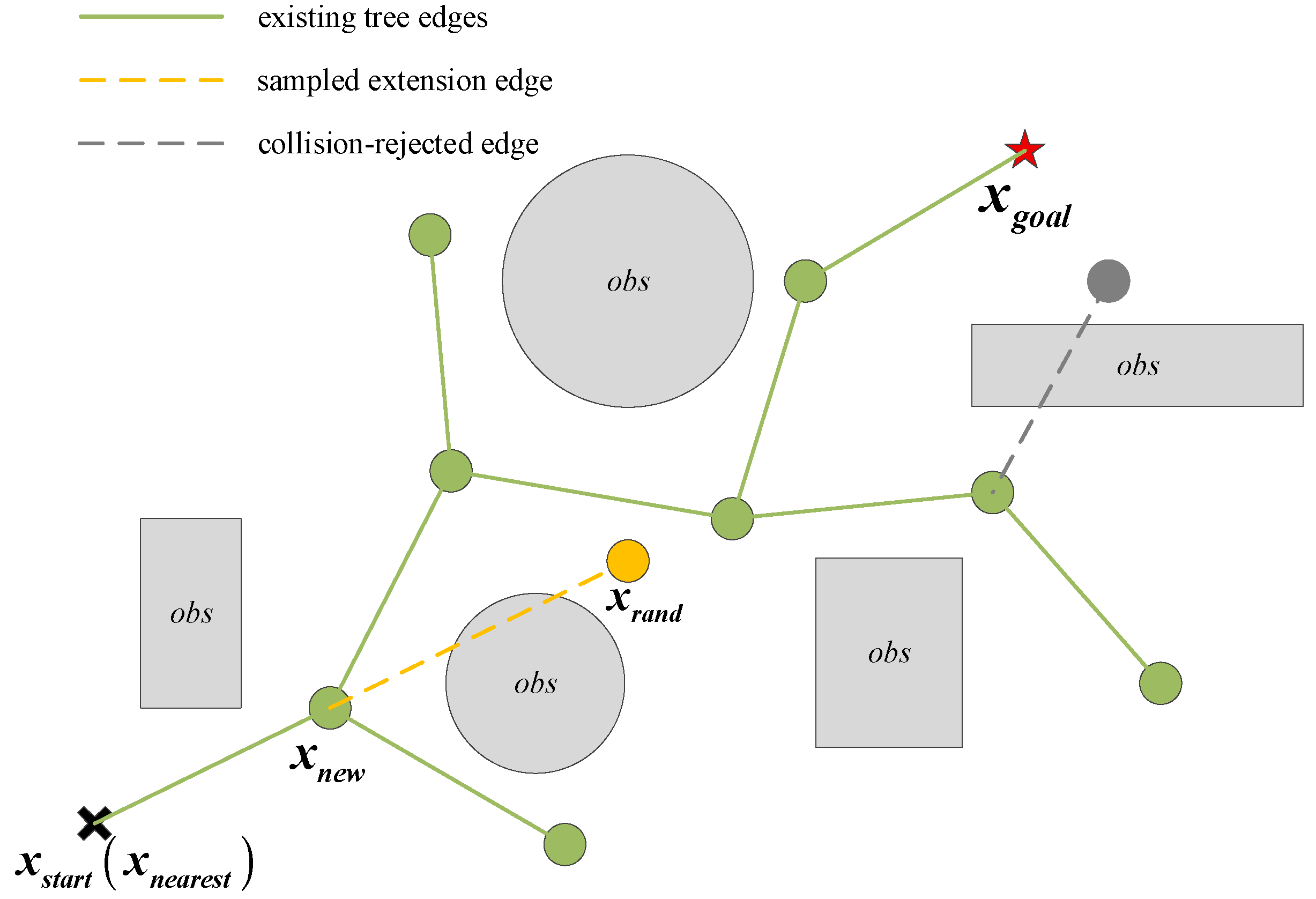
As shown in Figure 1, the tree expands from $x_{\mathrm{start}}$ toward randomly sampled configurations while avoiding obstacle regions. When the extension from $x_{\mathrm{nearest}}$ to $x_{\mathrm{new}}$ is feasible, the new node is inserted into the tree. If the extension intersects an obstacle, the corresponding candidate is discarded. Through repeated sampling and extension, RRT can rapidly explore the free space and find a feasible path to the goal region. The basic RRT procedure is summarized in Algorithm 1.

Figure 1. Schematic illustration of RRT-based node expansion.

Figure 1. Schematic illustration of RRT-based node expansion.

Algorithm 1. RRT.
Input: Xfree, xstart, xgoal, Nmax, step size η.
Output: Search tree T = (V,E) and feasible path σ, if found.
1:	V ← {xstart}, E ← ∅
2:	for i = 1 to Nmax do
3:	xrand ← Sample(Xfree)
4:	xnearest ← Nearest(V, xrand)
5:	xnew ← Steer(xnearest, xrand, η)
6:	if CollisionFree(xnearest, xnew) then
7:	V ← V ∪ {xnew}
8:	E ← E ∪ {(xnearest,xnew)}
9:	if xnew reaches the goal region then
10:	return T = (V, E) and σ
11:	end if
12:	end if
13:	end for
14:	return T = (V, E)

RRT* improves RRT by introducing parent selection and rewiring operations. After a valid node $x_{\mathrm{new}}$ is generated, a set of neighboring nodes $X_{\mathrm{near}}$ is searched around $x_{\mathrm{new}}$. The ChooseParent procedure selects the parent node that gives the lowest accumulated path cost, rather than directly connecting $x_{\mathrm{new}}$ to $x_{\mathrm{nearest}}$. Then, the Rewire procedure checks whether nearby nodes can reduce their path cost by reconnecting through $x_{\mathrm{new}}$. These two operations allow the search tree to be progressively optimized during sampling, thereby improving path quality and accelerating convergence in the search process. The complete RRT* procedure is summarized in Algorithm 2.

Algorithm 2. RRT*.
Input: Xfree, xstart, xgoal, Nmax, step size η, neighborhood radius r.
Output: Search tree T = (V,E) and best path σ*, if found.
1:	V ← {xstart}, E ← ∅, σ* ← ∅
2:	for i = 1 to Nmax do
3:	xrand ← Sample(Xfree)
4:	xnearest ← Nearest(V, xrand)
5:	xnew ← Steer(xnearest, xrand, η)
6:	if CollisionFree(xnearest, xnew) then
7:	Xnear ← Near(V, xnew, r)
8:	xparent ← ChooseParent(Xnear, xnew, xnearest)
9:	V ← V ∪ {xnew}
10:	E ← E ∪ {(xparent,xnew)}
11:	T ← Rewire(T,Xnear,xnew)
12:	if xnew reaches the goal region then
13:	Update the current best path σ*
14:	end if
15:	end if
16:	end for
17:	return T = (V, E) and σ*

2.3. Informed-RRT*

Informed-RRT* improves RRT* by introducing heuristic sampling after an initial feasible path has been obtained. Before the first feasible solution is found, the algorithm samples in the free space in the same manner as RRT*. Once a feasible path exists, the current best path cost $c_{\mathrm{b}\mathrm{e}\mathrm{s}\mathrm{t}}$ is used to define an ellipsoidal subset, and subsequent samples are generated only inside this subset.

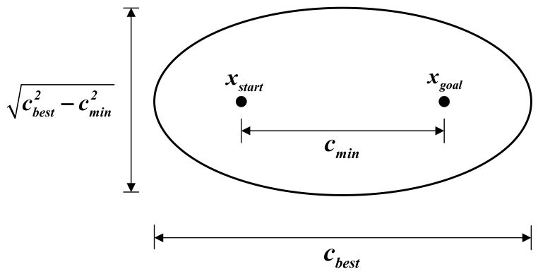
As shown in Figure 2, $x_{\mathrm{s}\mathrm{t}\mathrm{a}\mathrm{r}\mathrm{t}}$ and $x_{\mathrm{g}\mathrm{o}\mathrm{a}\mathrm{l}}$ are the two foci of the ellipse. The Euclidean distance between them is denoted as $c_{\mathrm{m}\mathrm{i}\mathrm{n}}$:

$$c_{\mathrm{m}\mathrm{i}\mathrm{n}}=\parallel x_{\mathrm{g}\mathrm{o}\mathrm{a}\mathrm{l}}-x_{\mathrm{s}\mathrm{t}\mathrm{a}\mathrm{r}\mathrm{t}}{\parallel }_2.$$

(1)

For a candidate sample $x_{\mathrm{r}\mathrm{a}\mathrm{n}\mathrm{d}}$, the path through this sample can improve the current solution only if the sum of its distances to the start and goal configurations is not larger than $c_{\mathrm{b}\mathrm{e}\mathrm{s}\mathrm{t}}$. Therefore, the informed sampling subset is defined as

$$X_{\mathrm{i}\mathrm{n}\mathrm{f}}=\left\{x\in X_{\mathrm{f}\mathrm{r}\mathrm{e}\mathrm{e}}\mid \parallel x-x_{\mathrm{s}\mathrm{t}\mathrm{a}\mathrm{r}\mathrm{t}}{\parallel }_2+\parallel x-x_{\mathrm{g}\mathrm{o}\mathrm{a}\mathrm{l}}{\parallel }_2\le c_{\mathrm{b}\mathrm{e}\mathrm{s}\mathrm{t}}\right\}.$$

(2)

In the two-dimensional case, this subset corresponds to an ellipse whose major-axis length is $c_{\mathrm{b}\mathrm{e}\mathrm{s}\mathrm{t}}$, and the distance between the two foci is $c_{\mathrm{m}\mathrm{i}\mathrm{n}}$. The semi-major axis $a$, half focal distance $c$, and semi-minor axis $b$ are given by

$$a={\displaystyle \frac{c_{\mathrm{b}\mathrm{e}\mathrm{s}\mathrm{t}}}{2}},c={\displaystyle \frac{c_{\mathrm{m}\mathrm{i}\mathrm{n}}}{2}},b={\displaystyle \frac{\sqrt{c_{\mathrm{b}\mathrm{e}\mathrm{s}\mathrm{t}}^2-c_{min}^2}}{2}}.$$

(3)

As $c_{\mathrm{b}\mathrm{e}\mathrm{s}\mathrm{t}}$ decreases during path optimization, the elliptical sampling region gradually shrinks.

Figure 2. Elliptical sampling region of Informed-RRT*.

Figure 2. Elliptical sampling region of Informed-RRT*.

The main procedure of Informed-RRT* is given in Algorithm 3. The algorithm preserves the tree expansion, parent selection, and rewiring operations of RRT*, while replacing global sampling with informed sampling after a feasible solution is available.

Algorithm 3. Informed-RRT*.
Input: Xfree, xstart, xgoal, Nmax, step size η, neighborhood radius r.
Output: Search tree T = (V,E) and best path σ*, if found.
1:	V ← {xstart}, E ← ∅, Σsol ← ∅
2:	cbest ← ∞
3:	for i = 1 to Nmax do
4:	if cbest < ∞ then
5:	xrand ← InformedSample(xstart,xgoal,cbest)
6:	else
7:	xrand ← Sample(Xfree)
8:	end if
9:	xnearest ← Nearest(V, xrand)
10:	xnew ← Steer(xnearest, xrand, η)
11:	if CollisionFree(xnearest, xnew) then
12:	Xnear ← Near(V, xnew, r)
13:	xparent ← ChooseParent(Xnear, xnew, xnearest)
14:	V ← V ∪ {xnew}
15:	E ← E ∪ {(xparent,xnew)}
16:	T ← Rewire(T,Xnear,xnew)
17:	if xnew reaches the goal region then
18:	Σsol ← Σsol ∪ {xnew}
19:	Update cbest and σ*
20:	end if
21:	end if
22:	end for
23:	return T = (V, E) and σ*

3. Proposed RC-Informed-RRT*

3.1. Risk-Density-Aware Corridor Sampling

Informed-RRT* restricts the sampling region after an initial feasible path is obtained, but the samples inside the ellipsoidal subset are still generated without explicitly considering obstacle distribution. As a result, some samples may be located close to obstacles or in locally cluttered regions, leading to ineffective expansion and unnecessary collision checking. To reduce such low-contribution sampling, RC-Informed-RRT* introduces a risk-density-aware corridor sampling mechanism. The mechanism constructs a soft corridor around a reference path and evaluates candidate samples by combining corridor deviation, obstacle clearance, and local obstacle density.

The sampling domain is determined by the current planning state:

$$X_s=\{\begin{array}{ll}{X}_{\mathrm{f}\mathrm{r}\mathrm{e}\mathrm{e}},& c_{\mathrm{b}\mathrm{e}\mathrm{s}\mathrm{t}}=\mathrm{\infty }\\ X_{\mathrm{i}\mathrm{n}\mathrm{f}},& c_{\mathrm{b}\mathrm{e}\mathrm{s}\mathrm{t}}<\mathrm{\infty }\end{array},$$

(4)

where $c_{\mathrm{b}\mathrm{e}\mathrm{s}\mathrm{t}}$ is the cost of the current best path, and $X_{\mathrm{i}\mathrm{n}\mathrm{f}}$ denotes the informed sampling subset. Before the first feasible path is obtained, the straight line connecting $x_{\mathrm{s}\mathrm{t}\mathrm{a}\mathrm{r}\mathrm{t}}$ and $x_{\mathrm{g}\mathrm{o}\mathrm{a}\mathrm{l}}$ is used as the reference path $\Gamma$. After a feasible path is found, the current best path ${\sigma }_{\mathrm{b}\mathrm{e}\mathrm{s}\mathrm{t}}$ is used as $\Gamma$. For a candidate sample $x$, its distance to the reference corridor is defined as:

$$d_c\left(x\right)=\underset{y\in \Gamma }{\mathrm{m}\mathrm{i}\mathrm{n} }{\parallel x-y\parallel }_2.$$

(5)

Here, $d_c\left(x\right)$ represents the shortest Euclidean distance from the candidate sample $x$ to the reference path $\Gamma$. This distance is used to measure whether the sample lies near the currently preferred search corridor.

The risk-density value of $x$ is defined by combining obstacle clearance and the number of nearby obstacles:

$$\rho \left(x\right)=\mathrm{c}\mathrm{l}\mathrm{i}\mathrm{p}\left(w_1{e}^{-d_{\mathrm{o}\mathrm{b}\mathrm{s}}\left(x\right)/\lambda }+w_2{\displaystyle \frac{n_{\mathrm{o}\mathrm{b}\mathrm{s}}\left(x,r_d\right)}{n_{\mathrm{m}\mathrm{a}\mathrm{x}}}},\mathrm{0,1}\right),$$

(6)

where $d_{obs}\left(x\right) = {\min }_k d(x, O_k)$ is the minimum Euclidean distance from $x$ to the obstacle set, and $n_{obs}$($x$, $r_d$) = |{$O_k$: $d$($x$, $O_k$) ≤ $r_d$}| is the number of distinct obstacle primitives whose distance from $x$ does not exceed the local radius $r_d$. Obstacle size and shape therefore affect both the minimum clearance and the number of obstacle regions intersecting the local neighborhood. The four evaluated maps contain non-overlapping rectangular and circular obstacle primitives, so no overlap correction is required in the present experiments. For general inputs containing overlapping primitives, their occupied regions should first be merged geometrically to avoid duplicate counting. A larger $\rho \left(x\right)$ indicates either smaller obstacle clearance or a larger number of nearby obstacle regions.

The local corridor radius is adjusted according to the risk-density value:

$$r_c\left(x,i\right)=r_0\chi \left(i\right)\left(1+\beta \rho \left(x\right)\right),$$

(7)

where r₀ is the base corridor radius and β controls the local widening effect. Before the first feasible solution is obtained, the refinement factor is set to χ(i) = χ_pre. After the first feasible solution, χ(i) decreases linearly from χ_post,start to χ_post,end according to the normalized post-solution progress clip ((i − i_first)/(N_max − i_first), 0, 1). In the reported experiments, χ_pre = 1.55, χ_post,start = 1.20, and χ_post,end = 0.65. Thus, 1 + βρ(x) locally widens the corridor in cluttered regions, while the stage-dependent factor progressively tightens the corridor after a feasible solution becomes available without reducing its width to zero.

If $d_c\left(x\right)>\kappa r_c\left(x,i\right)$, the candidate sample is directly rejected because it is too far from the reference corridor. Otherwise, it is accepted according to the following probability:

$$P_{\mathrm{a}\mathrm{c}\mathrm{c}}\left(x\right)=\mathrm{m}\mathrm{a}\mathrm{x}\left(P_{\mathrm{m}\mathrm{i}\mathrm{n}},\mathrm{e}\mathrm{x}\mathrm{p}\left[-\alpha {\left({\displaystyle \frac{d_c\left(x\right)}{r_c\left(x,i\right)}}\right)}^2-\gamma \rho \left(x\right)\right]\right),$$

(8)

where $\kappa$ is the hard rejection coefficient, $\alpha$ and $\gamma$ control the effects of corridor deviation and risk density, respectively, and $P_{\mathrm{m}\mathrm{i}\mathrm{n}}$ is the minimum acceptance probability used to prevent the sampling process from becoming overly restrictive. If no sample is accepted after $N_r$ trials, a fallback sample is drawn from $X_s$. This fallback strategy preserves exploration diversity and reduces the risk of prematurely excluding feasible detour regions. The complete sampling procedure is summarized in Algorithm 4.

Algorithm 4. RiskCorridorSample.
Input: Xfree, Xinf, Xobs, cbest, σbest, xstart, xgoal, i, Nr.
Output: xrand.
1:	Xs ← SelectSpace(Xfree,Xinf,cbest);
2:	Γ ← ReferencePath(xstart,xgoal,σbest,cbest);
3:	for j = 1 to Nr do
4:	x ← Sample(Xs);
5:	dc ← CorridorDistance(x,Γ);
6:	ρ ← RiskDensity(x,Xobs);
7:	rc ← CorridorRadius(ρ,i);
8:	if dc > κrc then
9:	continue;
10:	end if
11:	Pacc ← AcceptRate(dc,rc,ρ);
12:	if Random(0,1) < Pacc then
13:	xrand ← x;
14:	return xrand;
15:	end if
16:	end for
17:	xrand ← Sample(Xs);
18:	return xrand;

3.2. Improvement-Bound Rejection

Although the risk-density-aware corridor sampling mechanism improves the spatial distribution of candidate samples, some generated nodes may still have limited potential to reduce the current path cost. In RRT*-based algorithms, each inserted node may trigger parent selection and rewiring operations. Therefore, after an initial feasible path is obtained, RC-Informed-RRT* rejects low-contribution nodes before tree insertion.

For a newly generated node $x_{\mathrm{n}\mathrm{e}\mathrm{w}}$, let $x_{\mathrm{p}\mathrm{a}\mathrm{r}\mathrm{e}\mathrm{n}\mathrm{t}}$ be its parent node and $g_{\mathrm{p}\mathrm{a}\mathrm{r}\mathrm{e}\mathrm{n}\mathrm{t}}$ be the accumulated path cost from $x_{\mathrm{s}\mathrm{t}\mathrm{a}\mathrm{r}\mathrm{t}}$ to $x_{\mathrm{p}\mathrm{a}\mathrm{r}\mathrm{e}\mathrm{n}\mathrm{t}}$. The optimistic cost of a path passing through $x_{\mathrm{n}\mathrm{e}\mathrm{w}}$ is defined as

$$c_{\mathrm{l}\mathrm{b}}(x_{\mathrm{n}\mathrm{e}\mathrm{w}})=g_{\mathrm{p}\mathrm{a}\mathrm{r}\mathrm{e}\mathrm{n}\mathrm{t}}+\parallel x_{\mathrm{n}\mathrm{e}\mathrm{w}}-x_{\mathrm{p}\mathrm{a}\mathrm{r}\mathrm{e}\mathrm{n}\mathrm{t}}\parallel +\parallel x_{\mathrm{g}\mathrm{o}\mathrm{a}\mathrm{l}}-x_{\mathrm{n}\mathrm{e}\mathrm{w}}\parallel .$$

(9)

The last term only uses the Euclidean distance from $x_{\mathrm{n}\mathrm{e}\mathrm{w}}$ to $x_{\mathrm{g}\mathrm{o}\mathrm{a}\mathrm{l}}$, without considering obstacles or detours. Thus, $c_{\mathrm{l}\mathrm{b}}\left(x_{\mathrm{n}\mathrm{e}\mathrm{w}}\right)$ gives an optimistic lower-bound estimate of the path cost through $x_{\mathrm{n}\mathrm{e}\mathrm{w}}$. The potential improvement margin is then given by

$$\mathsf{\Delta }c\left(x_{\mathrm{n}\mathrm{e}\mathrm{w}}\right)=c_{\mathrm{b}\mathrm{e}\mathrm{s}\mathrm{t}}-c_{\mathrm{l}\mathrm{b}}\left(x_{\mathrm{n}\mathrm{e}\mathrm{w}}\right),$$

(10)

where $c_{\mathrm{b}\mathrm{e}\mathrm{s}\mathrm{t}}$ is the current best path cost. A larger $\mathsf{\Delta }c\left(x_{\mathrm{n}\mathrm{e}\mathrm{w}}\right)$ indicates that the candidate node has greater potential to improve the current solution.

To avoid excessive rejection in obstacle-dense regions, the rejection threshold is adjusted by the local risk-density value. The risk density of $x_{\mathrm{n}\mathrm{e}\mathrm{w}}$ follows the definition in Section 3.1:

$$\rho (x_{\mathrm{n}\mathrm{e}\mathrm{w}})=\mathrm{c}\mathrm{l}\mathrm{i}\mathrm{p}\left(w_1{e}^{-d_{\mathrm{o}\mathrm{b}\mathrm{s}}\left(x_{\mathrm{n}\mathrm{e}\mathrm{w}}\right)/\lambda }+w_2{\displaystyle \frac{n_{\mathrm{o}\mathrm{b}\mathrm{s}}(x_{\mathrm{n}\mathrm{e}\mathrm{w}},r_d)}{n_{\mathrm{m}\mathrm{a}\mathrm{x}}}},\mathrm{0,1}\right).$$

(11)

The optimization progress after the first feasible path is defined as

$$s(i)={\displaystyle \frac{i-i_{\mathrm{f}\mathrm{i}\mathrm{r}\mathrm{s}\mathrm{t}}}{N_{\mathrm{m}\mathrm{a}\mathrm{x}}-i_{\mathrm{f}\mathrm{i}\mathrm{r}\mathrm{s}\mathrm{t}}}},$$

(12)

where $i_{\mathrm{f}\mathrm{i}\mathrm{r}\mathrm{s}\mathrm{t}}$ is the iteration index at which the first feasible path is obtained, and $N_{\mathrm{m}\mathrm{a}\mathrm{x}}$ is the maximum number of iterations. The stage-dependent scale factor is

$$\mu (i)={\mu }_{\mathrm{m}\mathrm{i}\mathrm{n}}+({\mu }_{\mathrm{m}\mathrm{a}\mathrm{x}}-{\mu }_{\mathrm{m}\mathrm{i}\mathrm{n}})s(i),$$

(13)

where ${\mu }_{\mathrm{m}\mathrm{i}\mathrm{n}}$ and ${\mu }_{\mathrm{m}\mathrm{a}\mathrm{x}}$ control the lower and upper bounds of the rejection strength. The final rejection threshold is defined as

$$\epsilon (x_{\mathrm{n}\mathrm{e}\mathrm{w}},i)={\epsilon }_0\mu \left(i\right)\mathrm{m}\mathrm{a}\mathrm{x}(1-\xi \rho (x_{\mathrm{n}\mathrm{e}\mathrm{w}}),\delta ),$$

(14)

where ${\epsilon }_0$ is the base threshold, $\xi$ controls the relaxation degree in high-risk regions, and $\delta$ prevents the threshold from becoming too small. When $\rho \left(x_{\mathrm{n}\mathrm{e}\mathrm{w}}\right)$ is large, the threshold decreases, allowing more detour-related nodes to be retained in cluttered regions.

The rejection condition is defined as

$$\mathsf{\Delta }c\left(x_{\mathrm{n}\mathrm{e}\mathrm{w}}\right)<\epsilon (x_{\mathrm{n}\mathrm{e}\mathrm{w}},i).$$

(15)

If the above condition is satisfied, $x_{\mathrm{n}\mathrm{e}\mathrm{w}}$ is rejected after provisional parent selection and before final node insertion and rewiring. Otherwise, it is inserted into the tree for subsequent optimization.

The rejection rule is intended as a finite-horizon efficiency–accuracy trade-off. Because $c_{lb}$ is an optimistic lower bound, $\Delta c<\epsilon$ indicates that the candidate cannot improve the incumbent solution by at least the current threshold even under an optimistic continuation. A positive $\epsilon$ may discard improvements satisfying $0<\Delta c<\epsilon$; therefore, strict asymptotic optimality is not claimed for the thresholded variant. The rule is used to reduce low-contribution node insertion and rewiring under the fixed iteration budget adopted in this study.

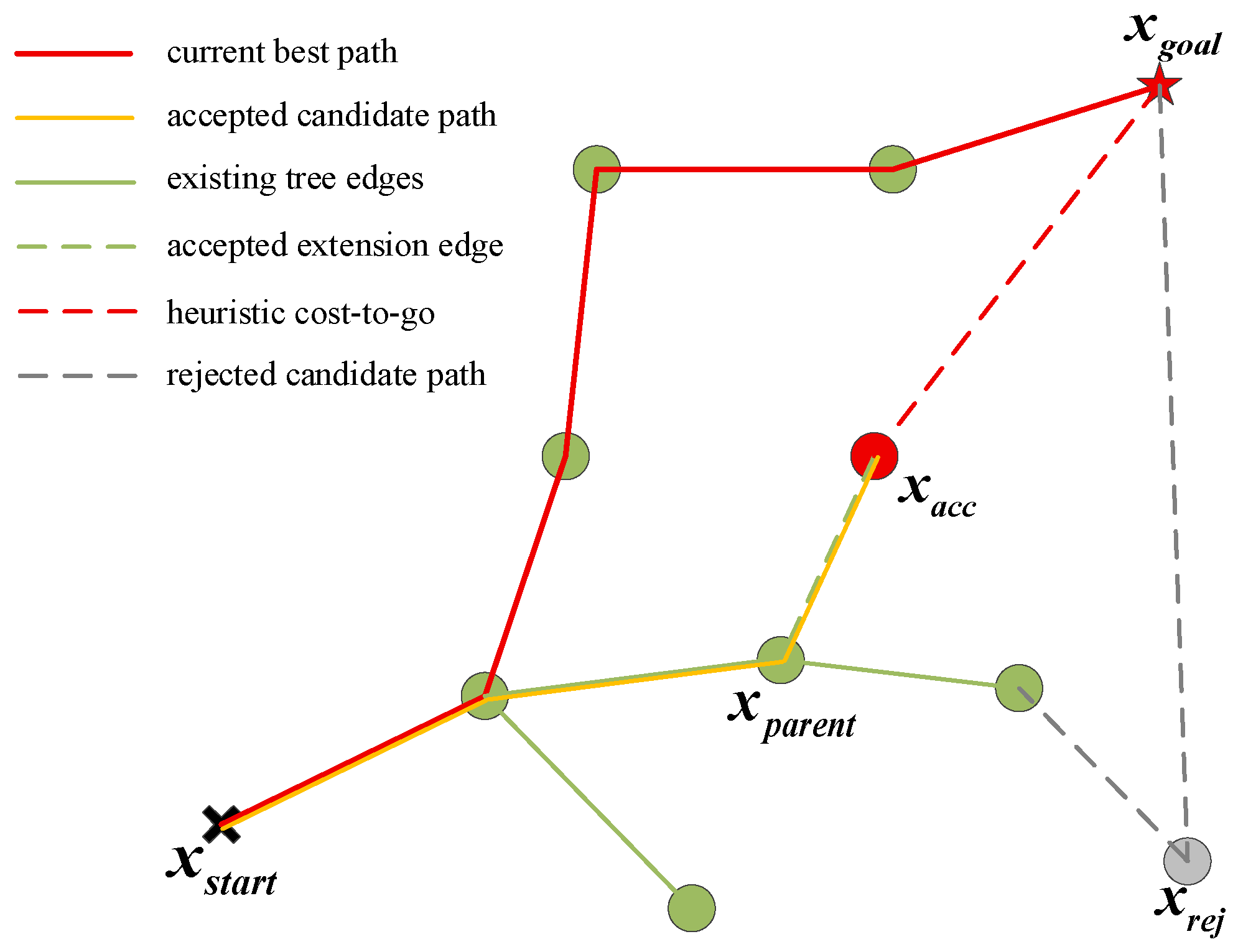
Figure 3 illustrates the improvement-bound rejection mechanism after provisional parent selection. In this mechanism, a candidate node $x_{\mathrm{n}\mathrm{e}\mathrm{w}}$ is accepted only when its optimistic path cost still provides sufficient improvement potential with respect to the current best path; otherwise, it is rejected before node insertion and rewiring.

The corresponding improvement-bound rejection procedure is summarized in Algorithm 5. The algorithm is inactive before the first feasible path is obtained; after a provisional parent $x_{\mathrm{p}\mathrm{a}\mathrm{r}\mathrm{e}\mathrm{n}\mathrm{t}}$ has been selected, it computes the optimistic improvement margin and rejects a candidate node only when the margin is smaller than the adaptive threshold.

Algorithm 5. ImprovementBoundReject.
Input: xnew, xparent, gparent, xgoal, cbest, Xobs, i, ifirst, Nmax.
Output: brej.
1:	if cbest = ∞ then
2:	brej ← False;
3:	return brej;
4:	end if
5:	dobs ← minz∈Xobs ‖xnew − z‖;
6:	nobs ← |{Ok ∈ Xobs: d(xnew,Ok) ≤ rd}|;
7:	ρ ← clip(w1e−dobs/λ + w2nobs/nmax,0,1);
8:	clb ← gparent + ‖xnew − xparent‖ + ‖xgoal − xnew‖;
9:	Δc ← cbest − clb;
10:	s(i) ← (i − ifirst)/(Nmax − ifirst);
11:	μ(i) ← μmin + (μmax − μmin)s(i);
12:	ε ← ε0μ(i)max(1 − ξρ,δ);
13:	if Δc < ε then
14:	brej ← True;
15:	else
16:	brej ← False;
17:	end if
18:	return brej;

3.3. Search-State-Regulated Goal Bias

A fixed goal-bias probability can accelerate tree expansion toward the goal, but an excessively large value may reduce exploration diversity, especially in obstacle-dense environments. Conversely, a small value may delay the generation of the first feasible path. Therefore, RC-Informed-RRT* adopts a search-state-regulated goal-bias strategy, in which the goal sampling probability is adjusted according to the current search state.

At each iteration, the search state is described by three factors: the tree-to-goal distance, the stagnation degree, and the planning phase. The normalized tree-to-goal distance is defined as

$$d_g(i)=\mathrm{m}\mathrm{i}\mathrm{n}({\displaystyle \frac{\underset{x\in V_i}{\mathrm{m}\mathrm{i}\mathrm{n}}\parallel x-x_{\mathrm{g}\mathrm{o}\mathrm{a}\mathrm{l}}\parallel }{\parallel x_{\mathrm{s}\mathrm{t}\mathrm{a}\mathrm{r}\mathrm{t}}-x_{\mathrm{g}\mathrm{o}\mathrm{a}\mathrm{l}}\parallel }},1),$$

(16)

where $V_i$ is the node set at iteration $i$. A smaller $d_g\left(i\right)$ indicates that the tree has expanded closer to the goal region.

The stagnation degree is described by the number of iterations since the last effective progress:

$$\tau (i)=\mathrm{m}\mathrm{i}\mathrm{n}({\displaystyle \frac{i-i_p}{W_s}},1),$$

(17)

where $i_p$ records the latest iteration in which the search makes effective progress, and $W_s$ is the stagnation window. Before the first feasible path is obtained, effective progress means that the minimum distance from the tree to the goal decreases. After a feasible path is found, effective progress means that $c_{\mathrm{b}\mathrm{e}\mathrm{s}\mathrm{t}}$ is improved.

The phase factor is defined as

$$\varphi (i)=\{\begin{array}{cc}1,& c_{\mathrm{b}\mathrm{e}\mathrm{s}\mathrm{t}}=\mathrm{\infty }\\ {\varphi }_{\mathrm{o}\mathrm{p}\mathrm{t}},& c_{\mathrm{b}\mathrm{e}\mathrm{s}\mathrm{t}}<\mathrm{\infty }\end{array},$$

(18)

where $0<{\varphi }_{\mathrm{o}\mathrm{p}\mathrm{t}}<1$. This setting keeps a stronger goal-oriented tendency before the first feasible path is found and reduces the goal bias during the optimization stage.

The search-state score is calculated as

$$S_g(i)=\mathrm{m}\mathrm{i}\mathrm{n}\left(\mathrm{m}\mathrm{a}\mathrm{x}\left({\omega }_d(1-d_g(i))+{\omega }_s(1-\tau (i))+{\omega }_{\varphi }\varphi (i),0\right),1\right),$$

(19)

where ${\omega }_d$, ${\omega }_s$, and ${\omega }_{\varphi }$ are weighting coefficients. The goal-bias probability is then bounded by

$$p_{\mathrm{g}\mathrm{o}\mathrm{a}\mathrm{l}}(i)=p_{\mathrm{m}\mathrm{i}\mathrm{n}}+(p_{\mathrm{m}\mathrm{a}\mathrm{x}}-p_{\mathrm{m}\mathrm{i}\mathrm{n}})S_g(i),$$

(20)

where $p_{\mathrm{m}\mathrm{i}\mathrm{n}}$ and $p_{\mathrm{m}\mathrm{a}\mathrm{x}}$ are the lower and upper bounds of the goal-bias probability. When the tree approaches the goal and the search is not stagnant, $p_{\mathrm{g}\mathrm{o}\mathrm{a}\mathrm{l}}$ increases to promote fast connection. When the search becomes stagnant, $p_{\mathrm{g}\mathrm{o}\mathrm{a}\mathrm{l}}$ decreases to preserve random exploration.

For reproducibility, the implementation uses phase-specific bounded coefficients. Before the first feasible solution, the goal-bias probability is limited to [0.04, 0.28] and combines goal closeness, stagnation, and an early-stage term with coefficients 0.14, 0.10, and 0.08, respectively. After the first feasible solution, the probability is limited to [0.03, 0.22] and uses coefficients 0.05, 0.09, and 0.04 for goal closeness, stagnation, and post-solution progress. The stagnation normalization window is 220 iterations, and these coefficients are fixed in all reported experiments.

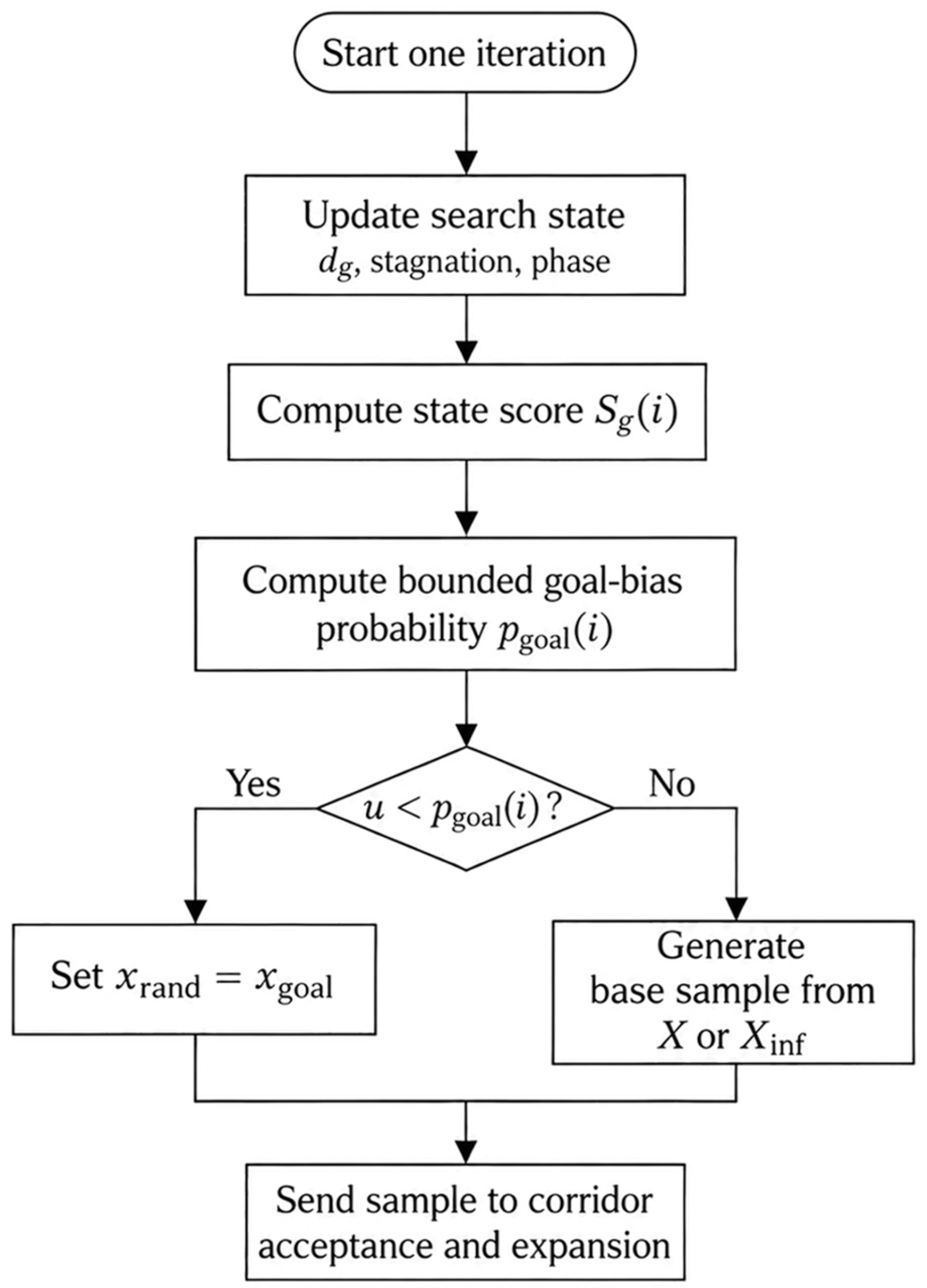
Figure 4 shows the workflow of the search-state-regulated goal-bias strategy, and Algorithm 6 summarizes the corresponding pseudocode. The search state is updated at the beginning of each iteration, and the resulting goal-bias probability determines whether the current sample is set to $x_{\mathrm{g}\mathrm{o}\mathrm{a}\mathrm{l}}$ or generated from the basic sampling domain.

Figure 4. Search-state-regulated goal-bias strategy.

Figure 4. Search-state-regulated goal-bias strategy.

Algorithm 6. StateRegulatedGoalBias.
Input: Vi, Xs, xstart, xgoal, cbest, i, ip, Ws.
Output: xrand, bgoal.
1:	dg ← min (minx∈Vi ‖x − xgoal‖/‖xstart − xgoal‖,1);
2:	τ ← min ((i − ip)/Ws,1);
3:	if cbest = ∞ then
4:	ϕ ← 1;
5:	else
6:	ϕ ← ϕopt;
7:	end if
8:	Sg ← min (max (ωd(1 − dg) + ωs(1 − τ) + ωϕϕ,0),1);
9:	pgoal ← pmin + (pmax − pmin)Sg;
10:	u ← Random(0,1);
11:	if u < pgoal then
12:	xrand ← xgoal;
13:	bgoal ← True;
14:	else
15:	xrand ← Sample(Xs);
16:	bgoal ← False;
17:	end if
18:	return xrand, bgoal;

The complete RC-Informed-RRT* planning procedure, which integrates the three modules described in Algorithms 4–6, is summarized in Algorithm 7.

Algorithm 7. RC-Informed-RRT*.
Input: Xfree, Xobs, xstart, xgoal, Nmax, step size η, neighborhood radius r, Nr, Ws, dtol.
Output: Search tree T = (V,E) and best path σbest, if found.
1:	V ← {xstart}, E ← ∅, σbest ← ∅;
2:	cbest ← ∞, ifirst ← ∞, ip ← 0;
3:	for i = 1 to Nmax do
4:	Xinf ← InformedSubset(xstart,xgoal,cbest);
5:	Xs ← SelectSpace(Xfree,Xinf,cbest);
6:	(xrand,bgoal) ← StateRegulatedGoalBias(V,Xs,xstart,xgoal,cbest,i,ip,Ws);
7:	if bgoal = False then
8:	xrand ← RiskCorridorSample(Xfree,Xinf,Xobs,cbest,σbest,xstart,xgoal,i,Nr);
9:	end if
10:	xnearest ← Nearest(V,xrand);
11:	xnew ← Steer(xnearest,xrand,η);
12:	if CollisionFree(xnearest,xnew) then
13:	Xnear ← Near(V,xnew,r);
14:	xparent ← ChooseParent(Xnear,xnew,xnearest);
15:	gparent ← Cost(xparent);
16:	brej ← ImprovementBoundReject(xnew,xparent,gparent,xgoal,cbest,Xobs,i,ifirst,Nmax);
17:	if brej = False then
18:	V ← V ∪ {xnew};
19:	E ← E ∪ {(xparent,xnew)};
20:	T ← Rewire(T,Xnear,xnew);
21:	(cbest,σbest,ifirst,ip) ← UpdateBestAndState(T,xnew,xgoal,dtol,i);
22:	end if
23:	end if
24:	end for
25:	return T = (V,E) and σbest;

In Algorithm 7, UpdateBestAndState records i_first when the first feasible path is obtained, updates i_p whenever effective progress occurs, and updates c_best and σ_best whenever a lower-cost solution is found.

3.4. Algorithm Analysis

As summarized in Algorithm 7, RC-Informed-RRT* retains the basic expansion, parent-selection, and rewiring structure of Informed-RRT*. The proposed improvements mainly act before node insertion. The search-state-regulated goal bias adjusts the sampling direction at the beginning of each iteration. The risk-density-aware corridor sampling improves the spatial quality of non-goal samples. The improvement-bound rejection further filters low-contribution nodes after provisional parent selection and before final node insertion and rewiring.

Compared with Informed-RRT*, RC-Informed-RRT* provides more targeted exploration in different planning stages. Before the first feasible path is found, the adaptive goal bias helps the tree approach the goal more efficiently while retaining random exploration. After a feasible path is obtained, the corridor mechanism distinguishes samples inside the informed subset according to corridor distance, obstacle clearance, and local obstacle density. Therefore, samples near safer and more promising regions are more likely to be selected. The rejection mechanism then reduces redundant nodes whose optimistic cost is unlikely to improve the current best path.

These mechanisms do not deterministically eliminate exploration. The improvement-bound rejection is inactive before the first feasible solution is obtained, and corridor sampling retains both a minimum acceptance probability and fallback sampling. Consequently, the planner preserves nonzero opportunities for exploratory sampling outside the preferred corridor during finite runs, including in detour-dominated regions.

Let n denote the current number of tree nodes, M the number of obstacle primitives, N_r the maximum number of candidate trials in corridor sampling, and k = |X_near| the number of nodes returned by the neighborhood query. With the direct linear searches used in the implementation, nearest-neighbor and near-neighbor queries require O(n) work, while a direct collision or risk-density evaluation scales with O(M). Corridor sampling evaluates at most N_r candidates and therefore contributes O(N_r M) obstacle-processing work per iteration. Parent selection and rewiring inspect at most k neighboring nodes; when a candidate reconnection requires direct collision validation, these operations contribute at most O(k M) work. In the current implementation, a successful rewire also refreshes the accumulated costs of the affected descendant subtree. If q descendant-node visits are triggered by successful rewiring in one iteration, the linear parent-array scan used to identify children adds O(q n) work. Hence, an implementation-level per-iteration bound is O(n + (N_r + k)M + qn). The storage requirement remains O(n + M). This expression makes the rewiring contribution explicit: k controls the neighborhood-level collision checks, whereas q captures the additional descendant-cost propagation caused by successful rewires. In typical local neighborhoods, both the returned neighborhood and affected descendant sets are substantially smaller than the full tree; spatial indexing and child-adjacency structures can further reduce these terms in larger implementations.

4. Simulation Results

To evaluate RC-Informed-RRT*, comparative simulations were conducted with RRT, RRT*, and Informed-RRT* in four two-dimensional static environments. All algorithms were implemented in MATLAB R2024b (The MathWorks, Inc., Natick, MA, USA) and executed on Windows 11 (64-bit) using a 13th Gen Intel(R) Core(TM) i7-13620H CPU (Intel Corporation, Santa Clara, CA, USA) at 2.40 GHz and 32 GB of RAM. Because sampling-based planners are stochastic, each algorithm was evaluated in 50 independent trials per environment. The trial count was increased to reduce sampling variability, while the per-trial iteration budgets and collision-checking conditions remained unchanged. The reported results evaluate planning efficiency, path quality, smoothness, tree-growth redundancy, and reliability. Additional validation in Section 4.8 includes a sequential ablation study and a fixed goal-bias sensitivity analysis.

RRT, RRT*, and Informed-RRT* are retained as controlled structural baselines because they form the direct algorithmic lineage from which the proposed method is developed. This setting isolates the effect of informed sampling and the three added mechanisms without introducing unrelated modules such as external potential fields, dual-tree coordination, or local trajectory controllers. Recent improved Informed-RRT* variants are instead discussed in Section 1 to clarify methodological differences.

4.1. Map Settings

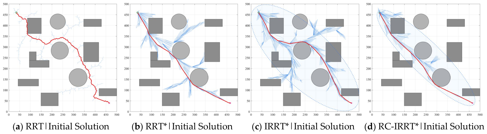
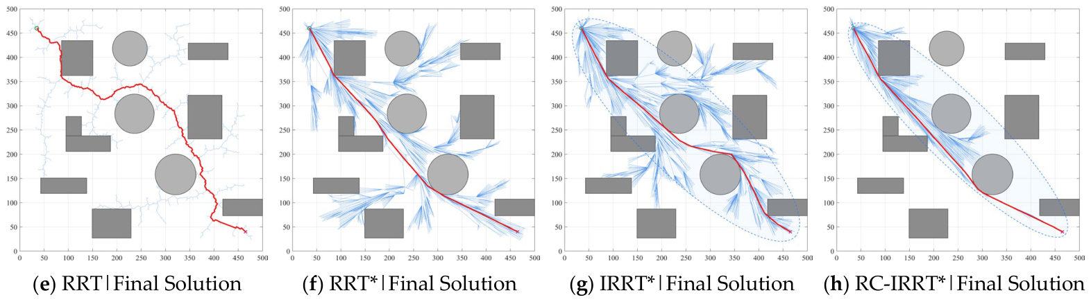
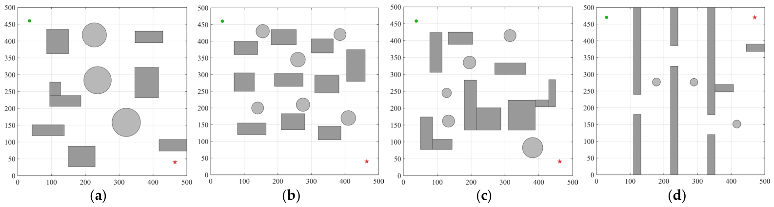
Four representative nominal maps were designed in a 500 × 500 two-dimensional workspace, as shown in Figure 5. To avoid evaluating only one exactly fixed geometric instance, each Monte Carlo trial applies small independent coordinate perturbations around the nominal layout: the start and goal are shifted by uniform x- and y-offsets in [−2, 2] map units, and each static obstacle primitive is translated by uniform x- and y-offsets in [−1, 1] map units without changing its size or shape. Perturbations that would place the start/goal outside the free workspace are resampled. Within a matched trial, the same perturbed environment is used for all compared algorithms. Thus, Figure 5 represents the nominal map geometry, while the statistical results include small local variations in the planning instance.

The sparse environment contains a relatively small number of obstacles and sufficient free space, and it is used to evaluate basic search efficiency and path optimization ability. The dense environment contains more obstacles in a more compact distribution and is used to test the ability of the planner to reduce invalid expansion in cluttered spaces. The narrow-passage environment contains locally constrained regions and limited passages, and it is designed to evaluate the robustness of the algorithm in constrained search spaces. The W-shaped environment is a detour-dominated case in which the feasible route deviates significantly from the direct start-to-goal direction. This map is therefore used to test whether RC-Informed-RRT* can preserve sufficient exploration capability even when the corridor prior is not naturally aligned with the final feasible path.

4.2. Parameters

The main parameters used in the simulations are listed in

Table 1. Main parameters used in the simulations.

Parameter	Description	Value
Workspace size	Map size	500 × 500
Repeated runs	Independent runs for each algorithm in each map	50
Start/goal perturbation	Uniform per-coordinate offset in each trial	[−2, 2]
Obstacle translation perturbation	Uniform x/y translation of each obstacle primitive	[−1, 1]
η	Step size	3
dtol	Goal threshold	10
r	Neighbor radius for parent selection and rewiring	50
Nmax	Maximum iteration number	2300/2300/4500/10,000 for maps (a)–(d)
r0	Base corridor radius	50
α	Corridor-distance weight	1.15
γ	Risk-density weight	0.90
ε0	Basic improvement-bound threshold	6
pg	Fixed goal-bias probability for baseline algorithms	0.08
pgoal(i) range	Adaptive goal-bias probability for RC-Informed-RRT*	[0.03, 0.28]
Pre-solution corridor gate	Probabilistic corridor regulation before the first feasible solution	Enabled by default in RC-Informed-RRT*

Note: Auxiliary coefficients omitted from Table 1 for readability are listed here for reproducibility. Unless otherwise specified, they were fixed across the four environments after preliminary calibration. The risk-density parameters were w1 = 0.60, w2 = 0.40, rd = 45, λ = 15, and nmax = 8. The corridor-sampling parameters were r0 = 50, χpre = 1.55, χpost,start = 1.20, χpost,end = 0.65, β = 0.70, κ = 2.20, α = 1.15, γ = 0.90, Pmin = 0.20 before the first feasible solution and 0.08 afterward, and Nr = 14. The rejection parameters were ε0 = 6, μmin = 0.20, μmax = 1.00, ξ = 0.75, and δ = 0.08. For adaptive goal bias, the pre-solution probability is bounded to [0.04, 0.28], the post-solution probability to [0.03, 0.22], and the stagnation window Ws = 220; the phase-specific coefficients are given in Section 3.3. The overall attainable adaptive range is therefore [0.03, 0.28].

. The same step size, goal threshold, collision-checking condition, termination criterion, and per-trial geometric perturbation protocol were used for all algorithms within each map. The neighbor radius was shared by RRT*, Informed-RRT*, and RC-Informed-RRT*. RC-Informed-RRT* parameters were selected through preliminary calibration to obtain stable behavior and a practical balance between guidance, exploration, and computational efficiency; after calibration, they were kept fixed across the reported trials unless otherwise stated. The fixed goal-bias probability used by the baseline planners was set to 0.08 according to the sensitivity analysis in Section 4.8.2. For readability, Table 1 lists the common comparison settings and principal mechanism-level parameters, while secondary implementation coefficients are reported in the note below the table. Accordingly, the fixed baseline setting p_g = 0.08 is treated as a single shared comparison parameter rather than being retuned for individual baseline planners or maps.

4.3. Evaluation Metrics

To quantitatively evaluate the performance of the four algorithms, six evaluation metrics were used in the simulations, as listed in

Table 2. Evaluation metrics used in the simulations.

Symbol	Metric	Description
$T_p$	Planning time	Computation time required to complete planning; calculated over all trials, including failed trials
$L_i$	Initial path length	Length of the first feasible path found by the algorithm; calculated from successful trials only
$L_f$	Final path length	Length of the best path after all iterations; calculated from successful trials only
$\overline{\theta }$	Mean turn angle	Average turning angle along the final path; calculated from successful trials only
$N_f$	Final node count	Number of nodes retained in the final search tree; calculated over all trials, including failed trials
$S_r$	Success rate	Ratio of successful runs among all 50 independent trials

. These metrics include five continuous metrics, namely $T_p$, $L_i$, $L_f$, $\overline{\theta }$, and $N_f$, and one reliability metric, namely $S_r$. The five continuous metrics are used for distribution-based comparisons in the box plots, whereas the success rate $S_r$ is reported in the corresponding quantitative tables. Planning time $T_p$ was used to evaluate computational efficiency. Initial path length $L_i$ and final path length $L_f$ were used to measure the quality of the first feasible path and the optimized path, respectively. Mean turn angle $\overline{\theta }$ was used to describe path smoothness.

For a path represented by the ordered node sequence $\{x_0, x_1, \dots , x_m\}$, the mean turn angle is defined as

$$\overline{\theta }={\displaystyle \frac{1}{m-1}}{\displaystyle \sum _{i=1}^{m-1}}{\cos }^{-1}({\displaystyle \frac{{(x_i-x_{i-1})}^T(x_{i+1}-x_i)}{{\Vert x_i-x_{i-1}\Vert }_2{\Vert x_{i+1}-x_i\Vert }_2}}).$$

(21)

A smaller $\overline{\theta }$ indicates a smaller average directional change along the polyline. In this paper, smoothness refers only to this geometric turning measure and does not imply satisfaction of curvature, nonholonomic, or kinodynamic constraints. Although averaging reduces the direct influence of the number of internal nodes, the result may still depend on node spacing; therefore, comparisons are made under identical step-size and termination settings.

Final node count $N_f$ was used to evaluate tree-growth redundancy. Success rate $S_r$ was used to measure planning reliability under repeated stochastic trials.

The statistical aggregation rule depends on whether a metric remains well defined when a trial fails. Planning time and final node count are defined for every trial and are therefore calculated over all 50 independent trials, including unsuccessful runs. In a failed trial, the planner proceeds to the prescribed iteration limit, and its measured computation time and terminal tree size are retained in the reported statistics. By contrast, initial path length, final path length, and mean turn angle are calculated only from successful runs because a failed trial does not produce a valid path from which these quantities can be evaluated. The success rate is computed over all 50 trials and is reported together with the corresponding success count. No artificial penalty value is assigned to unavailable path-dependent metrics. This metric-specific treatment retains the computational cost of failed searches while avoiding arbitrary surrogate values for path quality. For the additional validation in Section 4.8, first-solution time, first-solution iteration, and best-solution iteration are also treated as solution-dependent indicators and are summarized only over successful runs.

4.4. Sparse Environment

The sparse environment contains a relatively small number of obstacles and sufficient free space between the start and goal positions. Therefore, this map is mainly used to evaluate the basic search efficiency and path optimization ability of different planners.

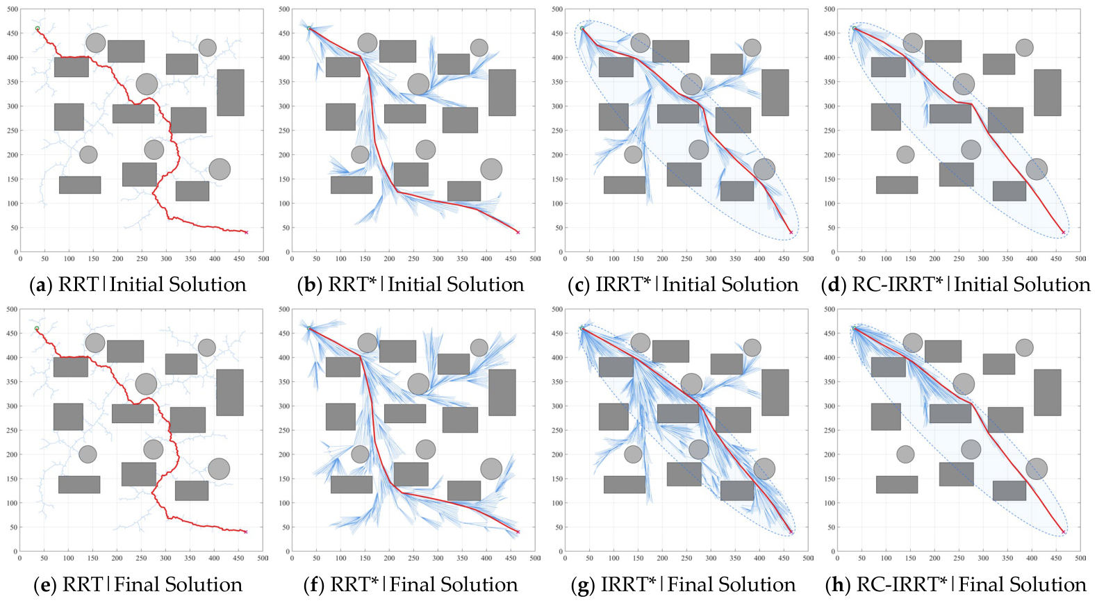
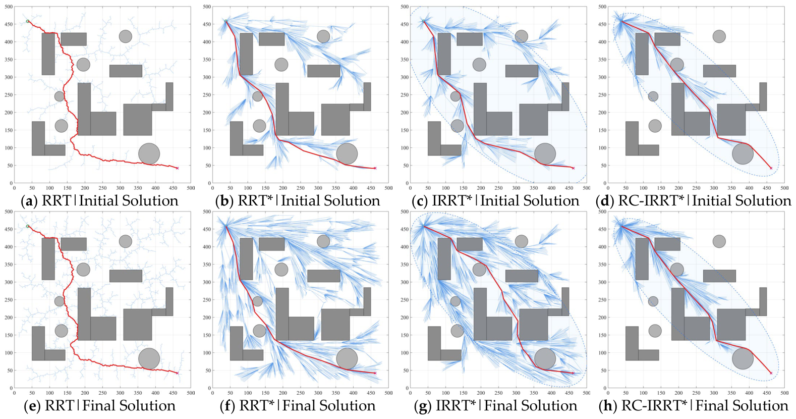
Figure 6 shows the initial and final planning results of the four algorithms in the sparse environment. RRT quickly finds a feasible path, but the resulting trajectory contains obvious detours and frequent turning points. RRT* and Informed-RRT* improve the path through rewiring and informed sampling, but their tree expansion remains relatively dispersed in the free space. By contrast, RC-Informed-RRT* generates a more compact search tree and a smoother final path that is closer to the effective feasible corridor.

For brevity, Informed-RRT* and RC-Informed-RRT* are abbreviated as IRRT* and RC-IRRT*, respectively, in the result figures.

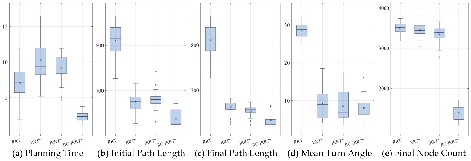
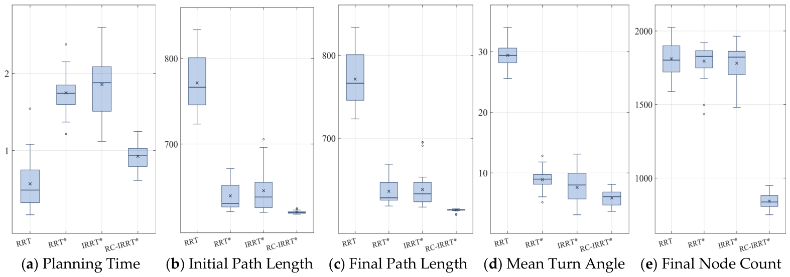
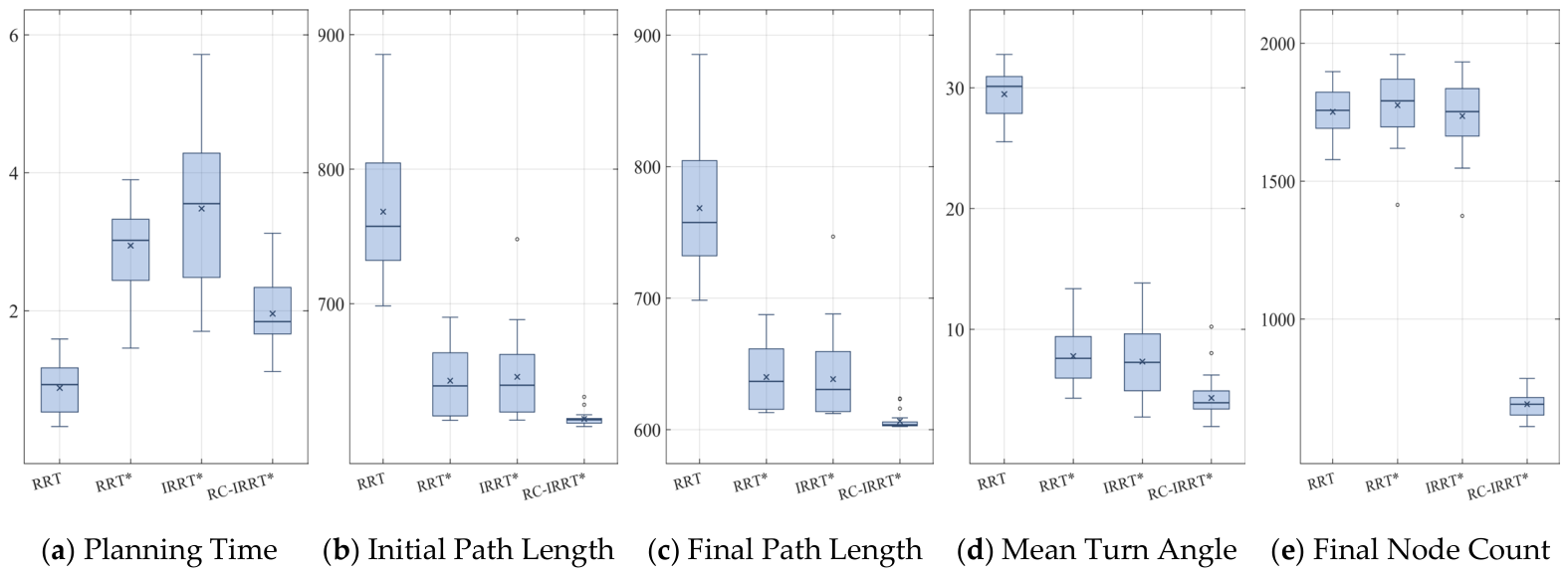
Figure 7 presents the corresponding box plots of the five continuous metrics. The distributions show that RC-Informed-RRT* not only achieves lower values in planning time, final path length, mean turn angle, and final node count than RRT* and Informed-RRT*, but also exhibits smaller variability in repeated trials. This indicates that the proposed method provides better stability in addition to improved overall performance.

The quantitative results are listed in

Table 3. Simulation results in the sparse environment.

Algorithm	Tp (s)	Li	Lf	$\overline{\mathit{\theta }}$ (deg)	Nf	Sr
RRT	0.58 ± 0.31	773.47 ± 36.75	773.47 ± 36.75	29.56 ± 2.13	1813.45 ± 108.14	96.00% (48/50)
RRT*	1.77 ± 0.22	641.13 ± 16.72	637.52 ± 14.62	8.82 ± 1.61	1797.72 ± 112.64	100.00% (50/50)
Informed-RRT*	1.88 ± 0.41	648.65 ± 24.17	640.47 ± 23.21	7.59 ± 3.07	1783.24 ± 124.36	100.00% (50/50)
RC-Informed-RRT*	0.93 ± 0.16	622.31 ± 1.96	615.32 ± 1.74	5.97 ± 1.37	844.41 ± 49.62	100.00% (50/50)

. Across the 50 perturbed trials, RRT succeeds in 48 cases (96.00%), whereas RRT*, Informed-RRT*, and RC-Informed-RRT* each succeed in all 50 trials. The small geometric perturbations therefore introduce limited additional variability without changing the overall feasibility of the sparse environment for the optimization-based planners.

RRT has the shortest mean planning time (0.58 ± 0.31 s), but its final path length remains 773.47 ± 36.75 and its mean turn angle is 29.56 ± 2.13°, indicating poor path quality despite fast exploration. RC-Informed-RRT* requires 0.93 ± 0.16 s on average, which is 47.46% lower than RRT* and 50.53% lower than Informed-RRT*. Its final path length is 615.32 ± 1.74, representing reductions of 3.48% and 3.93% relative to RRT* and Informed-RRT*, respectively.

RC-Informed-RRT* also gives the lowest mean turn angle (5.97 ± 1.37°) and the smallest final tree (844.41 ± 49.62 nodes). The final node count is reduced by 53.03% relative to RRT* and by 52.65% relative to Informed-RRT*. Together with its 100.00% success rate, these results show that the proposed mechanisms improve path geometry and substantially reduce redundant tree growth in the sparse environment.

4.5. Dense Environment

The dense environment contains more obstacles with a more compact spatial distribution. Compared with the sparse map, this environment produces more invalid extensions and requires the planner to search through several locally constrained free regions. Therefore, it is used to evaluate the ability of each algorithm to reduce redundant expansion and maintain reliable planning in cluttered spaces.

Figure 8 shows the initial and final planning results of the four algorithms in the dense environment. RRT generates a feasible path in most trials, but the path is highly tortuous and the success rate decreases because several random expansions are blocked by dense obstacles. RRT* and Informed-RRT* improve the path quality through rewiring and heuristic sampling, but their search trees still spread over a large area. In contrast, RC-Informed-RRT* concentrates more samples around safer and more useful regions, producing a shorter and smoother final path with fewer redundant branches.

Figure 9 presents the box plots of the five continuous metrics in the dense environment. The proposed RC-Informed-RRT* shows lower median values and narrower distributions in final path length, mean turn angle, and final node count. This indicates that the risk-density-aware corridor sampling and improvement-bound rejection reduce unstable tree growth in obstacle-dense regions.

The quantitative results are listed in

Table 4. Simulation results in the dense environment.

Algorithm	Tp (s)	Li	Lf	$\overline{\mathit{\theta }}$ (deg)	Nf	Sr
RRT	0.89 ± 0.34	769.47 ± 46.62	769.47 ± 46.62	30.14 ± 2.15	1768.48 ± 94.88	86.00% (43/50)
RRT*	2.97 ± 0.83	645.72 ± 24.86	643.56 ± 27.26	7.82 ± 2.72	1779.23 ± 123.48	92.00% (46/50)
Informed-RRT*	3.64 ± 1.26	646.57 ± 29.72	639.56 ± 31.22	7.57 ± 2.97	1738.52 ± 121.26	94.00% (47/50)
RC-Informed-RRT*	1.97 ± 0.47	617.24 ± 6.41	608.34 ± 6.57	4.56 ± 1.72	693.20 ± 46.87	100.00% (50/50)

. Under the 50 perturbed trials, RRT succeeds in 43 cases (86.00%), RRT* in 46 cases (92.00%), and Informed-RRT* in 47 cases (94.00%). RC-Informed-RRT* succeeds in all 50 trials, indicating higher reliability under dense obstacle distributions and small local geometric variations.

Although RRT has the lowest mean planning time (0.89 ± 0.34 s), its final path length remains 769.47 ± 46.62 and its mean turn angle reaches 30.14 ± 2.15°, showing poor path quality and smoothness. RC-Informed-RRT* reduces mean planning time to 1.97 ± 0.47 s, corresponding to reductions of 33.67% relative to RRT* and 45.88% relative to Informed-RRT*. This indicates that the proposed sampling regulation and pre-insertion rejection reduce unnecessary tree expansion and rewiring in cluttered regions.

RC-Informed-RRT* obtains a final path length of 608.34 ± 6.57, which is 5.47% shorter than RRT* and 4.88% shorter than Informed-RRT*. Its mean turn angle decreases to 4.56 ± 1.72°. The final node count is 693.20 ± 46.87, corresponding to reductions of 61.04% and 60.13% relative to RRT* and Informed-RRT*, respectively. The combination of lower redundancy, shorter paths, and a 100.00% success rate demonstrates the strongest overall advantage of RC-Informed-RRT* in the dense environment.

4.6. Narrow-Passage Environment

The narrow-passage environment contains several locally constrained regions and limited free-space connections between obstacles. Compared with the sparse and dense maps, the feasible route is more dependent on passing through narrow gaps, which makes excessive random expansion and premature search bias more likely to reduce planning efficiency. Therefore, this environment is used to evaluate whether each planner can maintain exploration capability while focusing tree growth on useful passage regions.

Figure 10 shows the initial and final planning results of the four algorithms in the narrow-passage environment. RRT can find feasible paths under the given iteration limit, but the resulting trajectory contains obvious detours and frequent turning changes. RRT* and Informed-RRT* improve path quality through rewiring and informed sampling, yet their search trees still contain many branches distributed around constrained regions. By contrast, RC-Informed-RRT* generates a more compact tree and guides the search toward the effective passage region while preserving sufficient exploration to pass through narrow areas.

Figure 11 presents the box plots of the five continuous metrics in the narrow-passage environment. The distributions show that RC-Informed-RRT* achieves clearly lower planning time and final node count than the baseline algorithms. Its final path length is also smaller than those of RRT*, Informed-RRT*, and RRT, while the mean turn angle remains close to that of Informed-RRT* and much lower than that of RRT. This indicates that the proposed corridor regulation and improvement-bound rejection mechanisms reduce redundant tree growth without losing the ability to search through constrained passages.

The quantitative results are listed in

Table 5. Simulation results in the narrow-passage environment.

Algorithm	Tp (s)	Li	Lf	$\overline{\mathit{\theta }}$ (deg)	Nf	Sr
RRT	7.08 ± 2.34	810.35 ± 37.42	810.35 ± 37.42	27.24 ± 1.72	3501.38 ± 148.71	98.00% (49/50)
RRT*	10.78 ± 2.91	678.14 ± 22.52	660.68 ± 13.71	9.10 ± 3.56	3449.14 ± 170.66	98.00% (49/50)
Informed-RRT*	9.19 ± 1.92	681.36 ± 19.38	653.84 ± 13.67	8.53 ± 4.20	3344.47 ± 217.31	100.00% (50/50)
RC-Informed-RRT*	2.32 ± 0.72	639.37 ± 18.31	632.70 ± 16.58	8.06 ± 2.67	1396.98 ± 194.52	100.00% (50/50)

. RRT and RRT* each succeed in 49 of 50 trials (98.00%), while Informed-RRT* and RC-Informed-RRT* both achieve a 100.00% success rate. Thus, the narrow-passage map remains highly feasible under the selected iteration budget, but the perturbed trials reveal small reliability differences that were not visible in a single fixed geometry.

RC-Informed-RRT* reduces the mean planning time from 10.78 ± 2.91 s for RRT* to 2.32 ± 0.72 s, a reduction of 78.48%. Relative to Informed-RRT*, the reduction is 74.76%. RRT is computationally cheaper than RRT* and Informed-RRT*, but its final path length remains 810.35 ± 37.42 and its mean turn angle is 27.24 ± 1.72°, confirming the trade-off between fast unguided exploration and path quality.

RC-Informed-RRT* obtains a final path length of 632.70 ± 16.58, which is 4.24% shorter than RRT* and 3.23% shorter than Informed-RRT*. Its mean turn angle is 8.06 ± 2.67°, slightly lower than those of RRT* and Informed-RRT*. More importantly, the final node count decreases to 1396.98 ± 194.52, representing reductions of 59.50% and 58.23% relative to RRT* and Informed-RRT*, respectively. These results show that the soft corridor retains the exploration needed for constrained passages while substantially reducing redundant expansion.

4.7. W-Shaped Environment

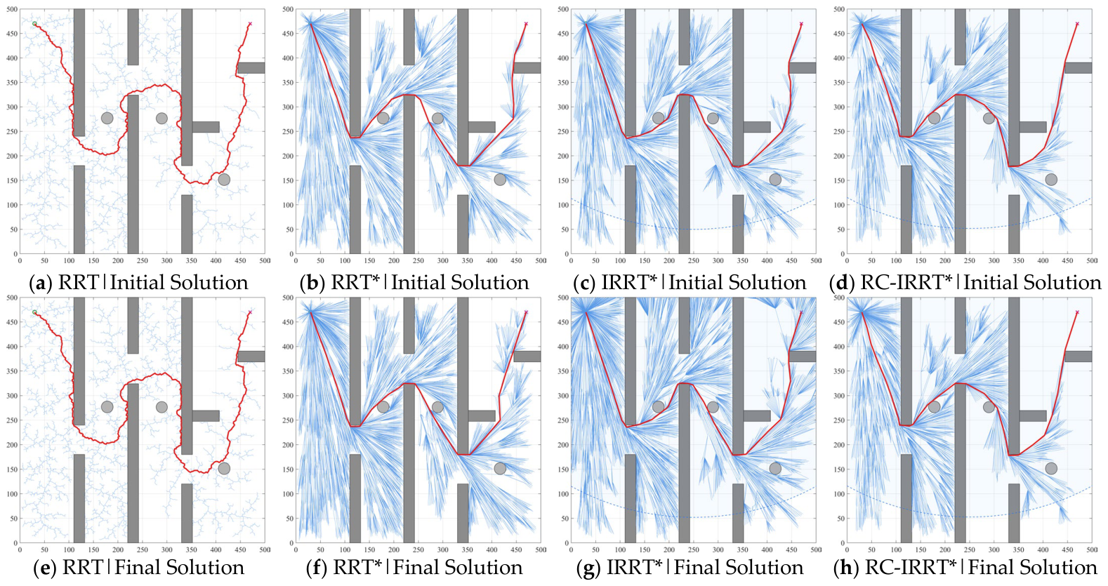
The W-shaped environment is a detour-dominated map with several long obstacle barriers. In this case, the feasible route deviates significantly from the direct start-to-goal direction and requires multiple turning detours. Since RC-Informed-RRT* uses a reference-corridor-guided sampling mechanism, its advantage may be weakened when the effective route is not naturally aligned with the initial geometric reference. Therefore, this map is used as a non-preferred test case to evaluate whether the proposed method can still preserve feasibility and efficiency under unfavorable corridor-guidance conditions.

Figure 12 shows the initial and final planning results of the four algorithms in the W-shaped environment. RRT produces highly tortuous paths and some trials fail to reach the goal within the iteration limit. RRT* and Informed-RRT* can improve the path through optimization, but their search trees still contain many redundant branches. Although RC-Informed-RRT* does not show an obvious advantage over RRT* or Informed-RRT* during the early detour exploration, its advantage becomes more evident in the middle and later portions of the route, especially in the relatively open region near the goal, where redundant branches are further suppressed while the required detour path is still maintained.

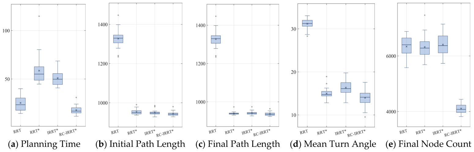
Figure 13 presents the box plots of the five continuous metrics. In this map, the path-length difference among RRT*, Informed-RRT*, and RC-Informed-RRT* is relatively small, because the feasible route is strongly constrained by the obstacle layout. However, RC-Informed-RRT* shows clear advantages in planning time and final node count, indicating that the proposed mechanisms still reduce redundant exploration in a detour-dominated environment.

The quantitative results are listed in

Table 6. Simulation results in the W-shaped environment.

Algorithm	Tp (s)	Li	Lf	$\overline{\mathit{\theta }}$ (deg)	Nf	Sr
RRT	26.14 ± 7.47	1334.65 ± 45.07	1334.65 ± 45.07	31.48 ± 1.24	6342.56 ± 354.27	90.00% (45/50)
RRT*	57.46 ± 15.47	954.34 ± 13.48	938.71 ± 4.11	14.78 ± 1.26	6323.47 ± 377.48	96.00% (48/50)
Informed-RRT*	51.13 ± 7.64	950.84 ± 11.78	943.47 ± 9.36	16.41 ± 1.39	6410.98 ± 396.37	98.00% (49/50)
RC-Informed-RRT*	18.81 ± 4.08	943.78 ± 10.28	936.36 ± 9.89	13.76 ± 2.17	4108.37 ± 167.43	98.00% (49/50)

. RRT succeeds in 45 of 50 trials (90.00%), RRT* in 48 trials (96.00%), and both Informed-RRT* and RC-Informed-RRT* in 49 trials (98.00%). Thus, RC-Informed-RRT* matches the reliability of Informed-RRT* in the W-shaped environment while retaining a clear efficiency advantage under the perturbed detour-dominated instances.

In this unfavorable map, RC-Informed-RRT* still achieves the shortest mean planning time among the optimization-based planners. Its value of 18.81 ± 4.08 s is 67.26% lower than RRT* and 63.21% lower than Informed-RRT*. The probabilistic pre-solution corridor treatment and fallback sampling retain detour discovery before a feasible path is established, while improvement-bound rejection suppresses low-contribution insertions and rewiring after a solution becomes available.

Because the W-shaped obstacle layout strongly constrains the feasible route, the final-path-length differences among the three RRT*-based planners are small. RC-Informed-RRT* nevertheless obtains the shortest final path (936.36 ± 9.89), which is 0.25% shorter than RRT* and 0.75% shorter than Informed-RRT*, and it also gives the smallest mean turn angle (13.76 ± 2.17°). Its final node count is reduced to 4108.37 ± 167.43, 35.03% below RRT* and 35.92% below Informed-RRT*. These results indicate that the method preserves reliability while reducing redundant tree growth even when the initial corridor direction is unfavorable.

4.8. Additional Validation Experiments

To further validate the contribution of the proposed mechanisms and the fairness of the parameter settings used in the comparative experiments, additional validation experiments were conducted, including a sequential ablation study and a goal-bias sensitivity analysis.

4.8.1. Sequential Ablation Study

To isolate the incremental contribution of the three proposed mechanisms under a controlled setting, a sequential cumulative ablation study was conducted in the dense environment using the same maximum iteration budget, step size, collision-checking conditions, small geometric perturbation protocol, and 50-trial evaluation used in the main comparison. The four variants were Informed-RRT* (baseline), Informed-RRT*+A, Informed-RRT*+A+B, and Informed-RRT*+A+B+C, where A denotes risk-density-aware corridor sampling, B denotes improvement-bound rejection, and C denotes search-state-regulated goal bias. The +A+B+C configuration corresponds to the complete RC-Informed-RRT*.

In addition to the five continuous metrics used in the four-environment comparison, three search-process indicators were logged: time to the first feasible solution, first-solution iteration, and the iteration at which the final best solution was first reached. These indicators provide a compact convergence-oriented description of both solution onset and subsequent optimization progress. Following the metric-specific aggregation rule in Section 4.3, planning time and final node count are reported as mean ± standard deviation over all 50 trials, including unsuccessful runs. First-solution time, initial and final path lengths, first-solution iteration, best-solution iteration, and mean turn angle are reported over successful runs only because these quantities require a feasible solution. Success rate is computed over all 50 trials.

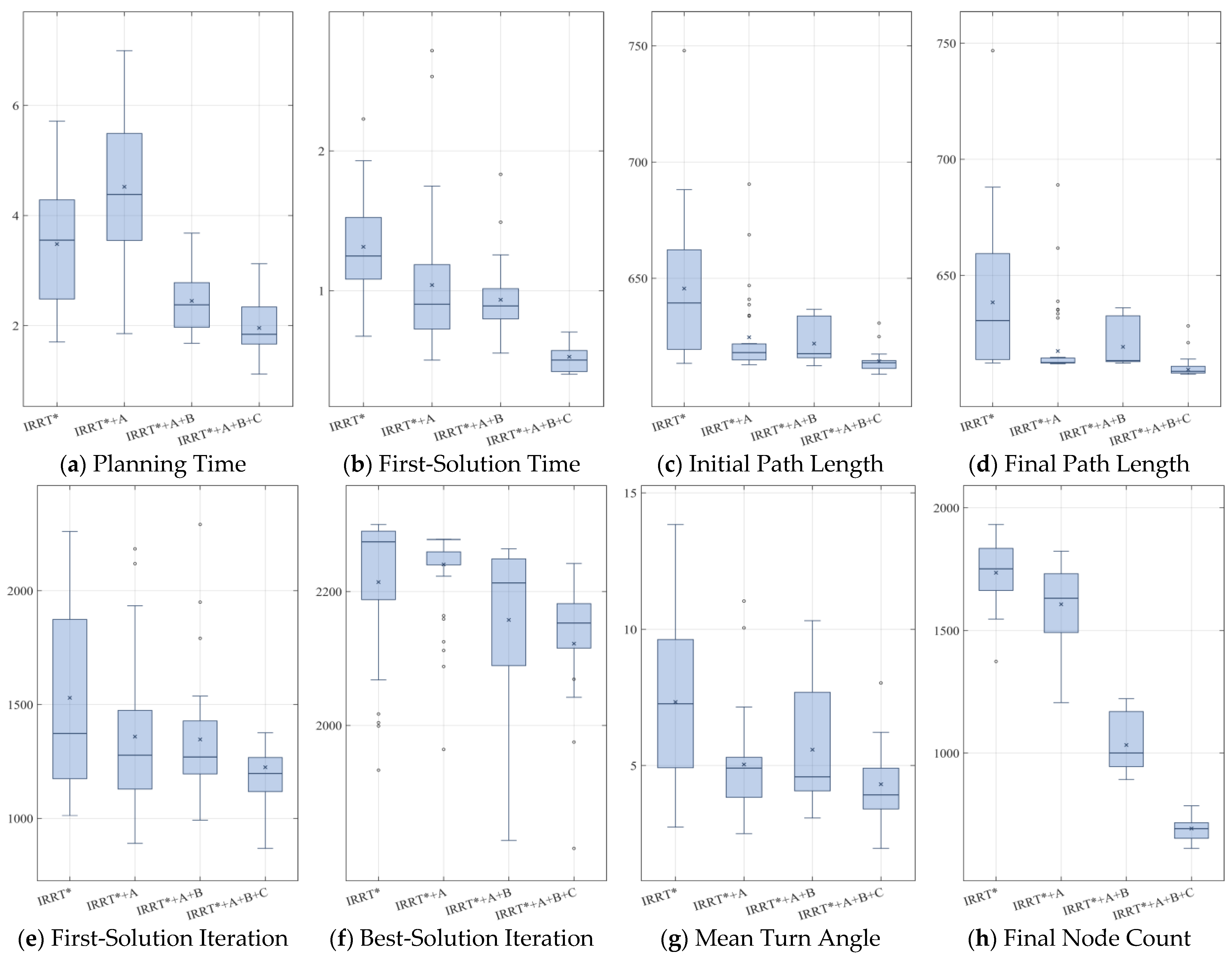
Figure 14 shows the distributions of the eight recorded performance indicators. The box plots provide a visual comparison of both central tendency and trial-to-trial variability as the three mechanisms are introduced sequentially.

The corresponding quantitative results are summarized in

Table 7. Sequential ablation results in the dense environment.

Algorithm	Tp (s)	Tfirst (s)	Li	Lf	Ifirst	Ibest	$\overline{\mathit{\theta }}$ (deg)	Nf	Sr
IRRT*	3.47 ± 1.18	1.31 ± 0.36	645.56 ± 29.80	638.44 ± 29.05	1529.52 ± 394.37	2214.28 ± 111.88	7.31 ± 2.96	1735.77 ± 124.87	94.00% (47/50)
IRRT*+A	4.52 ± 1.33	1.04 ± 0.53	624.63 ± 17.62	617.41 ± 17.55	1358.93 ± 346.14	2240.57 ± 108.01	5.04 ± 2.47	1607.37 ± 154.66	98.00% (49/50)
IRRT*+A+B	2.45 ± 0.52	0.93 ± 0.26	621.91 ± 8.82	619.22 ± 9.67	1346.87 ± 317.36	2157.60 ± 139.25	5.58 ± 2.18	1033.00 ± 109.98	98.00% (49/50)
IRRT*+A+B+C	1.95 ± 0.44	0.53 ± 0.13	614.38 ± 5.86	608.74 ± 6.57	1224.50 ± 320.51	2122.17 ± 114.13	4.29 ± 1.68	690.97 ± 44.09	100.00% (50/50)

. The values in the table are consistent with the box-plot statistics and allow the incremental changes introduced at each stage to be compared directly.

Adding mechanism A improves early search and path-related indicators but introduces additional risk-density and corridor-evaluation overhead. Relative to the Informed-RRT* baseline, +A reduces first-solution time from 1.31 ± 0.36 s to 1.04 ± 0.53 s, initial path length from 645.56 ± 29.80 to 624.63 ± 17.62, final path length from 638.44 ± 29.05 to 617.41 ± 17.55, and mean turn angle from 7.31 ± 2.96° to 5.04 ± 2.47°. First-solution iteration also decreases from 1529.52 ± 394.37 to 1358.93 ± 346.14, and the success rate increases from 94.00% (47/50) to 98.00% (49/50). The total planning time, however, rises from 3.47 ± 1.18 s to 4.52 ± 1.33 s, showing the computational cost of corridor and risk evaluation before the rejection mechanism is added.

When mechanism B is added, the most pronounced changes occur in computational efficiency and tree compactness. Relative to +A, +A+B reduces planning time from 4.52 ± 1.33 s to 2.45 ± 0.52 s and final node count from 1607.37 ± 154.66 to 1033.00 ± 109.98, corresponding to reductions of 45.80% and 35.73%. Best-solution iteration also decreases from 2240.57 ± 108.01 to 2157.60 ± 139.25. Final path length changes slightly from 617.41 ± 17.55 to 619.22 ± 9.67 and mean turn angle from 5.04 ± 2.47° to 5.58 ± 2.18°, while the success rate remains 98.00% (49/50). This small path-quality trade-off is consistent with the finite-horizon role of the improvement-bound filter: it suppresses low-contribution insertions and rewiring rather than preserving every marginal improvement.

Adding mechanism C further improves first-solution efficiency and search compactness. Relative to +A+B, first-solution time decreases from 0.93 ± 0.26 s to 0.53 ± 0.13 s, a reduction of 43.01%, and first-solution iteration decreases from 1346.87 ± 317.36 to 1224.50 ± 320.51. Planning time is further reduced to 1.95 ± 0.44 s and final node count to 690.97 ± 44.09. At the same time, final path length decreases to 608.74 ± 6.57 and mean turn angle to 4.29 ± 1.68°. The complete +A+B+C variant therefore combines faster goal connection, lower tree redundancy, and a 100.00% success rate (50/50).

Overall, relative to the Informed-RRT* baseline, the complete +A+B+C configuration reduces planning time by 43.80%, first-solution time by 59.54%, initial path length by 4.83%, final path length by 4.65%, mean turn angle by 41.31%, and final node count by 60.19%. The success rate increases from 94.00% (47/50) to 100.00% (50/50). The cumulative results support different stage-wise roles for the three mechanisms: A primarily improves search guidance and path geometry, B mainly reduces computation and tree redundancy, and C accelerates goal connection and further compacts the search. Because the variants are cumulative, these effects should be interpreted as incremental contributions in the tested integration order rather than independent main effects free of interaction.

4.8.2. Goal-Bias Sensitivity and Baseline Fairness

To examine the sensitivity and fairness of the fixed baseline goal-bias probability, a one-factor experiment was conducted with Informed-RRT* in the dense environment. The fixed probability p_g was varied from 0.05 to 0.10 in increments of 0.01, and each setting was evaluated in 50 independent trials using the same iteration limit and small geometric perturbation protocol as the main dense-map experiment. The dense environment was selected because its cluttered geometry makes the trade-off between direct goal sampling and exploratory sampling particularly visible, while Informed-RRT* was selected because it is the closest structural baseline to RC-Informed-RRT*. The purpose of this experiment is not to identify a separate optimum for every algorithm-environment pair, but to select one balanced common fixed setting under a deliberately challenging condition and then hold that setting unchanged across the fixed-bias baseline planners and environments. The same metric-specific aggregation rule as in Section 4.3 was applied: planning time and final node count include all 50 trials, whereas first-solution time, initial and final path lengths, first-solution iteration, best-solution iteration, and mean turn angle are calculated from successful runs only.

As shown in

Table 8. Sensitivity of Informed-RRT* to the fixed goal-bias probability in the dense environment.

pg	Tp (s)	Tfirst (s)	Li	Lf	Ifirst	Ibest	$\overline{\mathit{\theta }}$ (deg)	Nf
0.05	3.26 ± 0.59	1.02 ± 0.18	646.37 ± 24.26	639.83 ± 23.83	1477.47 ± 245.94	2252.63 ± 43.08	6.88 ± 2.43	1735.89 ± 160.02
0.06	3.15 ± 0.51	1.06 ± 0.22	637.94 ± 31.16	633.35 ± 28.02	1411.95 ± 274.83	2231.60 ± 59.44	6.18 ± 3.02	1746.65 ± 88.89
0.07	3.11 ± 0.73	0.87 ± 0.29	633.58 ± 26.07	628.08 ± 25.97	1309.65 ± 369.96	2207.30 ± 119.71	5.44 ± 3.16	1768.40 ± 120.62
0.08	3.03 ± 0.77	0.86 ± 0.23	633.31 ± 26.70	633.09 ± 27.68	1285.58 ± 328.67	2208.21 ± 63.64	5.70 ± 2.93	1735.47 ± 123.72
0.09	3.21 ± 1.06	0.91 ± 0.38	635.85 ± 23.95	629.77 ± 26.35	1316.40 ± 475.68	2231.70 ± 56.28	5.58 ± 2.61	1735.15 ± 141.96
0.10	3.36 ± 0.89	0.80 ± 0.24	641.33 ± 32.25	634.82 ± 32.44	1277.10 ± 346.81	2254.05 ± 148.54	5.42 ± 2.75	1742.50 ± 100.18

Note: Values are reported as mean ± standard deviation. Planning time and final node count are calculated over all 50 trials, including failed runs. First-solution time, initial and final path lengths, first-solution iteration, best-solution iteration, and mean turn angle are calculated from successful runs because these quantities require a feasible solution. Each fixed goal-bias setting was evaluated in 50 independent trials. T_first denotes first-solution time; I_first denotes first-solution iteration; and I_best denotes the iteration at which the final best solution was first reached.

, the fixed goal-bias probability affects different aspects of the search in different ways, and no monotonic improvement is observed as p_g increases. Among the tested settings, p_g = 0.08 provides the most balanced overall behavior. It achieves the lowest mean planning time (3.03 ± 0.77 s) and the shortest mean initial path length (633.31 ± 26.70), while its first-solution iteration (1285.58 ± 328.67), best-solution iteration (2208.21 ± 63.64), and final node count (1735.47 ± 123.72) remain close to the best values observed across the six settings. Although individual metrics attain slightly lower values at adjacent settings—for example, the final path length at p_g = 0.07 and the first-solution time and mean turn angle at p_g = 0.10—these improvements are accompanied by degradation in other metrics, indicating a trade-off between stronger goal-directed expansion and exploration diversity.

Considering the eight recorded indicators jointly, p_g = 0.08 was selected as a balanced common setting for the fixed-bias baseline planners. Relative to p_g = 0.06, this setting reduces mean planning time by 3.81%, first-solution time by 18.87%, first-solution iteration by 8.95%, and mean turn angle by 7.77%, while the other indicators stay close to the best values among the tested settings. This choice is not claimed to be a universal optimum for every algorithm-environment pair. Rather, the same p_g = 0.08 is deliberately retained for RRT, RRT*, and Informed-RRT* in all four environments because p_g has the same operational role in each fixed-bias baseline: it controls the probability of direct goal sampling instead of invoking that planner’s non-goal sampling rule. Freezing one common value avoids algorithm-specific or map-specific retuning and provides a uniform control condition for comparison with the adaptive goal-bias strategy of RC-Informed-RRT*.

This sensitivity analysis concerns only the fixed goal-bias probability of the baseline planners. The adaptive goal-bias range [0.03, 0.28] of RC-Informed-RRT* is retained because it serves a different purpose: it bounds the state-dependent probability p_goal(i) rather than specifying a single fixed sampling probability.

4.9. Experimental Summary

The 50-trial results with small geometric perturbations show that RC-Informed-RRT* retains its main performance advantages across different obstacle distributions, while the magnitude of the improvement depends on the structure of the environment.

(i)

In the sparse environment, RC-Informed-RRT* maintains a 100.00% success rate, reduces final node count by more than 52% relative to both RRT* and Informed-RRT*, and produces shorter and smoother paths with low trial-to-trial variability.

(ii)

In the dense environment, RC-Informed-RRT* achieves a 100.00% success rate compared with 86.00–94.00% for the three baselines. Its risk-aware corridor and rejection mechanisms provide the clearest reductions in redundant tree growth and planning time under cluttered obstacle distributions.

(iii)

In the narrow-passage environment, RC-Informed-RRT* retains a 100.00% success rate while reducing planning time by 74.76% relative to Informed-RRT*. The soft corridor remains sufficiently permissive for passage exploration and reduces final node count by 58.23% relative to Informed-RRT*.

(iv)

In the W-shaped environment, where the nominal direct corridor is poorly aligned with the required detour, RC-Informed-RRT* reaches a 98.00% success rate, matching Informed-RRT*, while reducing planning time by 63.21% and final node count by 35.92% relative to Informed-RRT*. This result supports the role of probabilistic corridor regulation and fallback sampling in preserving detour exploration.

The additional validation supports the internal interpretation of these results. Sequential ablation shows that corridor sampling mainly improves guidance and path geometry, improvement-bound rejection mainly reduces computational cost and tree redundancy, and search-state-regulated goal bias further accelerates first-solution generation. The goal-bias sensitivity experiment identifies p_g = 0.08 as a balanced fixed setting for the baseline planners. The small coordinate perturbations increase local geometric diversity, but they do not replace validation on real maps, dynamic obstacles, or kinodynamic systems; these remain outside the scope of the present study.

5. Conclusions

This paper proposes RC-Informed-RRT*, a risk-density-aware corridor-constrained extension of Informed-RRT*. The method coordinates three mechanisms: a soft corridor sampler that combines corridor deviation, obstacle clearance, and local density; an improvement-bound rejection rule that filters low-contribution nodes after provisional parent selection; and a search-state-regulated goal bias that adapts target-oriented sampling to goal proximity, stagnation, and planning phase. The integrated design aims to improve guidance and tree compactness without converting the corridor into a rigid constraint.

Comparative simulations were conducted in sparse, dense, narrow-passage, and W-shaped environments using 50 randomized trials per algorithm and small perturbations of the nominal start/goal and obstacle locations. Relative to Informed-RRT*, RC-Informed-RRT* reduces mean planning time by 45.88–74.76% and final node count by 35.92–60.13% across the four environments, while the final path length is reduced by 0.75–4.88%. The proposed method achieves a 98–100% success rate across the four maps. Sequential ablation further distinguishes the incremental roles of the three mechanisms, and the goal-bias sensitivity study supports the use of p_g = 0.08 for the fixed baseline planners.

The current validation remains limited to two-dimensional static maps with small local geometric perturbations. Although this protocol reduces dependence on a single fixed start-goal pair and exact obstacle placement, it does not represent large-scale random maps, real sensor-derived environments, dynamic obstacles, or robot kinematic and kinodynamic constraints. Future work will extend the method to three-dimensional and dynamic settings, evaluate it on real or sensor-derived maps and physical platforms, and investigate adaptive parameter regulation and trajectory-level smoothing under motion constraints.