On Sampled Sequence Representations at Discontinuities and Their Impact on Discrete Convolution

Abstract

If one compares the continuous-time convolution outputs with their sampled discrete counterparts, one may observe slight differences even when the sampling process itself is otherwise straightforward. This issue becomes noticeable when one or both continuous-time signals have a discontinuity at the sampling instant, such as t = 0. In this paper, we revisit this issue and explain its root causes: the treatment of midpoint values at discontinuities and the sampling-period scaling that appears when a continuous-time convolution is approximated in discrete time. Although the midpoint rule is not new, we show how this classical result can be used systematically to construct sampled sequence representations that are consistent with inverse-transform reconstruction at discontinuities. Based on this viewpoint, we derive midpoint-consistent sampled sequence representations for quite a few representative functions, and we show the corresponding implications for sampled convolution formulae. Several examples are used to compare conventional discrete formulae with midpoint-consistent sampled formulae and with samples of the continuous-time results. The proposed formulation is intended for sampled continuous-time signals at discontinuities; it is not meant to replace standard native discrete-time conventions used in digital signal processing.

1. Introduction

Since the invention of fast Fourier transform (FFT) in the 1960s [1] and the discrete cosine transform (DCT) in the 1970s [2], digital and image processing algorithms have been widely used in many applications, including acoustic processing [3], voice recognition [4], face recognition [5], remote sensing [6], and many others. In the processing pipeline, continuous signals are discretized to discrete sequences. We normally expect the discrete signals to be the sampled versions of the corresponding continuous signals. This is mostly true when the sampling rate is high. However, in some cases such as the convolution of two step functions, there is a small difference between the discrete time and the continuous time versions. In particular, the convolution of unit step functions $u\left(t\right)$ and $u\left(t\right)$ is given by $tu\left(t\right)$ in the continuous domain from Table 2 in [7]; the convolution of $u\left[n\right]$ and $u\left[n\right]$ in the discrete domain is given by $(n+1)u\left[n\right]$ according to Table 3 in [7]. If one samples $tu\left(t\right)$, one will obtain a sequence of $nTu\left[n\right]$, not $(n+1)u\left[n\right]$. Why is the sampled version of $tu\left(t\right)$ different from the discrete convolution of two discrete time step functions of $u\left[n\right]$? Moreover, the discrete convolution formulae in Table 3 [7] do not have any connection with the sampling interval T. The consequence is that the continuous convolution outputs and the discrete convolution outputs are not the same.

Another example is the convolution between the unit step $u\left(t\right)$ and the ramp function $tu\left(t\right)$, which is given by $0.5t^{2}u\left(t\right)$ from Table 2 of [7]. However, if one carries out the discrete time convolution between the corresponding discretized functions $u\left[n\right]$ and $nu\left[n\right]$, one obtains $0.5n(n+1)u\left[n\right]$ from Table 3 of [7]. The sampled version of $0.5t^{2}u\left(t\right)$ is, however, $0.5n^2{T}^{2}u\left[n\right]$, which is different from $0.5n(n+1)u\left[n\right]$. Multiplying $T^2$ to $0.5n(n+1)u\left[n\right]$ will close the gap between the sampled version, $0.5n^2{T}^{2}u\left[n\right]$, and the scaled discrete version, $0.5n(n+1)T^{2}u\left[n\right]$. But why do we need to multiply by $T^2$? What is going on here? Engineers may be confused by the above observations. Actually, there are many instances where the discrete-time convolution results are different from the sampled versions of the continuous convolution.

In this paper, we use examples with equations, figures, and metrics to illustrate the above issues between continuous-time convolutions and their sampled discrete counterparts. We then identify the root causes of the observed differences. One root cause is the discontinuity at t = 0 for functions such as the unit step u(t). A second root cause is the sampling-period scaling that arises when continuous-time convolution is approximated in discrete time. Classical results from Fourier analysis and distribution theory show that, at a point of jump discontinuity, the inverse transform reconstruction converges to the average of the left- and right-hand limits. The present paper does not claim this midpoint result as new. Rather, the goal is to apply it systematically to sampled sequence representations and to show its consequences for convolution formulae when the underlying signal is a sampled continuous-time signal with a discontinuity at the sampling instant.

It is important to distinguish between two different objects. A native discrete-time sequence is defined directly on the integer index n and may legitimately adopt the standard engineering convention u [0] = 1. A sampled continuous-time sequence, by contrast, is obtained from a continuous-time signal x(t) evaluated at t = nT. When x(t) has a jump discontinuity at the sampling instant, a midpoint-consistent sampled representation uses the average of the one-sided limits at that point. The results in this paper concern the latter setting. Therefore, our conclusions should be interpreted as a consistency analysis for sampled continuous-time representations at discontinuities, not as a universal replacement for standard native discrete-time DSP conventions.

For notational clarity, Section 3 will denote native discrete-time sequences by $x_d\left[n\right]$ and sampled sequences by $x_s\left[n\right]$.

Classical Fourier analysis and distribution-theoretic results establish the midpoint value at jump discontinuities under inverse-transform reconstruction. Standard DSP textbooks [7,8,9,10,11], however, often adopt native discrete-time conventions for practical modeling. Sampled-data and digital-control texts [12,13,14], on the other hand, emphasize the relationship between continuous-time systems, sampling, and discrete-time approximations. The present paper focuses on the interface between these two viewpoints: it examines how the classical midpoint rule should be represented when a discrete sequence is interpreted specifically as a sampled version of an underlying continuous-time signal, and how that choice affects sampled-data convolution formulae.

Our contributions are as follows. First, we clarify the distinct roles of midpoint sampling at discontinuities and sampling-period scaling in explaining why sampled continuous-time convolution results can differ from conventional discrete formulae. Second, we present midpoint-consistent sampled representations for several representative functions and a general class of transfer functions. Third, we derive the corresponding implications for sampled convolution formulae. Finally, we use several examples, including a filter example, to compare conventional discrete results, midpoint-consistent sampled results, and sampled continuous-time results.

This paper is organized as follows. In Section 2, we will use an example to illustrate some issues in the convolution of two discrete unit step functions. In Section 3, we will provide the background for the inverse Fourier transform and Laplace transform. We will illustrate that the initial value $x\left(0\right)$ of the inverse Fourier transform of $X\left(\omega \right)$ is one-half of the magnitude of the discontinuity. Similarly, we will illustrate that the initial value $x\left(0\right)$ of the inverse Laplace transform of $X\left(s\right)$ is also one-half of the magnitude of the discontinuity. We will also review the proper relationship between continuous convolution and discrete convolution. We then present the root cause of the issues raised in Section 2. In Section 4, we will then derive and present the formulae for discrete sample sequences of continuous functions with and without discontinuities and the formulae for discrete convolutions. In Section 5, we present four examples to illustrate the differences between various convolution outputs, including continuous convolution, conventional discrete convolution, and the midpoint-consistent sampled convolution. Finally, we conclude the paper with a few remarks in Section 6. In the Appendix A, Appendix B, Appendix C, Appendix D and Appendix E, we present detailed derivations for those formulae mentioned in Section 4.

2. Issues

Let us use the convolution of two step functions to illustrate the issues. The continuous step function is defined as

$$u\left(t\right)=\left\{\begin{array}{cc}1,\hfill & t\ge 0\hfill \\ 0,\hfill & t<0\hfill \end{array}\right.$$

(1)

The conventional discrete-time step sequence, denoted later by $u_d[n]$, is defined as [7]

$$u[n]=\left\{\begin{array}{cc}1,\hfill & n\ge 0\hfill \\ 0,\hfill & n<0\hfill \end{array}\right.$$

(2)

When one performs the continuous convolution of two step functions, one obtains (Table 2 of [7])

$$y\left(t\right)=tu\left(t\right)=\left\{\begin{array}{cc}t,\hfill & t\ge 0\hfill \\ 0,\hfill & t<0\hfill \end{array}\right.$$

(3)

When one performs the discrete convolution of two step functions, one gets (Table 3 of [7])

$$y[n]=\left(n+1\right)u\left(n\right)=\left\{\begin{array}{cc}n+1,\hfill & n\ge 0\hfill \\ 0,\hfill & n<0\hfill \end{array}\right.$$

(4)

If we compare (3) and (4), one immediately notices that the sampling interval T is not explicitly present in (4). One should always keep in mind that at each discrete index n, the time at the nth sample is nT. We will see in Section 3 that, in order to ensure the discrete convolution outputs to have a similar magnitude as the continuous convolution outputs, we need to multiply one of the input sequences by T. Hence, the discrete convolution output in (4) should be replaced by

$$y\left[n\right]=\left(n+1\right)Tu\left(n\right)$$

(5)

We call the discrete convolution output in (5) the scaled discrete convolution output.

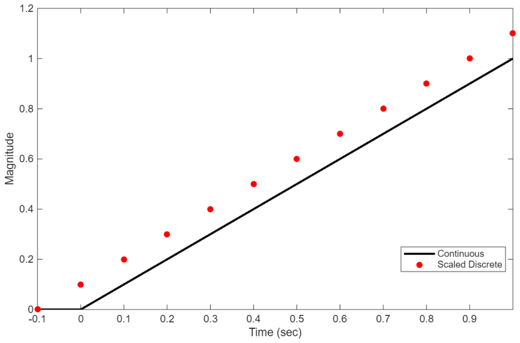
Now let us use a table and a figure to illustrate another issue between continuous and discrete convolutions.

Table 1. Comparison of continuous and discrete convolution outputs of two step functions. T = 0.1.

Time (s)	0	0.1	0.2	0.3
Sampling index n	0	1	2	3
Continuous convolution (3): tu(t)	0	0.1	0.2	0.3
Discrete convolution (4): $(n+1)u\left[n\right]$	1	2	3	4
Scaled discrete convolution (5): $(n+1)Tu\left[n\right]$	0.1	0.2	0.3	0.4

tabulates the continuous and discrete convolution results for several time instants. Here, we assume that the sampling interval T is 0.1 s. First, we observe from Table 1 that the discrete convolution outputs in row 4 are an order of magnitude larger than the continuous values. Second, even if we take the sampling interval T into account by multiplying the discrete convolution outputs in row 4 by T, the continuous (row 3) and scaled discrete convolution outputs (row 5) are still different. Figure 1 shows the difference between the continuous and the scaled discrete convolution results. Of course, one can argue that the difference is so small and can be ignored if T is small. However, in some applications, the sampling interval may not be small and this error may have some undesirable consequences.

3. Background and Explanations of the Issues in Section 2

Before presenting the transform-based arguments, we distinguish three related objects. Let $x_c\left(t\right)$ denote a continuous-time signal. Let $x_d\left[n\right]$ denote a native discrete-time sequence defined directly on the integer index n. Let $x_s\left[n\right]$ denote a sampled sequence obtained from $x_c\left(t\right)$ with sampling period T. If $x_c\left(t\right)$ is continuous at t = nT, then $x_s\left[n\right]=x_c\left(nT\right)$. If $x_c\left(t\right)$ has a jump discontinuity at t = 0, then under the midpoint-consistent sampled convention used in this paper, we set $x_s\left[0\right]$ = [x(0⁻) + x(0⁺)]/2. Throughout the paper, we use δ(t) to denote the continuous-time Dirac delta and δ[n] to denote the discrete-time Kronecker impulse.

Let us consider a signal with discontinuity at t = 0,

$$x\left(t\right)=e^{-pt}u\left(t\right)$$

(6)

where p > 0 and $u\left(t\right)$ is the unit step function. Note that for $x\left(t\right),$ there is a jump of 0 to 1 from $t=0^{-}$ to $t=0^{+}$. The corresponding Fourier transform $X\left(\omega \right)$ and Laplace transform $X\left(s\right)$ are respectively given by

$$\begin{array}{cc}\hfill X\left(\omega \right)& ={\int }_{-\infty }^{\infty }x\left(t\right)e^{-j\omega t}dt\hfill \\ & ={\int }_0^{\infty }{e}^{-pt}{e}^{-j\omega t}dt\hfill \\ & ={\displaystyle \frac{1}{p+j\omega }}\hfill \end{array}$$

(7)

$$\begin{array}{cc}\hfill X\left(s\right)& ={\int }_{-\infty }^{\infty }x\left(t\right)e^{-st}dt\hfill \\ & ={\int }_0^{\infty }{e}^{-pt}{e}^{-st}dt\hfill \\ & ={\displaystyle \frac{1}{p+s}}\hfill \end{array}$$

(8)

3.1. Inverse Fourier Transform of $X\left(\omega \right)$ at t = 0

The inverse Fourier transform of (7) is given by

$$\begin{array}{cc}\hfill x\left(t\right)& ={\displaystyle \frac{1}{2\pi }}{\int }_{-\infty }^{\infty }X\left(\omega \right)e^{j\omega t}d\omega \hfill \\ & ={\displaystyle \frac{1}{2\pi }}{\int }_{-\infty }^{\infty }{\displaystyle \frac{1}{p+j\omega }}{e}^{j\omega t}d\omega \hfill \end{array}$$

(9)

Substituting t = 0 into (9), we have

$$x(0)={\displaystyle \frac{1}{2\pi }}{\int }_{-\infty }^{\infty }{\displaystyle \frac{1}{p+j\omega }}d\omega$$

(10)

To evaluate the above integral, we first evaluate the following definite integral [15]

$$\begin{array}{cc}\hfill g\left(\mathrm{\Omega }\right)& ={\displaystyle \frac{1}{2\pi }}{\int }_{-\mathrm{\Omega }}^{\mathrm{\Omega }}{\displaystyle \frac{1}{p+j\omega }}d\omega \hfill \\ & ={\displaystyle \frac{1}{2\pi }}2{tan}^{-1}\left(\mathrm{\Omega }/p\right)\hfill \end{array}$$

(11)

Therefore, after taking the limit of $\mathrm{\Omega }$ to $\mathrm{\infty }$, we have

$$x\left(0\right)=\underset{\mathrm{\Omega }\to \mathrm{\infty }}{\lim }g\left(\mathrm{\Omega }\right)=\mathrm{½}.$$

(12)

For a general discontinuity at t = 0, Papoulis [16] gives the standard midpoint formula

$$x\left(0\right)={\displaystyle \frac{x\left(0^{-}\right)+x\left(0^{+}\right)}{2}}.$$

(13)

Equation (12) is a special case of (13). For the unit step, $x\left(0^{-}\right)=0$ and $x\left(0^{+}\right)=1$, and therefore $x\left(0\right)=\mathrm{½}$.

3.2. Inverse Laplace Transform of $X\left(s\right)$ at t = 0

By definition [7], the inverse Laplace transform of (8) is given by

$$\begin{array}{cc}\hfill x\left(t\right)& ={\displaystyle \frac{1}{2\pi j}}{\int }_{c-j\infty }^{c+j\infty }X\left(s\right)e^{st}ds\hfill \\ \hfill & ={\displaystyle \frac{1}{2\pi j}}{\int }_{c-j\infty }^{c+j\infty }{\displaystyle \frac{1}{p+s}}{e}^{st}ds\hfill \end{array}$$

(14)

where c is a constant. Replacing s with s′ + c in (14) yields

$$x(t)={\displaystyle \frac{1}{2\pi j}}{\int }_{-j\infty }^{j\infty }{\displaystyle \frac{1}{p+s^{\prime }+c}}{e}^{{(s}^{\prime }+c)t}ds\prime$$

(15)

Using another substitution of s′ = $j\omega$, (15) becomes

$$x(t)={\displaystyle \frac{1}{2\pi }}{\int }_{-\infty }^{\infty }{\displaystyle \frac{1}{p+j\omega +c}}{e}^{(j\omega +c)t}d\omega$$

(16)

Setting t = 0 in (16) yields

$$x(0)={\displaystyle \frac{1}{2\pi }}{\int }_{-\infty }^{\infty }{\displaystyle \frac{1}{p+j\omega +c}}d\omega$$

(17)

Following the same procedures as the inverse Fourier transform, we evaluate the following definite integral

$$\begin{array}{cc}\hfill g\left(\mathrm{\Omega }\right)& ={\displaystyle \frac{1}{2\pi }}{\int }_{-\mathrm{\Omega }}^{\mathrm{\Omega }}{\displaystyle \frac{1}{p+c+j\omega }}d\omega \hfill \\ \hfill & ={\displaystyle \frac{1}{\pi }}{tan}^{-1}\left(\mathrm{\Omega }/(p+c)\right)\hfill \end{array}$$

Hence, we obtain

$$x\left(0\right)=\underset{\mathrm{\Omega }\to \mathrm{\infty }}{\lim }g\left(\mathrm{\Omega }\right)=\mathrm{½}.$$

(18)

When the relative degree of a Laplace transform is greater than one, the inverse transform does not have a discontinuity at t = 0. For example, the inverse Laplace transform of ${\displaystyle \frac{\omega }{s^2+{\omega }^2}}$ is $\sin \left(\omega t\right)u\left(t\right)$, which is zero at t = 0. In general, we can apply the initial value theorem to prove that, for any Laplace transform function with a relative degree greater than one, the inverse transform value at t = 0 is always zero, meaning that there are no discontinuities at t = 0.

For a general strictly proper transfer function $X\left(s\right)$, we can decompose $X\left(s\right)$ into the sum of first-order transfer functions by using partial fraction expansion. That is,

$$X\left(s\right)={\displaystyle {\sum }_{k=1}^N}{\displaystyle \frac{A_k}{s+p_k}}$$

(19)

where $-p_k$ are the poles and $A_k$ are the corresponding residues.

By repeatedly using the results from (15)–(18), the inverse Laplace transform of $X\left(s\right)$ evaluated at t = 0 yields

$$x\left(0\right)={\displaystyle \frac{1}{2}}{\sum }_{k=1}^N{A}_k$$

(20)

An alternative and simple method for determining (20) is as follows. For a general function $x\left(t\right)$ and its corresponding Laplace transform $X\left(s\right)$ that is strictly proper, we can determine the appropriate discrete value at t = 0 by first determining the value of $x\left(t\right)$ at t = 0⁺. This can be done by using the initial value theorem, which states that, for a strictly proper function $X\left(s\right)$, $x\left(0^{+}\right)=\underset{s\to \infty }{\lim }sX\left(s\right)$. If $x\left(0^{-}\right)$ and $x\left(0^{+}\right)$ are nonzero, then the value of x(0) should take the average of $x\left(0^{-}\right)$ and $x\left(0^{+}\right)$.

3.3. Continuous Convolution and Discrete Convolution

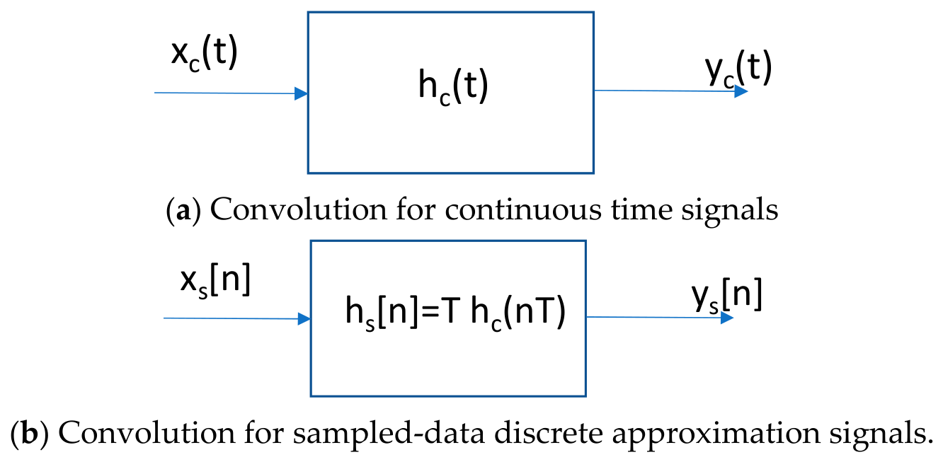
Let $x_c\left(t\right)$, $h_c\left(t\right)$, and $y_c\left(t\right)$ denote the continuous-time input, impulse response, and output, respectively. By definition, the convolution between two functions in time is given by

$$y_c\left(t\right)=x_c\left(t\right)\ast h_c\left(t\right)={\int }_{-\infty }^t{x}_c\left(\tau \right)h_c\left(t-\tau \right)d\tau$$

(21)

This is shown in Figure 2a.

Given a sampling period T, (21) can be discretized

$$y_c\left(nT\right)=x_c\left(nT\right)\ast h_c\left(nT\right)={\displaystyle {\sum }_{k=-\infty }^n}{x}_c\left(kT\right)h_c\left(nT-kT\right)·T$$

(22)

Define the sampled impulse-response sequence

$$h_s\left[n\right]=T{h}_c\left(nT\right).$$

(23)

Then the sampled-data convolution can be written as

$$y_s[n]={\displaystyle {\sum }_{k=-\infty }^n}{x}_s\left[k\right]h_s[n-k],$$

(24)

where $x_s\left[n\right]$ is the sampled input sequence and $y_s\left[n\right]$ is the sampled output sequence. Under this notation, the factor T is carried explicitly by the sampled impulse response $h_s\left[n\right]$. This does not redefine native discrete-time convolution; it only specifies the sampled-data convention used to approximate the continuous-time convolution integral.

Equation (23) ensures that $y_s\left[n\right]$ and $y\left(t\right)$ have similar magnitudes. The discrete time convolution is shown in Figure 2b. Actually, people usually forget about the importance of the factor T in discrete time convolution, resulting in a factor of T difference between continuous time and discrete time convolution results. Books [17,18] related to optics, however, do explicitly take the discretization factor (sampling period) into account to ensure continuous signals have similar magnitudes as the discrete counterparts.

3.4. Explanations of the Issues in Section 2

We can now apply the above material to explain the issues in Section 2. Under the midpoint-consistent sampled convention used here, the sampled step satisfies $u_s\left[0\right]=1/2$.

To address the scaling factor T, we treat one sequence as the sampled impulse response and multiply it by T following the sampled-data interpretation in Figure 2b. With this convention, the resulting discrete calculation is designed to match the sampled continuous-time convolution result as closely as possible. For this reason, we refer to the result below as a midpoint-consistent sampled convolution, rather than a universally corrected discrete convolution. Consequently, the discrete convolution of two step functions should be

$$\begin{array}{cc}\hfill y_s\left[n\right]& =\left(u\left[n\right]-0.5\delta \left[n\right]\right)\ast T(u\left[n\right]-0.5\delta [n\left]\right)\hfill \\ \hfill & =Tu\left[n\right]\ast u\left[n\right]-Tu\left[n\right]+0.25T\delta \left[n\right]\hfill \\ \hfill & =\left(n+1\right)Tu\left[n\right]-Tu\left[n\right]+0.25T\delta \left[n\right]\hfill \\ \hfill & =nTu\left[n\right]+0.25T\delta \left[n\right]\hfill \end{array}$$

(25)

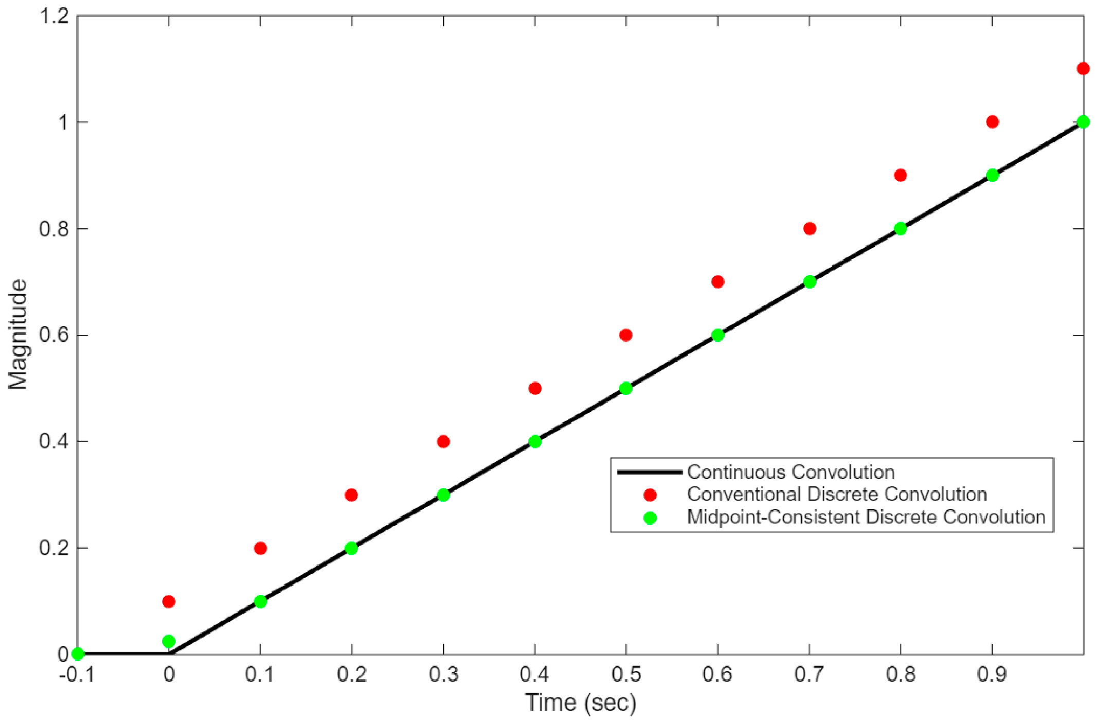
Now we tabulate the various convolution outputs in

Table 2. Comparison of continuous and discrete convolution outputs of two step functions. T = 0.1.

Time (s)	0	0.1	0.2	0.3
Sampling index n	0	1	2	3
Continuous convolution: tu(t)	0	0.1	0.2	0.3
Discrete convolution: $(n+1)u\left[n\right]$	1	2	3	4
Scaled discrete convolution: $(n+1)Tu\left[n\right]$	0.1	0.2	0.3	0.4
Midpoint-consistent sampled convolution: $nTu\left[n\right]+0.25T\delta \left[n\right]$	0.025	0.1	0.2	0.3

. It can be clearly seen that the midpoint-consistent sampled convolution samples (row 6 in Table 2) more closely match the continuous convolution outputs (row 3 in Table 2). To easily compare the various convolution outputs, we also plot them in Figure 3.

Table 3. MAE and NRMSE values for convolution outputs with different sampling periods.

	Sampling Period	T = 0.02 (s)	T = 0.05 (s)	T = 0.1 (s)
Error Metric
MAE	Conventional	0.020	0.05	0.1
	Midpoint-consistent	0.005	0.013	0.025
NRMSE	Conventional	0.034	0.086	0.169
	Midpoint-consistent	0.0012	0.0047	0.0127

also summarizes the maximum absolute error (MAE) and the normalized root-mean-square-error (NRMSE) metrics for three sampling periods. It can be seen that the midpoint-consistent sampled convolutions are much closer to the continuous convolution results.

4. Main Results

4.1. Midpoint-Consistent Sampled Sequence Representations for Continuous Functions

Using the sampled-data convention established in Section 3,

Table 4. Sampled sequences of some well-known continuous functions with discontinuities at t = 0.

Continuous	Fourier	Laplace	Sampled Sequence (Conventional)	Sampled Sequence (Midpoint-Consistent)
$u\left(t\right)$	$\pi \delta \left(\omega \right)+{\displaystyle \frac{1}{j\omega }}$	${\displaystyle \frac{1}{s}}$	$u\left[n\right]$	$u\left[n\right]-0.5\delta \left[n\right]$
$e^{-pt}u\left(t\right),p>0$	${\displaystyle \frac{1}{j\omega +p}}$	${\displaystyle \frac{1}{s+p}}$	$e^{-pnT}u\left[n\right]$	$e^{-pnT}u\left[n\right]-0.5\delta \left[n\right]$
$\mathrm{c}\mathrm{o}\mathrm{s}\left(bt\right)u\left(t\right)$	${\displaystyle \frac{j\omega }{-{\omega }^2+b^2}}+{\displaystyle \frac{\pi }{2}}\left[\delta \left(\omega -b\right)+\delta \left(\omega +b\right)\right]$	${\displaystyle \frac{s}{s^2+b^2}}$	$\cos \left(bnT\right)u\left[n\right]$	$\cos \left(bnT\right)u\left[n\right]-0.5\delta \left[n\right]$
$e^{-at}\mathrm{c}\mathrm{o}\mathrm{s}\left(bt\right)u\left(t\right)$	${\displaystyle \frac{a+j\omega }{{\left(a+j\omega \right)}^2+b^2}}$	${\displaystyle \frac{s+a}{{(s+a)}^2+b^2}}$	$e^{-anT}\cos \left(bnT\right)u\left[n\right]$	$e^{-anT}\cos \left(bnT\right)u\left[n\right]-0.5\delta \left[n\right]$
$x\left(t\right)={\displaystyle \sum _{k=1}^N}{A}_k{e}^{-p_{k}t}u(t)$	$X\left(j\omega \right)={\displaystyle \sum _{k=1}^N}{\displaystyle \frac{A_k}{j\omega +p_k}}$	$X\left(s\right)={\displaystyle \sum _{k=1}^N}{\displaystyle \frac{A_k}{s+p_k}}$	${\displaystyle \sum _{k=1}^N}{A}_k{e}^{-p_{k}nT}u[n]$	${\displaystyle \sum _{k=1}^N}{A}_k{e}^{-p_{k}nT}u[n]-{\displaystyle \sum _{k=1}^N}{\displaystyle \frac{A_k}{2}}\delta [n]$

summarizes midpoint-consistent sampled representations for several functions with jumps at t = 0. The last row assumes that H(s) is strictly proper.

Here, we include the inverse Fourier transform of $\pi \delta \left(\omega \right)+{\displaystyle \frac{1}{j\omega }}$ (second row of Table 4) evaluated at t = 0. The derivations of the rest of the expressions in Table 4 are summarized in the Appendix A, Appendix B, Appendix C, Appendix D and Appendix E.

From [7], the Fourier transform pair for a step function is given by

$$u\left(t\right)\leftrightarrow \pi \delta \left(\omega \right)+{\displaystyle \frac{1}{j\omega }}$$

(26)

If we perform the inverse Fourier transform of $\pi \delta \left(\omega \right)+{\displaystyle \frac{1}{j\omega }}$, we will have

$$u\left(t\right)={\displaystyle \frac{1}{2\pi }}{\int }_{-\infty }^{\infty }\left(\pi \delta \left(\omega \right)+{\displaystyle \frac{1}{j\omega }}\right)e^{j\omega t}d\omega$$

(27)

We are interested in the value of u(0). Setting t = 0 in (26) yields

$$\begin{array}{cc}\hfill u\left(0\right)& ={\displaystyle \frac{1}{2\pi }}{\int }_{-\infty }^{\infty }\left(\pi \delta \left(\omega \right)+{\displaystyle \frac{1}{j\omega }}\right)d\omega \hfill \\ \hfill & ={\displaystyle \frac{1}{2\pi }}{\int }_{-\infty }^{\infty }\left(\pi \delta \left(\omega \right)\right)d\omega +{\displaystyle \frac{1}{2\pi }}{\int }_{-\infty }^{\infty }\left({\displaystyle \frac{1}{j\omega }}\right)d\omega \hfill \end{array}$$

(28)

Note that the first integral involving $\pi \delta \left(\omega \right)$ is 1/2 and the second integral involving ${\displaystyle \frac{1}{j\omega }}$ is zero because ${\displaystyle \frac{1}{j\omega }}$ is an odd function. Hence, when u(t) is represented by the sampled sequence $u_s\left[n\right]$, the midpoint-consistent value is $u_s\left[0\right]=1/2$.

4.2. Midpoint-Consistent Sampled Convolution Formulae

When performing convolution, it is important to distinguish a native discrete-time system from a sampled approximation of a continuous-time system. In the latter case, one sequence plays the role of the sampled impulse response and therefore carries the factor T, while sequences with jump discontinuities may also require midpoint-consistent values at n = 0.

Table 5. Convolution of well-known signals in the continuous and discrete domains. Both conventional and midpoint-consistent formulae are included. Signal $x_c$ is treated as the input and $h_c$ is treated as the system impulse response. Exponential rows apply to both growing and decaying exponentials; the decaying case follows by setting $\lambda =-a,a>0$ (or ${\lambda }_1=-a_i,a_i>0$). For stable impulse-response interpretations, the decaying case is assumed. Note that, in the last row, $x_1\left[n\right]$ and $x_2\left[n\right]$ denote conventional right-continuous samples, so that $x_i\left[0\right]=x_i\left(0^{+}\right),i=1,2$. The midpoint correction is therefore proportional to the jump size $x_i{(0}^{+})-x_i\left(0^{-}\right),i=1,2$.

${\mathit{x}}_{\mathit{c}}\left(\mathit{t}\right)$	${\mathit{h}}_{\mathit{c}}\left(\mathit{t}\right)$	${\mathit{y}}_{\mathit{c}}\left(\mathit{t}\right)={\mathit{x}}_{\mathit{c}}\left(\mathit{t}\right)\ast {\mathit{h}}_{\mathit{c}}\left(\mathit{t}\right)$	${\mathit{x}}_{\mathit{d}}\left[\mathit{n}\right]$ (Conventional)	${\mathit{h}}_{\mathit{d}}\left[\mathit{n}\right]$ (Conventional)	${\mathit{y}}_{\mathit{d}}\left[\mathit{n}\right]$ (Conventional)	${\mathit{x}}_{\mathit{s}}\left[\mathit{n}\right]$ (Midpoint-Consistent Sampled)	${\mathit{h}}_{\mathit{s}}\left[\mathit{n}\right]$ (Midpoint-Consistent Sampled)	${\mathit{y}}_{\mathit{s}}\left[\mathit{n}\right]$ (Midpoint-Consistent Sampled)
$u\left(t\right)$	$u\left(t\right)$	$tu\left(t\right)$	$u\left[n\right]$	$Tu\left[n\right]$	$(n+1)Tu\left[n\right]$	$u\left[n\right]-0.5\delta \left[n\right]$	$Tu\left[n\right]-0.5T\delta \left[n\right]$	$nTu\left[n\right]$ + 0.25$T\delta \left[n\right]$
$u\left(t\right)$	$tu\left(t\right)$	$0.5t^{2}u\left(t\right)$	$u\left[n\right]$	$T^{2}nu[n]$	$0.5n(n+1)T^{2}u\left[n\right]$	$u\left[n\right]-0.5\delta \left[n\right]$	$n{T}^{2}u\left[n\right]$	$0.5n^2{T}^{2}u\left[n\right]$
$u\left(t\right)$	$e^{\lambda t}u\left(t\right)$	${\displaystyle \frac{1-e^{\lambda t}}{-\lambda }}u(t)$	$u\left[n\right]$	${Te}^{\lambda nT}u[n]$	$T\left[{\displaystyle \frac{1-e^{\lambda (n+1)T}}{1-e^{\lambda T}}}\right]u[n]$	$u\left[n\right]-0.5\delta \left[n\right]$	${Te}^{\lambda nT}u[n]-0.5T\delta [n]$	T${\displaystyle \frac{1+e^{\lambda T}}{2}}\left[{\displaystyle \frac{1-e^{\lambda nT}}{1-e^{\lambda T}}}\right]u\left[n\right]+0.25T\delta [n]$
$e^{{\lambda }_{1}t}u\left(t\right)$	$e^{{\lambda }_{2}t}u\left(t\right)$	${\displaystyle \frac{e^{{\lambda }_{1}t}-e^{{\lambda }_{2}t}}{{\lambda }_1-{\lambda }_2}}u(t)$	$e^{{\lambda }_{1}nT}u[n]$	${Te}^{{\lambda }_{2}nT}u[n]$	$\left[{\displaystyle \frac{e^{{\lambda }_1(n+1)T}-e^{{\lambda }_2(n+1)T}}{e^{{\lambda }_{1}T}-e^{{\lambda }_{2}T}}}\right]Tu[n]$	$e^{{\lambda }_{1}nT}u[n]-0.5\delta [n]$	${Te}^{{\lambda }_{2}nT}u[n]-0.5T\delta [n]$	$T{\displaystyle \frac{e^{{\lambda }_{1}T}+e^{{\lambda }_{2}T}}{2}}\left[{\displaystyle \frac{e^{{\lambda }_{1}nT}-e^{{\lambda }_{2}nT}}{e^{{\lambda }_{1}T}-e^{{\lambda }_{2}T}}}\right]u\left[n\right]+0.25T\delta [n]$
$x_1$(t)	$x_2$(t)	$x_1\left(\mathrm{t}\right)\ast x_2\left(\mathrm{t}\right)$	$x_1\left[\mathrm{n}\right]$	$T{x}_2\left[\mathrm{n}\right]$	$x_1\left[\mathrm{n}\right]\ast T{x}_2\left[n\right]$	$x_1[n]-0.5(x_1\left(0^{+}\right)-x_1\left(0^{-}\right))\delta [n]$	$T{x}_2[n]-0.5T(x_2\left(0^{+}\right)-x_2\left(0^{-}\right))\delta [n]$	${Tx}_1\left[n\right]\ast x_2\left[n\right]-0.5T\left(x_2{(0}^{+})-x_2(0^{-})\right)x_1\left[n\right]-0.5T\left(x_1{(0}^{+})-x_1(0^{-})\right)x_2\left[n\right]+0.25T\left(x_1{(0}^{+}\right)-x_1\left(0^{-}\right)\left)\right(x_2{(0}^{+})-x_2(0^{-}\left)\right)\delta [n]$

summarizes the continuous-time formulae, the conventional discrete formulae, and the midpoint-consistent sampled formulae under this interpretation.

For the second row in Table 5, we already derived the convolution formulae in Section 3.4. That is, the last column in row 2 is basically Equation (25). Now, we will derive those formulae in row 3 to row 6.

• Derivation of the Formula in Row 3 of Last Column in Table 5

The convolution between $x_s\left[n\right]$ and $h_s\left[n\right]$ is given by

$$\begin{array}{cc}\hfill y_s\left[n\right]& =\left(u\left[n\right]-0.5\delta \left[n\right]\right)\ast \left(n{T}^{2}u\left[n\right]\right)\hfill \\ \hfill & =T^{2}u\left[n\right]\ast nu\left[n\right]-0.5T^{2}u\left[n\right]\hfill \\ \hfill & =0.5n\left(n+1\right)T^{2}u\left[n\right]-0.5T^{2}u\left[n\right]\hfill \\ \hfill & =0.5n^2{T}^{2}u\left[n\right]\hfill \end{array}$$

(29)

• Derivation of the Formula in Row 4 of Last Column in Table 5

Here, the midpoint-consistent convolution expression is given by

$$\begin{array}{cc}\hfill y_s\left[n\right]& =\left(u\left[n\right]-0.5\delta \left[n\right]\right)\ast ({Te}^{\lambda nT}u\left[n\right]-0.5T\delta \left[n\right])\hfill \\ \hfill & ={Te}^{\lambda nT}u\left[n\right]\ast u\left[n\right]-0.5{Te}^{\lambda nT}u\left[n\right]+0.25T\delta \left[n\right]\hfill \\ \hfill & =T\left[{\displaystyle \frac{1-e^{\lambda (n+1)T}}{1-e^{\lambda T}}}\right]u[n]-0.5{Te}^{\lambda nT}u\left[n\right]+0.25T\delta \left[n\right]\hfill \\ \hfill & =T{\displaystyle \frac{1+e^{\lambda T}}{2}}\left[{\displaystyle \frac{1-e^{\lambda nT}}{1-e^{\lambda T}}}\right]u\left[n\right]+0.25T\delta \left[n\right]\hfill \end{array}$$

(30)

• Derivation of the Formula in Row 5 of Last Column in Table 5

The midpoint-consistent convolution is given by

$$\begin{array}{cc}\hfill y_s\left[n\right]& =\left(e^{{\lambda }_{1}nT}u\left[n\right]-0.5\delta \left[n\right]\right)\ast \left({Te}^{{\lambda }_{2}nT}u\right[n]-0.5T\delta [n\left]\right)\hfill \\ \hfill & ={Te}^{{\lambda }_{2}nT}u\left[n\right]\ast e^{{\lambda }_{1}nT}u\left[n\right]-0.5T{e}^{{\lambda }_{1}nT}u\left[n\right]-0.5T{e}^{{\lambda }_{2}nT}u\left[n\right]+0.25T\delta \left[n\right]\hfill \\ \hfill & =\left[{\displaystyle \frac{e^{{\lambda }_1(n+1)T}-e^{{\lambda }_2(n+1)T}}{e^{{\lambda }_{1}T}-e^{{\lambda }_{2}T}}}\right]Tu\left[n\right]-0.5T{e}^{{\lambda }_{1}nT}u\left[n\right]-0.5T{e}^{{\lambda }_{2}nT}u\left[n\right]+0.25T\delta [n]\hfill \\ \hfill & =T{\displaystyle \frac{e^{{\lambda }_{1}T}+e^{{\lambda }_{2}T}}{2}}\left[{\displaystyle \frac{e^{{\lambda }_{1}nT}-e^{{\lambda }_{2}nT}}{e^{{\lambda }_{1}T}-e^{{\lambda }_{2}T}}}\right]u\left[n\right]+0.25T\delta [n]\hfill \end{array}$$

(31)

• Derivations of the Formula in Row 6 of Last Column in Table 5

At n = 0,

$$x_i\left[0\right]=x_i\left(0^{+}\right),\hspace{1em}\hspace{1em}\hspace{1em}\hspace{1em}i=1,2.$$

Then the midpoint-consistent sampled versions should be

$$x_{1,s}\left[n\right]=x_1\left[n\right]-0.5\left(x_1{(0}^{+}\right)-x_1\left(0^{-}\right)\left)\delta \right[n],$$

and

$$h_s\left[n\right]=T{x}_2\left[n\right]-0.5T\left(x_2{(0}^{+}\right)-x_2\left(0^{-}\right)\left)\delta \right[n].$$

The midpoint-consistent convolution is given by

$$\begin{array}{cc}\hfill y_s\left[n\right]& ={(x}_1\left[n\right]-0.5\left(x_1{(0}^{+}\right)-x_1\left(0^{-}\right)\left)\delta \right[n\left]\right)\ast T{(x}_2\left[n\right]-0.5(x_2\left[0^{+}\right]-x_2[0^{-}\left]\right)\delta \left[n\right])\hfill \\ \hfill & ={Tx}_1\left[n\right]\ast x_2\left[n\right]-0.5T\left(x_2{(0}^{+})-x_2(0^{-})\right)x_1\left[n\right]-0.5T\left(x_1{(0}^{+})-x_1(0^{-})\right)x_2\left[n\right]+0.25T\left(x_1{(0}^{+}\right)-x_1\left(0^{-}\right)\left)\right(x_2{(0}^{+})-x_2(0^{-}\left)\right)\delta \left[n\right]\hfill \end{array}$$

(32)

5. Experimental Results

Here, we include a few examples to compare the conventional and midpoint-consistent formulae in Table 5.

Example 1: Convolution of one step and one ramp function.

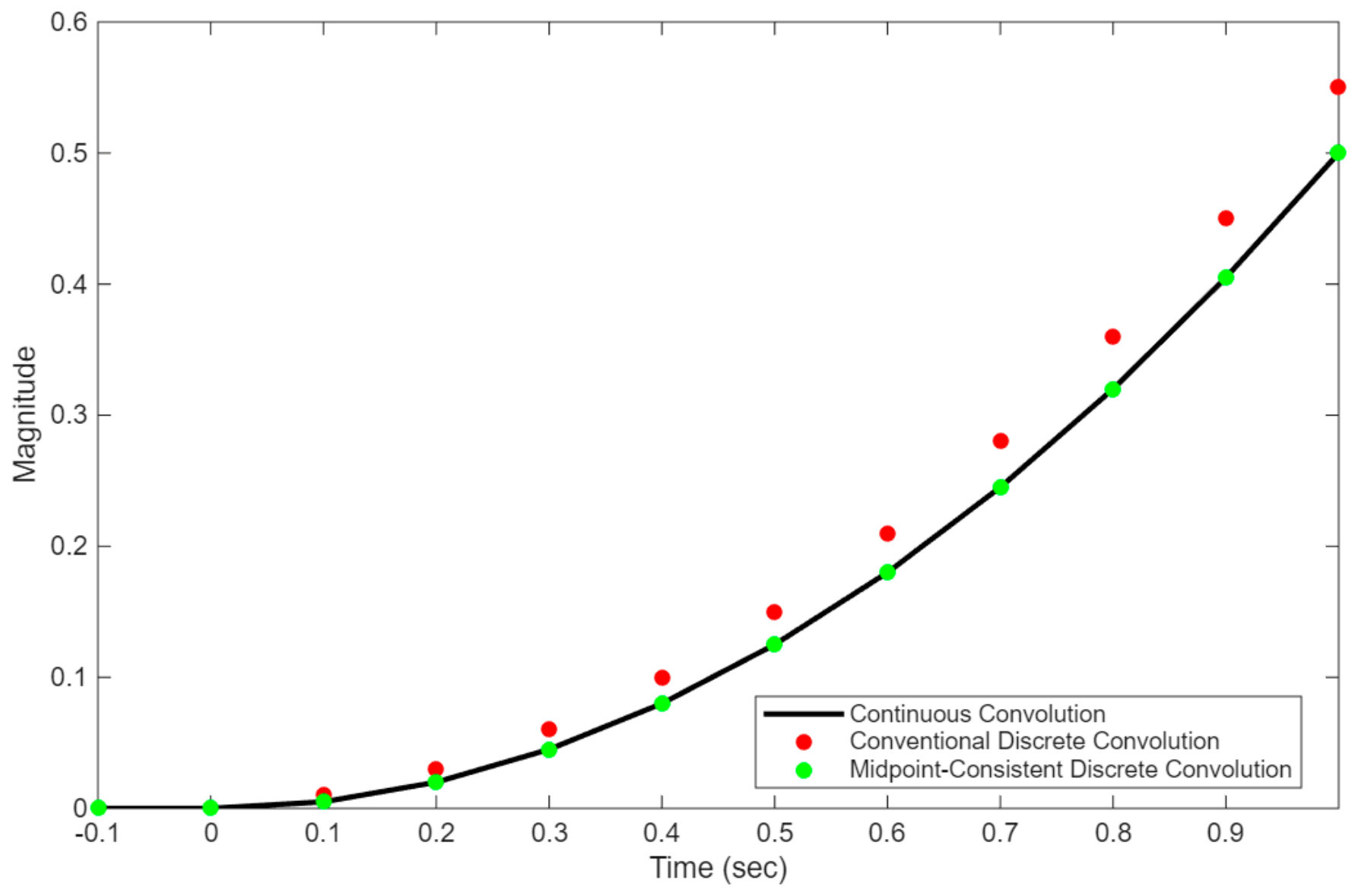
The corresponding formulae for the convolution of one step and one ramp function are shown in row 3 of Table 5.

Table 6. Various convolution outputs between a unit step and a ramp. T = 0.1.

Time (s)	0	0.1	0.2	0.3
n	0	1	2	3
0.5$t^2$u(t)	0	0.005	0.02	0.045
$0.5n(n+1)T^{2}u\left[n\right]$	0	0.01	0.03	0.06
$0.5n^2{T}^{2}u\left[n\right]$	0	0.005	0.02	0.045

compares the various convolution results for a few samples. One can see that the continuous and midpoint-consistent sampled convolution results are exactly the same. Figure 4 also plots the three convolution outputs up to 1 s. It can be seen that the gap between the conventional discrete and the midpoint-consistent sampled convolution results grows bigger as time increases. This demonstrates the importance of using a sampled-data formulation consistent with the continuous-time model under the stated assumptions.

Table 7. MAE and NRMSE values for convolution outputs with different sampling periods.

	Sampling Period	T = 0.02 (s)	T = 0.05 (s)	T = 0.1 (s)
Error Metric
MAE	Conventional	0.010	0.025	0.05
	Midpoint-consistent	0.000	0.000	0.000
NRMSE	Conventional	0.026	0.063	0.123
	Midpoint-consistent	0.000	0.000	0.000

also summarizes the MAE and the NRMSE metrics for three sampling periods. The midpoint-consistent sampled convolution outputs are closely matched to the continuous convolution results.

Example 2: Convolution between a step and an exponential function.

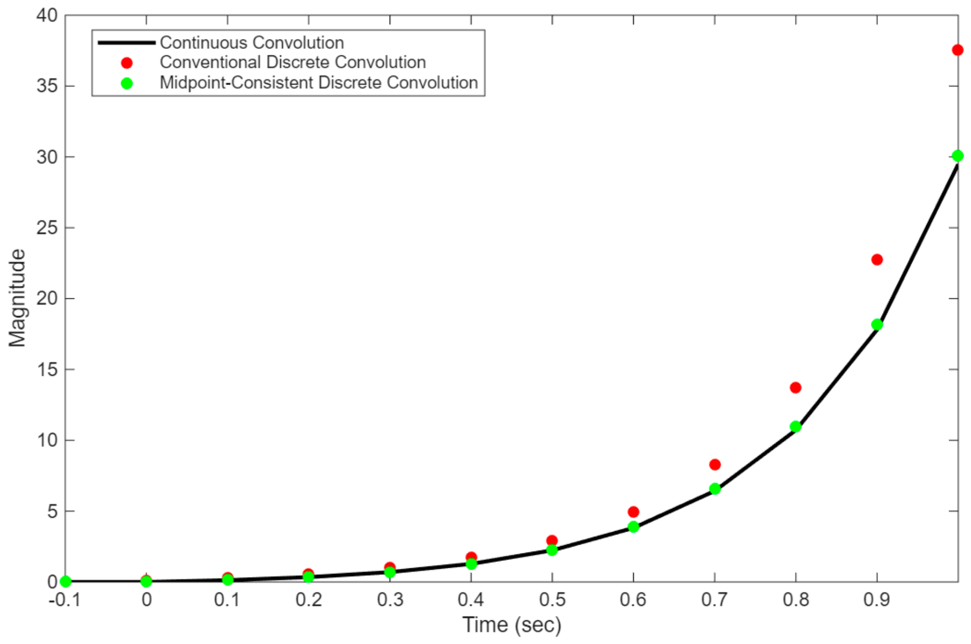
Here, we want to show the convolution between $u\left(t\right)$ and $e^{\lambda t}u\left(t\right)$ with $\lambda$ = 5. The corresponding formulae are shown in row 4 of Table 5. The sampling interval T = 0.1 s. Figure 5 shows the convolution outputs. We can see that for this growing-exponential example, the absolute difference increases with n.

Table 8. Various convolution outputs between a unit step and an exponential function. T = 0.1.

Time (s)	0	0.1	0.2	0.3
n	0	1	2	3
${\displaystyle \frac{1-e^{\lambda t}}{-\lambda }}u(t)$	0	0.1297	0.3437	0.6963
$T\left[{\displaystyle \frac{1-e^{\lambda (n+1)T}}{1-e^{\lambda T}}}\right]u[n]$	0.1	0.2649	0.5367	0.9849
T${\displaystyle \frac{1+e^{\lambda T}}{2}}\left[{\displaystyle \frac{1-e^{\lambda nT}}{1-e^{\lambda T}}}\right]u\left[n\right]+0.25T\delta [n]$	0.025	0.1324	0.3508	0.7108

contains results from four time instants. At t = 1 or n =10, the difference between the conventional discrete response $y_d\left[n\right]$ and midpoint-consistent sampled responses $y_s\left[n\right]$ is about 8.08 for the reported example, which is non-negligible. This large difference is simply caused by the small discontinuity at t = 0.

Table 9. MAE and NRMSE values for convolution outputs with different sampling periods.

	Sampling Period	T = 0.02 (s)	T = 0.05 (s)	T = 0.1 (s)
Error Metric
MAE	Conventional	1.519	3.889	8.082
	Midpoint-consistent	0.025	0.153	0.612
NRMSE	Conventional	0.052	0.133	0.276
	Midpoint-consistent	0.00084	0.0052	0.021

also summarizes the maximum absolute error (MAE) and the normalized root-mean-square-error (NRMSE) metrics for three sampling periods. The same trend is observed in Table 9: the midpoint-consistent sampled result has substantially smaller MAE and NRMSE than the conventional discrete result.

Example 3: Convolution between two exponential functions.

This is the convolution between two exponential functions: $e^{{\lambda }_{1}t}u\left(t\right)$ and $e^{{\lambda }_{2}t}u\left(t\right)$ with ${\lambda }_1=5$ and ${\lambda }_2=3$. From row 5 of Table 5, the convolution of the continuous functions gives

$$y\left(t\right)={\displaystyle \frac{e^{{\lambda }_{1}t}-e^{{\lambda }_{2}t}}{{\lambda }_1-{\lambda }_2}}u(t).$$

Also from Table 5, the conventional discrete convolution output is

$$y\left[n\right]=\left[{\displaystyle \frac{e^{{\lambda }_1(n+1)T}-e^{{\lambda }_2(n+1)T}}{e^{{\lambda }_{1}T}-e^{{\lambda }_{2}T}}}\right]Tu[n]$$

Finally, from Table 5, the midpoint-consistent sampled convolution output is

$$y(nT)=T{\displaystyle \frac{e^{{\lambda }_{1}T}+e^{{\lambda }_{2}T}}{2}}\left[{\displaystyle \frac{e^{{\lambda }_{1}nT}-e^{{\lambda }_{2}nT}}{e^{{\lambda }_{1}T}-e^{{\lambda }_{2}T}}}\right]u\left[n\right]+0.25T\delta [n].$$

Table 10. Various convolution outputs between two exponential functions. T = 0.1.

Time (s)	0	0.1	0.2	0.3
n	0	1	2	3
${\displaystyle \frac{e^{{\lambda }_{1}t}-e^{{\lambda }_{2}t}}{{\lambda }_1-{\lambda }_2}}u(t)$	0	0.1494	0.4481	1.0110
$\left[{\displaystyle \frac{e^{{\lambda }_1(n+1)T}-e^{{\lambda }_2(n+1)T}}{e^{{\lambda }_{1}T}-e^{{\lambda }_{2}T}}}\right]Tu[n]$	0.1	0.2999	0.6766	1.3615
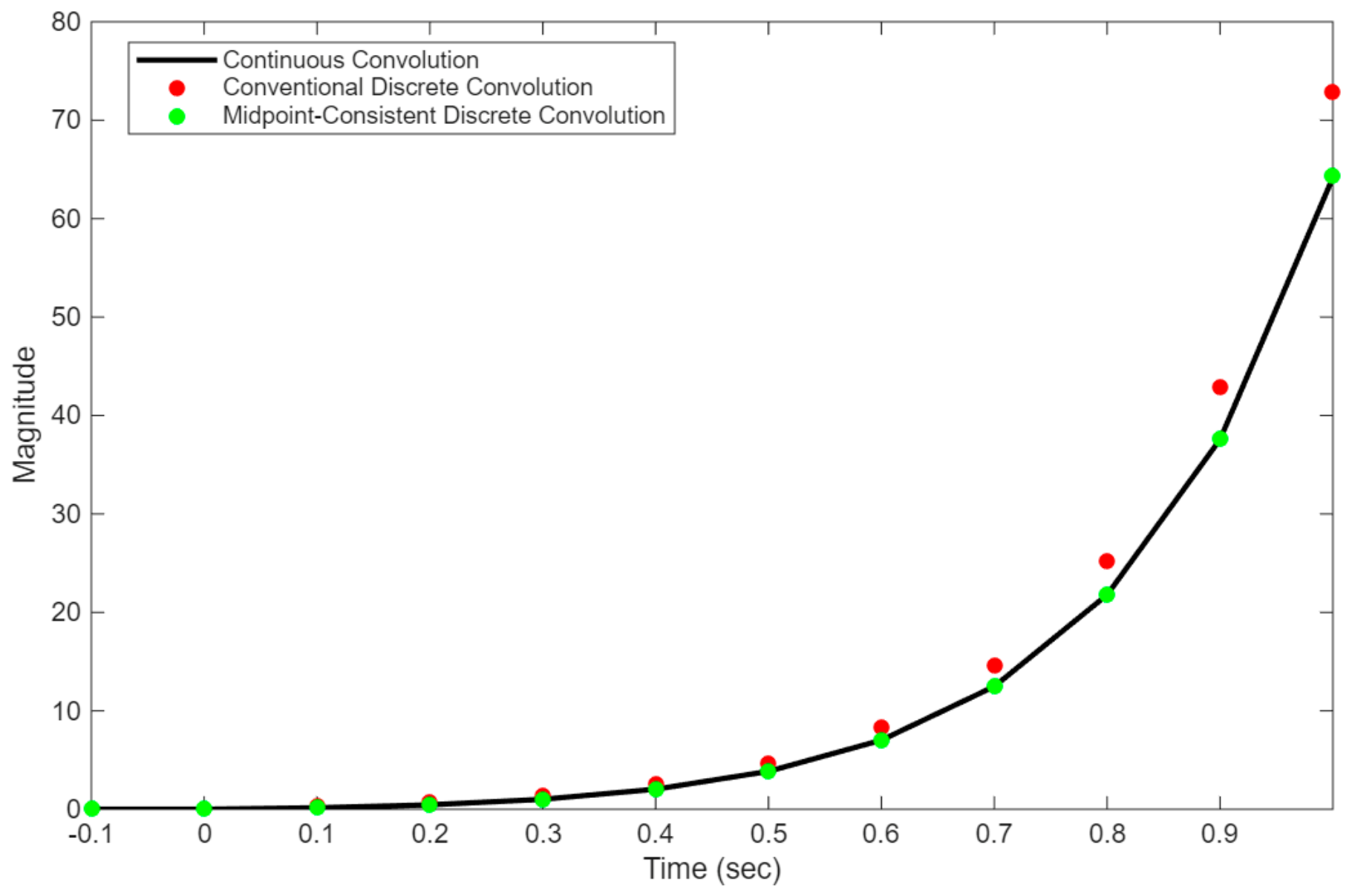
$T{\displaystyle \frac{e^{{\lambda }_{1}T}+e^{{\lambda }_{2}T}}{2}}\left[{\displaystyle \frac{e^{{\lambda }_{1}nT}-e^{{\lambda }_{2}nT}}{e^{{\lambda }_{1}T}-e^{{\lambda }_{2}T}}}\right]u\left[n\right]+0.25T\delta [n]$	0.025	0.1499	0.4496	1.0144

tabulates a few samples for the various convolution outputs. Figure 6 also shows those convolution outputs. One can see that as time increases, the difference between the discrete and continuous outputs grows progressively larger. For instance, at t = 1 s, the difference is close to 10.

Table 11. MAE and NRMSE values for convolution outputs with different sampling periods.

	Sampling Period	T = 0.02 (s)	T = 0.05 (s)	T = 0.1 (s)
Error Metric
MAE	Conventional	1.694	4.266	8.639
	Midpoint-consistent	0.0086	0.053	0.214
NRMSE	Conventional	0.028	0.070	0.140
	Midpoint-consistent	0.00014	0.00084	0.0033

also summarizes the MAE and the NRMSE metrics for three sampling periods. The midpoint-consistent sampled convolution outputs have approximately two-order of magnitude smaller errors in MAE and NRMSE as compared to the conventional convolution outputs.

Example 4: Step response of a bandpass filter.

The continuous step input is $u\left(t\right)$, the conventional native discrete-time step sequence is $u_d\left[n\right]$, and the midpoint-consistent sampled sequence is $u_s\left[n\right]=u_d\left[n\right]-0.5\delta \left[n\right]$. For a given bandpass filter

$$H_{bp}\left(s\right)={\displaystyle \frac{2\left(2\right)s}{{(s+2)}^2+{10}^2}},$$

its continuous impulse response is given by

$$h_{bp}\left(t\right)=4e^{-2t}\left(\cos \left(10t\right)-0.2\mathrm{s}\mathrm{i}\mathrm{n}\left(10t\right)\right).$$

For a sampling period of T, the conventional discrete impulse response sequence is given by

$$h_d\left[n\right]=T{h}_{bp}\left(nT\right)$$

Since there is a discontinuity from 0 to 4 at t = 0 for the bandpass filter, a correction term of 2 is needed for the midpoint-consistent impulse response sequence $h_s\left[n\right]$. Hence, the expression for the midpoint-consistent sampled impulse response sequence of the filter is given by

$$h_s\left[n\right]=T(h_{bp}\left(nT\right)-2\delta \left[n\right])).$$

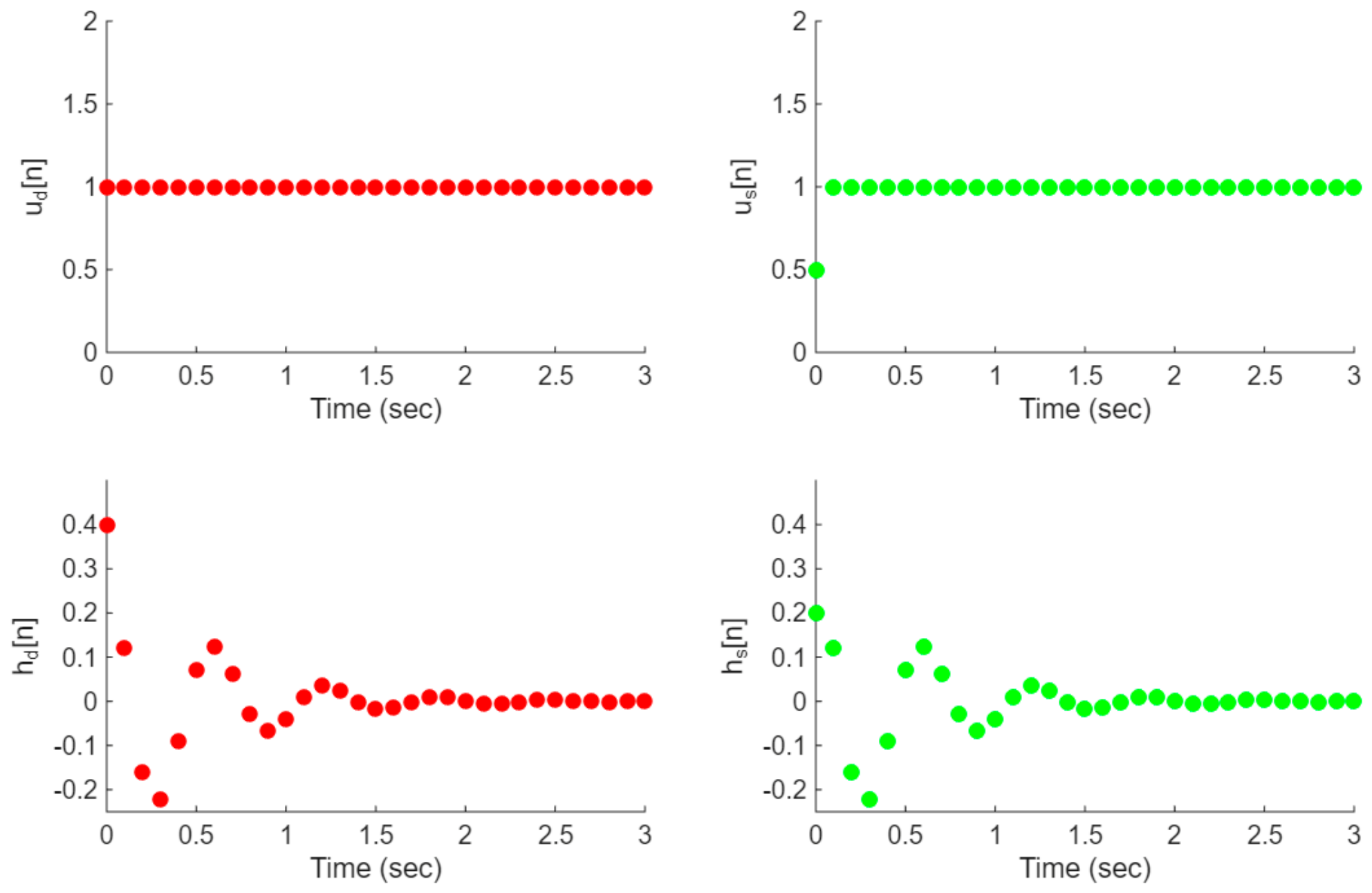
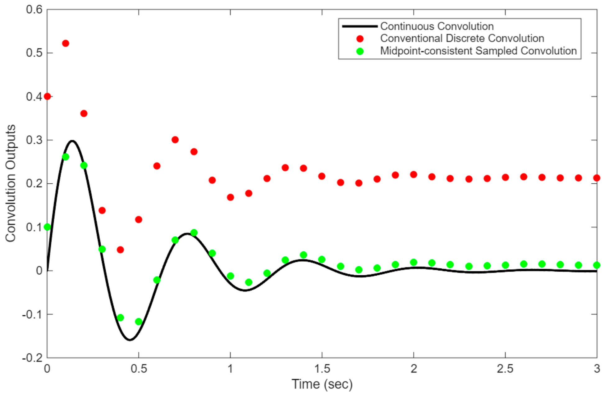
The left column of Figure 7 shows the conventional native discrete-time step function and the scaled discrete impulse response of the bandpass filter. The right column of Figure 7 shows the midpoint-consistent sampled unit step function and the scaled sampled impulse response of the filter. It can be clearly seen that the differences between the left and right columns of Figure 7 are at n = 0. The impact of these small differences is actually quite substantial, which can be seen in Figure 8. We can clearly see that the conventional discrete convolution response of the bandpass filter is quite different from that of the continuous step response. After adding the small correction at n = 0, the midpoint-consistent sampled step response is almost overlapping the continuous step response.

To further quantify the performance improvement of using the midpoint-consistent sampled sequences, we compute the errors between the conventional discrete convolution and the continuous convolution, and also the errors between the midpoint-consistent sampled convolution and the continuous convolution.

Table 12. MAE and NRMSE values for convolution outputs with different sampling periods.

	Sampling Period	T = 0.02 (s)	T = 0.05 (s)	T = 0.1 (s)
Error Metric
MAE	Conventional	0.079	0.199	0.399
	Midpoint-consistent	0.019	0.049	0.099
NRMSE	Conventional	0.520	1.336	2.808
	Midpoint-consistent	0.021	0.091	0.292

tabulates the maximum absolute error (MAE) and normalized root-mean-square-error (NRMSE) values for the two error sequences. There are three sampling periods: T = 0.02 s, T = 0.05 s, and T = 0.1 s. One can see that the performance gain from using the midpoint-consistent sampled sequences is substantial because an order of magnitude improvement can be seen in the NRMSE values.

6. Conclusions

Differences between continuous-time convolution outputs and their sampled discrete counterparts can arise for two distinct reasons: the sampling-period scaling used in approximating the continuous convolution integral, and the treatment of signals that are discontinuous at the sampling instant. In this paper, we revisited these issues and clarified their relationship. Although the midpoint value at a jump discontinuity is a classical result from Fourier analysis and distribution theory, we showed how this result can be used systematically to construct midpoint-consistent sampled sequence representations. From this sampled-data interpretation, the corresponding convolution formulae acquire small but explicit modifications. We also stressed that these formulae are intended for sampled continuous-time signals at discontinuities and are not meant to replace standard native discrete-time conventions used in digital signal processing. The examples show that, when T is not negligibly small and a discontinuity occurs at the sampling instant, the midpoint-consistent sampled formulae match the sampled continuous-time results more closely than the conventional formulae.

References

1. Cooley, J.W.; Tukey, J.W. An algorithm for the machine calculation of complex Fourier series. Math. Comput. 1965, 19, 297–301. [Google Scholar] [CrossRef]
2. Ahmed, N.; Natarajan, T.; Rao, K.R. Discrete Cosine Transform. IEEE Trans. Comput. 1974, C-23, 90–93. [Google Scholar] [CrossRef]
3. Kwan, C.; Ho, K.C.; Mei, G.; Li, Y.; Ren, Z.; Xu, R.; Zhang, Y.; Lao, D.; Stevenson, M.; Stanford, V.; et al. An Automated Acoustic System to Monitor and Classify Birds. EURASIP J. Adv. Signal Process. 2006, 2006, 096706. [Google Scholar] [CrossRef]
4. Chan, W.; Jaitly, N.; Le, Q.; Vinyals, O. Listen, attend and spell: A neural network for large vocabulary conversational speech recognition. In Proceedings of the 2016 IEEE International Conference on Acoustics, Speech and Signal Processing (ICASSP), Shanghai, China, 20–25 March 2016; pp. 4960–4964. [Google Scholar]
5. Ugail, H. Deep face recognition using full and partial face images. In Advanced Methods and Deep Learning in Computer; Elsevier: Amsterdam, The Netherlands, 2022. [Google Scholar]
6. Dao, M.; Kwan, C.; Ayhan, B.; Tran, T.D. Burn scar detection using cloudy MODIS images via low-rank and sparsity-based models. In Proceedings of the 2016 IEEE Global Conference on Signal and Information Processing (GlobalSIP), Washington, DC, USA, 7–9 December 2016; pp. 177–181. [Google Scholar]
7. Lathi, B.P.; Green, R. Linear Systems and Signals, 3rd ed.; Oxford University Press: Oxford, UK, 2018. [Google Scholar]
8. Oppenheim, A.V.; Schafer, R.W.; Buck, J.R. Discrete-Time Signal Processing, 3rd ed.; Pearson/Prentice Hall: Upper Saddle River, NJ, USA, 2010. [Google Scholar]
9. Oppenheim, A.V.; Willsky, A.S.; Nawab, S.H. Signals and Systems, 2nd ed.; Prentice Hall: Upper Saddle River, NJ, USA, 1997. [Google Scholar]
10. Proakis, J.; Manolakis, D.G. Digital Signal Processing, 5th ed.; Pearson: London, UK, 2021. [Google Scholar]
11. Lyons, R.G. Understanding Digital Signal Processing, 3rd ed.; Prentice Hall: Hoboken, NJ, USA, 2011. [Google Scholar]
12. Åström, K.J.; Wittenmark, B. Computer-Controlled Systems: Theory and Design, 3rd ed.; Prentice Hall: Upper Saddle River, NJ, USA, 1997. [Google Scholar]
13. Franklin, G.F.; Powell, J.D.; Workman, M.L. Digital Control of Dynamic Systems, 3rd ed.; Addison-Wesley: Reading, MA, USA, 1998. [Google Scholar]
14. Chen, T.; Francis, B.A. Optimal Sampled-Data Control Systems; Springer: London, UK, 1995. [Google Scholar]
15. Jackson, L.B. A correction to impulse invariance. In IEEE Signal Processing Letters; IEEE: New York, NY, USA, 2000; Volume 7, pp. 273–275. [Google Scholar] [CrossRef]
16. Papoulis, A. The Fourier Integral and Its Applications; McGraw-Hill: New York, NY, USA, 1962. [Google Scholar]
17. Voelz, D.G. Computational Fourier Optics: A MATLAB Tutorial; SPIE Press: Bellingham, WA, USA, 2011. [Google Scholar]
18. Schmidt, J.D. Numerical Simulation of Optical Wave Propagation with Examples in MATLAB®; SPIE Press: Bellingham, WA, USA, 2010. [Google Scholar] [CrossRef]
19. Kwan, C.; Ferguson, H. A Fresh Revisit of the Issues and Improvements of Impulse Invariance Filter Design for Infinite Impulse Response Filters. Electronics 2024, 13, 3753. [Google Scholar] [CrossRef]
Figure 1. Comparison of convolution responses. There is a constant difference between the continuous and the scaled discrete convolution results. T = 0.1.
Electronics 15 02962 g001
Figure 2. Continuous-time convolution integral (a) and sampled-data discrete approximation (b) used in this paper.
Electronics 15 02962 g002
Figure 3. Comparison of convolution responses between two unit-step functions. The midpoint-consistent sampled convolution results overlap with the sampled continuous convolution results except a small difference at t = 0. T = 0.1.
Electronics 15 02962 g003
Figure 4. Comparison of convolution responses. The continuous convolution output is 0.5 t 2 u(t). T = 0.1.
Electronics 15 02962 g004
Figure 5. Comparison of convolution responses between a unit step and an exponential function. T = 0.1.
Electronics 15 02962 g005
Figure 6. Comparison of convolution responses between two exponential functions. T = 0.1.
Electronics 15 02962 g006
Figure 7. Left column (red): Conventional discrete sequences. Right column (green): Midpoint-consistent sampled sequences. Top: Input step function; bottom: Scaled discrete impulse response. T = 0.1 s.
Electronics 15 02962 g007
Figure 8. Convolution of a unit step function with a bandpass filter. T = 0.1 s.
Electronics 15 02962 g008