An Efficient Two-Stage Method for Correcting 3-D Positioning Errors of the Measuring Probe in a Non-Redundant Spherical Scan

Abstract

A robust procedure for compensating for inaccuracies caused by 3-D positioning errors in the measurement of the near-field (NF) data required by the non-redundant (NR) spherical near-to-far-field (NtFF) transformations for long antennas is presented in this article. These errors may arise from hardware defects and positioners’ controlling inaccuracies, which may cause the probe to deviate from the intended spherical scan surface and prevent it from reaching the NR sampling points required by either of the two NR representations for long antennas. To account for these errors, the method proceeds through two steps. The first step, called spherical wave correction, compensates for the phase shifts due to radial displacements from the intended scanning sphere. As a result of this correction, the NF samples belong to the intended scanning sphere, but at points different from those required by the adopted NR representation, thus impairing the subsequent NF reconstruction via the optimal sampling interpolation (OSI) algorithm. Such an algorithm enables one to efficiently build the iterative scheme used in the second step, which makes it possible to effectively retrieve the NF samples at the prescribed NR positions. Test results are shown to numerically validate the capability of the developed two-step compensation technique to correct even significant and pessimistic 3-D positioning errors affecting the collection of the NF data.

1. Introduction

Near-field (NF) antenna measurements [1,2,3,4,5,6,7,8,9,10] are nowadays a standard practice for researchers or technicians, since they allow for an accurate characterization of an antenna under test (AUT) via near-to-far-field (NtFF) transformation techniques. This approach is extremely useful when the dimensions of an anechoic chamber do not guarantee to meet the FF requirements.

The classical approach to the NtFF transformation is based on the modal expansion method. According to such a method, the electromagnetic (EM) field radiated by the antenna is expanded into a complete set of solutions to the vector wave equation, such as planar, cylindrical, or spherical waves. As a consequence, planar, cylindrical, and spherical geometries are the primary standards for antenna testing, although they offer different trade-offs. The former two are prone to loss of accuracy in the NF and FF reconstruction due to truncated measurement surfaces, whilst spherical NF (SNF) measurements [11,12,13,14,15,16,17,18,19,20,21,22,23,24,25,26,27,28,29,30,31,32,33,34,35] offer higher accuracy, since the scanning surface surrounds the AUT, thus eliminating such a drawback. In any case, the classical NtFF transformation [16] often demands an unfeasible number of NF samples for large antennas. To address this issue and minimize data requirements, modern non-redundant (NR) sampling techniques [10,36] have been developed. As a matter of fact, by leveraging the spatially band-limited feature of EM fields [37], these techniques are capable of reducing the amount of required NF data to a number close to that of the degrees of freedom of the EM field [38,39], without any accuracy loss. To properly apply these techniques, it is required, as a priori information, to model the AUT by a convex surface exhibiting a rotational symmetry. The basic principle to get a really NR representation upon any regular surface with the same symmetry is that the more closely the modeling surface fits the actual AUT geometry, the fewer amount of samples are required to represent its radiated EM field. An optimal sampling interpolation (OSI) expansion is then applied to retrieve the input NF data required for the standard spherical NtFF transformation [16]. Consequently, the NR spherical NtFF transformations [25,26] significantly decrease acquisition time while maintaining high precision. These last ones adopt prolate spheroids or rounded cylinders and oblate spheroids or double bowls for getting the best fitting of long and quasi-planar AUTs, respectively.

Other NtFF spherical transformations aiming to reduce the amount of necessary NF data are those exploiting the adaptive sampling [27] or the compressed sensing [30,31,32,33].

The reliability of the NtFF transformations relies heavily on precise probe positioning at the sampling points set by the utilized sampling representation. However, hardware limitations, such as the mechanical tolerances of arc systems, stepper motor resolution, and the imperfections inherent in robotic arms, inevitably cause deviations from the ideal sampling grid. These 3-D positioning errors manifest as both radial shifts from the intended measurement sphere and 2-D tangential misalignments along the sampling arrangement. While these deviations can be evaluated using laser interferometry, leaving them uncorrected significantly degrades the reconstructed FF pattern. Although matrix-based correction methods [40,41,42] exist for the NtFF transformations with the conventional planar and spherical scans, they cannot be certainly applicable to restore the NR samples when they are affected by 3-D positioning errors, since the indispensable use of OSI intrinsically requires the samples to lie on the acquisition surface.

This paper presents a novel two-step technique designed to effectively compensate for 3-D probe position errors within the NR spherical NtFF transformations [25,26], specifically tailored for long AUTs. This method extends previous approaches successfully applied to the NR NtFF transformations with planar [43] and cylindrical [44] scanning geometries, as well as those with spherical scans tailored for quasi-planar AUTs [45].

The proposed technique operates in two steps:

• Spherical wave correction (SWC): This phase correction procedure compensates for radial displacements of the samples relative to the intended measurement sphere. It works analogously to the k-correction and cylindrical wave correction (CWC) used in planar [43,46] and cylindrical scan [44] geometries, respectively.
• NR NF sample reconstruction through an iterative algorithm: this well-established algorithm [47,48] is used to accurately recover the NF data at their exact positions on the devised NR grid, thus correcting the remaining 2-D errors.

Once the 3-D errors have been compensated, the retrieved NF samples are interpolated by an OSI algorithm to get the input data necessary for the standard spherical NtFF transformation [16].

The feasibility and reliability of the developed technique for both the NtFF transformations for long AUTs is assessed by numerical tests, which demonstrates its capability to precisely restore the NR NF samples even in measuring environments characterized by realistic or even severe positioning errors.

The paper organization is outlined in the following for readers’ convenience. The development of the NR sampling representation of the voltage detected by a non-directive probe over the spherical scanning surface, relying on the use of either the prolate spheroid or rounded cylinder to shape a long AUT, and the related OSI algorithm to get the voltage value everywhere on the sphere are summarized in Section 2. Section 3 formalizes the problem of 3-D probe position errors correction and provides a comprehensive description of the developed two-stage technique to correct them. Test results, assessing the performance and the reliability of the technique, are presented and discussed in the following section. At last, concluding remarks are collected in Section 5.

2. NR Sampling Arrangement over a Sphere

For the reader’s convenience, this section outlines the key steps for efficiently obtaining the NR sampling arrangement of the sampling points, where the measuring probe with non-directive characteristics is driven by the positioner controllers of a SNF facility, and the related 2-D OSI formula. The development relies on the NR sampling representations of EM fields [10,36], specifically optimized for long AUTs.

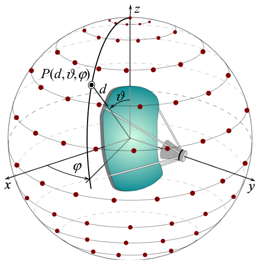
Figure 1 shows the mounting of a long AUT within the utilized NF facility. As shown, it is assumed as located at the center O of a spherical coordinate frame (r, ϑ, φ), properly introduced to pinpoint an observation/sampling point P. The utilized probe scans the surface of a sphere of radius d. As the voltage measured by an electrically small probe has practically the same spatial bandwidth as the radiated field [49], the background in [36] on the NR sampling representations of EM fields can be conveniently exploited to develop a NR representation of the voltage too.

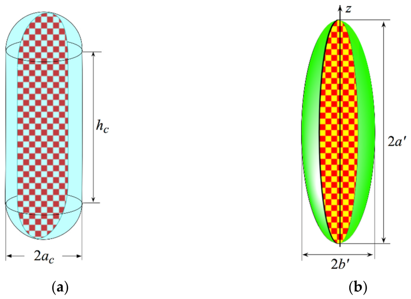
The determination of the NR representation of the voltage requires as first step to select a convex rotational surface, say Σ, shaping the long AUT as tightly as possible. For this AUT, a prolate spheroid with semi-axes a’ and b’ [25], or a cylinder of height $h_c$ ended into two hemispheres of radius $a_c$, also referred to as cigar or rounded cylinder [26] due to its shape, can be chosen, depending on the geometry of the given AUT (see Figure 2). For instance, the cigar can be conveniently adopted to model a long AUT with a constant transverse cross-section, whilst the prolate spheroid is able to best fit a long AUT with varying cross-section, through a proper choice of its semi-axes. Once the modeling surface is established, each of the meridians and parallels describing the spherical scanning surface has to be represented by an optimal parameter η. Furthermore, the expressions V of the voltage $V_p$ and $V_r$ detected by the probe and rotated probe along these curves have to be cut back by a phase factor ${\mathrm{e}}^{\mathrm{j}\psi }$, ψ being a phase function to be optimally evaluated. The so-called “reduced voltage” $\tilde{V}(\eta )=V(\eta ){\mathrm{e}}^{\mathrm{j}\psi \left(\eta \right)}$ remains defined in such a way, which, as shown in [36], is a spatially quasi-band-limited function. Accordingly, it can be reliably approximated by a strictly band-limited function as soon as its bandwidth is suitably broadened to exceed the cutoff value $W_{\eta }$ [36,37]. This is made possible by using a bandwidth excess factor ${\chi }^{\prime }$, slightly larger than the unit for AUTs of large electrical sizes [36,37].

The relations to be used for evaluating the NR representation on a meridian for the bandwidth $W_{\eta }$, the optimal parameter η and phase function ψ are:

$$W_{\eta }={\mathcal{l}}^{\prime }/\lambda$$

(1)

$$\eta =\left(\mathsf{\pi }/{\mathcal{l}}^{\prime }\right)\left[R_1+s_1^{\prime }-R_2+s_2^{\prime }\right]$$

(2)

$$\psi =\left(\mathsf{\pi }/\lambda \right)\left[R_1+s_1^{\prime }+R_2-s_2^{\prime }\right]$$

(3)

In these last equations, λ represents the wavelength and the parameter ${\mathcal{l}}^{\prime }$ denotes the length of the curve $C^{\prime }$, resulting from the intersection of Σ with the meridian plane through P. Moreover, $R_{1,2}$ and $s_{1,2}^{\prime }$ are the distances from P to the tangency points $P_{1,2}$ on curve $C^{\prime }$ and their corresponding curvilinear abscissas, respectively [10,36]. Their evaluation depends on the surface Σ adopted to model the considered long AUT [10,36]. Thus, when the best fitting of the AUT is obtained by using a cigar, the length ${\mathcal{l}}^{\prime }$ is calculated as ${\mathcal{l}}^{\prime }=2(h_c + \mathsf{\pi }{a}_c)$ and the parameter η and the phase function ψ is determined by substituting into relations (2) and (3) the appropriate values of $R_{1,2}$ and $s_{1,2}^{\prime }$ which change depending on P [26]. When utilizing the prolate spheroid to model the AUT, the length of the curve is obtained as [10,25] ${\mathcal{l}}^{\prime }=4a\prime E(\mathsf{\pi }/2\left| {\epsilon }^2\right.)$, wherein E(·|·) is the incomplete elliptic integral of the second kind, $\epsilon =f/a^{\prime }$ the spheroid eccentricity and f the hemi-focal distance. Furthermore, it has been proved [10,36] that, in any meridian plane, the curves defined by constant ψ and constant η are ellipses and hyperbolas sharing the same foci of $C^{\prime }$. These curves depend fully on the elliptical coordinates $u=(r_1-r_2)/2f$, $v=(r_1+r_2)/2f$, $r_{1,2}$ being the distances from P to the foci. As detailed in [10,25,36], these expressions are computed by using the E(·|·) function.

With regard to the NR representation on a parallel, it has been shown [10,36] that the phase function ψ is constant and identical to the phase function of the meridian passing through a given point P on that parallel and the angle φ is properly used to parameterize it. The corresponding bandwidth is defined as:

$$W_{\phi }={\displaystyle \frac{\mathsf{\pi }}{\lambda }} \underset{z^{\prime }}{\max }\left(\sqrt{{(z-z^{\prime })}^2+{(\rho +{\rho }^{\prime }(z^{\prime }))}^2}\right.\left.- \sqrt{{(z-z^{\prime })}^2+{(\rho -{\rho }^{\prime }(z^{\prime }))}^2}\right)$$

(4)

and it has been proved [36] that maximum is on the same side of the scanning parallel relative to the greatest transverse circle of Σ. In relation to Equation (4), ${\rho }^{\prime }(z^{\prime })$ is the radius of the circle of Σ at $z^{\prime }$ and $\rho =d\sin \vartheta$, $z=d\cos \vartheta$.

For the cigar, the $z^{\prime }$-value at which the sought maximum occurs is explicitly reported in [26]. In the case of the prolate spheroid, the maximum is evaluated with reference to the observation circumference tending to infinity along the curve η = constant, thus giving

$$W_{\phi }\left(\eta \right)=\beta b^{\prime }\sin {\vartheta }_{\infty }$$

(5)

wherein ${\vartheta }_{\infty }={\sin }^{-1}u+\mathsf{\pi }/2$ [25,36].

Whatever the AUT modeling choice, the resulting NF lattice is arranged as sampling parallels equispaced in the parameter η by

$$\Delta \eta =2\mathsf{\pi }/(2N^{″}+1)$$

(6)

wherein

$$N^{″}=⌊\chi N^{\prime }⌋+1;N^{\prime }=⌊{\chi }^{\prime }{W}_{\eta }⌋+1$$

(7)

χ > 1 is an oversampling factor [10,36] and $⌊·⌋$ the floor function. On each of these parallels, the NF samples are distributed at a sampling step $\Delta {\phi }_n$,

$$\Delta {\phi }_n=2 \mathsf{\pi }/(2M_n^{″}+1)$$

(8)

wherein

$$M_n^{″}=⌊\chi M_n^{\prime }⌋+1;M_n^{\prime }=⌊{\chi }^{*}{W}_{\phi }({\eta }_n)⌋+1$$

(9)

${\chi }^{*}$ being the azimuthal bandwidth excess factor [10,36]. As one can easily understand, the number of sampling points decreases on moving toward the poles.

Then, the voltage values at any point P on the measurement sphere, as well as the input NF data for the traditional spherical NtFF [16], can be accurately obtained via the 2-D OSI formula

$$V\left(\eta (\vartheta ),\phi \right) ={ \mathrm{e}}^{-\mathrm{j}\psi (\eta )} {\displaystyle {\displaystyle \sum _{n=n_0-q+1}^{n_0+q}}\left\{OF\left(\eta ,{\eta }_n,\overline{\eta },N,N^{″}\right)\right.}{\displaystyle {\displaystyle \sum _{m=m_0-p+1}^{m_0+p}} \left.\tilde{V} \left({\eta }_n,{\phi }_{m,n}\right)OF\left(\phi ,{\phi }_{m,n},\overline{\phi },M_n,M_n^{″}\right)\right\}}$$

(10)

where $n_0=⌊\eta /\Delta \eta ⌋$ and $m_0=⌊\phi /\Delta {\phi }_n⌋$ denote the indexes of the NF sample closest to P, $2q\times 2p$ the numbers of reduced voltage samples $\tilde{V} \left({\eta }_n,{\phi }_{m,n}\right)$ involved in the interpolations, and

$${\eta }_n=n\Delta \eta ;{\phi }_{m,n}=m\Delta {\phi }_n$$

(11)

$$N=N^{″}-N^{\prime };M_n=M_n^{″}-M_n^{\prime }$$

(12)

$$\overline{\eta }=q\Delta \eta ;\overline{\phi }=p\Delta {\phi }_n$$

(13)

In (10), OF denotes the interpolation function

$$OF\left(\alpha , {\alpha }_k,\overline{\alpha },L,L^{″}\right)=D_{L^{″} }\left(\alpha - {\alpha }_k\right){\mathsf{\Omega }}_{ L}\left[\left(\alpha - {\alpha }_k\right),\overline{\alpha }\right]$$

(14)

$D_{L^{″}}(·)$ and ${\mathsf{\Omega }}_{ L}(·)$ being the Dirichlet and Tschebyscheff sampling functions [10,36].

3. Correction of 3-D Probe Positioning Errors Affected NF Samples

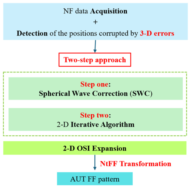
Let us suppose that, save for the sample at the north pole, the other ones do not correspond to the sampling points (6) and (8) dictated by the devised NR representation, due to the low accuracy of the AUT/probe positioners and of the controllers guiding them. Moreover, all collected NF samples also exhibit radial shifts. Accordingly, the NF collection is compromised by 3-D mispositioning errors, which will severely impair the subsequent post-processing results. In any case, the use of laser track devices can help pinpoint the exact acquisition points. According to the above hypotheses, the correction problem can be cast as two independent problems: the former related to the shifts from the set scanning radius, the latter due to the misplacements from the set NR sampling points over the nominal spherical scan surface. This enables to devise a two-step procedure (see Figure 3).

In the first step, a phase correction, named SWC to align with the wave expansion assumptions used for FF pattern evaluation, is here adopted to correct the radial shifts of the mispositioned NF samples. Let the radial deviation of the s-th sampling point from the nominal measurement sphere be denoted by ${\delta }_s$ (for $s=1,\dots ,N_T$) and $V(d+{\delta }_s, \vartheta ,\phi )$ be the corresponding voltage sample. To restore the ideal phase on the intended scan sphere, the SWC procedure compensates for this shift by multiplying the acquired voltage $V(d+{\delta }_s, \vartheta ,\phi )$ by the correction factor ${\mathrm{e}}^{\mathrm{j} 2\mathsf{\pi } {\delta }_s/\mathsf{\lambda }}$, thus giving

$$V(d,\vartheta ,\phi )={\mathrm{e}}^{\mathrm{j} 2\mathsf{\pi } {\delta }_s/\mathsf{\lambda }}V(d+{\delta }_s, \vartheta ,\phi )$$

(15)

At this point, each voltage value results to be projected onto the scan sphere, though it remains subject to a 2-D positioning error. Two well-established correction methods exist for such errors when adopting NR NF scanning: the iterative technique based and the singular value decomposition-based approaches [47,48]. The first approach requires a one-to-one mapping between the erroneous non-uniform sample and the nearest uniform sample on the NR grid. The second is applicable when the intrinsic 2-D problem can be decoupled into two 1-D problems to save computation time. Since the samples distribution resulting from the first step naturally meets the criteria for the iterative technique based method, this last approach is utilized to restore the NF samples at the correct NR grid points.

According to such considerations, the reduced voltage at any non-uniform sampling point $({\varsigma }_k,{\sigma }_{j,k})$ can be expressed in terms of the unknown reduced voltage values at the nearest uniform ones $\left({\eta }_n,{\phi }_{m,n}\right)$ through the OSI formula (10), thus obtaining:

$$\tilde{V}({\varsigma }_k,{\sigma }_{j,k})={\displaystyle {\displaystyle \sum _{n=n_0-q+1}^{n_0+q}}\left\{OF\left({\varsigma }_k,{\eta }_n, \overline{\eta },N,N^{″}\right)\right.}{\displaystyle {\displaystyle \sum _{m=m_0-p+1}^{m_0+p}}\left.\tilde{V} \left({\eta }_n,{\phi }_{m,n}\right)OF\left({\sigma }_{j,k},{\phi }_{m,n},\overline{\phi }, M_n,M_n^{″}\right)\right\}}$$

(16)

Expressing relation (16) in matrix form yields

$$\underset{¯}{\underset{¯}{\Lambda }} \underset{\_}{U}=\underset{¯}{NU}$$

(17)

wherein $\underset{\_}{U}$ is the column vector of the unknown uniform samples $\tilde{V} \left({\eta }_n,{\phi }_{m,n}\right)$, $\underset{¯}{\underset{¯}{\Lambda }}$ is a $N_T\times N_T$-sized banded matrix, whose elements are given by the interpolation functions, and $\underset{¯}{NU}$ the column vector of the known non-uniform samples $\tilde{V}({\varsigma }_k,{\sigma }_{j,k})$. The 3-D errors correction process is then completed by solving this linear system. To this end, the aforementioned iterative technique is adopted [48]. Firstly, relation (17) is rearranged by subdividing $\underset{¯}{\underset{¯}{\Lambda }}$ into its diagonal ${\underset{¯}{\underset{¯}{\Lambda }}}_D$ and non-diagonal $\underset{¯}{\underset{¯}{\Gamma }}$ parts, then both its terms are multiplied by ${\underset{¯}{\underset{¯}{\Lambda }}}_D^{ -1}$, leading to the following expression:

$${\underset{¯}{U}}^{(\nu )} ={\underset{¯}{U}}^{(0)}- {\underset{¯}{\underset{¯}{\Lambda }}}_D^{ -1}\underset{¯}{\underset{¯}{\Gamma }} {\underset{¯}{U}}^{(\nu -1)}$$

(18)

where ${\underset{¯}{U}}^{(\nu )}$ is the vector of the samples restored at the ν-th iteration and ${\underset{¯}{U}}^{(0)} = {\underset{¯}{\underset{¯}{\Lambda }}}_D^{ -1}\underset{¯}{NU}$. By rewriting relation (18) in explicit form, it results in

$$\begin{gathered} {\tilde{V}}^{(\nu )}\left({\eta }_n,{\phi }_{m,n}\right)={\displaystyle \frac{1}{OF\left({\varsigma }_n,{\eta }_n,\overline{\eta } ,N,N^{″}\right)OF({\sigma }_{m,n},{\phi }_{m,n},{\overline{\phi }}_n, M_n,M_n^{″})}} \\ \begin{array}{ll}\cdot \{\tilde{V}\left({\varsigma }_n,{\sigma }_{m,n}\right)-& {\displaystyle \sum _{k=k_0-q+1}^{k_0+q}}{\displaystyle \sum _{j=j_0-p+1}^{j_0+p}OF\left({\varsigma }_n,{\eta }_k,\overline{\eta },N,N^{″}\right)}{\tilde{V}}^{(\nu -1)}\left({\eta }_k,{\phi }_{j,k}\right)\mathit{OF}\left({\sigma }_{m,n},{\phi }_{j,k},\overline{\phi },M_k,M_k^{″}\right)\}\\ & (k\ne n) \wedge (j\ne m)\end{array} \end{gathered}$$

(19)

wherein

$$j_0=\left\{\begin{array}{c}m\hspace{1em} \mathrm{if} {\sigma }_{m,n}\ge {\phi }_{m,n}\\ m-1 \mathrm{if} {\sigma }_{m,n}<{\phi }_{m,n}\end{array}\right.,\hspace{1em}{k}_0=\left\{\begin{array}{c}n \hspace{1em} \mathrm{if} {\varsigma }_n\ge {\eta }_n\\ n-1 \mathrm{if} {\varsigma }_n< {\eta }_n\end{array}\right.$$

(20)

The convergence of this iterative algorithm is usually guaranteed if $\forall i$, $i=1,\dots ,N_T$, ${\Lambda }_{ii}\ne 0$ and $\forall r\ne i$ $\left|{\Lambda }_{ii}\right|>\left|{\Lambda }_{ir}\right|$ and $\left|{\Lambda }_{ii}\right|>\left|{\Lambda }_{ri}\right|$ [48]. The abovementioned hypotheses on the 2-D samples arrangement assure that these criteria are satisfied.

4. Numerical Tests

Some numerical results assessing the accuracy of the devised two-step procedure for correcting the 3-D position errors, impairing the characterization of long AUTs in a SNF facility, are shown in this section.

Two different AUTs, both operating at 10 GHz, are considered in the reported simulation results. The former is a uniform planar array of z-polarized Huygens sources in the xz-plane, covering a rectangle $14.4\mathsf{\lambda }\times 31.6\mathsf{\lambda }$-sized which ends in two semi-circles of a 7.2 λ radius. The elements are spaced by 0.6 λ in the rectangle and by 1.2 λ in the semi-circles. The latter is still a planar array of z-polarized Huygens sources, whose elements are now contained in an ellipse in the xz-plane with semi-axes equal to 21 λ and 6 λ. The elements along the x direction are spaced by 0.6 λ and uniformly excited, whilst those along z are 0.9 λ-spaced and non-uniformly excited with a triangular amplitude tapering.

The former AUT (CASE1) exhibits a constant transverse cross-section and, accordingly, has been modeled by a cigar having $h_c$ = 31.6 λ and $a_c$ = 7.2 λ; the latter (CASE2), showing a varying cross-section, has been modeled by a prolate spheroid with semi-axes a’ and b’ equal to 21 λ and 6 λ, respectively.

The shown results are relevant to NF measurements collected by an X-band open-ended rectangular waveguide over scanning spheres of radii d = 32 λ and 30 λ for CASE1 and CASE2, respectively. Moreover, to deal with NF data corrupted by 3-D probe positioning errors, each radial coordinate of the simulated NF samples is shifted with respect to the set radius d by a deviation ${\delta }_s$, modeled as a random variable uniformly distributed in the range [−0.1 λ, 0.1 λ]. Also their η and φ values have been shifted with respect to those corresponding to the utilized NR sampling arrangement. The shifts have been again modeled as random variables, but now they are uniformly distributed in the ranges of $[-\Delta \eta /3,\Delta \eta /3]$ and $[-\Delta {\phi }_n/3,\Delta {\phi }_n/3]$, respectively.

In order to appraise the effectiveness of the two-step procedure, the amplitude and phase reconstructions of the voltage obtained from the positioning errors affected NF data are compared in the following to the corresponding exact patterns and to those attained by directly interpolating the misplaced samples. Furthermore, results relevant to the behavior of the compensation procedure when using only one of the two proposed steps are also shown.

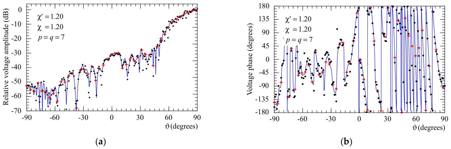
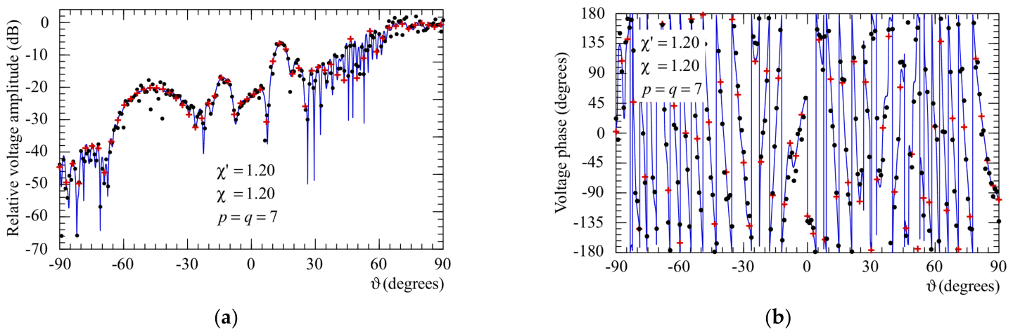
Figure 4 is relevant to CASE1, whilst Figure 5 refers to CASE2, both corresponding to the cut plane at φ = 90°.

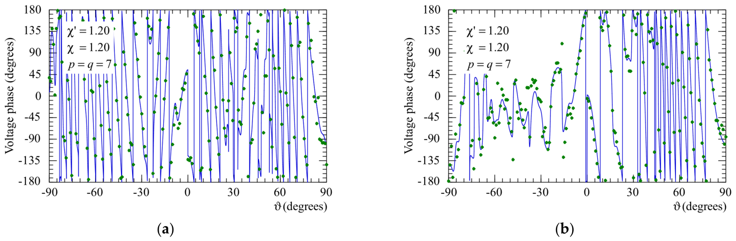
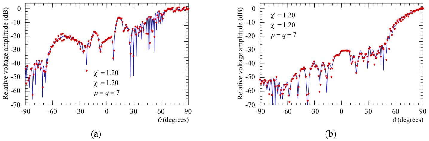
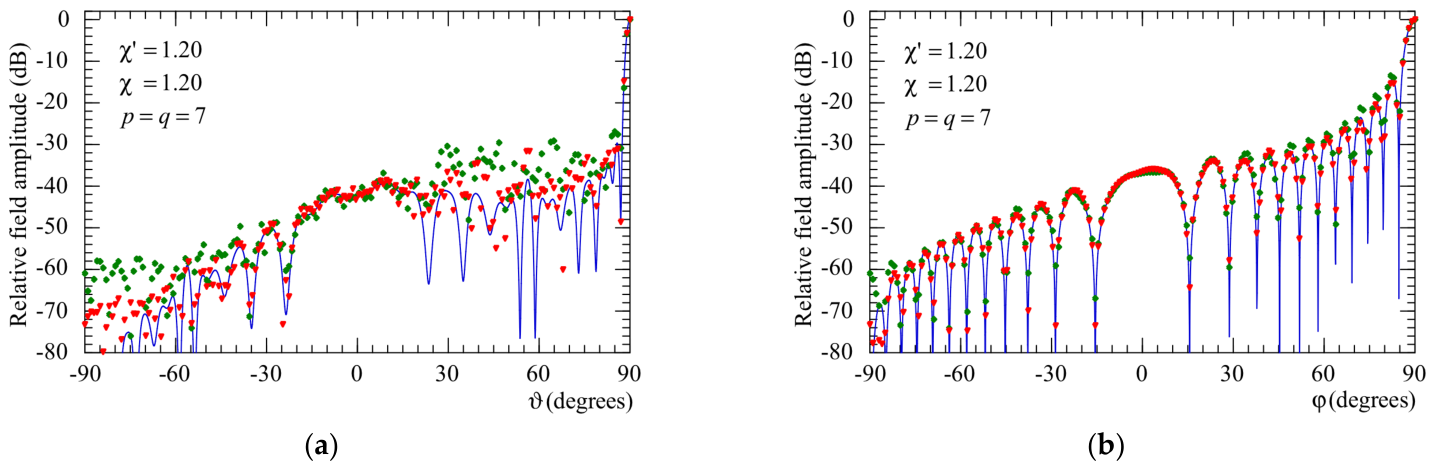
As can be seen, in both cases, the NF reconstructions obtained by using the devised two-step technique are very accurate even when the NF samples are impaired by severe 3-D positioning errors. On the other hand, those obtained without applying such a technique are strongly deteriorated. Moreover, the recoveries of voltage phase when using only the iterative algorithm (19) (Figure 6) and those of the voltage amplitude when applying only the SWC approach (15) (Figure 7) show that both steps have to be performed to improve the accuracy of the reconstructions and to prevent a significant degradation of the precision.

As shown in [47,48], the iterative algorithm entails very short times and, in the reported examples, only 10 iterations have been sufficient for its convergence.

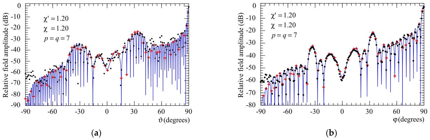
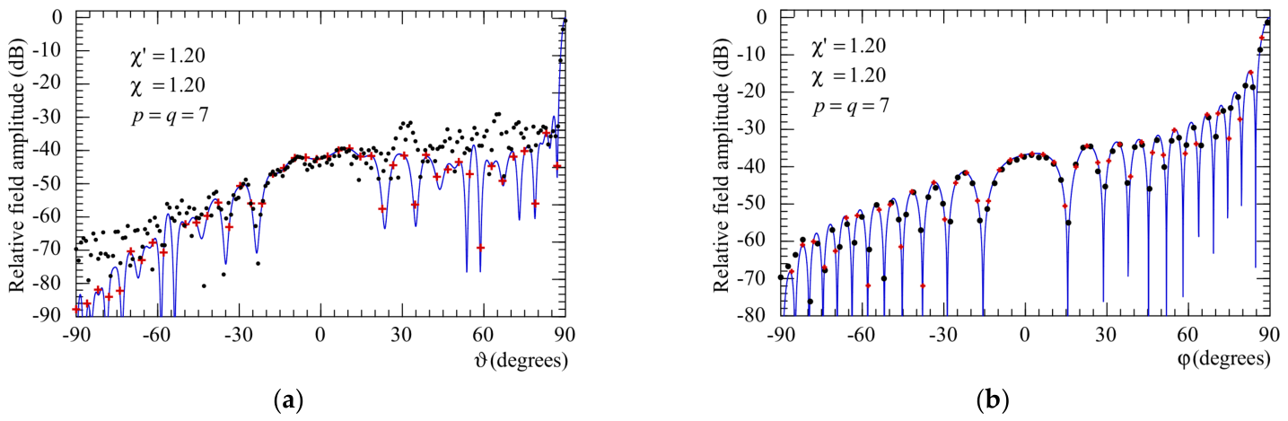
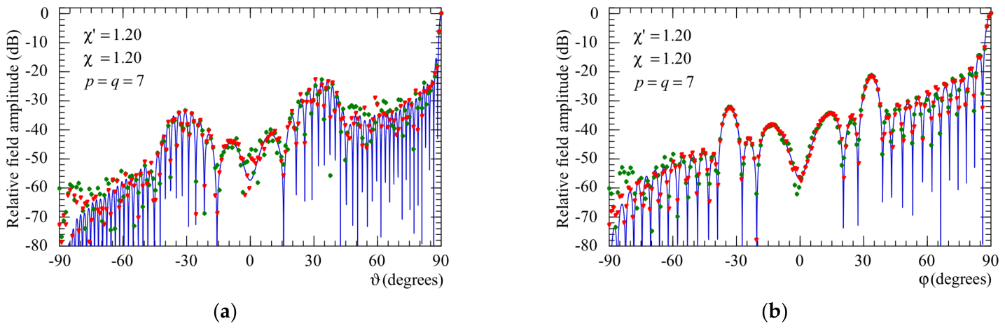
It is worth emphasizing that the NR sampling scheme requires the acquisition of only 18,693 NF samples for CASE1 and 11,606 for CASE2. The overall accuracy of the two-step compensation procedure has been tested by applying it to the NR samples and then interpolating, via (10), both the corrupted and the error-compensated datasets to retrieve the much larger number of input samples required for the classical NtFF transformation [16], namely, 51,520 samples for CASE1 and 41,760 for CASE2. The resulting E- and H-plane FF patterns have been then compared to the exact ones in Figure 8 (CASE1) and Figure 9 (CASE2). As can be easily noted, the FF reconstructions achieved by using the developed approach are accurate everywhere as compared to those that do not use it. Moreover, the FF results confirm the behavior observed for the NF ones (see Figure 10 and Figure 11), which highlighted the need to follow the SWC phase correction with the iterative algorithm to attain high precision and a reliable reconstruction of the antenna far field.

It can be interesting to provide a quantitative insight of the accuracy of the devised two-step technique by comparing the mean-square error achieved in the E-plane pattern reconstructions to those resulting without applying it. In particular, the mean-square error is −68.61 dB for CASE1 and −68.93 dB for CASE2 when applying the developed procedure and is −39.84 dB for CASE1 and −39.05 dB for CASE2 without using it. These values must be compared to those obtained when using only SWC (−45.57 dB for CASE1 and −47.80 dB for CASE2) or the iterative algorithm (−44.99 dB for CASE1 and −41.44 dB for CASE2), thus further confirming the need of using both steps.

5. Conclusions

This paper presents a feasibility study, performed through an extensive and accurate numerical validation, on the compensation of 3-D probe position errors, which can occur in the characterization of long AUTs in a SNF facility, at the points of the sampling arrangement devised by adopting one of the two available modeling types (prolate spheroid or cigar). The proposed solution is a two-step procedure: first, a SWC phase correction addresses radial shifts from the scan sphere; second, an iterative technique resolves the remaining 2-D positioning errors. Numerical simulations on two different AUTs prove the effectiveness of this approach and confirm that both steps are necessary for accurate NF and FF reconstructions. Future experimental validation will be conducted at partner laboratories, followed by testing at the University of Salerno’s NF facility once the needed upgrades are completed.

References

1. Yaghjian, A.D. An overview of near-field antenna measurements. IEEE Trans. Antennas Propag. 1986, 34, 30–45. [Google Scholar] [CrossRef]
2. Appel-Hansen, J.; Dyson, J.D.; Gillespie, E.S.; Hickman, T.G. Antenna Measurements. In The Handbook of Antenna Design; Rudge, A.W., Milne, K., Olver, A.D., Knight, P., Eds.; Peter Peregrinus: London, UK, 1986; pp. 584–694. [Google Scholar]
3. Gillespie, E.S. Special Issue on near-field scanning techniques. IEEE Trans. Antennas Propag. 1988, 36, 727–901. [Google Scholar]
4. Slater, D. Near-Field Antenna Measurements; Artech House: Boston, MA, USA, 1991. [Google Scholar]
5. Gregson, S.F.; McCormick, J.; Parini, C.G. Principles of Planar Near-Field Antenna Measurements; IET: London, UK, 2007. [Google Scholar]
6. Francis, M.H.; Wittmann, R.C. Near-Field Scanning Measurements: Theory and Practice. In Modern Antenna Handbook; Balanis, C.A., Ed.; John Wiley & Sons Inc.: Hoboken, NJ, USA, 2008; pp. 929–976. [Google Scholar]
7. IEEE Standard 1720-2012; IEEE Recommended Practice for Near-Field Antenna Measurements. Francis, M.H., Ed.; IEEE: New York, NY, USA, 2012.
8. Sierra Castañer, M.; Foged, L.J. Post-Processing Techniques in Antenna Measurement; SciTech Publishing IET: London, UK, 2019. [Google Scholar]
9. Parini, C.; Gregson, S.; McCormick, J.; Van Resburg, D.J.; Eibert, T. Theory and Practice of Modern Antenna Range Measurements; SciTech Publishing IET: London, UK, 2020. [Google Scholar]
10. Ferrara, F.; Gennarelli, C.; Guerriero, R.; D’Agostino, F. Non-Redundant Near-Field to Far-Field Transformation Techniques; SciTech Publishing IET: London, UK, 2022. [Google Scholar]
11. Jensen, F. On the probe compensation for near-field measurements on a sphere. Arch. Elektr. Übertr. 1975, 29, 306–308. [Google Scholar]
12. Wacker, P.F. Non-Planar Near-Field Measurements: Spherical Scanning; NBSIR 75-809; National Institute of Standards and Technology: Boulder, CO, USA, 1975.
13. Larsen, F.H. Probe correction of spherical near-field measurements. Electr. Lett. 1977, 13, 393–395. [Google Scholar] [CrossRef]
14. Yaghjian, A.D.; Wittmann, R.C. The receiving antenna as a linear differential operator: Application to spherical near-field measurement. IEEE Trans. Antennas Propag. 1985, 33, 1175–1185. [Google Scholar]
15. Hansen, J.E.; Jensen, F. Spherical near-field scanning at the technical university of Denmark. IEEE Trans. Antennas Propag. 1988, 36, 734–739. [Google Scholar]
16. Hald, J.; Hansen, J.E.; Jensen, F.; Larsen, F.H. Spherical Near-Field Antenna Measurements; Hansen, J.E., Ed.; Peregrinus: London, UK, 1998. [Google Scholar]
17. Laitinen, T.; Pivnenko, S. Probe correction technique for symmetric odd-order probes for spherical near-field antenna measurements. IEEE Antennas Wirel. Propag. Lett. 2007, 6, 635–638. [Google Scholar]
18. Las-Heras, F.; Sarkar, T.K. Radial field retrieval in spherical scanning for current reconstruction and NF–FF transformation. IEEE Trans. Antennas Propag. 2002, 50, 866–874. [Google Scholar]
19. Laitinen, T. Double φ-step θ-scanning technique for spherical near-field antenna measurements. IEEE Trans. Antennas Propag. 2008, 56, 1633–1639. [Google Scholar]
20. Laitinen, T. Modified θ-scanning technique for first/third-order probes for spherical near-field antenna measurements. IEEE Trans. Antennas Propag. 2008, 57, 1590–1596. [Google Scholar]
21. Alvarez, Y.; Las-Heras, F.; Pino, M.R. On the comparison between the spherical wave expansion and the sources reconstruction method. IEEE Trans. Antennas Propag. 2008, 56, 3337–3341. [Google Scholar] [CrossRef]
22. Laitinen, T.; Pivnenko, S.; Nielsen, J.M.; Breinbjerg, O. Theory and practice of the FFT/matrix inversion technique for probe-corrected spherical near-field antenna measurements with high-order probes. IEEE Trans. Antennas Propag. 2010, 58, 2623–2631. [Google Scholar]
23. Hansen, T.B. Spherical near-field scanning with higher-order probes. IEEE Trans. Antennas Propag. 2011, 59, 4049–4059. [Google Scholar]
24. Hansen, T.B. Numerical investigation of the system-matrix method for higher-order probe correction in spherical near-field antenna measurements. Int. J. Antennas Propag. 2012, 2012, 493705. [Google Scholar]
25. D’Agostino, F.; Ferrara, F.; Gennarelli, C.; Guerriero, R.; Migliozzi, M. Non-redundant spherical NF—FF transformations using ellipsoidal antenna modeling: Experimental assessments. IEEE Antennas Propag. Mag. 2013, 55, 166–175. [Google Scholar]
26. D’Agostino, F.; Ferrara, F.; Gennarelli, C.; Guerriero, R.; Migliozzi, M. Experimental testing of nonredundant near-field to far-field transformations with spherical scanning using flexible modelings for nonvolumetric antennas. Int. J. Antennas Propag. 2013, 2013, 517934. [Google Scholar]
27. Qureshi, M.A.; Schmidt, C.H.; Eibert, T.F. Adaptive sampling in spherical and cylindrical near-field antenna measurements. IEEE Antennas Propag. Mag. 2013, 55, 243–249. [Google Scholar] [CrossRef]
28. Cornelius, R.; Heberling, D. Spherical near-field scanning with pointwise probe correction. IEEE Trans. Antennas Propag. 2017, 65, 995–996. [Google Scholar]
29. Varela, F.R.; Iragüen, B.G.; Sierra Castañer, M. Under-sampled spherical near-field antenna measurements with error estimation. IEEE Trans. Antennas Propag. 2020, 68, 6364–6371. [Google Scholar]
30. Cornelius, R.; Heberling, D.; Koep, N.; Behboodi, A.; Mathar, R. Compressed sensing applied to spherical near-field to far-field transformation. In Proceedings of the European Conference on Antennas and Propagation, Davos, Switzerland, 10–15 April 2016; pp. 1–4. [Google Scholar]
31. Culotta-López, C.; Heberling, D.; Bangun, A.; Behboodi, A.; Mathar, R. A compressed sampling for spherical near-field measurements. In Proceedings of the Antenna Measurement Techniques Association (AMTA) Symposium, Williamsburg, VA, USA, 4–9 November 2018; pp. 1–6. [Google Scholar]
32. Bangun, A.; Culotta-López, C. Optimizing sensing matrices for spherical near-field antenna measurements. IEEE Trans. Antennas Propag. 2023, 71, 1716–1724. [Google Scholar]
33. Peng, F.; Zhang, Q.; Liu, X.; Wang, Z.; Chen, X. An efficient antenna measurements method in spherical near field based on sparse sampling. IEEE Antennas Wirel. Propag. Lett. 2024, 23, 3492–3496. [Google Scholar] [CrossRef]
34. Park, S.-H.; Jang, G.-H.; Seo, Y.-H.; Keum, H.-S.; Bang, S.-I. High-speed antenna measurement system using multi-probe array technique for 5G applications. Electronics 2022, 11, 3435. [Google Scholar]
35. Zhang, R.; Zhang, S.; Wang, Z.; Song, Z.; Bai, C. A novel analytical method for eliminating the multiprobe array and environment interference in spherical near-field measurement. IEEE Trans. Instrum. Meas. 2025, 74, 6002714. [Google Scholar] [CrossRef]
36. Bucci, O.M.; Gennarelli, C.; Savarese, C. Representation of electromagnetic fields over arbitrary surfaces by a finite and nonredundant number of samples. IEEE Trans. Antennas Propag. 1998, 46, 351–359. [Google Scholar] [CrossRef]
37. Bucci, O.M.; Franceschetti, G. On the spatial bandwidth of scattered fields. IEEE Trans. Antennas Propag. 1987, 35, 1445–1455. [Google Scholar] [CrossRef]
38. Bucci, O.M.; Franceschetti, G. On the degrees of freedom of scattered fields. IEEE Trans. Antennas Propag. 1989, 37, 918–926. [Google Scholar] [CrossRef]
39. Bucci, O.M.; Migliore, M.D. Degrees of freedom and sampling representation of electromagnetic fields: Concepts and applications. IEEE Trans. Antennas Propag. 2025, 67, 10–22. [Google Scholar]
40. Wittmann, R.C.; Alpert, B.K.; Francis, M.H. Near-field antenna measurements using nonideal measurement locations. IEEE Trans. Antennas Propag. 1998, 46, 716–722. [Google Scholar] [CrossRef]
41. Farouq, M.; Serhir, M.; Picard, D. Matrix method for far-field calculation using irregular near-field samples for cylindrical and spherical scanning surfaces. Prog. Electromagn. Res. 2015, 63, 35–48. [Google Scholar]
42. Wittmann, R.C.; Alpert, B.K.; Francis, M.H. Near-field, spherical scanning antenna measurements with nonideal probe locations. IEEE Trans. Antennas Propag. 2004, 52, 2184–2186. [Google Scholar] [CrossRef]
43. Bevilacqua, F.; D’Agostino, F.; Ferrara, F.; Gennarelli, C.; Guerriero, R.; Migliozzi, M.; Riccio, G. Pattern reconstruction from near-field data affected by 3D probe positioning errors collected via planar-wide mesh scanning. Electronics 2023, 12, 542. [Google Scholar]
44. D’Agostino, F.; Ferrara, F.; Gennarelli, C.; Guerriero, R.; Migliozzi, M.; Pascarella, L.; Riccio, G. Three- dimensional probe mispositioning errors compensation: A feasibility study in the non-redundant helicoidal near to far-field transformation case. Electronics 2024, 13, 3767. [Google Scholar]
45. D’Agostino, F.; Ferrara, F.; Gennarelli, C.; Guerriero, R.; Migliozzi, M.; Pascarella, L. An effective two-step procedure allowing the retrieval of the non-redundant spherical near-field samples from the 3-D mispositioned ones. Sensors 2025, 25, 5626. [Google Scholar] [PubMed]
46. Joy, E.B.; Wilson, R.E. A simplified technique for probe position error compensation in planar surface near-field measurements. In Proceedings of the 1982 Antenna Measurement Techniques Association (AMTA) Symposium, Las Cruces, NM, USA, 5–7 October 1982; pp. 14.1–14.10. [Google Scholar]
47. D’Agostino, F.; Ferrara, F.; Gennarelli, C.; Guerriero, R.; Migliozzi, M. On the compensation of probe positioning errors when using a nonredundant cylindrical NF–FF transformation. Prog. Electromagn. Res. B. 2010, 20, 321–335. [Google Scholar]
48. D’Agostino, F.; Ferrara, F.; Gennarelli, C.; Guerriero, R.; Migliozzi, M. Probe position errors corrected near-field-far-field transformation with spherical scanning. Appl. Comp. Electromagn. Soc. J. 2016, 31, 106–117. [Google Scholar]
49. Bucci, O.M.; D’Elia, G.; Migliore, M.D. Advanced field interpolation from plane-polar samples: Experimental verification. IEEE Trans. Antennas Propag. 1998, 46, 204–210. [Google Scholar]
Figure 1. SNF scanning.
Electronics 15 02961 g001
Figure 2. (a) Cigar. (b) Prolate spheroid.
Electronics 15 02961 g002
Figure 3. Flowchart of the two-step method.
Electronics 15 02961 g003
Figure 4. Amplitude (a) and phase (b) of V r on the meridian at φ = 90° (CASE 1). ––––– exact. + + + + obtained from the misplaced NF samples using the devised method.                   obtained without its use.
Electronics 15 02961 g004
Figure 5. Amplitude (a) and phase (b) of V r on the meridian at φ = 90° (CASE2). ––––– exact. + + + + obtained from the misplaced NF samples using the devised method.                   obtained without its use.
Electronics 15 02961 g005
Figure 6. Phase of V r on the meridian at φ = 90°. ––––– exact. ◆◆◆◆ got from the misplaced NF samples using only the iterative technique. (a) CASE1; (b) CASE2.
Electronics 15 02961 g006
Figure 7. Amplitude of V r on the meridian at φ = 90°. ––––– exact. ▼▼▼▼ obtained from the misplaced NF samples using only the SWC. (a) CASE1; (b) CASE2.
Electronics 15 02961 g007
Figure 8. FF patterns (CASE1). E-plane (a) H-plane (b). ––––– exact. + + + + obtained from the misplaced NF samples using the devised method.                   obtained without its use.
Electronics 15 02961 g008
Figure 9. FF patterns (CASE2). E-plane (a) H-plane (b) ––––– exact. + + + + obtained from the misplaced NF samples using the devised method.                   obtained without its use.
Electronics 15 02961 g009
Figure 10. FF patterns (CASE1). E-plane (a) H-plane (b) ––––– exact.▼▼▼▼obtained from the misplaced NF samples using only the SWC. ◆◆◆◆ obtained from the misplaced NF samples using only the iterative technique.
Electronics 15 02961 g010
Figure 11. FF patterns (CASE2). E-plane (a) H-plane (b) ––––– exact.▼▼▼▼obtained from the misplaced NF samples using only the SWC. ◆◆◆◆ obtained from the misplaced NF samples using only the iterative technique.
Electronics 15 02961 g011
Disclaimer/Publisher’s Note: The statements, opinions and data contained in all publications are solely those of the individual author(s) and contributor(s) and not of MDPI and/or the editor(s). MDPI and/or the editor(s) disclaim responsibility for any injury to people or property resulting from any ideas, methods, instructions or products referred to in the content.