Fault-Tolerant Constrained Control of Nonlinear Active Suspension Systems Using Adaptive Filtering and Neural Approximation

Abstract

This paper investigates the fault-tolerant constrained control problem of a nonlinear quarter-car active suspension system subject to road disturbances, body-state constraints, and mixed actuator faults. When mixed actuator faults, state constraints, unknown nonlinear suspension dynamics, and convergence-time requirements coexist, it remains challenging to simultaneously guarantee fault-tolerant compensation, constraint preservation, and implementable control laws. To address these challenges, a neural-network control method based on an adaptive prescribed-time filter (APF) is proposed. A logarithmic state transformation is introduced to convert the body-displacement and velocity constraints into boundedness problems of transformed variables, and the sprung-mass subsystem is represented in a strict-feedback form. The unknown nonlinearities induced by suspension dynamics, road disturbances, and additive actuator faults are approximated online by radial basis function neural networks. Meanwhile, the APF is employed to avoid repeated differentiation of virtual control laws in backstepping and to achieve practical prescribed-time stability. Lyapunov analysis proves that all closed-loop signals are bounded, the body-state constraints are preserved, and sufficient conditions are obtained for the boundedness of the unsprung-mass dynamics, as well as the safety of suspension travel and tire dynamic load. Simulation results under sinusoidal road excitation and smooth-transition actuator faults show that, compared with PID control, passive suspension, and sliding mode control, the proposed method reduces the body-displacement RMSE by 77.39%, 91.83%, and 73.12%, respectively, and the RMS body acceleration by 70.34%, 87.73%, and 50.22%, respectively, while maintaining suspension travel and tire dynamic load within their safety bounds.

1. Introduction

With increasing vehicle speeds and growing requirements for ride comfort and driving safety, active suspension systems have become an important chassis technology for improving vehicle vertical dynamics. Compared with passive suspensions, active suspensions introduce an actuator force between the vehicle body and the wheel, which enables active regulation of the suspension force and improves vibration suppression under road disturbances. Hrovat presented a systematic survey of advanced suspension developments and related optimal control applications, showing that quarter-car, half-car, and full-car models can all be used for active suspension controller design [1]. Subsequently, various advanced control methods, such as $H_{\infty }$ control, sampled-data control, finite-frequency control, and linear parameter-varying gain-scheduling control, have been developed to improve robustness and ride comfort under uncertain road excitations [2,3,4,5]. However, active suspension control is not a single-objective vibration suppression problem. Body displacement, body acceleration, suspension travel, tire dynamic load, and actuator output are naturally coupled, and improving one performance index may deteriorate another. Therefore, an effective active suspension controller should improve ride comfort while maintaining safety-related constraints. Recent studies have also addressed motion planning and sensor fault diagnosis for intelligent vehicles under safety-critical conditions [6,7], further highlighting the need for reliable vehicle control. In addition to vertical vibration suppression, the optimization of lateral and yaw dynamics is also important for overall vehicle stability. For example, vehicle stability regions have been estimated and expanded using region-of-attraction analysis and sums-of-squares programming [8]. Nevertheless, this paper focuses on vertical active suspension dynamics, which directly affect ride comfort, suspension travel, and tire road holding.

For vertical active suspension dynamics, existing control methods can be roughly classified into classical feedback control, robust control, sliding mode control, adaptive control, and intelligent control. Classical feedback controllers, such as PID-type methods, have simple structures and convenient implementation, but their performance strongly depends on parameter tuning. Robust control improves disturbance attenuation, whereas it may become conservative when multiple safety constraints are imposed. Sliding mode control is also widely used because of its robustness against model uncertainties and external disturbances [9,10]; however, conventional sliding mode methods may introduce chattering, and additional design efforts are required when smooth control input, fault tolerance, and state constraints are considered simultaneously.

Recent advanced feedback controllers, including adaptive PID-type, intelligent PID, fractional-order PID, BELBIC-based PID, neuroendocrine-inspired PID, and nonlinear-function-shaped PID schemes, have been developed to improve transient response, robustness, and implementation flexibility in mechatronic and vibration-control systems [11,12,13,14,15,16,17,18]. Although these methods have demonstrated good engineering performance in diverse applications, they are generally developed from the viewpoints of gain tuning, nonlinear error shaping, or intelligent parameter adjustment, rather than being primarily designed to provide a unified Lyapunov-based stability guarantee for unknown nonlinear suspension dynamics, mixed actuator-fault compensation, state-constraint preservation, and prescribed-time boundedness. This motivates the adaptive prescribed-time-filter-based neural-network backstepping framework developed in this paper.

For nonlinear active suspension systems, adaptive control and backstepping control provide a systematic framework for handling parameter uncertainties and nonlinear dynamics. Sun et al. proposed a constrained adaptive backstepping control method for uncertain nonlinear active suspension systems, in which ride comfort, suspension travel, and tire dynamic load requirements were incorporated into a unified multi-objective control framework [19]. Pang et al. investigated adaptive backstepping tracking control and coordinated adaptive backstepping control for nonlinear uncertain active suspension systems with safety constraints [20,21]. More recently, adaptive bioinspired preview suspension control with constrained velocity planning has been studied for autonomous vehicles [22]. These studies demonstrate the effectiveness of backstepping-based methods in dealing with nonlinear suspension dynamics. However, conventional backstepping usually requires the analytical differentiation of virtual control laws. As the system order increases or the virtual control law becomes complicated, this procedure may lead to the well-known “explosion of complexity” problem.

Active suspension systems commonly exhibit strong nonlinearities and uncertainties. For example, the suspension spring may have nonlinear stiffness, the damping force may be piecewise in the rebound and compression strokes, and the road input and its derivative may enter the tire dynamics. In addition, actuator faults may further increase the uncertainty of the controlled system. Neural-network-based adaptive control is an effective approach for such uncertain nonlinear systems because neural networks can approximate unknown continuous nonlinear functions on compact sets. Early studies on nonlinear adaptive active suspensions showed that parameter adaptive control combined with Lyapunov analysis can mitigate the influence of model uncertainties on control performance [23]. Radial basis function neural networks have a simple structure, clear approximation mechanism, and convenient online implementation, and have therefore been widely used to approximate unknown nonlinearities, external disturbances, and fault-related terms [24,25,26].

State constraints and actuator faults are two important issues in active suspension control. Excessive body displacement and velocity may degrade ride comfort, excessive suspension travel may lead to mechanical stop impacts, and excessive tire dynamic load may weaken tire road holding. Barrier Lyapunov functions have been widely used in nonlinear systems with output constraints and body-state constraints [27,28]. However, within the backstepping framework, BLF-based methods may introduce feasibility conditions related to constraint boundaries. As an alternative, state-transformation methods map constrained states into unconstrained variables and guarantee constraint preservation by proving the boundedness of the transformed variables [29,30]. Moreover, active suspension actuators may suffer from efficiency loss, additive bias forces, or mixed faults. Existing fault-tolerant active suspension studies have considered the influence of actuator faults on ride comfort, road holding, and suspension travel constraints [31,32,33], while finite-time fault-tolerant control with prescribed performance has also been investigated for autonomous vehicle systems [34]. Nevertheless, when mixed actuator faults, state constraints, unknown nonlinear suspension dynamics, and convergence-time requirements coexist, it remains challenging to design a controller that can simultaneously guarantee fault-tolerant compensation, constraint preservation, and implementable control laws.

To reduce the complexity of backstepping design, command-filtered control and dynamic-surface control have been introduced to avoid repeated analytical differentiation of virtual control laws [35,36]. Meanwhile, finite-time, fixed-time, and prescribed-time control methods have attracted increasing attention because they provide different forms of convergence-time guarantees. In particular, prescribed-time control allows the convergence time to be specified in advance by the designer and to be independent of the initial conditions. In recent years, prescribed-time command-filtered control, prespecified-time reliable suspension control, and adaptive prescribed-time-filtered control have been applied to uncertain nonlinear systems and vehicle suspension systems to improve convergence-time adjustability, reliability, and control-law implementability [37,38,39]. Therefore, introducing an adaptive prescribed-time filter into fault-tolerant constrained active suspension control is helpful for simultaneously addressing state-constraint preservation, unknown nonlinear approximation, actuator fault compensation, and backstepping complexity.

Motivated by the above discussion, this paper develops an adaptive prescribed-time-filter-based neural-network control method for nonlinear active suspension systems subject to mixed actuator faults, unknown nonlinearities, road disturbances, and body-state constraints. The main contributions are summarized as follows.

(1)

A unified fault-tolerant constrained control framework is developed for a nonlinear quarter-car active suspension system, where mixed actuator faults, road disturbances, and safety-related body-state constraints are explicitly considered.

(2)

A logarithmic state transformation and an adaptive prescribed-time filter are incorporated into the backstepping design. The former ensures the preservation of body-displacement and velocity constraints, while the latter avoids the analytical differentiation of the virtual control law and improves controller implementability.

(3)

An RBFNN is employed to approximate the lumped unknown nonlinearities, and Lyapunov analysis establishes practical prescribed-time boundedness and constraint preservation. The boundedness of the internal unsprung-mass dynamics and the safety requirements for suspension travel and tire dynamic load are further investigated, and comparative simulations verify the effectiveness of the proposed method.

2. System Modeling and Problem Formulation

2.1. Quarter-Car Active Suspension Dynamics

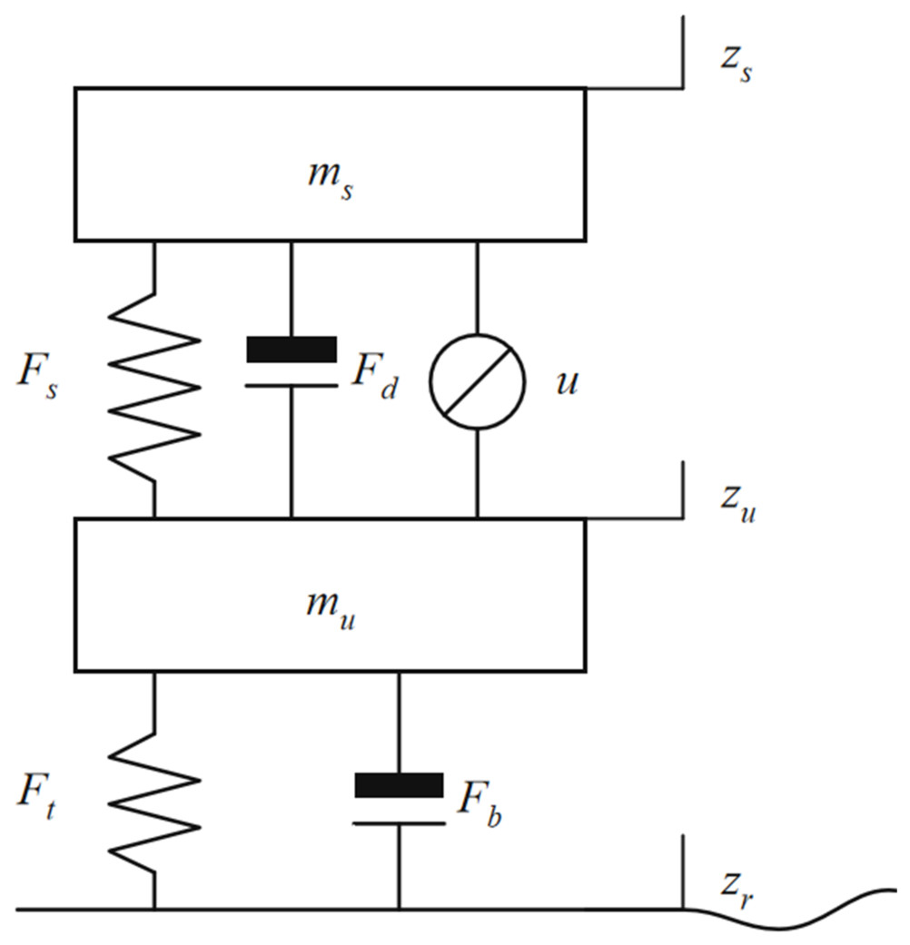
Consider the quarter-car active suspension model shown in Figure 1. This model has been widely used in active suspension control studies [19,40,41].

Let $z_s$ and $z_u$ denote the vertical displacements of the sprung and unsprung masses, respectively, $z_r$ denote the road vertical input, and $m_s$ and $m_u$ denote the corresponding masses. The system dynamics are given by

$$\begin{array}{cc}\hfill m_s{\ddot{z}}_s& =-F_d({\dot{z}}_s,{\dot{z}}_u,t)-F_s(z_s,z_u,t)+u_f\left(t\right),\hfill \\ \hfill m_u{\ddot{z}}_u& =F_d({\dot{z}}_s,{\dot{z}}_u,t)+F_s(z_s,z_u,t)\hfill \\ \hfill & -F_t(z_u,z_r,t)-F_b({\dot{z}}_u,{\dot{z}}_r,t)-u_f\left(t\right)\hfill \end{array}$$

(1)

where $u_f\left(t\right)$ is the actual output force applied by the actuator to the suspension system. The force terms represent the nonlinear spring force $F_s$, the piecewise linear damping force $F_d$, the equivalent tire elastic force $F_t$, and the equivalent tire damping force $F_b$, respectively, which are expressed as

$$\begin{array}{cc}\hfill F_s(z_s,z_u)& =k_s(z_s-z_u)+k_{sn}{(z_s-z_u)}^3\hfill \\ \hfill F_d({\dot{z}}_s,{\dot{z}}_u)& =\left\{\begin{array}{cc}{b}_e({\dot{z}}_s-{\dot{z}}_u),\hfill & {\dot{z}}_s-{\dot{z}}_u\ge 0\hfill \\ b_c({\dot{z}}_s-{\dot{z}}_u),\hfill & {\dot{z}}_s-{\dot{z}}_u<0\hfill \end{array}\right.\hfill \\ \hfill F_t(z_u,z_r)& =k_f(z_u-z_r)\hfill \\ \hfill F_b({\dot{z}}_u,{\dot{z}}_r)& =b_f({\dot{z}}_u-{\dot{z}}_r)\hfill \end{array}$$

(2)

where $k_s$ and $k_{sn}$ are the linear and nonlinear spring stiffness coefficients, respectively; $b_e$ and $b_c$ are the damping coefficients in the rebound and compression strokes, respectively; and $k_f$ and $b_f$ are the equivalent stiffness and damping coefficients of the tire, respectively.

Define the state variables $x_1=z_s$, $x_2={\dot{z}}_s$, $x_3=z_u$, $x_4={\dot{z}}_u$ and denote $b_s={\displaystyle \frac{1}{m_s}}$. Then, the following state-space representation is obtained:

$$\begin{array}{cc}\hfill {\dot{x}}_1& =x_2,\hfill \\ \hfill {\dot{x}}_2& =b_s\left[-F_d(x_2,x_4)-F_s(x_1,x_3)+u_f\right],\hfill \\ \hfill {\dot{x}}_3& =x_4,\hfill \\ \hfill {\dot{x}}_4& ={\displaystyle \frac{1}{m_u}}\left(F_d+F_s-F_t-F_b-u_f\right)\hfill \end{array}$$

(3)

The relative degree from the control input to the body displacement $x_1$ is two, since ${\dot{x}}_1=x_2$ and the control input appears in the dynamics of ${\dot{x}}_2$. Therefore, the sprung-mass subsystem is formulated as a second-order strict-feedback subsystem for backstepping design. The states $x_3$ and $x_4$ represent the internal dynamics associated with the unsprung mass. Although they are not selected as direct controlled outputs, they are coupled with the sprung-mass dynamics through the nonlinear spring force $F_s(x_1,x_3)$ and damping force $F_d(x_2,x_4)$. They are also directly related to the suspension travel and tire dynamic load, which are important safety-related performance indices. Since internal dynamics can significantly affect the stability and performance of vehicle systems [42], their boundedness under nonzero tracking errors is further investigated in the subsequent stability analysis.

2.2. Actuator Fault Model

Consider a mixed actuator fault model containing both multiplicative efficiency loss and additive bias:

$$\begin{array}{c}\hfill u_f\left(t\right)=\rho \left(t\right)u\left(t\right)+d_f\left(t\right)\end{array}$$

(4)

where $u\left(t\right)$ is the command force generated by the controller; the efficiency factor $\rho \left(t\right)$ characterizes the degree of multiplicative fault, with $\rho \left(t\right)=1$ corresponding to no loss and $\rho \left(t\right)<1$ corresponding to efficiency loss; and $d_f\left(t\right)$ is the unknown bounded additive bias fault. It should be noted that the APF control framework requires the last-step control gain to be a smooth function [38]; therefore, $\rho \left(t\right)$ must be a smooth continuous function.

In summary, the mixed actuator fault considered in this paper has the following characteristics:

(i)

Multiplicative efficiency loss and additive bias coexist;

(ii)

The fault transition is smooth and continuous;

(iii)

The fault does not recover after occurrence and is therefore a permanent fault involving both degradation and bias.

For the subsequent controller design, the following reasonable assumptions are introduced.

Assumption 1.

The sprung mass $m_s$ is known. The actuator efficiency factor $\rho \left(t\right)$ is a smooth continuous function, and its current value is assumed to be available online from a fault-detection module equipped with actuator-effectiveness estimation. Moreover, there exists a known constant ${\rho }_{min}>0$ such that

$$0<{\rho }_{min}\le \rho \left(t\right)\le 1,\forall t\ge 0$$

Assumption 2.

The additive fault $d_f\left(t\right)$ is unknown but bounded, and the unknown function formed jointly with the suspension nonlinearities is continuous on any compact set.

Assumption 3.

The road input $z_r\left(t\right)$ and its first derivative ${\dot{z}}_r\left(t\right)$ are bounded.

Substituting the fault model into the sprung-mass subsystem yields

$${\dot{x}}_1=x_2,{\dot{x}}_2=b_s[-F_d-F_s+d_f\left(t\right)]+b_s\rho \left(t\right)u$$

clearly, the multiplicative fault $\rho \left(t\right)$ directly affects the control gain, while the additive fault $d_f\left(t\right)$ enters the unknown nonlinear part of the system, which will be approximated and compensated online by the RBFNN.

2.3. Control Objectives

The control objective of this paper is to design the command force for the quarter-car active suspension system with mixed actuator faults such that the sprung-mass subsystem achieves fault-tolerant tracking under body-state constraints, while the internal dynamics and suspension safety indicators remain within acceptable ranges. The specific requirements are as follows:

• The body displacement $x_1$ tracks the zero reference trajectory $x_{1d}\left(t\right)$.
• The body displacement $x_1$ and the body velocity $x_2$ always strictly satisfy the prescribed time-varying constraints.
• All closed-loop signals remain bounded, and the tracking error converges to a specified neighborhood within the user-prescribed time $T^{*}$.
• The additive actuator fault and unknown suspension nonlinearities are compensated online by the adaptive neural network.
• The internal dynamics of the unsprung mass remain bounded.
• The suspension travel and tire dynamic load do not exceed their respective safety bounds under the given parameters and operating conditions.

The mathematical representation of the state constraints is

$$k_{ia}\left(t\right)<x_i\left(t\right)<k_{ib}\left(t\right),i=1,2$$

where the time-varying constraint functions $k_{ia}\left(t\right)$ and $k_{ib}\left(t\right)$ are known continuously differentiable functions and, for all $t\ge 0$, satisfy $k_{ia}\left(t\right)<k_{ib}\left(t\right)$. In the simulations, constant constraints are adopted: $k_{1a}=-0.08$ m, $k_{1b}=0.08$ m, $k_{2a}=-0.5$ m/s, $k_{2b}=0.5$ m/s.

3. Constraint Transformation

3.1. Body-State Constraint Transformation

Following the logarithmic state transformation introduced for full-state-constrained nonlinear systems in [38], the constrained body states are mapped as follows:

$$\begin{array}{c}\hfill {\xi }_i=ln{\displaystyle \frac{x_i-k_{ia}\left(t\right)}{k_{ib}\left(t\right)-x_i}},i=1,2\end{array}$$

(5)

This transformation maps the constrained state interval $(k_{ia}\left(t\right),k_{ib}\left(t\right))$ one-to-one onto the entire real axis $\mathbb{R}$. Its key property is that, as long as the transformed variables ${\xi }_i$ remain bounded, the original body displacement and velocity cannot touch the constraint boundaries. This property converts the body-state constraint problem into a boundedness problem in the transformed space.

The time derivative of ${\xi }_i$ is

$$\begin{array}{c}\hfill {\dot{\xi }}_i={\eta }_{1i}{\dot{x}}_i+{\eta }_{2i},i=1,2\end{array}$$

(6)

where

$$\begin{array}{cc}\hfill {\eta }_{1i}& ={\displaystyle \frac{k_{ib}\left(t\right)-k_{ia}\left(t\right)}{[x_i-k_{ia}\left(t\right)][k_{ib}\left(t\right)-x_i]}},\hfill \\ \hfill {\eta }_{2i}& =-{\displaystyle \frac{{\dot{k}}_{ia}\left(t\right)}{x_i-k_{ia}\left(t\right)}}-{\displaystyle \frac{{\dot{k}}_{ib}\left(t\right)}{k_{ib}\left(t\right)-x_i}},i=1,2\hfill \end{array}$$

Since $x_i$ lies inside the constraint interval, it always holds that ${\eta }_{1i}>0$.

3.2. Transformed Suspension System

The transformation for a standard nonlinear system is

$$\begin{array}{cc}\hfill {\dot{\xi }}_i& =F_i\left(X_i\right)+{\xi }_{i+1},i=1,\dots ,n-1,\hfill \\ \hfill {\dot{\xi }}_n& =F_n\left(X_n\right)+G_n\left(X_n\right)u\hfill \end{array}$$

(7)

where

$$\begin{array}{cc}\hfill X_i& ={[x_1,x_2,\dots ,x_{i+1}]}^T,\hfill \\ \hfill F_i\left(X_i\right)& ={\eta }_{1i}\left(f_i\left({\overline{x}}_i\right)+g_i\left({\overline{x}}_i\right)x_{i+1}\right)\hfill \\ \hfill & +{\eta }_{2i}-{\xi }_{i+1},i=1,2,\dots ,n-1,\hfill \\ \hfill F_n\left(X_n\right)& ={\eta }_{1n}{f}_n\left({\overline{x}}_n\right)+{\eta }_{2n},\hfill \\ \hfill G_n\left(X_n\right)& ={\eta }_{1n}{g}_n\left({\overline{x}}_n\right),\hfill \\ \hfill X_n& ={[x_1,x_2,\dots ,x_n]}^T\hfill \end{array}$$

The state-constraint transformation is applied to the sprung-mass subsystem of the suspension system.

First layer: From ${\dot{x}}_1=x_2$, using (6) yields

$${\dot{\xi }}_1={\eta }_{11}{x}_2+{\eta }_{21}$$

To express the system in the standard form ${\dot{\xi }}_1=F_1+{\xi }_2$, define

$$F_1\left(X_1\right)={\eta }_{11}{x}_2+{\eta }_{21}-{\xi }_2$$

where $X_1={[x_1,x_2]}^T$. Since ${\eta }_{11}$ depends only on $x_1$ and the known constraint functions, ${\xi }_2$ depends only on $x_2$ and the known constraint functions, and $F_1$ has the independent variable $(x_1,x_2)$; therefore, its RBFNN input is chosen as a two-dimensional vector $X_1$.

Second layer: From (3) and (6) yields

$$\begin{array}{cc}\hfill {\dot{\xi }}_2& ={\eta }_{12}{\dot{x}}_2+{\eta }_{22}\hfill \\ \hfill & ={\eta }_{12}{b}_s[-F_d-F_s+d_f\left(t\right)]+{\eta }_{22}+{\eta }_{12}{b}_s\rho \left(t\right)u\hfill \end{array}$$

Define

$$F_2\left(X_2\right)={\eta }_{12}{b}_s[-F_d(x_2,x_4)-F_s(x_1,x_3)+d_f\left(t\right)]+{\eta }_{22}$$

$$G_2\left(t\right)={\eta }_{12}{b}_s\rho \left(t\right)$$

Since ${\eta }_{12}$ depends on $x_2\left(t\right)$ and the constraint boundaries, its time derivative is

$${\dot{\eta }}_{12}={\eta }_{12}\left[{\displaystyle \frac{{\dot{k}}_{2b}-{\dot{k}}_{2a}}{k_{2b}-k_{2a}}}-{\displaystyle \frac{{\dot{x}}_2-{\dot{k}}_{2a}}{x_2-k_{2a}}}-{\displaystyle \frac{{\dot{k}}_{2b}-{\dot{x}}_2}{k_{2b}-x_2}}\right].$$

For the constant constraint boundaries adopted in the simulations, ${\dot{k}}_{2a}={\dot{k}}_{2b}=0$, and the above expression reduces to

$${\dot{\eta }}_{12}={\eta }_{12}{\dot{x}}_2\left[{\displaystyle \frac{1}{k_{2b}-x_2}}-{\displaystyle \frac{1}{x_2-k_{2a}}}\right].$$

Here, $X_2={[x_1,x_2,x_3,x_4,t]}^T$. Hence,

$${\dot{\xi }}_2=F_2\left(X_2\right)+G_2\left(t\right)u$$

Since ${\eta }_{12}>0$, $b_s>0$, and $\rho \left(t\right)\ge {\rho }_{min}>0$, it always holds that $G_2\left(t\right)>0$, and under Assumption 1, $G_2\left(t\right)$ is a known smooth positive function and does not involve unknown parameters.

Thus, the strict-feedback form of the suspension system in the transformed space is

$$\begin{array}{cc}\hfill {\dot{\xi }}_1& =F_1\left(X_1\right)+{\xi }_2,\hfill \\ \hfill {\dot{\xi }}_2& =F_2\left(X_2\right)+G_2\left(t\right)u\hfill \end{array}$$

(8)

where $F_1$ and $F_2$ are unknown nonlinear functions and will be approximated by RBFNN.

3.3. Error Definitions and Reference-Trajectory Transformation

Define the mapping of the reference trajectory in the transformed space as

$$\begin{array}{c}\hfill {\xi }_{1d}\left(t\right)=ln{\displaystyle \frac{x_{1d}\left(t\right)-k_{1a}\left(t\right)}{k_{1b}\left(t\right)-x_{1d}\left(t\right)}}\end{array}$$

(9)

Its time derivative is ${\dot{\xi }}_{1d}={\eta }_{11d}{\dot{x}}_{1d}+{\eta }_{21d}$, where ${\eta }_{11d}$ and ${\eta }_{21d}$ have the same expressions as those in (6), with $x_1$ replaced by $x_{1d}$. When the constraints are constant, ${\eta }_{21d}=0$, ${\dot{\xi }}_{1d}={\eta }_{11d}{\dot{x}}_{1d}$.

Define the tracking errors in the transformed space as

$$\begin{array}{cc}\hfill z_1& ={\xi }_1-{\xi }_{1d},\hfill \\ \hfill z_2& ={\xi }_2-{\alpha }_{2c}\hfill \end{array}$$

(10)

where ${\alpha }_{2c}$ is the output of the APF and will serve as the filtered signal of the virtual control ${\alpha }_1$. Its dynamics are given below.

4. APF Controller Design

4.1. RBFNN Approximation of Unknown Functions

A radial basis function neural network (RBFNN) can approximate any continuous nonlinear function on a compact set with arbitrary accuracy. For any continuous function $F\left(X\right)$ defined on the compact set ${\mathsf{\Omega }}_X\subset {\mathbb{R}}^n$, there exists an ideal weight vector $W^{*}\in {\mathbb{R}}^q$ such that

$$F\left(X\right)={W^{*}}^{T}S\left(X\right)+\epsilon \left(X\right)$$

where $S\left(X\right)={[s_1\left(X\right),s_2\left(X\right),\dots ,s_q\left(X\right)]}^T$ is the Gaussian activation function vector, and the j -th activation function is

$$s_j\left(X\right)=\exp (-{\displaystyle \frac{\parallel X-c_j{\parallel }^2}{l^2}}),j=1,\dots ,q.$$

where $c_j\in {\mathbb{R}}^n$ is the j-th neuron center vector, $l>0$ is the Gaussian width, q is the number of neurons, and $\epsilon \left(X\right)$ is the approximation error satisfying $\left|\epsilon \left(X\right)\right|\le \overline{\epsilon }$.

To reduce the number of online adaptive parameters, this paper estimates the squared norm of the ideal weight of each unknown function, ${\mathsf{\Theta }}_i={\parallel W_i^{*}\parallel }^2$, rather than directly estimating the weight vector. ${\widehat{\mathsf{\Theta }}}_i$ is the estimation of ${\mathsf{\Theta }}_i$, and the estimation error is ${\tilde{\mathsf{\Theta }}}_i={\mathsf{\Theta }}_i-{\widehat{\mathsf{\Theta }}}_i$. Here, the uppercase neural-network parameter ${\mathsf{\Theta }}_i$ is distinct from the physical coefficient $b_s=1/m_s$ defined in the suspension model.

4.2. Prescribed-Time Regulation Function

Define the prescribed-time regulation function as

$$\begin{array}{c}\hfill \beta \left(t\right)=\left\{\begin{array}{cc}{\left({\displaystyle \frac{T^{*}-t}{T^{*}}}\right)}^2+p,\hfill & 0\le t<T^{*}\hfill \\ p,\hfill & t\ge T^{*}\hfill \end{array}\right.\end{array}$$

(11)

where $T^{*}>0$ is the user-prescribed convergence time, and $p>0$ is a small positive constant. $\beta \left(t\right)$ is continuous, bounded, and monotonically decreasing, and its time derivative is

$$\begin{array}{c}\hfill \dot{\beta }\left(t\right)=\left\{\begin{array}{cc}-{\displaystyle \frac{2(T^{*}-t)}{{\left(T^{*}\right)}^2}},\hfill & 0\le t<T^{*}\hfill \\ 0,\hfill & t\ge T^{*}\hfill \end{array}\right.\end{array}$$

(12)

The function $\dot{\beta }\left(t\right)$ is continuous at $t=T^{*}$, and $\dot{\beta }\left(t\right)\le 0$ for all $t\ge 0$. For $t\ge T^{*}$, it satisfies $\beta \left(t\right)\equiv p$ and $\dot{\beta }\left(t\right)\equiv 0$.

4.3. Adaptive Prescribed-Time Filter

Conventional backstepping control requires online calculation of the analytical time derivative ${\dot{\alpha }}_1$ of the virtual control ${\alpha }_1$. As the system order increases, ${\dot{\alpha }}_1$ contains more and more partial derivative terms, leading to the “explosion of complexity.” The following dynamic filter is introduced to avoid this problem:

$$\begin{array}{c}\hfill {\tau }_2{\dot{\alpha }}_{2c}=-(q_{21}-{\displaystyle \frac{{\tau }_2\dot{\beta }}{2\beta }})e_{2d}-{\displaystyle \frac{{\tau }_2{\widehat{\sigma }}_2^2{e}_{2d}}{\sqrt{{\widehat{\sigma }}_2^2{e}_{2d}^2+{ϵ}_{20}^2}}}\end{array}$$

(13)

Since ${ϵ}_{20}>0$, the denominator in (13) satisfies

$$\sqrt{{\widehat{\sigma }}_2^2{e}_{2d}^2+{ϵ}_{20}^2}\ge {ϵ}_{20}>0.$$

Therefore, the filter term remains well-defined when $e_{2d}=0$.

The filtering error is defined as

$$\begin{array}{c}\hfill e_{2d}={\alpha }_{2c}-{\alpha }_1\end{array}$$

(14)

The filter parameter ${\widehat{\sigma }}_2$ has the adaptive law

$$\begin{array}{c}\hfill {\dot{\widehat{\sigma }}}_2=-(q_{22}-{\displaystyle \frac{\dot{\beta }}{\beta }}){\widehat{\sigma }}_2+r_2\left|e_{2d}\right|\end{array}$$

(15)

In the above equations, ${\tau }_2$ is the filter time constant, and $q_{21},q_{22},r_2,{ϵ}_{20}$ are positive design parameters. ${\widehat{\sigma }}_2$ is used to estimate online the unknown constant associated with the derivative upper bound ${\sigma }_2$ (i.e., $|{\dot{\alpha }}_1|\le {\sigma }_2$).

4.4. Backstepping Fault-Tolerant Control Law Design

The virtual control and actual control are designed below following the two-step backstepping procedure.

• Step 1: Virtual control law.

From (8) and (10), the $z_1$ dynamics are obtained as

$$\begin{array}{cc}\hfill {\dot{z}}_1& ={\dot{\xi }}_1-{\dot{\xi }}_{1d}\hfill \\ \hfill & =F_1+{\xi }_2-{\dot{\xi }}_{1d}\hfill \\ \hfill & =F_1+(z_2+{\alpha }_{2c})-{\dot{\xi }}_{1d}\hfill \\ \hfill & =F_1+z_2+e_{2d}+{\alpha }_1-{\dot{\xi }}_{1d}\hfill \end{array}$$

The virtual control law ${\alpha }_1$ is designed as

$$\begin{array}{cc}\hfill {\alpha }_1=& -\left(h_1-{\displaystyle \frac{\dot{\beta }}{2\beta }}\right)z_1+{\dot{\xi }}_{1d}\hfill \\ \hfill & -{\displaystyle \frac{z_1{S}_1^T{S}_1{\widehat{\mathsf{\Theta }}}_1}{2c_1^2}}-{\displaystyle \frac{z_1}{2}}-{\displaystyle \frac{a_{11}^2{z}_1}{2}}\hfill \end{array}$$

(16)

The corresponding parameter adaptive law is

$$\begin{array}{c}\hfill {\dot{\widehat{\mathsf{\Theta }}}}_1=-(l_1-{\displaystyle \frac{\dot{\beta }}{\beta }}){\widehat{\mathsf{\Theta }}}_1+{\displaystyle \frac{k_1{z}_1^2{S}_1^T{S}_1}{2c_1^2}}\end{array}$$

(17)

where $h_1,c_1,k_1,l_1,a_{11}$ are positive design parameters.

• Step 2: Actual Control Law

From (8) and (10), the $z_2$ dynamics are obtained as

$${\dot{z}}_2={\dot{\xi }}_2-{\dot{\alpha }}_{2c}=F_2+G_{2}u-{\dot{\alpha }}_{2c}$$

The actual control input u is designed as

$$\begin{array}{cc}\hfill u={\displaystyle \frac{1}{G_2}}& [-\left(h_2-{\displaystyle \frac{\dot{\beta }}{2\beta }}\right)z_2+{\dot{\alpha }}_{2c}\hfill \\ \hfill & -{\displaystyle \frac{z_2{S}_2^T{S}_2{\widehat{\mathsf{\Theta }}}_2}{2c_2^2}}-{\displaystyle \frac{z_2}{2}}-z_1]\hfill \end{array}$$

(18)

Substituting $G_2={\eta }_{12}{b}_s\rho \left(t\right)$ gives the explicit control law for the active suspension

$$\begin{array}{cc}\hfill u=& {\displaystyle \frac{1}{{\eta }_{12}{b}_s\rho \left(t\right)}}[-\left(h_2-{\displaystyle \frac{\dot{\beta }}{2\beta }}\right)z_2+{\dot{\alpha }}_{2c}\hfill \\ \hfill & -{\displaystyle \frac{z_2{S}_2^T{S}_2{\widehat{\mathsf{\Theta }}}_2}{2c_2^2}}-{\displaystyle \frac{z_2}{2}}-z_1]\hfill \end{array}$$

The corresponding parameter adaptive law is

$$\begin{array}{c}\hfill {\dot{\widehat{\mathsf{\Theta }}}}_2=-(l_2-{\displaystyle \frac{\dot{\beta }}{\beta }}){\widehat{\mathsf{\Theta }}}_2+{\displaystyle \frac{k_2{z}_2^2{S}_2^T{S}_2}{2c_2^2}}\end{array}$$

(19)

where $h_2,c_2,k_2,l_2$ are positive design parameters.

5. Stability Analysis

5.1. Useful Inequalities

The following common inequalities are used in the subsequent stability analysis.

Young’s inequality: For any $ϵ>0$ and $x,y\in \mathbb{R}$, we have

$$\begin{array}{c}\hfill xy\le {\displaystyle \frac{{ϵ}^2}{2}}{x}^2+{\displaystyle \frac{1}{2{ϵ}^2}}{y}^2\end{array}$$

(20)

Inequality (21): For any $a\in \mathbb{R}$ and $ϵ>0$, we have

$$\begin{array}{c}\hfill 0\le \left|a\right|-{\displaystyle \frac{a^2}{\sqrt{a^2+{ϵ}^2}}}\le ϵ\end{array}$$

(21)

5.2. Prescribed-Time-Bounded Stability Lemma

Lemma 1

(Practical prescribed-time stability). Consider the system $\dot{x}=f\left(x\right)$ and a continuously differentiable positive definite function $V\left(x\right)$. If there exist constants $b>0$ and $ϵ>0$ such that

$$\begin{array}{c}\hfill \dot{V}\le -bV+{\displaystyle \frac{\dot{\beta }\left(t\right)}{\beta \left(t\right)}}V+ϵ\end{array}$$

(22)

then for any initial state $x\left(0\right)$, we have

$$\begin{array}{c}\hfill V\left(t\right)\le \beta \left(t\right)[{\displaystyle \frac{V\left(0\right)}{\beta \left(0\right)}}{e}^{-bt}+{\displaystyle \frac{ϵ}{bp}}],\forall t\ge 0\end{array}$$

(23)

In particular, when $t\ge T^{*}$, $\beta \left(t\right)\equiv p$, and thus

$$\begin{array}{c}\hfill V\left(t\right)\le p{\displaystyle \frac{V\left(0\right)}{\beta \left(0\right)}}{e}^{-bt}+{\displaystyle \frac{ϵ}{b}}\end{array}$$

(24)

That is, the Lyapunov function enters a small neighborhood after the prescribed time $T^{*}$, and the residual bound is related to ${\displaystyle \frac{ϵ}{b}}$. Therefore, the system is practically prescribed-time-stable.

Proof. 

Taking the derivative of ${\displaystyle \frac{V\left(t\right)}{\beta \left(t\right)}}$ gives

$$\begin{array}{c}\hfill {\displaystyle \frac{d}{dt}}\left({\displaystyle \frac{V}{\beta }}\right)={\displaystyle \frac{\dot{V}}{\beta }}-{\displaystyle \frac{\dot{\beta }}{{\beta }^2}}V\le -b{\displaystyle \frac{V}{\beta }}+{\displaystyle \frac{ϵ}{\beta }}\end{array}$$

(25)

Multiplying both sides by the corresponding integrating factor and integrating over the given time interval gives

$$\begin{array}{c}\hfill {\displaystyle \frac{V\left(t\right)}{\beta \left(t\right)}}\le e^{-bt}{\displaystyle \frac{V\left(0\right)}{\beta \left(0\right)}}+{\displaystyle \frac{ϵ}{bp}}\end{array}$$

(26)

Furthermore,

$$\begin{array}{c}\hfill V\left(t\right)\le {\displaystyle \frac{V\left(0\right)\beta \left(t\right)}{1+p}}{e}^{-bt}+{\displaystyle \frac{ϵ\beta \left(t\right)}{bp}}\end{array}$$

(27)

Finally, one obtains

$$\begin{array}{c}\hfill V\left(t\right)\le pV\left(0\right)+{\displaystyle \frac{ϵ}{b}},t\ge T^{*}\end{array}$$

(28)

When t reaches the prescribed time $T^{*}$, $V\left(t\right)$ is constrained within an adjustable small neighborhood; by selecting smaller p and $ϵ$, the size of this neighborhood can be further reduced. Therefore, the system satisfies the practical prescribed-time stability conclusion. In the following theorems, once the derivative inequality can be arranged into the same form as that in the lemma, the corresponding practical prescribed-time boundedness conclusion follows.   □

5.3. Stability of the APF Filtering Error

Theorem 1.

For the filtering error system composed of the APF dynamic Equation (13) and the ${\widehat{\sigma }}_2$ adaptive law (15), there exist positive constants $b_f,{ϵ}_f$ such that

$$\begin{array}{c}\hfill {\dot{V}}_{f2}\le -b_f{V}_{f2}+{\displaystyle \frac{\dot{\beta }}{\beta }}{V}_{f2}+{ϵ}_f\end{array}$$

(29)

Proof. 

Construct the filtering-error Lyapunov function

$$\begin{array}{c}\hfill V_{f2}={\displaystyle \frac{1}{2}}{e}_{2d}^2+{\displaystyle \frac{1}{2r_2}}{\tilde{\sigma }}_2^2\end{array}$$

(30)

where ${\tilde{\sigma }}_2={\sigma }_2-{\widehat{\sigma }}_2$ and ${\sigma }_2>0$ is the unknown upper bound of $|{\dot{\alpha }}_1|$ ($|{\dot{\alpha }}_1|\le {\sigma }_2$). Taking the derivative gives

$$\begin{array}{cc}\hfill {\dot{V}}_{f2}& =e_{2d}{\dot{e}}_{2d}-{\displaystyle \frac{1}{r_2}}{\tilde{\sigma }}_2{\dot{\widehat{\sigma }}}_2\hfill \\ \hfill & =e_{2d}({\dot{\alpha }}_{2c}-{\dot{\alpha }}_1)-{\displaystyle \frac{1}{r_2}}{\tilde{\sigma }}_2{\dot{\widehat{\sigma }}}_2\hfill \end{array}$$

After rearrangement, we obtain

$$\begin{array}{cc}\hfill {\dot{V}}_{f2}& =-\left({\displaystyle \frac{q_{21}}{{\tau }_2}}-{\displaystyle \frac{\dot{\beta }}{2\beta }}\right)e_{2d}^2-{\displaystyle \frac{{\widehat{\sigma }}_2^2{e}_{2d}^2}{\sqrt{{\widehat{\sigma }}_2^2{e}_{2d}^2+{ϵ}_{20}^2}}}\hfill \\ \hfill & -e_{2d}{\dot{\alpha }}_1+{\displaystyle \frac{1}{r_2}}\left(q_{22}-{\displaystyle \frac{\dot{\beta }}{\beta }}\right){\tilde{\sigma }}_2{\widehat{\sigma }}_2-{\tilde{\sigma }}_2\left|e_{2d}\right|\hfill \end{array}$$

(31)

Using $|{\dot{\alpha }}_1|\le {\sigma }_2={\tilde{\sigma }}_2+{\widehat{\sigma }}_2$, we have

$$-e_{2d}{\dot{\alpha }}_1\le |e_{2d}|{\sigma }_2=|e_{2d}|{\tilde{\sigma }}_2+\left|e_{2d}\right|{\widehat{\sigma }}_2$$

Therefore, $-e_{2d}{\dot{\alpha }}_1-{\tilde{\sigma }}_2|e_{2d}|\le |e_{2d}|{\widehat{\sigma }}_2$. Then, applying the inequality and letting $a={\widehat{\sigma }}_2{e}_{2d}$ gives

$$|e_{2d}|{\widehat{\sigma }}_2-{\displaystyle \frac{{\widehat{\sigma }}_2^2{e}_{2d}^2}{\sqrt{{\widehat{\sigma }}_2^2{e}_{2d}^2+{ϵ}_{20}^2}}}\le {ϵ}_{20}$$

Using again ${\tilde{\sigma }}_2{\widehat{\sigma }}_2={\tilde{\sigma }}_2({\sigma }_2-{\tilde{\sigma }}_2)\le {\displaystyle \frac{1}{2}}{\sigma }_2^2-{\displaystyle \frac{1}{2}}{\tilde{\sigma }}_2^2$ and rearranging yields

$$\begin{array}{cc}\hfill {\dot{V}}_{f2}\le & -\left({\displaystyle \frac{q_{21}}{{\tau }_2}}-{\displaystyle \frac{\dot{\beta }}{2\beta }}\right)e_{2d}^2\hfill \\ \hfill & +\left({\displaystyle \frac{q_{22}}{2r_2}}-{\displaystyle \frac{\dot{\beta }}{2r_2\beta }}\right)\left({\sigma }_2^2-{\tilde{\sigma }}_2^2\right)+{ϵ}_{20}\hfill \end{array}$$

(32)

Choose a positive constant $q_{23}$ satisfying $q_{23}>{\displaystyle \frac{q_{22}}{2r_2}}-{\displaystyle \frac{\dot{\beta }\left(t\right)}{2r_2\beta \left(t\right)}}>0$. Then, after further rearrangement, one obtains

$$\begin{array}{c}\hfill {\dot{V}}_{f2}\le -q_2^{*}{V}_{f2}+{\displaystyle \frac{\dot{\beta }\left(t\right)}{\beta \left(t\right)}}{V}_{f2}+{\Gamma }_2^{*}\end{array}$$

(33)

where $q_2^{*}=\min \{{\displaystyle \frac{2q_{21}}{{\tau }_2}},q_{22}\}$ and ${\Gamma }_2^{*}=q_{23}{\sigma }_2^2+{ϵ}_{20}$.   □

By Lemma 1, the filtering error and the adaptive parameter estimation error are practically prescribed-time-bounded. Furthermore, from the definition of the filtering error, the filter output can approximate the virtual control in the prescribed-time sense, so the analytical time derivative of the virtual control need not be explicitly calculated in the subsequent backstepping design.

• Step 1: Construct the first-step Lyapunov function

$$\begin{array}{c}\hfill V_1={\displaystyle \frac{1}{2}}{z}_1^2+{\displaystyle \frac{1}{2k_1}}{\tilde{\mathsf{\Theta }}}_1^2+V_{f2}\end{array}$$

(34)

Taking the derivative along the system trajectory gives

$$\begin{array}{cc}\hfill {\dot{V}}_1& =z_1{\dot{z}}_1-{\displaystyle \frac{1}{k_1}}{\tilde{\mathsf{\Theta }}}_1{\dot{\widehat{\mathsf{\Theta }}}}_1\hfill \\ \hfill & =z_1(F_1+z_2+e_{2d}+{\alpha }_1-{\dot{\xi }}_{1d})\hfill \\ \hfill & -{\displaystyle \frac{1}{k_1}}{\tilde{\mathsf{\Theta }}}_1{\dot{\widehat{\mathsf{\Theta }}}}_1+{\dot{V}}_{f2}\hfill \end{array}$$

(35)

First, consider the RBFNN approximation term $z_1{F}_1$

$$\begin{array}{cc}\hfill z_1{F}_1& =z_1\left({W_1^{*}}^T{S}_1+{\epsilon }_1\right)\hfill \\ \hfill & \le {\displaystyle \frac{c_1^2}{2}}+{\displaystyle \frac{z_1^2{\parallel W_1^{*}\parallel }^2{\parallel S_1\parallel }^2}{2c_1^2}}+{\displaystyle \frac{z_1^2}{2}}+{\displaystyle \frac{{\overline{\epsilon }}_1^2}{2}}\hfill \end{array}$$

(36)

Second, the filtering-error cross term is bounded using Young’s inequality:

$$z_1{e}_{2d}\le {\displaystyle \frac{a_{11}^2{z}_1^2}{2}}+{\displaystyle \frac{e_{2d}^2}{2a_{11}^2}}$$

Substituting (16) into $z_1({\alpha }_1-{\dot{\xi }}_{1d})$, we obtain

$$\begin{array}{c}\hfill z_1({\alpha }_1-{\dot{\xi }}_{1d})=-(h_1-{\displaystyle \frac{\dot{\beta }}{2\beta }})z_1^2-{\displaystyle \frac{z_1^2{S}_1^T{S}_1{\widehat{\mathsf{\Theta }}}_1}{2c_1^2}}-{\displaystyle \frac{z_1^2}{2}}-{\displaystyle \frac{a_{11}^2{z}_1^2}{2}}\end{array}$$

Substituting the expression of ${\dot{V}}_1$, we obtain

$$\begin{array}{cc}\hfill {\dot{V}}_1& \le z_1{z}_2-\left(h_1-{\displaystyle \frac{\dot{\beta }}{2\beta }}\right)z_1^2+{\displaystyle \frac{c_1^2}{2}}+{\displaystyle \frac{{\overline{\epsilon }}_1^2}{2}}+{\displaystyle \frac{e_{2d}^2}{2a_{11}^2}}\hfill \\ \hfill & +\left({\displaystyle \frac{l_1}{k_1}}-{\displaystyle \frac{\dot{\beta }}{k_1\beta }}\right){\tilde{\mathsf{\Theta }}}_1{\widehat{\mathsf{\Theta }}}_1+{\dot{V}}_{f2}\hfill \end{array}$$

(37)

Using Young’s inequality and combining it with $l_{11}>{\displaystyle \frac{l_1}{2k_1}}-{\displaystyle \frac{\dot{\beta }\left(t\right)}{2k_1\beta \left(t\right)}}>0$, we can obtain

$${\dot{V}}_1\le z_1{z}_2-h_1{z}_1^2+{\displaystyle \frac{\dot{\beta }}{2\beta }}{z}_1^2-{\displaystyle \frac{l_1}{2k_1}}{\tilde{\mathsf{\Theta }}}_1^2+{\displaystyle \frac{\dot{\beta }}{2k_1\beta }}{\tilde{\mathsf{\Theta }}}_1^2-q_2^{*}{V}_{f2}$$

$$+{\displaystyle \frac{\dot{\beta }}{\beta }}{V}_{f2}+l_{11}{\mathsf{\Theta }}_1^2+{\displaystyle \frac{c_1^2}{2}}+{\displaystyle \frac{{\overline{\epsilon }}_1^2}{2}}+{\displaystyle \frac{e_{2d}^2}{2a_{11}^2}}+{\Gamma }_2^{*}$$

$$\begin{array}{c}\hfill \le -b_1{V}_1+{\displaystyle \frac{\dot{\beta }}{\beta }}{V}_1+{\Gamma }_1+z_1{z}_2\end{array}$$

(38)

where $b_1=\min \{2h_1,l_1,{\displaystyle \frac{2q_{21}}{{\tau }_2}}-{\displaystyle \frac{1}{a_{11}^2}},q_{22}\}$ and ${\Gamma }_1=l_{11}{\mathsf{\Theta }}_1^2+{\displaystyle \frac{c_1^2}{2}}+{\displaystyle \frac{{\overline{\epsilon }}_1^2}{2}}+{\Gamma }_2^{*}$.

• Step 2: Construct the overall Lyapunov function

$$\begin{array}{c}\hfill V_2=V_1+{\displaystyle \frac{1}{2}}{z}_2^2+{\displaystyle \frac{1}{2k_2}}{\tilde{\mathsf{\Theta }}}_2^2\end{array}$$

(39)

Taking the derivative gives

$$\begin{array}{c}\hfill {\dot{V}}_2={\dot{V}}_1+z_2(F_2+G_{2}u-{\dot{\alpha }}_{2c})-{\displaystyle \frac{1}{k_2}}{\tilde{\mathsf{\Theta }}}_2{\dot{\widehat{\mathsf{\Theta }}}}_2\end{array}$$

(40)

Similarly to the first-step treatment, $z_2{F}_2$ is handled by RBFNN approximation and Young’s inequality:

$$z_2{F}_2\le {\displaystyle \frac{z_2^2{S}_2^T{S}_2{\mathsf{\Theta }}_2}{2c_2^2}}+{\displaystyle \frac{c_2^2}{2}}+{\displaystyle \frac{z_2^2}{2}}+{\displaystyle \frac{{\overline{\epsilon }}_2^2}{2}}.$$

Substituting the control law (18) into $z_2(G_{2}u-{\dot{\alpha }}_{2c})$ gives

$$\begin{array}{c}\hfill z_2(G_{2}u-{\dot{\alpha }}_{2c})=-(h_2-{\displaystyle \frac{\dot{\beta }}{2\beta }})z_2^2-{\displaystyle \frac{z_2^2{S}_2^T{S}_2{\widehat{\mathsf{\Theta }}}_2}{2c_2^2}}-{\displaystyle \frac{z_2^2}{2}}-z_1{z}_2.\end{array}$$

where the $-z_1{z}_2$ exactly cancels the $+z_1{z}_2$ cross term retained from the first step. The term corresponding to the ${\dot{\widehat{\mathsf{\Theta }}}}_2$ adaptive law is treated similarly using ${\tilde{\mathsf{\Theta }}}_2{\widehat{\mathsf{\Theta }}}_2\le {\displaystyle \frac{1}{2}}{\mathsf{\Theta }}_2^2-{\displaystyle \frac{1}{2}}{\tilde{\mathsf{\Theta }}}_2^2$.

Following the same treatment as in the first step, one obtains

$$\begin{array}{c}\hfill {\dot{V}}_2\le -b_2{V}_2+{\displaystyle \frac{\dot{\beta }}{\beta }}{V}_2+{ϵ}_2\end{array}$$

(41)

where $b_2=\min \{b_1,2h_2,l_2\}$ and ${\Gamma }_2={\Gamma }_1+l_{21}{\mathsf{\Theta }}_2^2+{\displaystyle \frac{c_2^2}{2}}+{\displaystyle \frac{{\overline{\epsilon }}_2^2}{2}}$.

By Lemma 1, the overall Lyapunov function is practically prescribed-time-bounded. Since V contains the transformed errors, the RBFNN parameter estimation errors, and the APF filtering error, these closed-loop signals are bounded. After t reaches the prescribed time, the tracking error enters a small neighborhood determined by constant terms and design parameters.

5.4. Internal-Dynamics ISS Analysis

The original zero-dynamics analysis considers the ideal manifold $x_1\equiv 0$ and $x_2\equiv 0$. In the practical closed loop, however, the transformed tracking errors converge to a residual neighborhood rather than remaining identically zero. Therefore, the internal dynamics are analyzed below without imposing the ideal zero-output condition.

Adding the sprung- and unsprung-mass equations in (1) gives

$$m_s{\dot{x}}_2+m_u{\dot{x}}_4=-F_t-F_b.$$

Thus, the nonlinear suspension spring force $F_s$, the damping force $F_d$, and the actuator force $u_f$ cancel exactly because they are internal interaction forces between the two masses. Define the auxiliary internal variable

$$y=x_4+{\displaystyle \frac{m_s}{m_u}}{x}_2.$$

Using $F_t=k_f(x_3-z_r)$, $F_b=b_f(x_4-{\dot{z}}_r)$, and $x_4=y-{\displaystyle \frac{m_s}{m_u}}{x}_2$, one obtains

$$\begin{array}{cc}\hfill {\dot{x}}_3& =y-{\displaystyle \frac{m_s}{m_u}}{x}_2,\hfill \\ \hfill \dot{y}& =-{\displaystyle \frac{k_f}{m_u}}{x}_3-{\displaystyle \frac{b_f}{m_u}}y+{\displaystyle \frac{b_f{m}_s}{m_u^2}}{x}_2+{\displaystyle \frac{k_f}{m_u}}{z}_r+{\displaystyle \frac{b_f}{m_u}}{\dot{z}}_r.\hfill \end{array}$$

(42)

Define

$$X_I=\left[\begin{array}{c}{x}_3\\ y\end{array}\right],$$

Then, (42) can be written as

$${\dot{X}}_I=A_I{X}_I+w_I\left(t\right),$$

(43)

where

$$A_I=\left[\begin{array}{cc}0& 1\\ -{\displaystyle \frac{k_f}{m_u}}& -{\displaystyle \frac{b_f}{m_u}}\end{array}\right],w_I\left(t\right)=\left[\begin{array}{c}-{\displaystyle \frac{m_s}{m_u}}{x}_2\\ {\displaystyle \frac{b_f{m}_s}{m_u^2}}{x}_2+{\displaystyle \frac{k_f}{m_u}}{z}_r+{\displaystyle \frac{b_f}{m_u}}{\dot{z}}_r\end{array}\right].$$

The characteristic polynomial of $A_I$ is

$${\lambda }^2+{\displaystyle \frac{b_f}{m_u}}\lambda +{\displaystyle \frac{k_f}{m_u}},$$

since $b_f,k_f,m_u>0$, $A_I$ is Hurwitz. Hence, for any positive definite matrix $Q_I$, there exists a unique positive definite matrix $P_I$ satisfying

$$A_I^T{P}_I+P_I{A}_I=-Q_I.$$

Consider the quadratic Lyapunov function $V_I=X_I^T{P}_I{X}_I$. Its derivative along (43) is

$$\begin{array}{cc}\hfill {\dot{V}}_I& ={\dot{X}}_I^T{P}_I{X}_I+X_I^T{P}_I{\dot{X}}_I\hfill \\ \hfill & =X_I^T(A_I^T{P}_I+P_I{A}_I)X_I+2X_I^T{P}_I{w}_I\hfill \\ \hfill & =-X_I^T{Q}_I{X}_I+2X_I^T{P}_I{w}_I.\hfill \end{array}$$

(44)

By Young’s inequality, for any $\gamma >0$,

$$2X_I^T{P}_I{w}_I\le {\displaystyle \frac{1}{\gamma }}{X}_I^T{P}_I^2{X}_I+\gamma w_I^T{w}_I.$$

Therefore,

$${\dot{V}}_I\le -X_I^T{Q}_I{X}_I+{\displaystyle \frac{1}{\gamma }}{X}_I^T{P}_I^2{X}_I+\gamma w_I^T{w}_I.$$

(45)

Let $Z=P_I^{1/2}{X}_I$. Then,

$$\begin{array}{cc}\hfill X_I^T{Q}_I{X}_I& =Z^T{P}_I^{-1/2}{Q}_I{P}_I^{-1/2}Z\hfill \\ \hfill & \ge {\lambda }_{\min }\left(P_I^{-1/2}{Q}_I{P}_I^{-1/2}\right)V_I,\hfill \end{array}$$

and

$$X_I^T{P}_I^2{X}_I=Z^T{P}_{I}Z\le {\lambda }_{\max }\left(P_I\right)V_I.$$

Consequently,

$$\begin{array}{cc}\hfill {\dot{V}}_I\le & -\left[{\lambda }_{\min }\left(P_I^{-1/2}{Q}_I{P}_I^{-1/2}\right)-{\displaystyle \frac{{\lambda }_{\max }\left(P_I\right)}{\gamma }}\right]V_I\hfill \\ \hfill & +\gamma w_I^T{w}_I.\hfill \end{array}$$

(46)

Taking a positive constant

$$0<q_1\le {\lambda }_{\min }\left(P_I^{-1/2}{Q}_I{P}_I^{-1/2}\right)-{\displaystyle \frac{{\lambda }_{\max }\left(P_I\right)}{\gamma }}.$$

It follows from (46) that

$${\dot{V}}_I\le -q_1{V}_I+\gamma w_I^T{w}_I,$$

Since the prescribed state constraint ensures that $x_2\left(t\right)$ remains within its bounded constraint interval, and Assumption 3 guarantees that $z_r$ and ${\dot{z}}_r$ are bounded, the input $w_I\left(t\right)$ is bounded. Hence, there exists a positive constant $q_2$ such that

$$\gamma w_I^T{w}_I\le q_2.$$

Therefore,

$${\dot{V}}_I\le -q_1{V}_I+q_2.$$

Solving this differential inequality gives

$$V_I\left(t\right)\le \left(V_I\left(0\right)-{\displaystyle \frac{q_2}{q_1}}\right)e^{-q_{1}t}+{\displaystyle \frac{q_2}{q_1}}\le q,$$

(47)

where

$$q=\max \left\{V_I\left(0\right),{\displaystyle \frac{q_2}{q_1}}\right\}.$$

Since $V_I\ge {\lambda }_{\min }\left(P_I\right){\parallel X_I\parallel }^2$, (47) yields

$$|x_3\left(t\right)|,|y\left(t\right)|\le \sqrt{{\displaystyle \frac{q}{{\lambda }_{\min }\left(P_I\right)}}}.$$

Moreover, let $|x_2\left(t\right)|\le {\overline{x}}_2$. From

$$x_4=y-{\displaystyle \frac{m_s}{m_u}}{x}_2,$$

one has

$$|x_4\left(t\right)|\le \sqrt{{\displaystyle \frac{q}{{\lambda }_{\min }\left(P_I\right)}}}+{\displaystyle \frac{m_s}{m_u}}{\overline{x}}_2.$$

Therefore, $x_3$ and $x_4$ remain bounded. Because $F_s$, $F_d$, and $u_f$ cancel exactly in the reconstructed internal dynamics, the nonlinear suspension force associated with the residual tracking neighborhood does not introduce an additional unmodeled internal excitation. Furthermore, the exponentially decaying term in (47) shows that the bounded residual input does not accumulate with time. Thus, the unsprung-mass internal dynamics are ISS with respect to $w_I\left(t\right)$, and the nonzero residual tracking errors do not induce unbounded internal oscillations.

5.5. Suspension Travel and Tire Dynamic Load Constraints

The suspension travel is $z_s-z_u=x_1-x_3$. By the triangle inequality,

$$|x_1-x_3|\le |x_1|+|x_3|\le {\overline{x}}_1+{\overline{x}}_3$$

The tire dynamic load is $F_t+F_b=k_f(x_3-z_r)+b_f(x_4-{\dot{z}}_r)$. By the triangle inequality,

$$|F_t+F_b|\le k_f|x_3|+k_f|z_r|+b_f|x_4|+b_f\left|{\dot{z}}_r\right|.$$

Let the above upper bound be smaller than the static-load safety threshold $(m_{smin}+m_u)g$, namely

$$\begin{array}{c}\hfill |F_t+F_b|\le (m_{smin}+m_u)g\end{array}$$

(48)

then, a sufficient condition ensuring that the tire dynamic load does not exceed the critical value is obtained.

6. Simulation

6.1. Simulation Parameter Settings

To verify the effectiveness of the proposed APF-based adaptive neural-network fault-tolerant constrained control method under sinusoidal road excitation, numerical simulations are carried out using the quarter-car nonlinear active suspension model. The body-displacement and body-acceleration responses are compared with those of passive suspension, PID control, and sliding mode control (SMC). The physical suspension parameters and the main APF controller parameters are listed in

Table 1. Physical parameters of the quarter-car active suspension.

Parameter	Value	Unit	Parameter	Value	Unit
$m_s$	600	kg	$m_u$	60	kg
$k_s$	18,000	N/m	$k_{sn}$	1000	N/m3
$k_f$	200,000	N/m	$b_f$	1000	N·s/m
$b_e$	2500	N·s/m	$b_c$	2200	N·s/m
$m_{smin}$	550	kg	$z_{max}$	0.15	m

and

Table 2. Main parameters of the APF controller.

Parameter	Value	Parameter	Value	Parameter	Value
$T^{*}$	0.4	p	0.01	${\tau }_2$	0.03
$h_1$	20	$h_2$	10	$q_{21}$	2
$k_1$	1	$c_1$	1	$a_{11}$	2
$k_2$	1	$c_2$	0.2	$l_2$	70

, respectively.

The body-state constraints are chosen as constant bounds, namely, the body displacement satisfies $-0.08\mathrm{m}<z_s<0.08\mathrm{m}$, and the body velocity satisfies $-0.5\mathrm{m}/\mathrm{s}<{\dot{z}}_s<0.5\mathrm{m}/\mathrm{s}$. The RBF neural network uses six nodes, the Gaussian basis-function width is set to 2, and the center vectors are uniformly distributed over the corresponding interval.

The road excitation is given by $z_r\left(t\right)=0.04\sin (2\pi \times 2.5t)$, which is used to represent continuous periodic road disturbance.

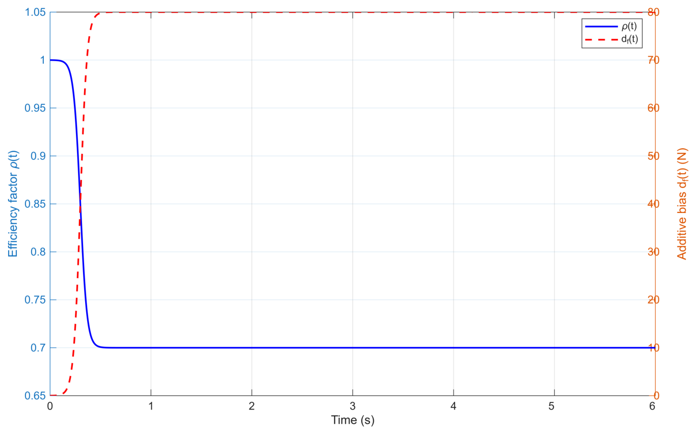
The actuator fault adopts a mixed fault model with both multiplicative efficiency loss and additive bias:

$$u_f\left(t\right)=\rho \left(t\right)u\left(t\right)+d_f\left(t\right)$$

$$s_f\left(t\right)={\displaystyle \frac{1}{1+\exp [-30(t-0.3\left)\right]}}$$

$$\rho \left(t\right)=1-0.3s_f\left(t\right),d_f\left(t\right)=80s_f\left(t\right)\mathrm{N}$$

where $s_f\left(t\right)$ is a sigmoid fault activation function that smoothly changes from 0 to 1 and is used to describe the transition from the fault-free state to the faulty state. The above setting indicates that the actuator experiences a smooth-transition mixed fault around $t=0.3$ s, where the efficiency gradually decreases from 1 to approximately 0.7 while an additive bias of about 80 N is generated. Since the passive suspension contains no active actuator, the actuator fault is applied only to the three active control schemes, APF, PID, and SMC. The actuator fault functions are shown in Figure 2.

6.2. Body Response Under Sinusoidal Road Excitation

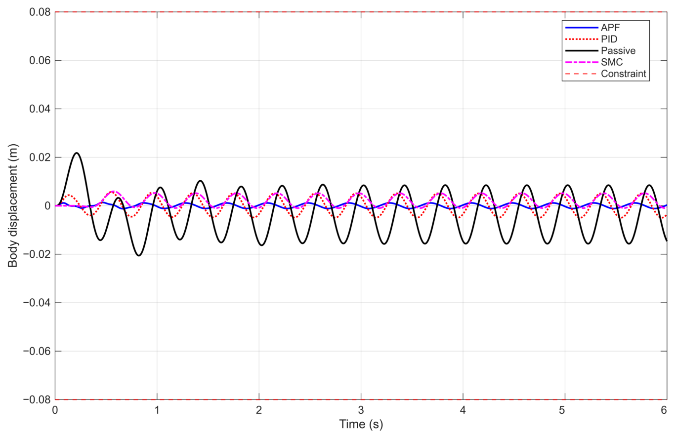
Figure 3 and Figure 4 show the body-displacement and body-acceleration responses under the four methods, respectively. As shown in Figure 3, the passive suspension produces a relatively large body displacement under sinusoidal road excitation, whereas PID and SMC suppress the vibration to some extent. The proposed method yields the smallest body-displacement amplitude, and the response always remains within the prescribed body-displacement constraint.

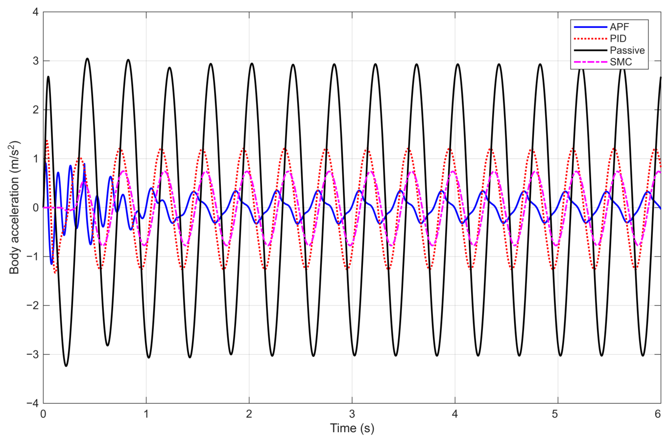
As shown in Figure 4, both the amplitude and overall fluctuation of the body acceleration under the proposed method are smaller than those under the comparison methods. Compared with the passive suspension, APF significantly reduces the vertical body acceleration. Compared with PID and SMC, APF still maintains a smoother acceleration response under the combined effects of actuator faults and suspension nonlinearities, demonstrating better improvement in ride comfort.

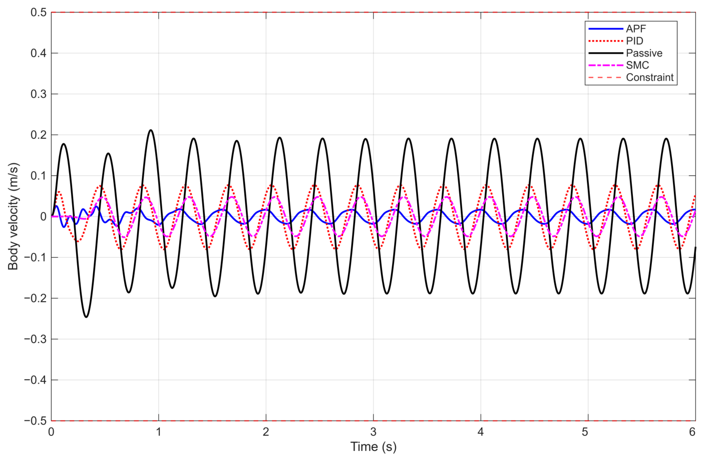
Figure 5 shows the body velocity response. The simulation results show that the body velocity under the proposed method always remains within the prescribed constraint bounds, and its fluctuation is smaller than those under the passive suspension and conventional feedback control methods.

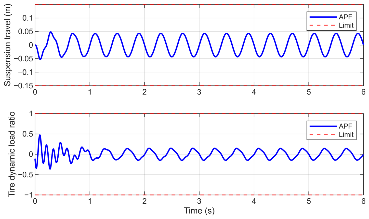
In addition to body comfort, active suspension control must also avoid excessive suspension travel and excessive tire dynamic load. Figure 6 shows that the suspension travel under APF control is always smaller than the mechanical travel limit, while the tire dynamic load ratio under APF control is always below the critical value. These results indicate that the proposed method improves body-displacement and acceleration responses without violating the suspension travel constraint or tire road holding safety.

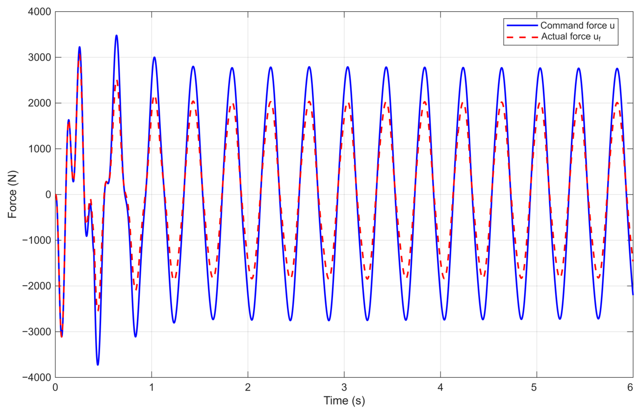
Figure 7 shows the command force of the APF controller and the actual actuator force after the fault. After the fault occurs, a deviation appears between the actual actuator force and the command force, reflecting the combined effects of actuator efficiency loss and additive fault. Even when the actual actuator force is degraded, the proposed APF method still maintains good suppression of body displacement and acceleration, indicating a certain fault-tolerant compensation capability.

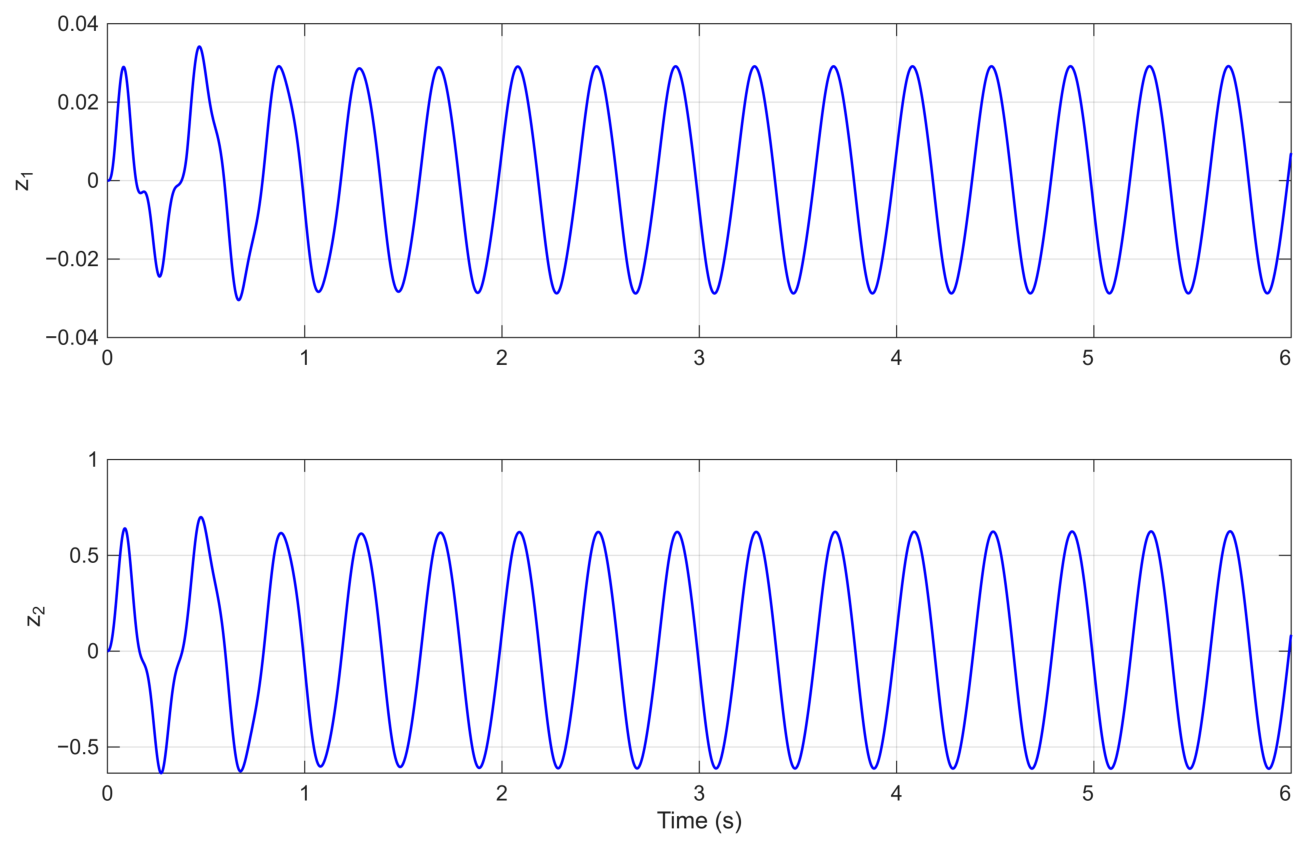
Figure 8 shows the time-domain responses of the transformed errors $z_1$ and $z_2$. Both errors remain bounded under the combined effects of sinusoidal road disturbance and mixed actuator fault.

6.3. Summary of Simulation Results

As shown in

Table 3. Quantitative performance comparison under sinusoidal road excitation and mixed actuator faults.

Method	Body-Displacement RMSE	RMS Body Acceleration	Control Energy
	(m)	($\mathrm{m}/{\mathrm{s}}^2$)	(${\mathrm{N}}^2\mathrm{s}$)
APF	0.000793	0.2579	$2.157\times {10}^7$
PID	0.003509	0.8696	$1.619\times {10}^7$
Passive	0.009707	2.1025	N/A
SMC	0.002951	0.5181	$1.298\times {10}^7$

, the proposed APF method achieves the smallest body-displacement RMSE and RMS body acceleration among the four suspension schemes. Compared with PID control, passive suspension, and SMC, the body-displacement RMSE is reduced by 77.39%, 91.83%, and 73.12%, respectively, while the RMS body acceleration is reduced by 70.34%, 87.73%, and 50.22%, respectively. The APF method requires higher cumulative control energy than PID and SMC, indicating a trade-off between improved ride comfort and control effort. Nevertheless, the body velocity, suspension travel, and tire dynamic load ratio remain within their prescribed safety ranges. Together with the command-force, actual-force, and transformed-error responses, these results demonstrate that the proposed method maintains bounded closed-loop signals and preserves the prescribed constraints in the presence of mixed actuator faults.

7. Conclusions

This paper applies the adaptive prescribed-time-filtered (APF) control method to a quarter-car nonlinear active suspension system with mixed actuator faults. Based on the strict-feedback suspension model, the displacement and velocity constraints of the sprung mass are handled through body-state constraint transformation; the unknown nonlinear function containing the additive fault is approximated online using an RBFNN; and an adaptive prescribed-time filter is introduced to alleviate the “explosion of complexity” in backstepping. Based on Lyapunov stability theory, the practical prescribed-time stability of the closed-loop system, preservation of body-state constraints, boundedness of the APF filtering error, and boundedness of the internal dynamics of the unsprung mass are proved. Sufficient conditions for satisfying the suspension travel and tire dynamic load constraints are also derived.

Numerical simulations verify the effectiveness of the proposed method. Under the combined action of sinusoidal road excitation and a smooth-transition actuator fault, APF is compared with passive suspension, PID, and SMC. The results show that APF outperforms the comparison methods in suppressing body displacement and attenuating acceleration, while the suspension travel and tire dynamic load do not exceed their safety bounds. In summary, the proposed APF method can achieve prescribed-time fault-tolerant constrained control for active suspension systems under simultaneous actuator faults and body-state constraints.

Future work will further explore the extension of the proposed framework to more intelligent and autonomous vehicle systems. Recent developments in autonomous perception, safety-aware decision-making, collaborative navigation, and human-in-the-loop learning provide broader perspectives for enhancing the adaptability and safety of control systems in complex environments [43,44,45,46]. Motivated by these advances, future studies will investigate integrated control architectures for active suspension systems operating under uncertain and complex conditions.

References

1. Hrovat, D. Survey of advanced suspension developments and related optimal control applications. Automatica 1997, 33, 1781–1817. [Google Scholar] [CrossRef] [Scilit]
2. Yamashita, M.; Fujimori, K.; Hayakawa, K.; Kimura, H. Application of H control to active suspension systems. Automatica 1994, 30, 1717–1729. [Google Scholar] [CrossRef] [Scilit]
3. Gao, H.; Sun, W.; Shi, P. Robust sampled-data H control for vehicle active suspension systems. IEEE Trans. Control Syst. Technol. 2010, 18, 238–245. [Google Scholar]
4. Sun, W.; Gao, H.; Kaynak, O. Finite frequency H control for vehicle active suspension systems. IEEE Trans. Control Syst. Technol. 2011, 19, 416–422. [Google Scholar]
5. Fialho, I.; Balas, G.J. Road adaptive active suspension design using linear parameter-varying gain-scheduling. IEEE Trans. Control Syst. Technol. 2002, 10, 43–54. [Google Scholar] [CrossRef] [Scilit]
6. Huang, T.; Pan, H.; Sun, W.; Gao, H. Sine resistance network-based motion planning approach for autonomous electric vehicles in dynamic environments. IEEE Trans. Transp. Electrif. 2022, 8, 2862–2873. [Google Scholar] [CrossRef] [Scilit]
7. Huang, T.; Pan, H.; Sun, W. A sensor fault detection, isolation, and estimation method for intelligent vehicles. Control Eng. Pract. 2023, 139, 105620. [Google Scholar] [CrossRef] [Scilit]
8. Hu, X.; Chen, H.; Ren, Q.; Gong, X.; Wang, P.; Hu, Y. Estimation and expansion of vehicle stability region with sums of squares programming. IEEE/ASME Trans. Mechatron. 2023, 28, 2820–2831. [Google Scholar] [CrossRef] [Scilit]
9. Deshpande, V.S.; Mohan, B.; Shendge, P.D.; Phadke, S.B. Disturbance observer based sliding mode control of active suspension systems. J. Sound Vib. 2014, 333, 2281–2296. [Google Scholar] [CrossRef] [Scilit]
10. Chen, S.A.; Wang, J.C.; Yao, M.; Kim, Y.B. Improved optimal sliding mode control for a nonlinear vehicle active suspension system. J. Sound Vib. 2017, 395, 1–25. [Google Scholar] [CrossRef] [Scilit]
11. Izci, D.; Ekinci, S.; Mohd Tumari, M.Z.; Ahmad, M.A. A novel softsign fractional-order controller optimized by an intelligent nature-inspired algorithm for magnetic levitation control. Fractal Fract. 2025, 9, 801. [Google Scholar]
12. Watanabe, M.; Prasad, A. Fractional delayed feedback for semi-active suspension control of nonlinear jumping quarter car model. Chaos Solitons Fractals 2025, 199, 116973. [Google Scholar] [CrossRef] [Scilit]
13. Zhao, W.; Gu, L. Adaptive PID controller for active suspension using radial basis function neural networks. Actuators 2023, 12, 437. [Google Scholar] [CrossRef] [Scilit]
14. Nguyen, T.A. Applying a PID-SMC synthetic control algorithm to the active suspension system to ensure road holding and ride comfort. PLoS ONE 2023, 18, e0283905. [Google Scholar] [CrossRef] [Scilit] [PubMed]
15. Ram, S.S.; Kumar, C.; Saravanakumar, R.; Banjerdpongchai, D. System identification and robust PID controller tuning of quarter car suspension system using hybrid optimization techniques. Sci. Rep. 2025, 15, 24195. [Google Scholar] [CrossRef] [Scilit] [PubMed]
16. Saat, S.; Ahmad, M.A.; Ghazali, M.R. Data-driven brain emotional learning-based intelligent controller-PID control of MIMO systems based on a modified safe experimentation dynamics algorithm. Int. J. Cogn. Comput. Eng. 2025, 6, 74–99. [Google Scholar]
17. Ghazali, M.R.; Ahmad, M.A.; Raja Ismail, R.M.T.; Tokhi, M.O. An improved neuroendocrine–proportional–integral–derivative controller with sigmoid-based secretion rate for nonlinear multi-input–multi-output crane systems. J. Low Freq. Noise Vib. Act. Control 2020, 39, 1172–1186. [Google Scholar]
18. Izci, D.; Ekinci, S.; Jabari, M.; Kocaman, B.; Gunes, B.B.; Adas, E.; Ahmad, M.A. A novel Gudermannian function-driven controller architecture optimized by starfish optimizer for superior transient performance of automatic voltage regulation. Biomimetics 2026, 11, 7. [Google Scholar] [PubMed]
19. Sun, W.; Pan, H.; Zhang, Y.; Gao, H. Multi-objective control for uncertain nonlinear active suspension systems. Mechatronics 2014, 24, 318–327. [Google Scholar] [CrossRef] [Scilit]
20. Pang, H.; Zhang, X.; Xu, Z. Adaptive backstepping-based tracking control design for nonlinear active suspension system with parameter uncertainties and safety constraints. ISA Trans. 2019, 88, 23–36. [Google Scholar] [CrossRef] [Scilit] [PubMed]
21. Pang, H.; Zhang, X.; Chen, J.; Liu, K. Design of a coordinated adaptive backstepping tracking control for nonlinear uncertain active suspension system. Appl. Math. Model. 2019, 76, 479–494. [Google Scholar] [CrossRef] [Scilit]
22. Huang, T.; Wang, J.; Pan, H. Adaptive bioinspired preview suspension control with constrained velocity planning for autonomous vehicles. IEEE Trans. Intell. Veh. 2023, 8, 3925–3935. [Google Scholar] [CrossRef] [Scilit]
23. Alleyne, A.; Hedrick, J.K. Nonlinear adaptive control of active suspensions. IEEE Trans. Control Syst. Technol. 1995, 3, 94–101. [Google Scholar]
24. Park, J.; Sandberg, I.W. Universal approximation using radial-basis-function networks. Neural Comput. 1991, 3, 246–257. [Google Scholar] [CrossRef] [Scilit] [PubMed]
25. Wang, F.; Xie, X.; Lv, Z.; Zhou, C. Adaptive neural network fixed-time fault-tolerant control of an uncertain nonlinear system with full-state constraints. Inf. Sci. 2022, 608, 858–880. [Google Scholar] [CrossRef] [Scilit]
26. Wu, L.B.; He, X.Q.; Guo, L.D.; Huang, S.J.; Hu, Y.H. Neural network adaptive switched fault-tolerant control of uncertain nonlinear systems with full state constraints. Neurocomputing 2024, 598, 128034. [Google Scholar] [CrossRef] [Scilit]
27. Tee, K.P.; Ge, S.S.; Tay, E.H. Barrier Lyapunov functions for the control of output-constrained nonlinear systems. Automatica 2009, 45, 918–927. [Google Scholar] [CrossRef] [Scilit]
28. Liu, Y.J.; Tong, S. Barrier Lyapunov functions for Nussbaum gain adaptive control of full state constrained nonlinear systems. Automatica 2017, 76, 143–152. [Google Scholar] [CrossRef] [Scilit]
29. Zhao, K.; Song, Y. Removing the feasibility conditions imposed on tracking control designs for state-constrained strict-feedback systems. IEEE Trans. Autom. Control 2019, 64, 1265–1272. [Google Scholar]
30. Cao, Y.; Song, Y.; Wen, C. Practical tracking control of perturbed uncertain nonaffine systems with full state constraints. Automatica 2019, 110, 108608. [Google Scholar] [CrossRef] [Scilit]
31. Li, H.; Gao, H.; Liu, H.; Liu, M. Fault-tolerant H control for active suspension vehicle systems with actuator faults. Proc. Inst. Mech. Eng. Part I J. Syst. Control Eng. 2012, 226, 348–363. [Google Scholar]
32. Kazemipour, A.; Novinzadeh, A.B. Adaptive fault-tolerant control for active suspension systems based on the terminal sliding mode approach. Proc. Inst. Mech. Eng. Part C J. Mech. Eng. Sci. 2020, 234, 501–511. [Google Scholar]
33. Guo, X.; Wang, J.; Sun, W. Nonlinear adaptive fault-tolerant control for full-car active suspension with velocity measurement errors and full-state constraints. J. Frankl. Inst. 2024, 361, 106845. [Google Scholar]
34. Huang, T.; Wang, J.; Pan, H.; Sun, W. Finite-time fault-tolerant integrated motion control for autonomous vehicles with prescribed performance. IEEE Trans. Transp. Electrif. 2023, 9, 4255–4265. [Google Scholar] [CrossRef] [Scilit]
35. Wang, K.; Liu, X.; Jing, Y. Command filtered finite-time control for nonlinear systems with state constraints and its application to TCP network. Inf. Sci. 2021, 550, 189–206. [Google Scholar] [CrossRef] [Scilit]
36. Wu, Z.; Zhang, T.; Xia, X.; Yi, Y. Finite-time adaptive neural command filtered control for pure-feedback time-varying constrained nonlinear systems with actuator faults. Neurocomputing 2022, 490, 193–205. [Google Scholar]
37. Jiang, S.; Shen, H.; Dong, L.; Zhi, S.; Ren, F.; Liu, J. Prescribed-time command filtered control for a class uncertain nonlinear systems. ISA Trans. 2024, 152, 229–237. [Google Scholar] [CrossRef] [Scilit] [PubMed]
38. Wang, F.; Gao, Z.; Xie, X.; Zhou, C.; Hua, C. Adaptive prescribed-time filtered control design for a full-state constrained nonlinear system. IEEE Trans. Cybern. 2025, 55, 321–331. [Google Scholar] [CrossRef] [Scilit] [PubMed]
39. Huang, T.; Wang, J.; Pan, H. Approximation-free prespecified time bionic Reliable control for vehicle suspension. IEEE Trans. Autom. Sci. Eng. 2024, 21, 5333–5343. [Google Scholar]
40. Gao, H.; Lam, J.; Wang, C. Multi-objective control of vehicle active suspension systems via load-dependent controllers. J. Sound Vib. 2006, 290, 654–675. [Google Scholar] [CrossRef] [Scilit]
41. Du, H.; Lam, J.; Sze, K.Y. Design of non-fragile H controller for active vehicle suspensions. J. Vib. Control 2005, 11, 225–243. [Google Scholar] [CrossRef] [Scilit]
42. Hu, X.; Wang, P.; Cai, S.; Zhang, L.; Hu, Y.; Chen, H. Vehicle stability analysis by zero dynamics to improve control performance. IEEE Trans. Control Syst. Technol. 2023, 31, 2365–2379. [Google Scholar] [CrossRef] [Scilit]
43. Vinodha, K.; Gopi, E.S.; Agnibhoj, T. LiDAR-based estimation of bounding box coordinates using Gaussian process regression and particle swarm optimization. Biomim. Intell. Robot. 2024, 4, 100140. [Google Scholar]
44. Sellers, T.; Lei, T.; Luo, C.; Bi, Z.; Jan, G.E. Human autonomy teaming-based safety-aware navigation through bio-inspired and graph-based algorithms. Biomim. Intell. Robot. 2024, 4, 100189. [Google Scholar] [CrossRef] [Scilit]
45. Chen, W.; Chi, W.; Ji, S.; Ye, H.; Liu, J.; Jia, Y.; Yu, J.; Cheng, J. A survey of autonomous robots and multi-robot navigation: Perception, planning and collaboration. Biomim. Intell. Robot. 2025, 5, 100203. [Google Scholar] [CrossRef] [Scilit]
46. Oriyama, M.; Hartono, P.; Sawada, H. Human-in-the-loop transfer learning in collision avoidance of autonomous robots. Biomim. Intell. Robot. 2025, 5, 100215. [Google Scholar] [CrossRef] [Scilit]
Figure 1. Quarter-Car Active Suspension Model.
Electronics 15 02835 g001
Figure 2. Actuator fault functions.
Electronics 15 02835 g002
Figure 3. Comparison of body-displacement responses.
Electronics 15 02835 g003
Figure 4. Comparison of body-acceleration responses.
Electronics 15 02835 g004
Figure 5. Comparison of body velocity responses.
Electronics 15 02835 g005
Figure 6. Suspension safety responses: suspension travel (top) and tire dynamic load ratio (bottom).
Electronics 15 02835 g006
Figure 7. APF command force and actual actuator force.
Electronics 15 02835 g007
Figure 8. Transformed error responses.
Electronics 15 02835 g008