Abstract
In recent times, 3D eye tracking methods have been actively studied to utilize gaze information in various applications. As a result, there is growing interest in gaze depth estimation techniques. This study introduces a monocular method for estimating gaze depth using DPI distance and pupil size. We acquired right eye images from eleven subjects and at ten gaze depth levels ranging from 15 cm to 60 cm at intervals of 5 cm. We used a camera equipped with an infrared LED to capture the images. We applied a contour-based algorithm to detect the first Purkinje image and pupil, then used a template matching algorithm for the fourth Purkinje image. Using the detected features, we calculated the pupil size and DPI distance. We trained a multiple linear regression model on data from eight subjects, achieving an R2 value of 0.71 and a root mean squared error (RMSE) of 7.69 cm. This result indicates an approximate 3.15% reduction in error rate compared to the general linear regression model. Based on the results, we derived the following equation: depth fixation = 20.746 × DPI distance + 5.223 × pupil size + 16.495 × (DPI distance × pupil size) + 13.880. Our experiments confirmed that gaze depth can be effectively estimated from monocular images using DPI distance and pupil size.
1. Introduction
Gaze contains a great of information. Recently, many industries have adopted eye-tracking technologies to make use of gaze-related data. Previously, most content was designed for 2D displays. Consequently, earlier research focused primarily on 2D coordinate tracking. A notable study in 2D eye tracking revealed differences in horizontal and vertical saccades among patients with Alzheimer’s disease, amnestic mild cognitive impairment, and healthy older adults [1]. The authors indicated that eye movement latency could be used to identify signs of pathological aging. Raney et al. [2] studied the cognitive process of reading comprehension using gaze tracking and outlined the benefits of using eye movements. They found that such movements reflect both the textual features and the reader’s individual characteristics. Furthermore, they can facilitate reading analysis not only at the level of full texts but also at the level of smaller units such as words. Because the display distance was constant, these studies did not require gaze depth estimation. Advances in technology have resulted in the emergence of diverse 3D content, including VR and AR. This has led to an increase in research on 3D eye tracking incorporating gaze depth. In [3], the authors mentioned a museum assistant that employs eye tracking to identify which artworks visitors are interested in and provide appropriate feedback. Alt et al. [4] used gaze tracking as a method of interacting with 3D interfaces. They compared the results of two different methods for estimating gaze depth in a 3D game, namely, pupil size and pupil distance. These papers have noted that eye tracking can be useful when the display is distant or dirty, making touch input difficult [3,4]. As the demand for 3D eye tracking has grown, so has interest in easily and accurately estimating gaze depth. Most previous studies were based on binocular methods. In this paper, we propose a monocular method for estimating gaze depth based on DPI distance and pupil size. A Purkinje image is a reflected image of the light entering the eye [5]. DPI refers to the first and fourth Purkinje images. We conducted experiments to measure changes in DPI distance and pupil size with respect to gaze depth, analyzed their relationships statistically, and derived an equation. The contributions of this study can be summarized as follows:
- Monocular Based MethodMany existing studies rely on binocular methods. In contrast, our approach uses monocular images to estimate gaze depth even in environments where binocular information is unavailable.
- Various Gaze Depth RangesWe set the gaze depth range from 15 cm to 60 cm at intervals of 5 cm. Compared to previous studies, this setup provides a broader and more detailed range, enabling us to observe changes in ocular features corresponding to small variations in gaze depth.
- Low-Cost MethodWhile most previous eye tracking studies require capturing the information of both eyes, we estimate gaze depth by capturing the information of just one eye using a single camera. This approach reduces both computational complexity and cost.
The above contributions are detailed in the Section 4. The remainder of this paper is organized as follows: Section 2 reviews related work on eye tracking with a focus on gaze depth estimation, and highlights how our approach differs; Section 3 describes the features and images used to estimate gaze depth along with the feature extraction algorithm and analysis method; Section 4 presents the experimental design and results; in Section 5, we compare the performance of our method with existing binocular based approaches; finally, Section 6 concludes the paper with a discussion of limitations and future work.
2. Related Work
There are various methods for eye tracking that can be grouped into distinct categories. Here, we categorize eye tracking research into binocular and monocular approaches, first describing research on binocular gaze estimation followed by research on monocular gaze estimation. Binocular methods estimate gaze depth using data from both eyes, while monocular based methods rely on data from a single eye. At the end of this section, we compare our proposed method with existing approaches and highlight their differences.
2.1. Binocular Gaze Tracking
Arefin et al. [6] studied the estimation of perceived depth changes in VR with gaze tracking. They utilized the HTC VIVE Pro with an integrated Tobii eye tracker to measure changes in interpupillary distance (IPD) and eye vergence angle (EVA) with respect to depth. EVA is the angle between the visual axes of the eyes [7], while IPD is the distance between the centers of the pupils [8]. For near objects, EVA increases and IPD decreases as the eyes converge inward. For distant objects, EVA decreases and IPD increases as the eyes diverge outward [6]. As hypothesized, the experimental results showed that EVA and IPD changed with perceptual depth and that the degree of change in these features reflected the variations in perceptual depth. Stevenson et al. [9] attempted to estimate 3D gaze using electrooculography (EOG). When the eye rotates, its dipole moment changes, resulting in a change in the measured EOG voltage. Consequently, this voltage change can be used to estimate eye movements. They used eight external electrodes attached around the eyes. The results showed that the linear model achieved an average fixation distance error of 13.40 ± 11.80% (7.50 ± 5.60 cm), while the neural network model achieved 10.30 ± 10.00% (5.70 ± 4.70 cm). Another study estimated gaze depth using gaze normal vectors, which are 3D vectors that represent the direction in which the eye is looking [10]. The depth distance was set to range from 1 to 5 m at intervals of 1 m, and an eye tracker from Pupil Labs was used to obtain the gaze vectors [11]. The MLP classification and regression models achieved an average classification error rate of 9.92 ± 10.55% and an average error distance of 0.42 ± 0.23 m, respectively. Wang et al. [12] proposed a new interface called FocusFlow which actively utilizes gaze depth. They conducted a pilot study on gaze depth estimation for system design. The intersection of gaze rays from both eyes was used to estimate the gaze depth. In this case, the gaze rays were projected onto the x- and z-axes to prevent errors in the intersection point caused by gaze angle inaccuracies. Using the built-in eye tracker of the HTC VIVE Pro Eye headset, they employed fixed targets at depths of 0.5, 1.0, and 2.0 m as well as moving targets between 0.5 and 2.5 m. The results showed that estimation was relatively accurate at short distances but became less accurate at longer distances. Li et al. [13] proposed MSMI-Net, an architecture for 3D eye tracking. MSMI-Net consists of a stream that extracts high-dimensional features from the right and left eye images and another that extracts and fuses low-dimensional features from eye and face images. The result is a 2D vector that can be transformed into a 3D gaze direction using a specific equation. The authors conducted performance experiments on three datasets. Unfortunately, the methods presented in this section cannot be applied when binocular images are not available. Thus, we propose a monocular gaze depth estimation method as an alternative to binocular methods.
2.2. Monocular Gaze Tracking
Mardanbegi et al. [14] studied gaze depth estimation based on the vestibulo-ocular reflex (VOR) gain in VR. VOR refers to the compensatory eye movement during head rotation, and the VOR gain is the ratio of the eye’s angular velocity to the head’s angular velocity. The VOR gain varies with the distance between the eye and the target, which can be used to estimate the gaze depth. Their experiment was conducted using an HTC Vive virtual reality setup integrated with a Tobii eye tracker. The results showed that VOR gain and vergence varied similarly with gaze depth. Mansouryar et al. [15] attempted monocular gaze tracking using an eye camera and a scene camera. They mapped the 2D pupil position from the eye camera to the 3D gaze direction from the scene camera (2D-to-3D method). The performance of the proposed method was compared with existing 2D-to-2D and 3D-to-3D methods. The gaze distance was set from 1 to 2 m in intervals of 25 cm and data were collected with a PUPIL head-mounted eye tracker [11]. The 2D-to-2D method maps the 2D pupil position from the eye camera to the 2D gaze position of the scene camera, while the 3D-to-3D method estimates the 3D pupil position from the eye camera and directly maps it to the 3D gaze vector of the scene camera [15]. Their results showed that the 2D-to-3D method outperformed the 2D-to-2D method in simulated environments and the 3D-to-3D method on real-world data. In [16], a method was presented for mapping 3D positions obtained using fiducial markers to pupil positions obtained from an eye camera. Fiducial markers were embedded in 3D objects and captured by a world camera to obtain their 3D coordinates. The experiment used a Stanford bunny as the target with five marked target points, and acquired eye features with a Pupil eye tracker [11]. As a result, an average depth error of 7.71 mm was achieved at a target distance of 553.97 mm. The previous two studies are similar to ours in that they use monocular eye images; however, they require two cameras to capture the eye images, while our study uses only one camera.
2.3. Differences from Previous Studies
In this section, we discuss the differences between our work and previous studies. First, unlike most existing studies, we employ a monocular method that remains applicable even when binocular images are unavailable. Second, we set the gaze depth from 15 cm to 60 cm at intervals of 5 cm, allowing us to observe the effect of smaller changes in gaze depth compared to previous studies. Third, the VOR-based method requires subjects to move their heads while fixating on the target to obtain VOR gain, which some subjects may find difficult. In fact, some subjects in [14] had difficulty maintaining fixation during head movements and were excluded from the data analysis. Fourth, while the EOG-based method offers the advantages of low cost and insensitivity to lighting conditions [9], it requires electrodes to be directly attached to the subject, which may cause discomfort and complicate data collection. In this study, we use a noncontact method to record the eye when the subject is looking at the target, resulting in reduced effort and discomfort during the experiment. Finally, some monocular methods require two cameras to capture both eye and scene images. In contrast, we use a single camera with an infrared LED and estimate gaze depth using only eye images.
3. Methods
This section introduces our experimental methodology. First, we briefly describe the overall experimental process. Next, we explain the Purkinje and pupil images used as features for gaze tracking along with their relationship to gaze depth. We then provide a detailed description of the eye images and feature detection algorithms that we used. Finally, we provide a brief overview of the methods used in our analysis.
3.1. Proposed Methods
The experimental procedure for analyzing the relationship among gaze depth, DPI distance, and pupil size was as follows. First, we acquired eye images from eleven subjects at ten different depth levels. The proposed algorithm was then applied to the eye images to extract the pupil image and DPI, which were used to calculate the pupil size and DPI distance. These values were used to perform regression and correlation analyses. Finally, their relationships are defined in an equation. This study contributes to research on 3D gaze estimation by experimentally demonstrating how DPI distance and pupil size change with gaze depth.
3.2. Purkinje Image
A Purkinje image is formed by the reflection of light from the internal structures of the eye. The first, second, third, and fourth Purkinje images are formed by the anterior and posterior surfaces of both the cornea and the lens. The first Purkinje image is relatively large and bright, making it easier to detect than the others. In contrast, the second and third Purkinje images are obscured by the first, making them difficult to detect. The fourth Purkinje image is relatively easy to detect because it has a different position than the others [5]. The first and fourth Purkinje images are called dual Purkinje images (DPI); in this paper, we estimate the gaze depth using the DPI distance. The eye adjusts the thickness of the lens to focus on changing depth distances, which affects the position of the fourth Purkinje image. Focusing on a close object reduces the DPI distance because the lens becomes thicker, whereas focusing on a distant object increases the DPI distance because the lens becomes thinner [17]. Figure 1 shows the change in lens thickness as a function of the target distance. We hypothesize that changes in DPI distance can be used to estimate gaze depth, and analyze the correlation between DPI distance and gaze depth through our experiments.
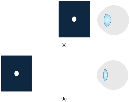
Figure 1.
Change in lens thickness with depth levels: (a) when focusing on a nearby object and (b) when focusing on a distant object.
3.3. Pupil Size
Pupil size is known to vary depending on various factors, including illumination conditions, gaze depth, and psychological state [18]. In bright environments, the pupil contracts to reduce the amount of incoming light, whereas in dim environments, it dilates to allow more light in. Additionally, the pupil is relatively constricted at closer distances and dilated at farther distances. Figure 2 illustrates the change in pupil size with respect to target distance. Pupil size can also change in response to psychological states. A study by Lee et al. [19] found significant changes in pupil diameter related with the emotions of fear, anger, and surprise. In this study, we analyze the correlation between pupil size and gaze depth while minimizing the influence of external factors on pupil size.
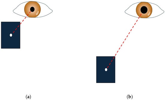
Figure 2.
Change in pupil size with depth levels: (a) when focusing on a nearby object and (b) when focusing on a distant object.
3.4. Eye Images
Eye images are required in order to extract the pupil and Purkinje images. In our experiments, we recorded eye videos of approximately seven seconds for each gaze depth. Five eye images were extracted from each video by selecting frames with a clear Purkinje image. These images were cropped to 400 px in width and 260 px in height based on the coordinates specified for each subject, referred to as the region of interest (ROI). The pupil area was detected by applying an algorithm to the ROI. For Purkinje image detection, a Purkinje image region of interest (PROI) was used. PROIs were generated by cropping the ROI based on the pupil center, resulting in a width of 150 px and a height of either 100, 120, 160, or 170 px. Figure 3 shows an example of the PROI and ROI used in our experiment. The pupil size image and first Purkinje image were detected using contour-based algorithms, while the fourth Purkinje image was detected using a template matching-based algorithm. Three images were used for training and two for testing. Image processing and feature detection were implemented using Visual Studio 2022, C++, and OpenCV version 4.0.0.
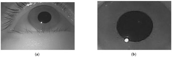
Figure 3.
Example images for experiments: (a) ROI and (b) PROI.
3.5. Pupil Size Detection Method
Pupil size detection was based on the method used in the visual fatigue assessment study reported in [20]. For pupil detection, blurring and binarization operations were applied sequentially to the ROI. The blurring kernel size was set to 5 × 5 and the binarization threshold to 55, 60, or 80 depending on the subject. The contour detection algorithm was then applied to the preprocessed ROI. To detect the contour corresponding to the pupil, the area and perimeter length were calculated only if a parent contour existed. When these values met the criteria, the convex hull algorithm was applied to extract a convex polygon. If the convex polygon contained at least a certain number of points, the ellipse estimation algorithm was executed. We settled on a threshold of either 20 or 30 points depending on the subject. The estimated ellipse was used represent the pupil, with its length considered as the pupil size. The calculated pupil size was measured in pixels (px). The result of drawing a bounding box around the pupil area is shown in (f) in Figure 4.

Figure 4.
Pupil detection process: (a) ROI, (b) blurred ROI, (c) binarized ROI, (d) detected contour, (e) detected ellipse, (f) detected bounding box.
3.6. First Purkinje Image Detection Method
To calculate the DPI distance, the center coordinates of each Purkinje image must be estimated. The first Purkinje image was detected using a contour-based method similar to the one used for pupil detection. For preprocessing, binarization was applied to the PROI, with the threshold set to 220. After applying the contour detection algorithm to the binarized image, the circularity, area, and perimeter of each contour were calculated. If these values met the criteria, the convex hull algorithm was applied to detect convex polygons. If the polygon contained five or more points, it was assumed to represent the first Purkinje image and the ellipse estimation algorithm was applied. This ellipse was defined as the first Purkinje image and its center coordinates were set to those of the first Purkinje image. The process of detecting the first Purkinje image is illustrated in Figure 5.
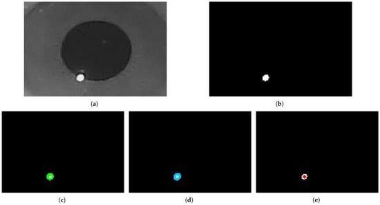
Figure 5.
First Purkinje image detection process: (a) PROI, (b) binarized PROI, (c) detected contour, (d) detected ellipse, (e) detected center of the first Purkinje image.
3.7. Fourth Purkinje Image Detection Method
Compared to the first Purkinje image, the fourth Purkinje image is smaller and darker, making it more difficult to detect using contour-based methods. We employed a template matching algorithm to detect the fourth Purkinje image [21]. For each subject, the fourth Purkinje image was extracted from the eye image and used as a template. After applying the template-matching algorithm to the PROI, we located the coordinates of the maximum value in the resulting matrix. The calibrated center coordinates of the ellipse were then considered as the center coordinates of the fourth Purkinje image. Figure 6 shows examples of the fourth Purkinje image detection and the template image.
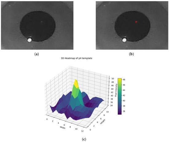
Figure 6.
Fourth Purkinje image detection process: (a) PROI, (b) detected center of the fourth Purkinje image, (c) 3D heatmap of the fourth Purkinje image template.
3.8. DPI Distance Calculation
The DPI distance was calculated as the Euclidean distance between the center coordinates of the Purkinje images using Equation (1), where and represent the center coordinates of the first Purkinje image and and represent the center coordinates of the fourth Purkinje image. The resulting DPI distance is expressed in px.
3.9. Analysis Method
We performed graph, correlation, and regression analyses to investigate the relationships between gaze depth, DPI distance, and pupil size. Graph analysis provided visual representations of the relationships between variables using a 2D scatter plot. Correlation analysis allowed us identify the correlations between variables and compare the p-values to determine whether the relationships were statistically significant. In the regression analysis, we trained linear, logistic, and multiple linear regression models for each subject, then evaluated the models in terms of their predictive performance and fit. Finally, we trained models using data from all subjects and represented the relationships as a mathematical equation. The analyses were performed using Visual Studio 2022, Python version 3.8.5, SciPy version 1.5.4, and Scikit-learn version 0.23.2.
4. Experimental Results
The following section presents the experimental design used in this study. We measured variations in DPI distance and pupil size with different gaze depths in eleven subjects. A camera with an infrared LED was used to generate a Purkinje image and record the right eye. We used hardware with the following specifications:
- Camera model: Logitech C600 (Lausanne, Switzerland), recording at 30 frames per second (fps).
- Camera magnification: Ranging from 15 to 17 px/mm.
- Infrared illumination: LED with a wavelength of 900 nm.
We fixed the distance between the eye and the camera at 4–5 cm and captured eye images at a resolution of 1280 × 720. The target distances were set from 15 to 60 cm with 5 cm intervals. These distances were selected to cover a wide range based on previous studies [17,18,22], with the shortest distance adjusted to 15 cm to accommodate the experimental setup. We placed the head-and-chin rest and the target in calibrated positions so that the eyes were aligned with the target. This setup was designed to minimize eye rotation based on the target distance. The target consisted of a piece of black paper with a white sticker attached to it, which was secured in a paper holder. Figure 7 illustrates the experimental setup. We restricted the experimental environment to allow only one subject at a time, and minimized light interference by using curtains to block external light and turning off all interior lighting. There were eleven subjects (five males) with an average age of 28.4 ± 6.7 years. The experiment was conducted on adults with normal vision (including corrected-to-normal vision) with the exception of one nearsighted subject. All subjects provided written informed consent and were fully informed about the experiment before participating.
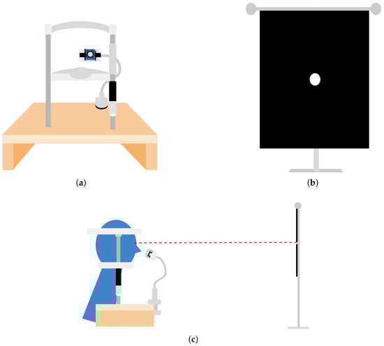
Figure 7.
Experimental setup: (a) head-and-chin rest and camera setup, (b) target used in the experiment, and (c) example showing experimental equipment in use.
The experiment was conducted as follows. First, the subjects were informed about the procedures and precautions. They were then asked to provide their age, sex, and visual acuity and to sign an informed consent form. Second, the subjects sat in a chair and positioned their heads on a head-and-chin rest mounted on the desk. The experimenter ensured that each subject’s eye was properly captured by the camera. Third, the subjects fixated on a target in front of them for seven seconds while their right eye was recorded. After seven seconds, the experimenter moved the target to the next distance. This process was repeated for all gaze depths.
In our experiments, both the DPI distance and pupil size were detected for only eight (four males) out of eleven subjects, including the one myopic subject (Subject 11). The average age for these eight subjects was 28.1 ± 7.0 years. The reason for the missing data was that the fourth Purkinje image was not detected in the other subjects. For certain data, we performed feature detection manually. Because the intensity of the infrared LED was accidentally changed during the experiment, the data from two subjects (Subjects 1 and 2) were collected under a different LED condition. Our graph, correlation, and regression analyses were performed with this in mind.
4.1. Graph Analysis
We plotted a 2D scatter plot for each of the depth fixation, DPI distance, and pupil size. The following scatter plots illustrate the relationships between DPI distance and depth fixation, pupil size and depth fixation, and DPI distance and pupil size for each subject (Figure 8). Depth fixation is measured in cm, while DPI distance and pupil size are measured in px.

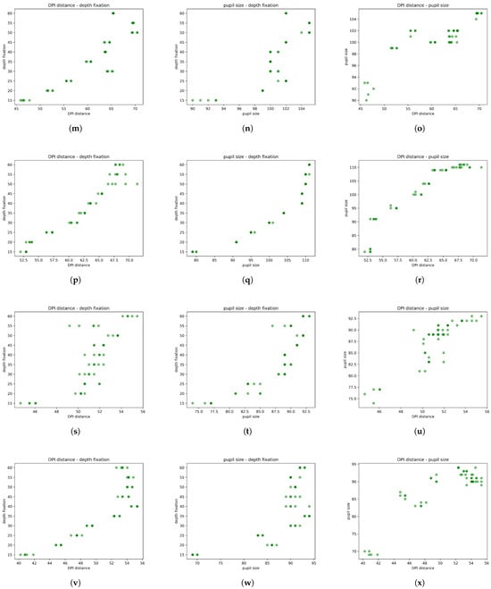
Figure 8.
Graphs for Subjects 1, 2, 4, 5, 7, 8, 10, and 11 are shown in the order listed above. (a,d,g,j,m,p,s,v): DPI distance vs. depth fixation, (b,e,h,k,n,q,t,w): pupil size vs. depth fixation, (c,f,i,l,o,r,u,x): DPI distance vs. pupil size, along with their corresponding graphs and equations (The darker areas of the points indicate regions where data points with the same value overlap, resulting in visually stronger colors).
The scatter plots show that the DPI distance and pupil size tended to increase as the depth fixation increased. Additionally, the scatter plot of DPI distance vs. pupil size indicates that an increase in one variable tends to be associated with an increase in the other. To statistically quantify their relationships, a correlation analysis was conducted between the variables.
4.2. Correlation Analysis
To analyze the correlations between the variables, we used Spearman’s rank correlation, which is a nonparametric method for assessing correlation based on variable rankings. A correlation coefficient close to 1 indicates a positive correlation between variables, while a coefficient close to −1 indicates a negative correlation. A value near 0 suggests no correlation between the variables. The results of our analysis for each subject are presented in the following table (Table 1).

Table 1.
Spearman’s rank correlation results for Subjects 1, 2, 4, 5, 7, 8, 10, and 11 (The bold numbers represent the minimum values for each column.)
For all subjects, the correlation between DPI distance and depth fixation was greater than or equal to 0.32, with p-values below 0.05 (5%), indicating a statistically significant positive correlation. We also observed correlations greater than or equal to 0.36 for pupil size and depth fixation and greater than or equal to 0.31 for DPI distance and pupil size (p < 0.05). For subjects 4, 8, and 10, the correlation between pupil size and depth fixation was higher than that between DPI distance and depth fixation. The correlation between DPI distance and depth fixation was stronger for the remaining subjects. We examined the relationship between these correlation coefficients and the actual predictive performance of the model in a regression analysis. In conclusion, all variables showed a statistically significant positive correlation with each other across all subjects.
4.3. Regression Analysis Based on Individual Subject Data
4.3.1. Linear Regression Analysis
In the previous section, a positive correlation between the variables was observed using Spearman’s correlation. In this section, we model the relationships between the variables using regression. First, a linear regression model was applied. The following graphs illustrate the results of the analysis (Figure 9).


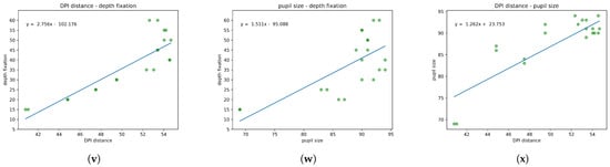
Figure 9.
Graphs for Subjects 1, 2, 4, 5, 7, 8, 10, and 11 are shown in the order listed above. (a,d,g,j,m,p,s,v): DPI distance vs. depth fixation, (b,e,h,k,n,q,t,w): pupil size vs. depth fixation, (c,f,i,l,o,r,u,x): DPI distance vs. pupil size, along with their corresponding graphs and equations (The darker areas of the points indicate regions where data points with the same value overlap, resulting in visually stronger colors).
To evaluate the performance of the regression model, we used the R-squared (R2) and root mean squared error (RMSE) indicators. The R2 value indicates how well the model explains the variance, and is used to assess its fit. Values close to 1 indicate a good fit, while those close to 0 indicate a poor fit. The RMSE is the square root of the mean squared difference between the actual values and the values predicted by the regression model. It represents the error in the original units of the data, and is used to assess the predictive performance of the model. The table below summarizes the R2 and RMSE results (Table 2). RMSE is measured in cm for DPI distance vs. depth fixation, cm for pupil size vs. depth fixation, and px for DPI distance vs. pupil size.
Table 2.
R2 and RMSE for linear regression of Subjects 1, 2, 4, 5, 7, 8, 10, and 11.
Comparing the RMSE and R2 values, it can be seen that DPI distance-based gaze depth estimation achieved better performance in linear regression for subjects 4 and 8, despite the higher correlation between pupil size and depth fixation. In contrast, the pupil size-based model outperformed the model based on DPI distance for subject 10. These results indicate that a stronger correlation does not necessarily lead to better predictive performance.
4.3.2. Normalized Linear Regression Analysis
DPI distance and pupil size vary across subjects, which can be attributed to individual characteristics as well as to external factors such as changes in LED intensity. To eliminate these differences, we normalized the DPI distance and pupil size to a range between 0 and 1 for each subject using min–max scaling, then performed linear regression again. The following graphs illustrate the normalized linear model (Figure 10).


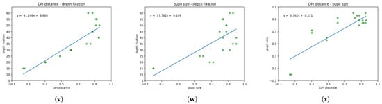
Figure 10.
Graphs for Subjects 1, 2, 4, 5, 7, 8, 10, and 11 are shown in the order listed above. (a,d,g,j,m,p,s,v): DPI distance vs. depth fixation, (b,e,h,k,n,q,t,w): pupil size vs. depth fixation, (c,f,i,l,o,r,u,x): DPI distance vs. pupil size, along with their corresponding graphs and equations (The darker areas of the points indicate regions where data points with the same value overlap, resulting in visually stronger colors).
The table below summarizes the R2 and RMSE results (Table 3).
Table 3.
R2 and RMSE for normalized linear regression of Subjects 1, 2, 4, 5, 7, 8, 10, and 11.
After performing linear regression on the normalized data, the RMSE for DPI distance and pupil size was 0.24 or lower for all subjects. The input data for all subsequent regressions were also normalized to a range of 0 to 1.
4.3.3. Logistic Regression Analysis
A logistic regression model was used for the nonlinear regression analysis. The results of the logistic model are shown in Figure 11 and Table 4. When plotting the regression graph, values were divided into 100 bins between 0 and 1 and used as input.

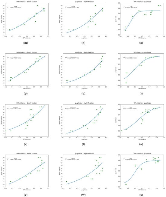
Figure 11.
Graphs for Subjects 1, 2, 4, 5, 7, 8, 10, and 11 are shown in the order listed above. (a,d,g,j,m,p,s,v): DPI distance vs. depth fixation, (b,e,h,k,n,q,t,w): pupil size vs. depth fixation, (c,f,i,l,o,r,u,x): DPI distance vs. pupil size, along with their corresponding graphs and equations (The darker areas of the points indicate regions where data points with the same value overlap, resulting in visually stronger colors).
Table 4.
R2 and RMSE for logistic regression of Subjects 1, 2, 4, 5, 7, 8, 10, and 11.
Compared to the normalized linear regression results, the logistic regression achieved equal or better performance across all metrics, except for DPI distance and depth fixation in Subject 5. Therefore, the logistic model more effectively represented the data than the linear model.
4.3.4. Multiple Linear Regression Analysis
Thus far, we have analyzed the one-to-one relationships between the variables. In this section, we investigate how using both DPI distance and pupil size affects depth estimation. To investigate this, a multiple linear regression was conducted with DPI distance and pupil size as independent variables and depth fixation as the dependent variable. In order to focus on the relationship analysis, the regression was performed using the model y = a + b + c + d, excluding the quadratic term. Here, y, , and represent the depth fixation, DPI distance, and pupil size, respectively. The graphs of the multiple linear regression results are shown below (Figure 12).

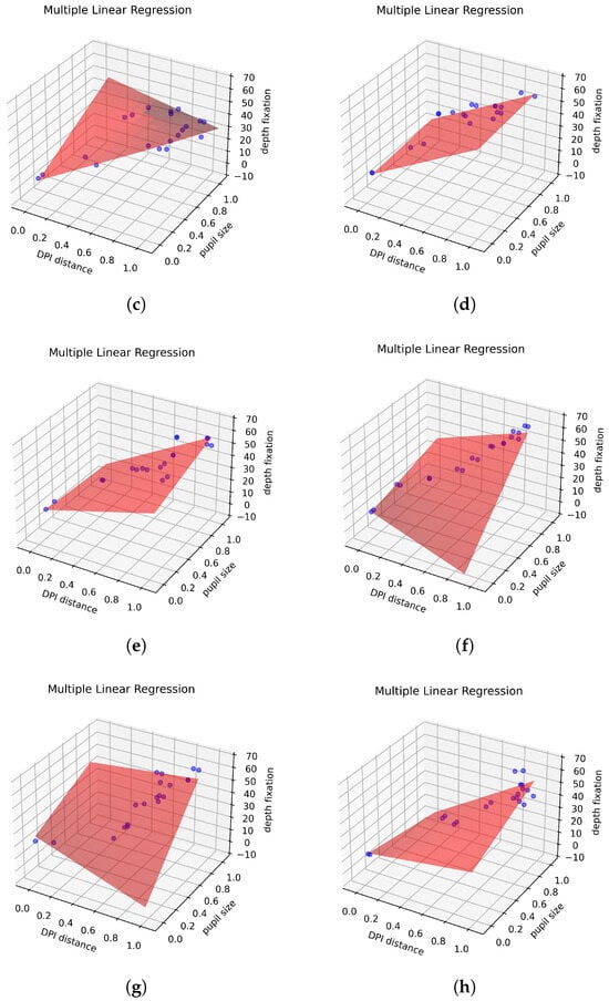
Figure 12.
Graphs for multiple linear regression: (a) Subject 1, (b) Subject 2, (c) Subject 4, (d) Subject 5, (e) Subject 7, (f) Subject 8, (g) Subject 10, and (h) Subject 11 (The darker areas of the points indicate regions where data points with the same value overlap, resulting in visually stronger colors).
The following table summarizes the R2 and RMSE results along with the corresponding regression equations for the multiple linear regression (Table 5).
Table 5.
R2, RMSE, and regression equations for multiple linear regression of Subjects 1, 2, 4, 5, 7, 8, 10, and 11.
The multiple linear model achieved an equal or higher R2 and lower RMSE compared to the linear model when using either the DPI distance or pupil size alone. In particular, the RMSE decreased from 7.20 to 6.09 for Subject 10, which represents a significant improvement compared to the results for the other subjects. Compared to the logistic model, the multiple linear regression model performed better for subjects 2, 5, and 8, whereas the logistic model outperformed the multiple linear model for subjects 1, 7, and 11. For subject 4, both models achieved the same level of performance. For Subject 10, the multiple linear model outperformed the logistic model based on DPI distance but underperformed the logistic model based on pupil size. Unlike the other subjects, Subject 10 performed better with pupil size than with DPI distance, which may have influenced the results. These experimental results show that considering both DPI distance and pupil size together leads to better predictive performance than the linear model and more stable performance than the logistic model.
4.4. Regression Analysis Based on Overall Data
4.4.1. Generalized Normalized Linear Regression Analysis
Previously, we trained separate models for each subject and analyzed the results. Next, we trained a model using the data from all subjects. In this section, we analyze the results of the generalized model using the figures shown below (Figure 13).
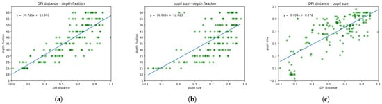
Figure 13.
Graphs for general normalized linear regression: (a) DPI distance vs. depth fixation, (b) pupil size vs. depth fixation, (c) DPI distance vs. pupil size, along with their corresponding graphs and equations (The darker areas of the points indicate regions where data points with the same value overlap, resulting in visually stronger colors).
The table below summarizes the R2 and RMSE results (Table 6).
Table 6.
R2 and RMSE for general normalized linear regression.
This resulted in R2 values of 0.69, 0.49, and 0.56, and RMSE values of 7.94, 10.25, and 0.18. For some subjects, these results were better than those from the models based on individual subject data.
4.4.2. Generalized Logistic Regression Analysis
The results of the logistic regression analysis based on data from all subjects are shown below (Figure 14).
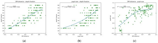
Figure 14.
Graphs for general logistic regression: (a) DPI distance vs. depth fixation, (b) pupil size vs. depth fixation, (c) DPI distance vs. pupil size, along with their corresponding graphs and equations (The darker areas of the points indicate regions where data points with the same value overlap, resulting in visually stronger colors).
The table below summarizes the R2 and RMSE results (Table 7).
Table 7.
R2 and RMSE for general logistic regression.
While the general logistic regression model did not match the best performance of the individual subject models, it did outperform the general linear regression model and some individual models.
4.4.3. Generalized Multiple Linear Regression Analysis
A multiple linear model was trained in order to define depth fixation as the relationship between DPI distance and pupil size. The graph below shows the results (Figure 15).
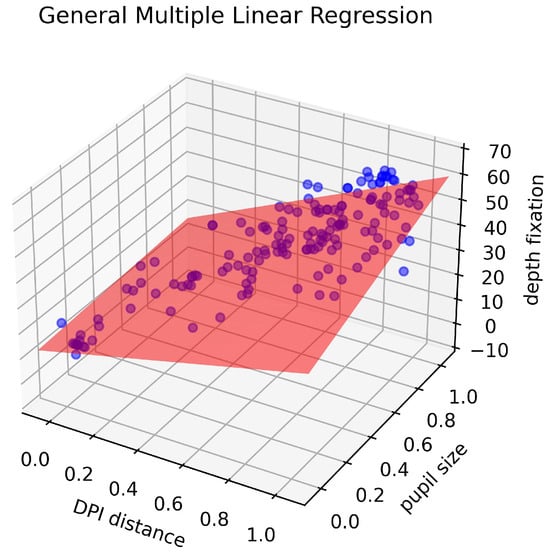
Figure 15.
Graphs for general multiple linear regression (The darker areas of the points indicate regions where data points with the same value overlap, resulting in visually stronger colors).
The R2, RMSE, and regression equations are provided below (Table 8).
Table 8.
R2, RMSE, and regression equations for general multiple linear regression.
As with the linear and logistic regression results, the general multiple linear model outperformed the individual models for some subjects. It also outperformed both the general linear model and the general logistic model. The regression equation derived from the general multiple linear model represents the relationship among depth fixation, DPI distance, and pupil size. This can be expressed as Equation (2).
5. Discussions
We additionally compared the performance of our model with existing binocular methods. We selected two binocular methods for comparison: an EOG-based method and a gaze vector-based method [9,10]. We used our general multiple linear regression model for the comparison, as it demonstrated the best performance among the general models.
Performance Comparison
The gaze vector-based study in [10] reported an average error distance of 0.42 ± 0.23 m and an average classification error rate of 9.92 ± 10.55%, with gaze depths ranging from 1 to 5 m at 1 m intervals. The EOG-based method in [9] achieved an average fixation distance error of 13.40 ± 11.80% (7.50 ± 5.60 cm) for the linear model and 10.30 ± 10.00% (5.70 ± 4.70 cm) for the neural network model over a range of distances from 20 to 90 cm. For performance comparison, the gaze vector-based method achieved 14.00% calculated using Equation (3). In this study, the RMSE was 7.69 cm, which corresponds to 20.51% according to Equation (3). The result calculated using Equation (4) was 15.36 ± 14.05%. A comparison of these results shows that although it does not match the performance of binocular-based estimation, it is still possible to estimate a meaningful level of gaze depth using a monocular method. Therefore, this method is worth considering as an alternative in scenarios where it is challenging to obtain binocular data or equipment.
6. Conclusions
This paper has examined changes in DPI distance and pupil size as a function of gaze depth and experimentally investigated their relationships. To do this, we captured right eye images from eleven subjects at ten different gaze depth levels. Purkinje images were generated using infrared LED, while eye videos were recorded with a single camera. We applied an algorithm based on contour and template matching to detect the pupil and DPI in the eye image, then calculated the pupil size and DPI distance. We conducted an analysis of data from eight subjects. For our analysis, the relationships between the variables were visualized using a scatter plot. In addition, a Spearman’s correlation analysis was performed. The results demonstrated that DPI distance vs. depth fixation, pupil size vs. depth fixation, and DPI distance vs. pupil size showed statistically significant positive correlations across all subjects. Our correlation and regression analyses revealed that stronger correlations do not necessarily correspond to better gaze depth prediction performance. In terms of RMSE and R2, DPI distance generally outperformed pupil size in estimating gaze depth. This is likely because pupil size is influenced by various factors other than gaze depth. For example, pupil size may not accurately reflect gaze depth because of psychological factors that are difficult to control during experiments. The multiple linear regression model provided more accurate predictions than the linear model and greater stability than the logistic model, indicating that incorporating two variables can provide enhanced performance compared to using a single variable. Finally, to formalize the relationship between the variables, we performed multiple linear regression using data from all subjects. This resulted in the following equation: depth fixation = 20.746·DPI distance + 5.223·pupil size + 16.495·DPI distance·pupil size + 13.880, which achieved an R2 of 0.71 and RMSE of 7.69. This result represents the best performance of the general models, indicating that it can make reasonably accurate predictions, although it does not outperform the binocular based method. These results support the hypothesis that gaze depth can be estimated from DPI distance, and demonstrates their close relationship.
Limitations and Future Work
This experiment used the length of the detected ellipse obtained through an ellipse estimation algorithm as the measure of pupil size. This value differs from the actual pupil size, which may affect the results of our analysis. To enhance prediction performance, the measurement method should be improved in future research. Second, our experiment acquired the right eye images from all subjects. However, individuals may have different dominant eyes, which should be taken into account in future research to improve the results. Third, Purkinje images were not captured for some subjects, and sometimes could not be detected even within the same subject due to changes in eye features depending on the gaze depth. To improve data collection, the camera position and LED conditions should be adjusted in order to ensure consistency across all subjects. Fourth, we sought to minimize the influence of external factors in this experiment by limiting the subject’s movement and using a constant image as input. This approach is generally applicable to traditional VR/AR environments where the eye tracker is fixed to the HMD. However, it becomes difficult to apply this method in environments where the relative position of the camera and the eye is constantly changing. Fifth, the experiment had a small number of subjects and did not account for physiological differences. In myopic subjects, the eye has reduced ability to adjust the thickness of the lens, which affects the DPI distance. These differences must be considered in order for the results to be universally applicable. Because they were not accounted for in this study, the results are more difficult to generalize, and the defined relationships may not be statistically significant.
Although the experimental results are difficult to generalize due to the lack of consideration of physiological differences, this also means that the results reflect the unique physiological characteristics of each subject. This finding can be used to provide personalized services. In future work, we plan to offer a personalized service that estimates gaze depth using only DPI distance and pupil size through initial calibration. This service could be applied to 3D applications and implemented in fields such as gaming, shopping, marketing, and more. We also aim to explore the applicability of this experiment in mild non-controlled environments. For example, we plan to investigate whether DPI distance and pupil size can still be detected under image transformations such as scaling and rotation, as well as to consider the use of motion compensation techniques. We intend to recruit a larger number of subjects in order to account for different age groups and physiological conditions. If we can define a generalized expression for a wide range of subjects, it could serve as a diagnostic indicator of abnormalities in lens thickness or pupil size control. For instance, a significant difference between the derived and actual measured values might indicate an abnormality in these control functions. Moreover, comparing results across different age groups and physiological conditions could enhance the quality of personalized services.
Author Contributions
Conceptualization, E.C.L.; methodology, E.C.L. and J.A.; software, J.A.; validation, J.A.; formal analysis, J.A.; investigation, J.A.; resources, E.C.L. and J.A.; data curation, J.A.; writing—original draft preparation, J.A.; writing—review and editing, E.C.L.; supervision, E.C.L.; project administration, E.C.L. All authors have read and agreed to the published version of the manuscript.
Funding
This work was supported by the NRF (National Research Foundation) of Korea funded by the Korean government (Ministry of Science and ICT) (RS-2024-00340935).
Institutional Review Board Statement
This study was approved by the Sangmyung University Institutional Bioethics Review Board on 4 July 2024. (SMUIRB(S-2024-013)).
Informed Consent Statement
Informed consent was obtained from all subjects involved in the study.
Data Availability Statement
The data used in this article are available upon request due to restrictions.
Conflicts of Interest
The authors declare no conflicts of interest.
Abbreviations
The following abbreviations are used in this manuscript:
| DPI | Dual Purkinje Images |
| VR | Virtual Reality |
| AR | Augmented Reality |
| IPD | Interpupillary Distance |
| EVA | Eye Vergence Angle |
| EOG | Electrooculography |
| MLP | Multi-Layer Perceptron |
| VOR | Vestibulo-Ocular Reflex |
| ROI | Region of Interest |
| PROI | Purkinje Image Region of Interest |
| HMD | Head-Mounted Display |
References
- Yang, Q.; Wang, T.; Su, N.; Xiao, S.; Kapoula, Z. Specific saccade deficits in patients with Alzheimer’s disease at mild to moderate stage and in patients with amnestic mild cognitive impairment. Age 2013, 35, 1287–1298. [Google Scholar] [CrossRef] [PubMed]
- Raney, G.E.; Campbell, S.J.; Bovee, J.C. Using eye movements to evaluate the cognitive processes involved in text comprehension. J. Vis. Exp. 2014, 83, 50780. [Google Scholar] [CrossRef] [PubMed]
- Hammer, J.H.; Maurus, M.; Beyerer, J. Real-time 3D gaze analysis in mobile applications. In Proceedings of the 2013 Conference on Eye Tracking South Africa, Cape Town, South Africa, 29–31 August 2013; pp. 75–78. [Google Scholar] [CrossRef]
- Alt, F.; Schneegass, S.; Auda, J.; Rzayev, R.; Broy, N. Using eye-tracking to support interaction with layered 3D interfaces on stereoscopic displays. In Proceedings of the 19th International Conference on Intelligent User Interfaces, Haifa, Israel, 24–27 February 2014; pp. 267–272. [Google Scholar] [CrossRef]
- Lee, E.C.; Ko, Y.J.; Park, K.R. Fake iris detection method using Purkinje images based on gaze position. Opt. Eng. 2008, 47, 067204. [Google Scholar] [CrossRef]
- Arefin, M.S.; Swan, J.E., II; Cohen Hoffing, R.A.; Thurman, S.M. Estimating perceptual depth changes with eye vergence and interpupillary distance using an eye tracker in virtual reality. In Proceedings of the 2022 Symposium on Eye Tracking Research and Applications, Seattle, WA, USA, 8–11 June 2022; pp. 1–7. [Google Scholar] [CrossRef]
- Iskander, J.; Hossny, M.; Nahavandi, S. Using biomechanics to investigate the effect of VR on eye vergence system. Appl. Ergon. 2019, 81, 102883. [Google Scholar] [CrossRef] [PubMed]
- Dodgson, N.A. Variation and extrema of human interpupillary distance. Stereosc. Displays Virtual Real. Syst. XI 2004, 5291, 36–46. [Google Scholar] [CrossRef]
- Stevenson, C.; Jung, T.P.; Cauwenberghs, G. Estimating direction and depth of visual fixation using electrooculography. In Proceedings of the 2015 37th Annual International Conference of the IEEE Engineering in Medicine and Biology Society (EMBC), Milan, Italy, 25–29 August 2015; IEEE: Piscataway, NJ, USA, 2015; pp. 841–844. [Google Scholar] [CrossRef] [PubMed]
- Lee, Y.; Shin, C.; Plopski, A.; Itoh, Y.; Piumsomboon, T.; Dey, A.; Lee, G.; Kim, S.; Billinghurst, M. Estimating gaze depth using multi-layer perceptron. In Proceedings of the 2017 International Symposium on Ubiquitous Virtual Reality (ISUVR), Nara, Japan, 28–30 June 2017; IEEE: Piscataway, NJ, USA, 2017; pp. 26–29. [Google Scholar] [CrossRef]
- Kassner, M.; Patera, W.; Bulling, A. Pupil: An open source platform for pervasive eye tracking and mobile gaze-based interaction. In Proceedings of the 2014 ACM International Joint Conference on Pervasive and Ubiquitous Computing: Adjunct Publication, Seattle, WA, USA, 13–17 September 2014; pp. 1151–1160. [Google Scholar] [CrossRef]
- Zhang, C.; Chen, T.; Shaffer, E.; Soltanaghai, E. FocusFlow: 3D Gaze-Depth Interaction in Virtual Reality Leveraging Active Visual Depth Manipulation. In Proceedings of the 2024 CHI Conference on Human Factors in Computing Systems, Honolulu, HI, USA, 11–16 May 2024; pp. 1–18. [Google Scholar] [CrossRef]
- Li, C.; Tong, E.; Zhang, K.; Cheng, N.; Lai, Z.; Pan, Z. Gaze Estimation Based on a Multi-Stream Adaptive Feature Fusion Network. Appl. Sci. 2025, 15, 3684. [Google Scholar] [CrossRef]
- Mardanbegi, D.; Clarke, C.; Gellersen, H. Monocular gaze depth estimation using the vestibulo-ocular reflex. In Proceedings of the 11th ACM Symposium on Eye Tracking Research & Applications, Denver, CO, USA, 25–28 June 2019; pp. 1–9. [Google Scholar] [CrossRef]
- Mansouryar, M.; Steil, J.; Sugano, Y.; Bulling, A. 3D gaze estimation from 2D pupil positions on monocular head-mounted eye trackers. In Proceedings of the Ninth Biennial ACM Symposium on Eye Tracking Research & Applications, Charleston, SC, USA, 14–17 March 2016; pp. 197–200. [Google Scholar] [CrossRef]
- Wang, X.; Lindlbauer, D.; Lessig, C.; Alexa, M. Accuracy of monocular gaze tracking on 3d geometry. In Proceedings of the Eye Tracking and Visualization: Foundations, Techniques, and Applications, ETVIS 2015, Chicago, IL, USA, 25 October 2015; Springer: Cham, Switzerland, 2017; pp. 169–184. [Google Scholar] [CrossRef]
- Lee, J.W.; Cho, C.W.; Shin, K.Y.; Lee, E.C.; Park, K.R. 3D gaze tracking method using Purkinje images on eye optical model and pupil. Opt. Lasers Eng. 2012, 50, 736–751. [Google Scholar] [CrossRef]
- Lee, E.C.; Lee, J.W.; Park, K.R. Experimental investigations of pupil accommodation factors. Investig. Ophthalmol. Vis. Sci. 2011, 52, 6478–6485. [Google Scholar] [CrossRef] [PubMed]
- Lee, C.L.; Pei, W.; Lin, Y.C.; Granmo, A.; Liu, K.H. Emotion detection based on pupil variation. Healthcare 2023, 11, 322. [Google Scholar] [CrossRef] [PubMed]
- Park, S.; Park, Y.J.; Lee, M.; Lee, E.C. Study on the Measurement of Visual Fatigue in Welding Mask Wearers through Infrared Eye Image Features. J. Next-Gener. Converg. Technol. Assoc. 2024, 8, 245–254. [Google Scholar] [CrossRef]
- Wu, R.J.; Clark, A.M.; Cox, M.A.; Intoy, J.; Jolly, P.C.; Zhao, Z.; Rucci, M. High-resolution eye-tracking via digital imaging of Purkinje reflections. J. Vis. 2023, 23, 4. [Google Scholar] [CrossRef] [PubMed]
- Lu, C.; Chakravarthula, P.; Tao, Y.; Chen, S.; Fuchs, H. Improved vergence and accommodation via purkinje image tracking with multiple cameras for ar glasses. In Proceedings of the 2020 IEEE International Symposium on Mixed and Augmented Reality (ISMAR), Porto de Galinhas, Brazil, 9–13 November 2020; IEEE: Piscataway, NJ, USA, 2020; pp. 320–331. [Google Scholar] [CrossRef]
Disclaimer/Publisher’s Note: The statements, opinions and data contained in all publications are solely those of the individual author(s) and contributor(s) and not of MDPI and/or the editor(s). MDPI and/or the editor(s) disclaim responsibility for any injury to people or property resulting from any ideas, methods, instructions or products referred to in the content. |
© 2025 by the authors. Licensee MDPI, Basel, Switzerland. This article is an open access article distributed under the terms and conditions of the Creative Commons Attribution (CC BY) license (https://creativecommons.org/licenses/by/4.0/).