

Modular Multilevel Converter Control Strategy for AC Fault Current Maximization and Grid Code Compliance


Abstract
1. Introduction
2. Grid Codes
- Capability of staying connected to the network within given ranges of the network voltage.
- Capability to provide fast fault current injection at the connection point in case of a symmetrical fault (in coordination with the relevant TSO).
- Asymmetrical current injection in case of an asymmetrical fault (in coordination with the relevant TSO).
- Fault-ride-through capability.
- Power park modules must be capable of managing the rapid injection of fault current through a continuous control system.
- They shall have the capability to inject apparent current per phase that is at least equal to their nominal current.
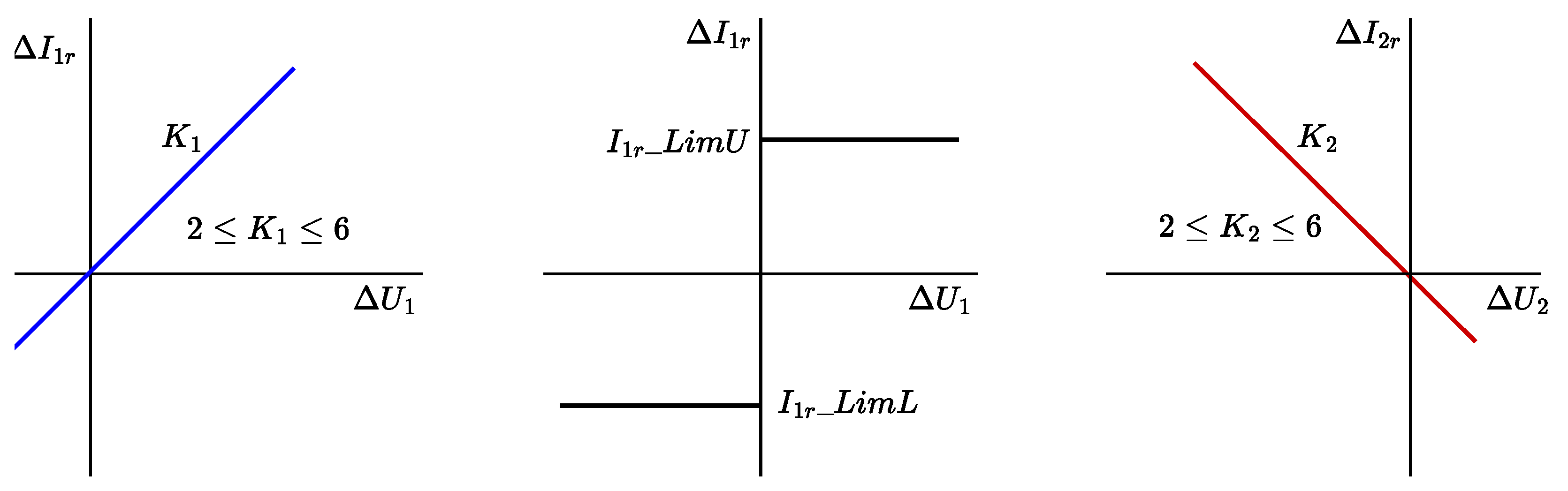
- For the positive-sequence current, power park modules must inject or absorb, depending on the positive-sequence voltage error , a reactive current (pu) through a continuous proportional control (see Figure 1). The default value for the limit of this current is pu.
- In addition to the total reactive current component , power park modules must inject an active current component.
- For the negative sequence current, power park modules must inject or absorb, depending on the negative sequence voltage error , a negative sequence current through a continuous proportional control (see Figure 1).
- For balanced faults, IBR units shall inject reactive current dependent on the terminal voltage of the IBR unit. The difference between the reactive current during a fault and the pre-fault reactive current is the incremental positive-sequence reactive current . During a fault condition, priority shall be given to reactive current injection with any residual capacity being supplied as active current unless the IBR unit is specified to operate in active current priority mode by the TSO.
- For unbalanced faults, in addition to increasing positive-sequence reactive current, the IBR unit shall inject negative-sequence current , dependent on IBR unit terminal negative-sequence voltage. If the IBR unit’s total current limit is reached, either or , or both may be reduced with a preference of equal reduction in both currents.
- This standard intentionally does not specify magnitude of incremental positive- and negative-sequence reactive current injection during a fault condition. The TSO should consider specifying the required magnitudes.
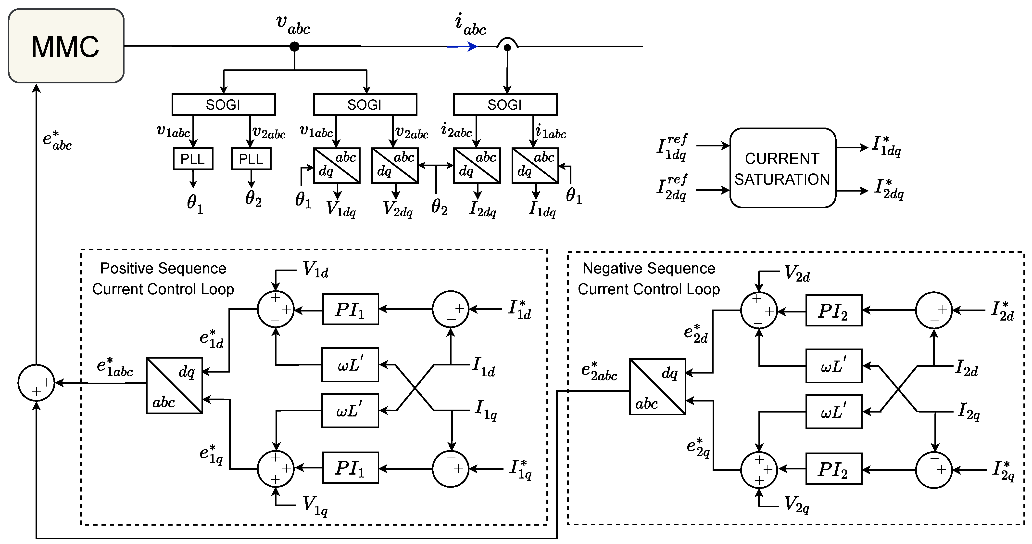
3. System and Control Description
4. Current Saturation Strategies
4.1. Output Current Saturation with Fixed Limits: Saturation Algorithm 1 (sat1)
4.2. Output Current Saturation with Dynamic Limits: Saturation Algorithm 2 (sat2)
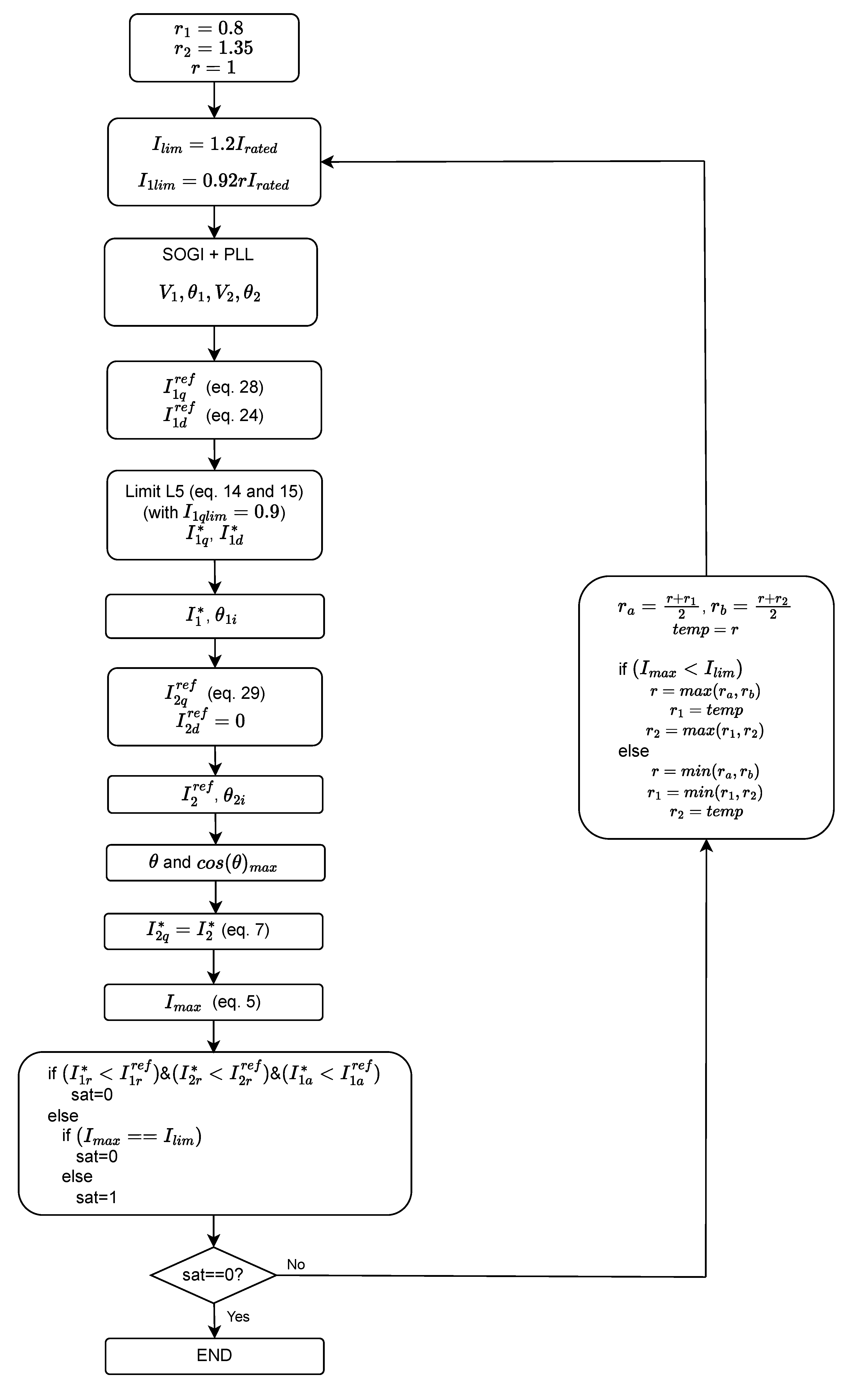
- Step 1: Define the limits of the output current () and the positive-sequence current (). In the figure, these limits are set to pu (assuming a 20% overload capability) and pu (with ), but other values could be used. To maximize the injected current, the positive sequence current limit is adjusted through an iterative process that modifies the variable r. Initially, this variable is set to 1. For subsequent iterations, an updated value of r is computed using its value in the two previous iterations, which are denoted as and , respectively. Since there are no prior values of r for the second iteration, the initial values of 0.8 and 1.35 are assigned to and , respectively.
- Step 2: Compute the positive- and negative-sequence voltages ( and ) and their angles ( and ) from the grid measurements by using the SOGI and the PLL (see Figure 3).
- Step 4: Obtain the saturated current references and of the positive-sequence according to Equations (15) and (14), respectively. Note that the injection of the reactive current is prioritized. The limit is set at 0.9 according to the Spanish Grid Code.
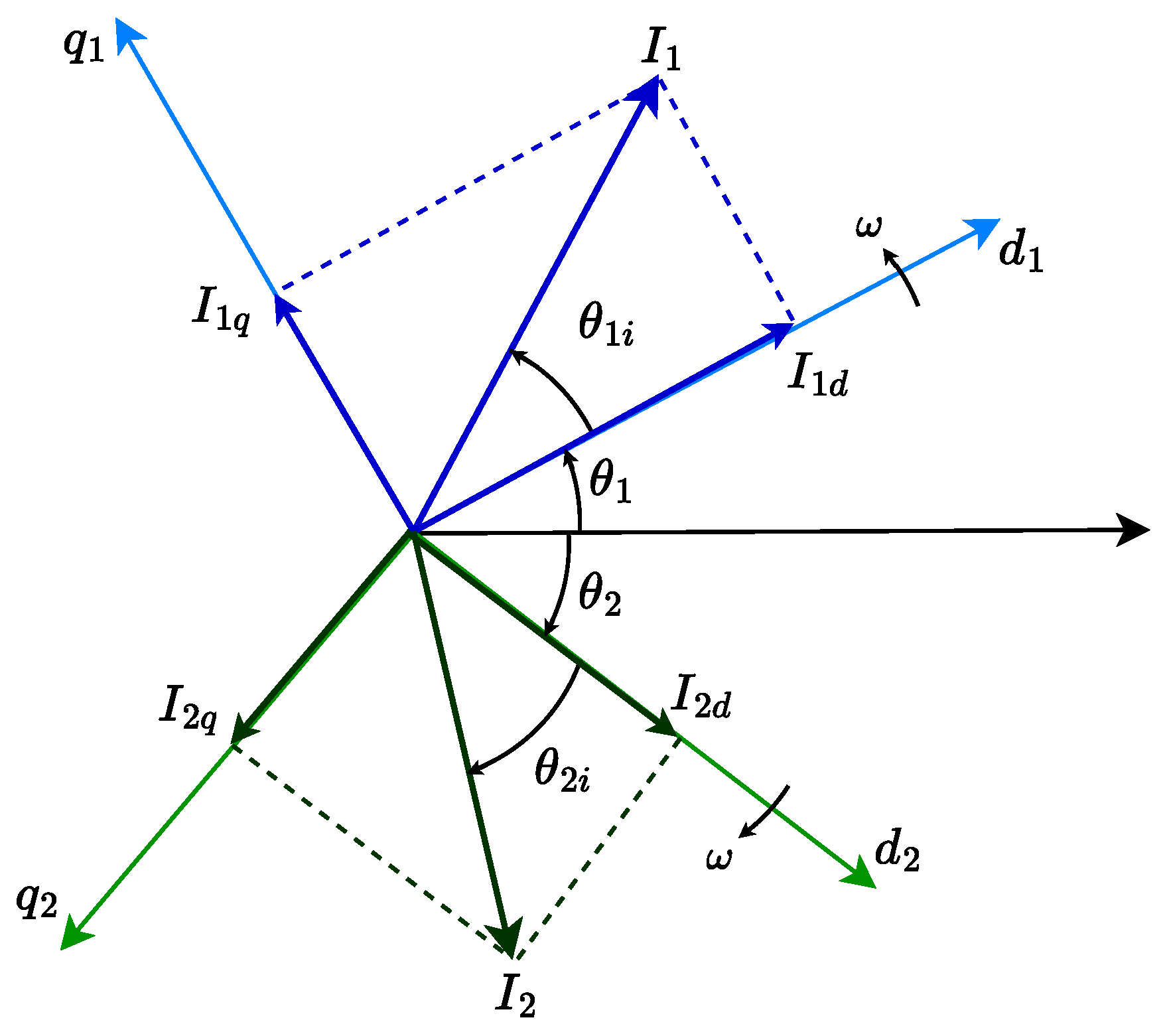
- Step 5: Compute the magnitude () and the angle () of the saturated positive-sequence current.
- Step 6: Compute the non-saturated reference of the negative-sequence reactive current () according to the grid code (Equation (29)).
- Step 7: Compute the magnitude () and the angle () of the negative-sequence current.
- Step 8: Compute to determine the phase with the highest current. Note that it is necessary to know the angles , , and . The first three angles were already calculated in steps 2 and 5. depends on the values of the active and reactive currents. However, given that the negative-sequence active current is always set to zero, is always , regardless of the saturation.
- Step 9: The maximum negative-sequence current is calculated using and the output current limit according to Equation (5). Using Equation (7), the saturated negative-sequence current reference () is calculated (note that given that ).
- Step 10: Using the saturated currents and , and , the output current of the phase with the highest value is computed using Equation (5).
- Step 11: Four cases may occur:
- −
- and : None of the currents saturate; hence, the MMC tracks its current references and the loop ends.
- −
- and : Both currents are saturated; hence, the MMC injects its maximum current according to the grid code. The loop ends.
- −
- and : The positive-sequence current reaches its limit but the output current does not (for instance, for a three-phase short-circuit that does not require injecting negative-sequence current). In this case, the loop returns to the first step and increases the limit of the positive-sequence current. This is achieved by means of the variable r, which is modified in each iteration to search for the current limits.
- −
- and : The MMC tracks the positive-current reference because is not saturated. The remaining margin is assigned to the negative-sequence current up to the output current limit. The loop ends because the output current reaches its limit.
4.3. Arm Current Saturation with Dynamic Limits: Saturation Algorithm 3 (sat3)
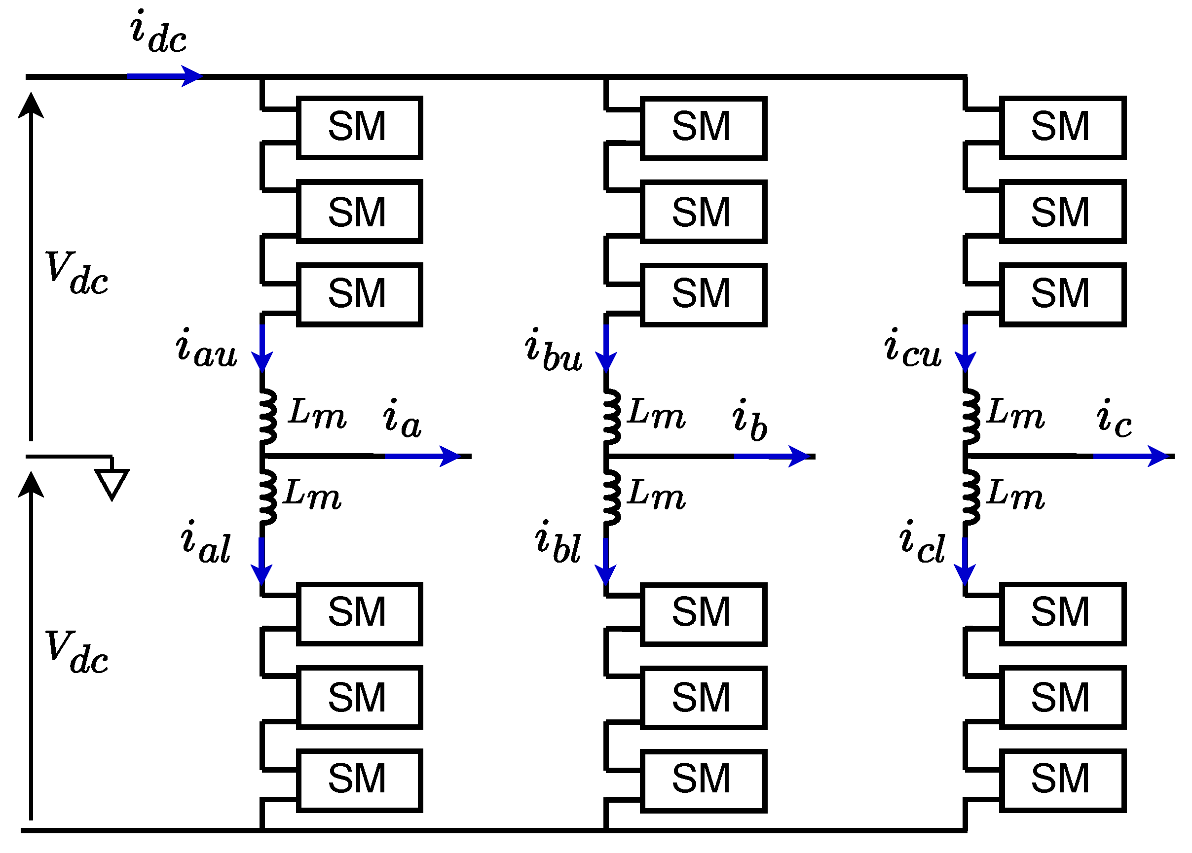
- Step 11: Using the phase with the highest output current and the DC current, the arm with the highest current is computed (Equation (34)). Note that the grid voltage , obtained in step 2, the output current , and the DC current , calculated in step 10, are used instead of the rated values in Equation (34).
- Step 12: Three cases may occur:
- −
- and and : Since none of the currents reach saturation, the MMC is able to track the current references, and the control loop terminates.
- −
- or : The positive-sequence current saturates.
- ∘
- : The arm current does not saturate; hence, the negative-sequence component does not saturate either. Therefore, there is still some margin to increase the positive-sequence current. In this case, the loop returns to the initial step and increases both the output current limit and the positive-sequence current limit. This is achieved through the variable r, which is modified in each iteration to search for the current limits.
- ∘
- : The arm current saturates and the loop ends.
5. Results
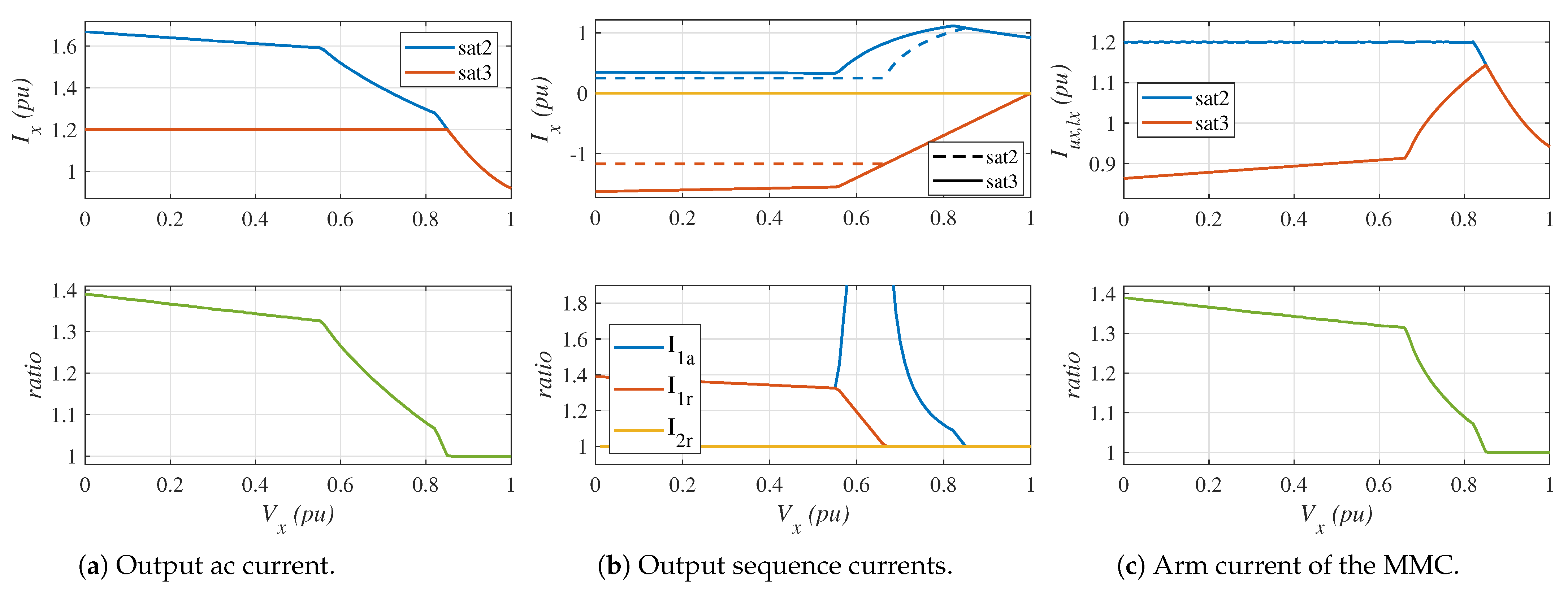
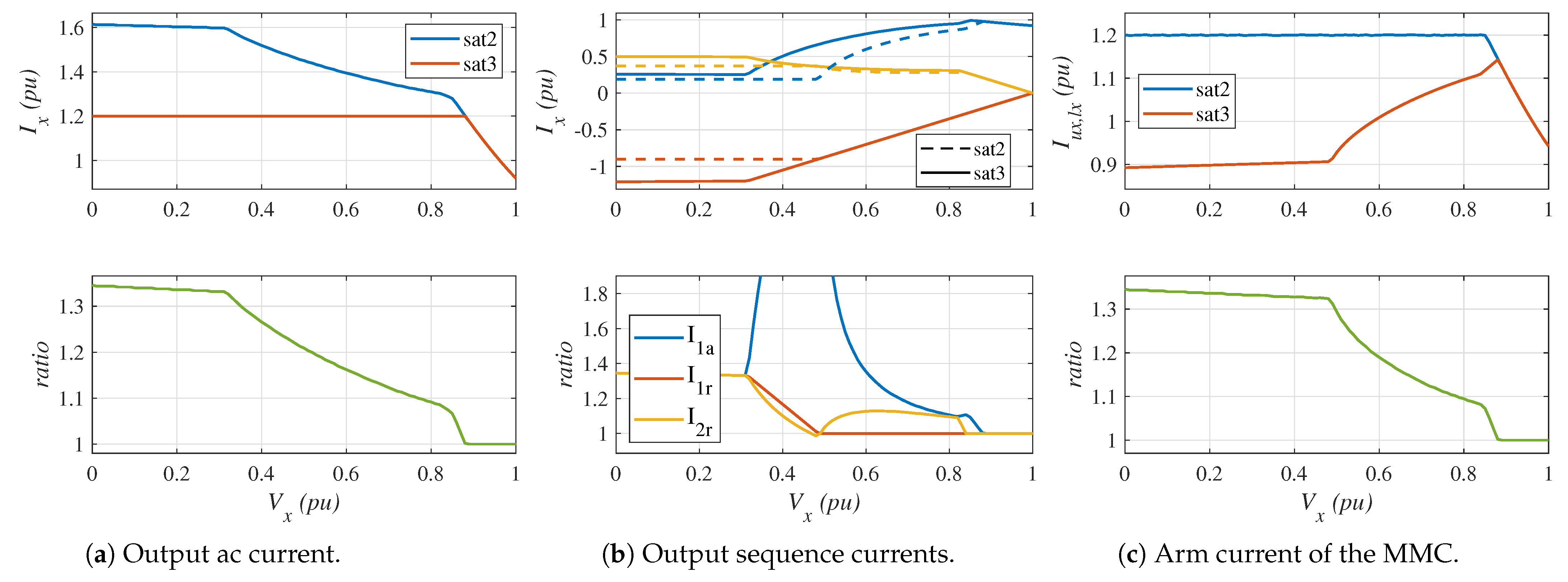
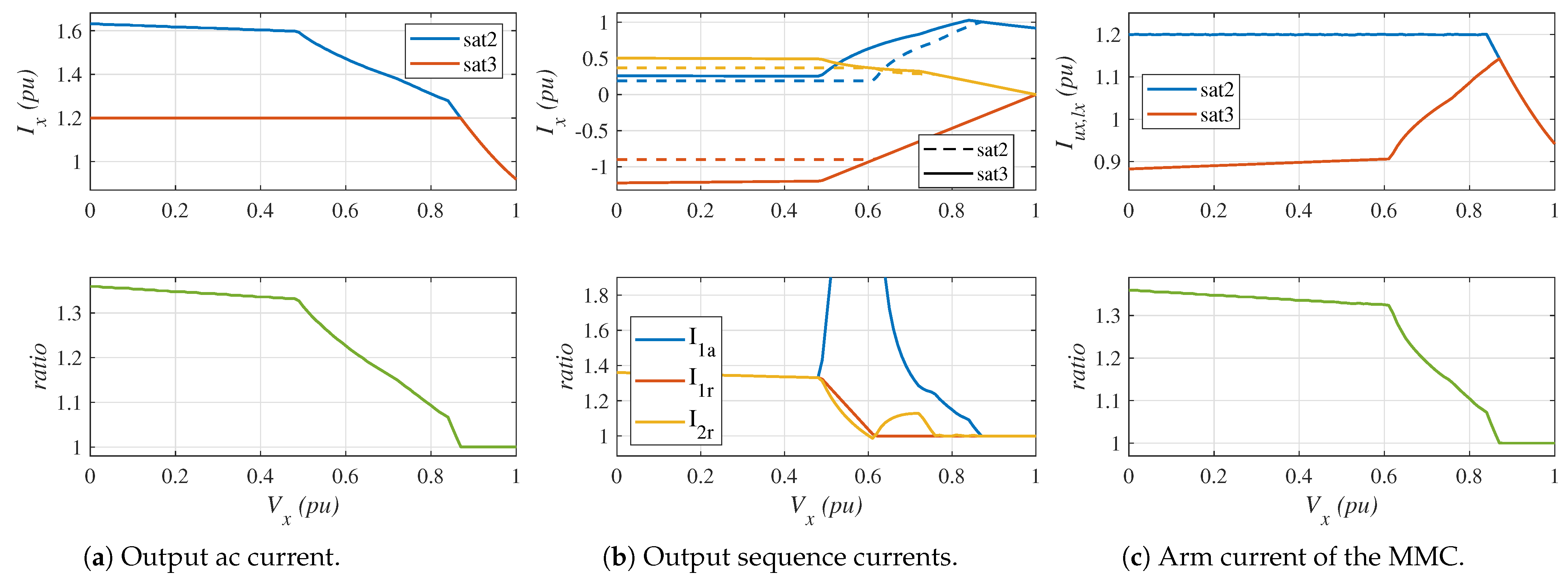
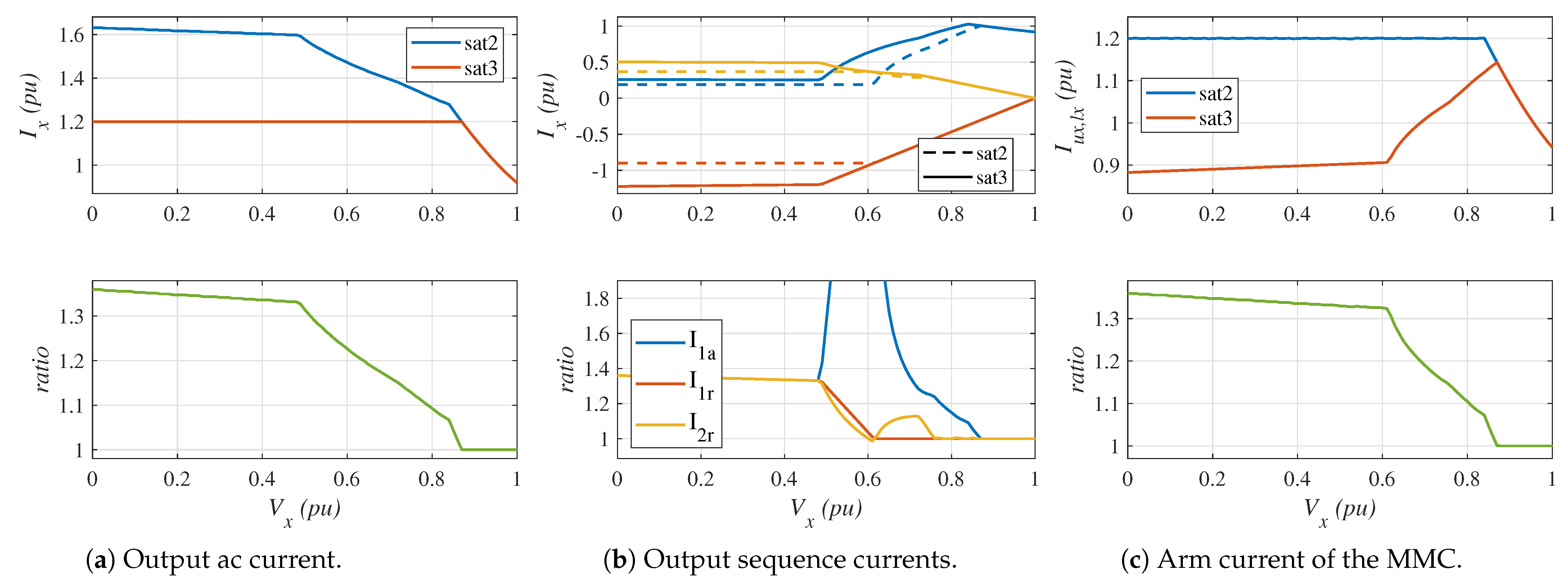
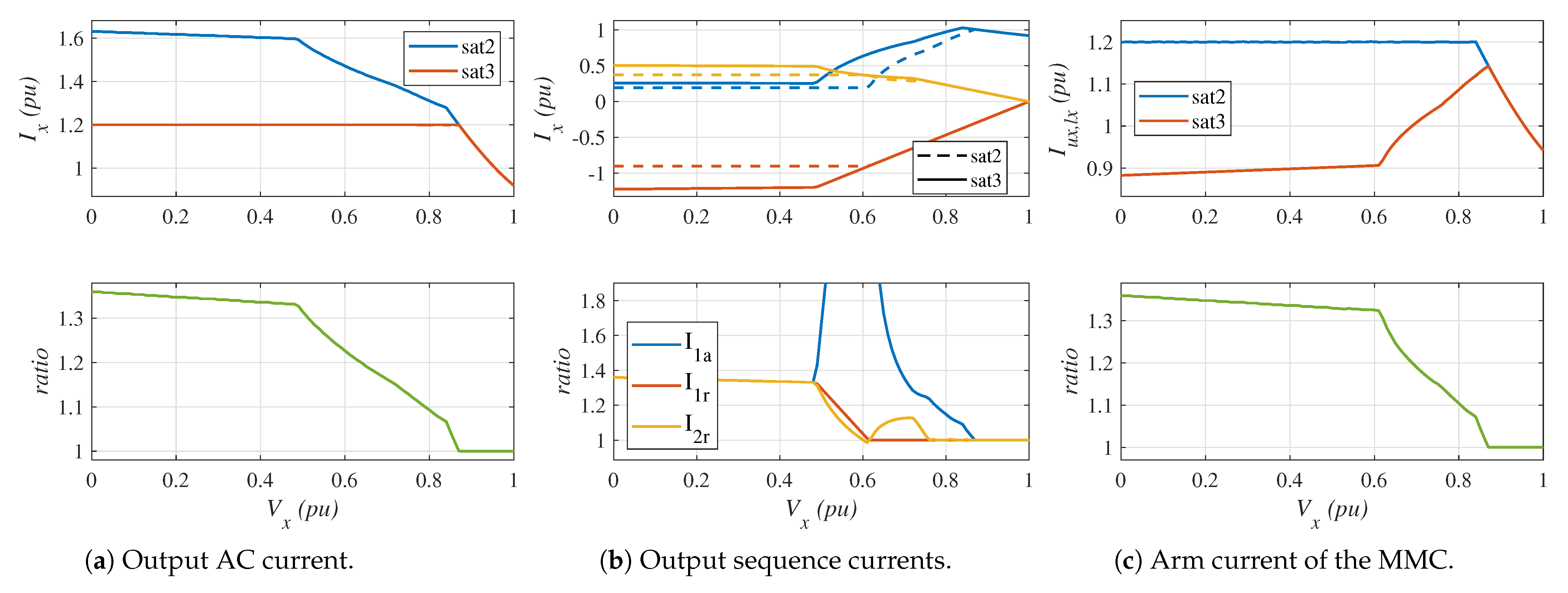
- Top-left graph: It shows the output AC current considering the saturation algorithms described in Section 4.2 (red line) and Section 4.3 (blue line). In both cases, the phase with the highest current is plotted.
- Bottom-left graph: The ratio of the output current with saturation strategy 3 to the output current with saturation strategy 2 is plotted.
- Top-center graph: It shows the output positive-sequence reactive current (), the positive-sequence active current (), and the negative-sequence reactive current (). Again, the saturation algorithm described in Section 4.2 (dashed lines) is compared with the saturation algorithm described in Section 4.3 (solid lines). In both cases, the phase with the highest current is plotted.
- Bottom-center graph: The ratio of the sequence currents with saturation strategy 3 to the sequence currents with saturation strategy 2 is plotted.
- Top-right graph: It shows the peak arm current of the MMC considering the saturation algorithms presented in Section 4.2 (red line) and that in Section 4.3 (blue line). In both cases, the arm with the highest current is plotted.
- Bottom-left graph: The ratio of the arm current with saturation strategy 3 to the arm current with saturation strategy 2 is plotted.
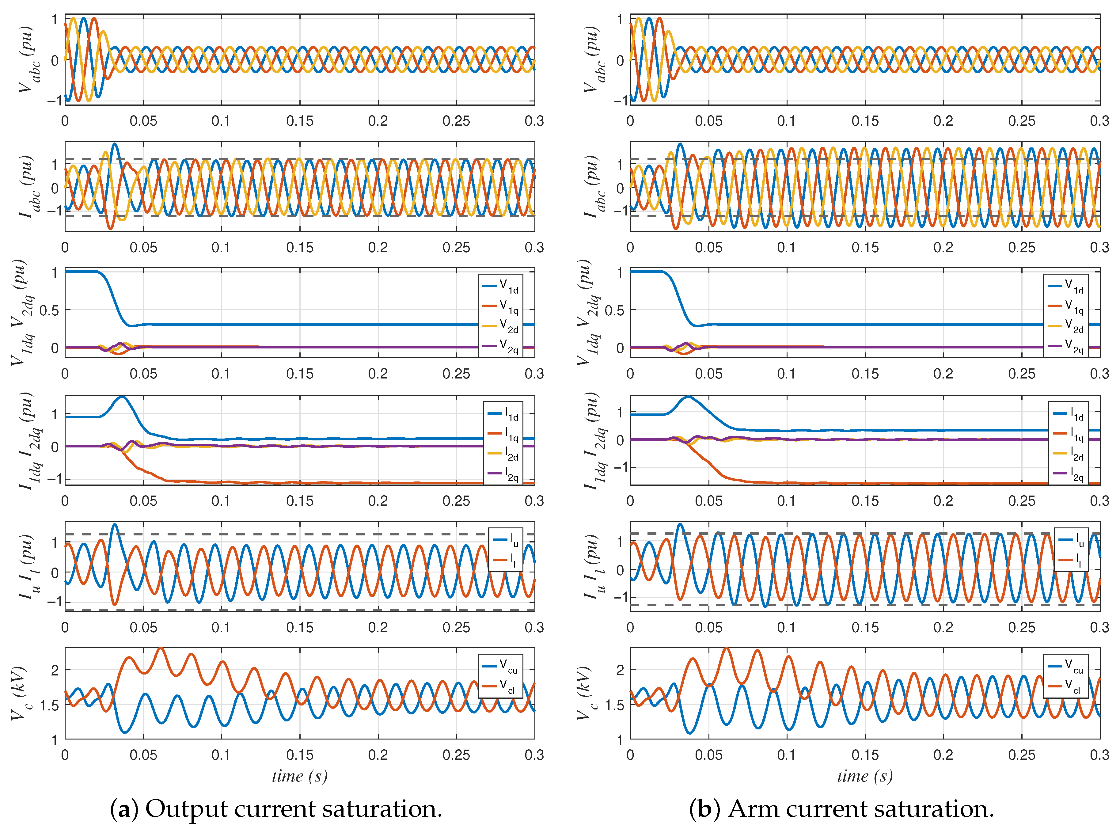
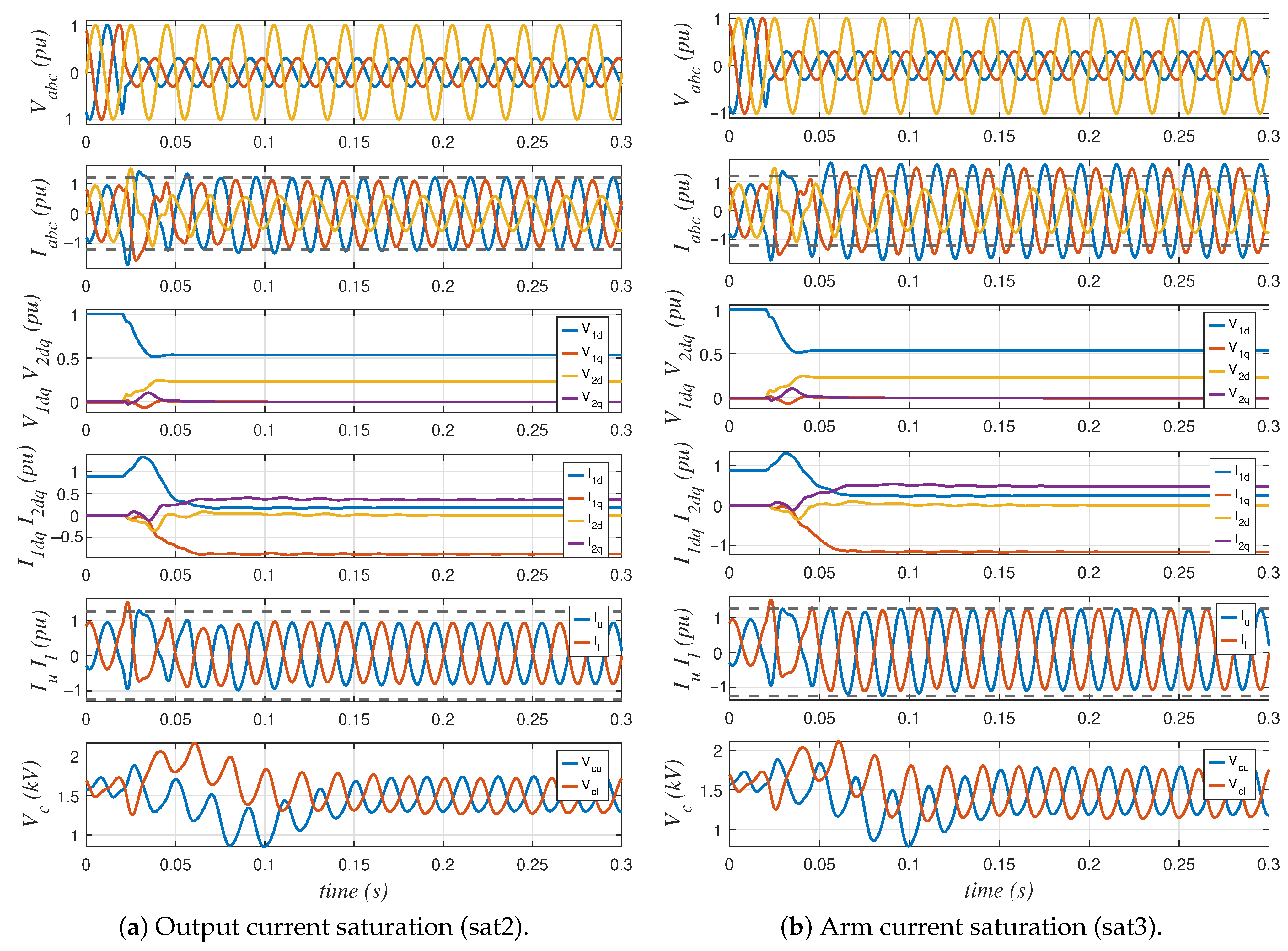
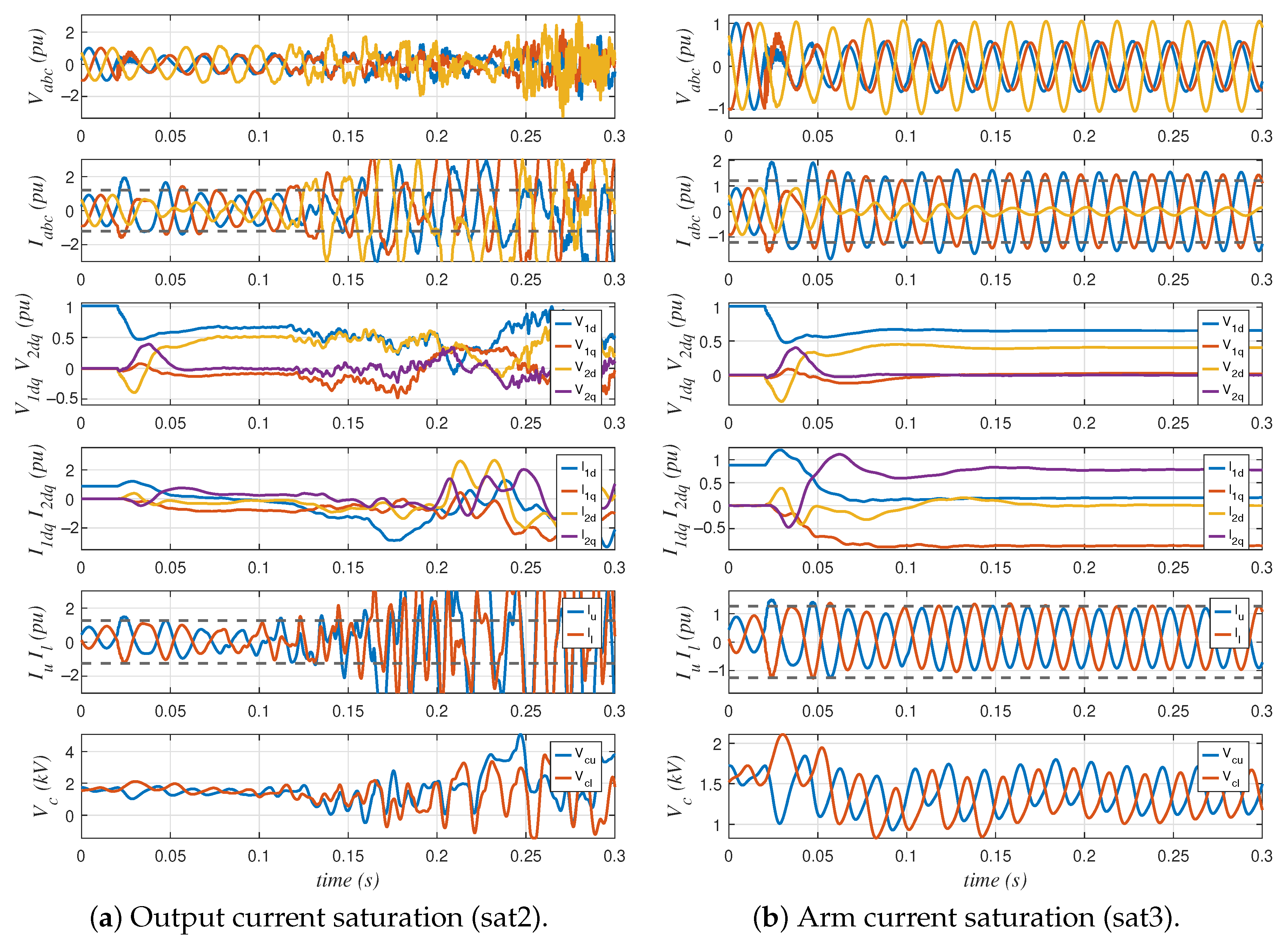
Simulation Results
6. Conclusions
Author Contributions
Funding
Data Availability Statement
Conflicts of Interest
Abbreviations
| GC | Grid Code |
| HVDC | High-Voltage Direct Current |
| MMC | Modular Multilevel Converter |
| PEC | Power Electronic Converter |
| PLL | Phase-Locked Loop |
| SC | Synchronous Condenser |
| SCL | Short-Circuit Level |
| SG | Synchronous Generator |
| SOGI | Second Order Generalized Integrator |
| TSO | Transmission System Operator |
| VSC | Voltage Source Converter |
Appendix A
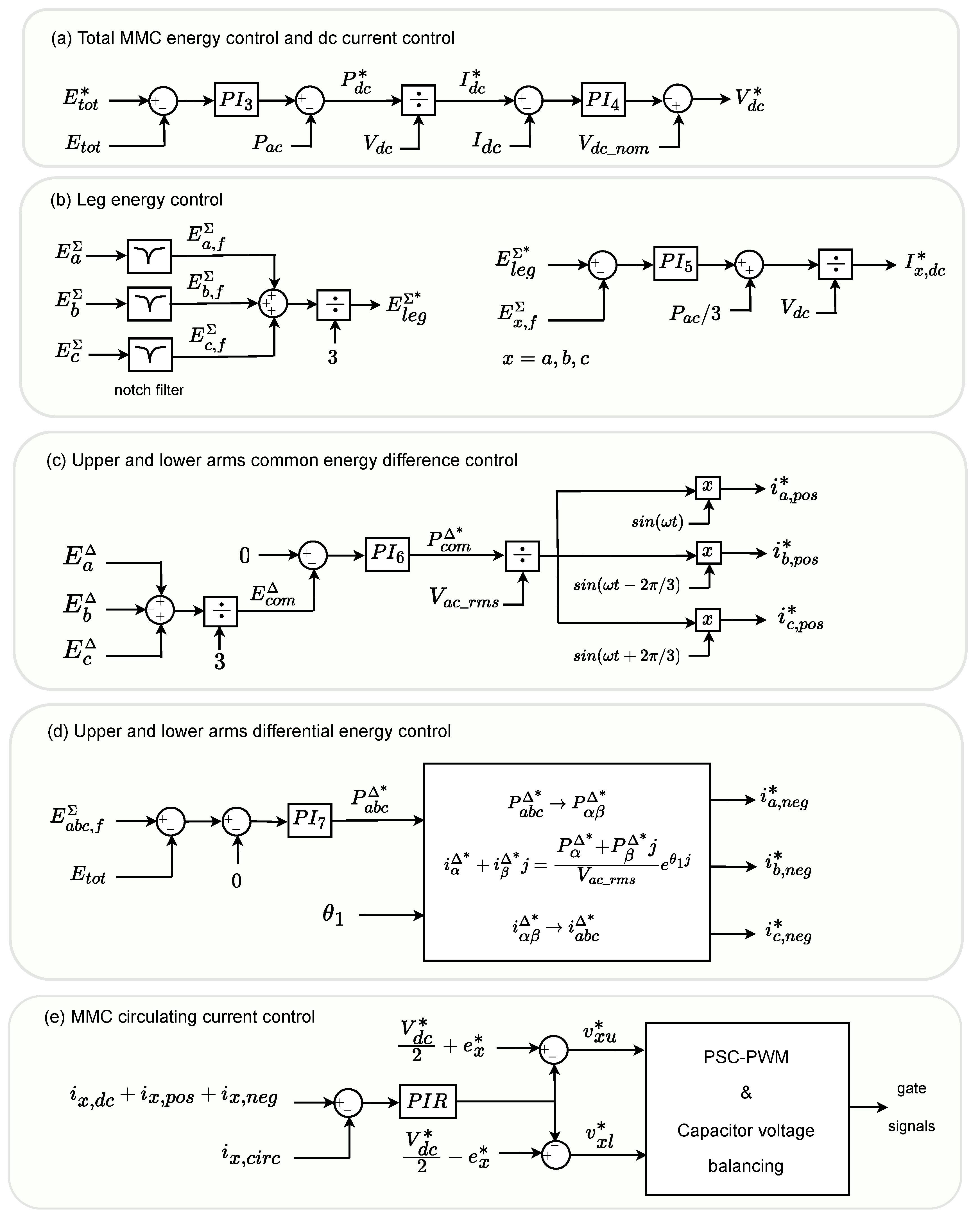
Appendix A.1. Inner Control of the MMC
Appendix A.2. Control Parameters

| Controllers/Filters | Values |
|---|---|
| 1: positive sequence output current control | V/A, V/As |
| : negative sequence output current control | V/A, V/As |
| : total MMC energy control | W/J, W/Js |
| : dc current control | V/A, V/As |
| : leg energy control | W/J, W/Js |
| : upper and lower arms common energy difference control | W/J, W/Js |
| : upper and lower arms differential energy control | W/J, W/Js |
| 2: MMC circulating current control | V/A, V/As |
| V/A, rad/s | |
| Band reject filter 3 | Vs2/A, Vs/A |
| V/A, s2 | |
| s, |
Appendix B


References
- IEEE Power & Energy Society. Impact of Inverter Based Generation on Bulk Power System Dynamics and Short-Circuit Performance. Technical Report. 2018. Available online: https://resourcecenter.ieee.org/publications/technical-reports/pes_tr_7-18_0068 (accessed on 14 March 2025).
- National Grid ESO. System Operability Framework Lmpact of Declining Short Circuit Levels; Technical Report; National Grid ESO: Warwick, UK, 2018. [Google Scholar]
- Belenguer, E.; Vidal-Albalate, R.; Magraner, F. Fault analysis of power systems dominated by Power Electronic Interfaced Devices. In Proceedings of the ELECTRIMACS 2024—International Conference on Modeling and Simulation of Electric Machines, Converters and Systems, Castelló, Spain, 27–30 May 2024. [Google Scholar]
- National Grid ESO. System Operability Framework Whole System Short Circuit Levels; Technical Report; National Grid ESO: Warwick, UK, 2018. [Google Scholar]
- Aljarrah, R.; Marzooghi, H.; Terzija, V. Mitigating the impact of fault level shortfall in future power systems with high penetration of converter-interfaced renewable energy sources. Int. J. Electr. Power Energy Syst. 2023, 149, 109058. [Google Scholar] [CrossRef]
- Weise, B. Impact of K-factor and active current reduction during fault-ride-through of generating units connected via voltage-sourced converters on power system stability. IET Renew. Power Gener. 2015, 9, 25–36. [Google Scholar] [CrossRef]
- Wang, S.; Egea-Alvarez, A. Operating a Zero Carbon GB Power System in 2025: Frequency and Fault Current. Power Electronic Devices and Fault Current. Technical Report. 2020. Available online: https://strathprints.strath.ac.uk/74793/ (accessed on 14 March 2025).
- Nedd, M.; Hong, Q.; Bell, K.; Booth, C.; Mohapatra, P. Application of Synchronous Compensators in the GB Transmission Network to Address Protection Challenges from Increasing Renewable Generation. In Proceedings of the CIGRE (Study Committee B5 Colloquium), Auckland, New Zealand, 11–15 September 2017. [Google Scholar]
- Gordon, S.; Hong, Q.; Bell, K. Implications of reduced fault level and its relationship to system strength: A Scotland case study. In Proceedings of the CIGRE, Paris, France, 28 August–2 September 2022. [Google Scholar]
- National Grid ESO. NOA Stability Pathfinder Phase 2. Expression of Interest Summary. Available online: https://www.neso.energy/document/187371/download (accessed on 18 February 2025).
- pse2consulting. The National Grid Pathfinder 2 Project. Available online: https://pse2consulting.com/national-grid-pathfinder (accessed on 18 February 2025).
- Elecnor. Elecnor to Participate in the NOA Stability Pathfinder Programme in Scotland. Available online: https://www.grupoelecnor.com/storage/media/files/shares/noticias/en/elecnorukwpthurso-and-neilstonnpen.pdf (accessed on 18 February 2025).
- ABB. ABB’s Integrated Technology Will Stabilize the Power Grid as Spanish Islands Transition to Green Energy. Available online: https://new.abb.com/news/detail/116318/abbs-integrated-technology-will-stabilize-the-power-grid-as-spanish-islands-transition-to-green-energy (accessed on 18 February 2025).
- Vidal-Albalate, R.; Belenguer, E.; Magraner, F.; El Ghoufairi, Y. Influence of converter control on directional and fault identification algorithms of protective relays. In Proceedings of the 2024 ONCON—The 3rd IEEE Industrial Electronics Society Annual Online Conference, Beijing, China, 8–10 December 2024. [Google Scholar]
- Ministry for the Ecological Transition and the Demographic Challenge. Orden TED/749/2020, de 16 de Julio, por la que se Establecen los Requisitos téCnicos Para la Conexión a la Red Necesarios Para la Implementación de los Códigos de Red de Conexión (Technical Requirements for Grid Connection Necessary for the Implementation of the Network Connection Codes). Available online: https://www.boe.es/buscar/act.php?id=BOE-A-2020-8965 (accessed on 15 February 2025).
- Technical Connection Rules for High-Voltage (VDE-AR-N 4120). Available online: https://www.vde.com/en/fnn/topics/technical-connection-rules/tar-for-high-voltage (accessed on 25 February 2025).
- Torresan, G.; Saad, H.; Gomes, V.; Gartmann, P. Study on the impact of fault current injection in a wind power plant using EMT-type tool. In Proceedings of the 20th WInd Integration Workshop, Berlin, Germany, 29–30 September 2021; Volume 2021, pp. 449–456. [Google Scholar] [CrossRef]
- REE (Spanish TSO). Criterios Generales de Protección de los Sistemas Eléctricos Insulares y Extrapeninsulares (General Protection Criteria for Insular and Extra-Peninsular Electrical Systems). Technical Report. Available online: https://www.ree.es/sites/default/files/14_OPERACION/Documentos/criterios_proteccion_sistema_2005_v2.pdf (accessed on 5 March 2025).
- Fentie, D.D. Understanding the dynamic mho distance characteristic. In Proceedings of the 2016 69th Annual Conference for Protective Relay Engineers (CPRE), College Station, TX, USA, 4–7 April 2016. [Google Scholar] [CrossRef]
- C37.113-2015—IEEE Guide for Protective Relay Applications to Transmission Lines. IEEE. Available online: https://ieeexplore.ieee.org/document/7502047 (accessed on 3 March 2025).
- Ryndzionek, R.; Sienkiewicz, L. Evolution of the HVDC Link Connecting Offshore Wind Farms to Onshore Power Systems. Energies 2020, 13, 1914. [Google Scholar] [CrossRef]
- The Federal Network Agency. Network Development Plan 2037/2045. 2023. Available online: https://www.netzentwicklungsplan.de/en/nep-aktuell/netzentwicklungsplan-20372045-2023 (accessed on 21 February 2025).
- Francos, P.; Verdugo, S.; Alvarez, H.; Guyomarch, S.; Loncle, J. INELFE—Europe’s first integrated onshore HVDC interconnection. In Proceedings of the 2012 IEEE Power and Energy Society General Meeting, San Diego, CA, USA, 22–26 July 2012; pp. 1–8. [Google Scholar] [CrossRef]
- Gao, G.; Wu, H.; Blaabjerg, F.; Wang, X. Fault current control of MMC in HVDC-connected offshore wind farm: A coordinated perspective with current differential protection. Int. J. Electr. Power Energy Syst. 2023, 148, 108952. [Google Scholar] [CrossRef]
- Westerman Spier, D.; Prieto-Araujo, E.; Lopez-Mestre, J.; Gomis-Bellmunt, O. Optimal Current Reference Calculation for MMCs Considering Converter Limitations. IEEE Trans. Power Deliv. 2021, 36, 2097–2108. [Google Scholar] [CrossRef]
- Liang, Y.; Li, W.; Huo, Y. Zone I Distance Relaying Scheme of Lines Connected to MMC-HVDC Stations During Asymmetrical Faults: Problems, Challenges, and Solutions. IEEE Trans. Power Deliv. 2021, 36, 2929–2941. [Google Scholar] [CrossRef]
- ENTSO-E. Network Code on Requirements for Grid Connection of High Voltage Direct Current Systems and Direct Current-Connected Power Park Modules. Available online: https://www.entsoe.eu/network_codes/hvdc/ (accessed on 11 February 2025).
- IEEE Std 2800–2022; IEEE Standard for Interconnection and Interoperability of Inverter-Based Resources (IBRs) Interconnecting with Associated Transmission Electric Power Systems. IEEE: Piscataway, NJ, USA, 2022; pp. 1–180. [CrossRef]
- Rodríguez, P.; Teodorescu, R.; Candela, I.; Timbus, A.V.; Liserre, M.; Blaabjerg, F. New positive-sequence voltage detector for grid synchronization of power converters under faulty grid conditions. In Proceedings of the 2006 37th IEEE Power Electronics Specialists Conference, Jeju, Republic of Korea, 18–22 June 2006; pp. 1–7. [Google Scholar] [CrossRef]
- O’Rourke, C.J.; Qasim, M.M.; Overlin, M.R.; Kirtley, J.L. A Geometric Interpretation of Reference Frames and Transformations: Dq0, Clarke, and Park. IEEE Trans. Energy Convers. 2019, 34, 2070–2083. [Google Scholar] [CrossRef]
- Vidal-Albalate, R.; Forner, J. Modeling and Enhanced Control of Hybrid Full Bridge–Half Bridge MMCs for HVDC Grid Studies. Energies 2020, 13, 180. [Google Scholar] [CrossRef]
- Blackburn, J.L.; Domin, T.J. Protective Relaying; CRC Press: Boca Raton, FL, USA; Taylor & Francis Group: London, UK, 2014. [Google Scholar]
- Bollen, M.; Zhang, L. Different methods for classification of three-phase unbalanced voltage dips due to faults. Electr. Power Syst. Res. 2003, 66, 59–69. [Google Scholar] [CrossRef]
- Kasztenny, B.; Finney, D. Fundamentals of Distance Protection. In Proceedings of the 61st Annual Conference for Protective Relay Engineers, College Station, TX, USA, 1–3 April 2008; pp. 1–34. [Google Scholar] [CrossRef]
- Tu, Q.; Li, Y.; Liu, W.; Huang, M.; Zeng, G.; Du, B.; Wu, Z. Arm overcurrent protection and coordination in MMC-HVDC. In Proceedings of the 2018 IEEE Power & Energy Society General Meeting (PESGM), Portland, OR, USA, 5–10 August 2018. [Google Scholar] [CrossRef]
- Cui, S.; Kim, S.; Jung, J.J.; Sul, S.K. A comprehensive cell capacitor energy control strategy of a modular multilevel converter (MMC) without a stiff DC bus voltage source. In Proceedings of the Applied Power Electronics Conference and Exposition (APEC), 2014 Twenty-Ninth Annual IEEE, Fort Worth, TX, USA, 16–20 March 2014; IEEE: Piscataway, NJ, USA, 2014; pp. 602–609. [Google Scholar]
- Tu, Q.; Xu, Z.; Xu, L. Reduced Switching-Frequency Modulation and Circulating Current Suppression for Modular Multilevel Converters. IEEE Trans. Power Deliv. 2011, 26, 2009–2017. [Google Scholar] [CrossRef]


| Description | Parameter | Value |
|---|---|---|
| Rated apparent power | 435 MVA | |
| Rated active power | 400 MW | |
| Arm inductance | 76.16 mH | |
| Cells per arm | N | 315 (HB-SMs) |
| Submodule capacitor | 6000 F | |
| Line-to-line grid voltage | 260 kV | |
| Angular frequency | rad/s | |
| Pole-to-ground dc voltage | kV |
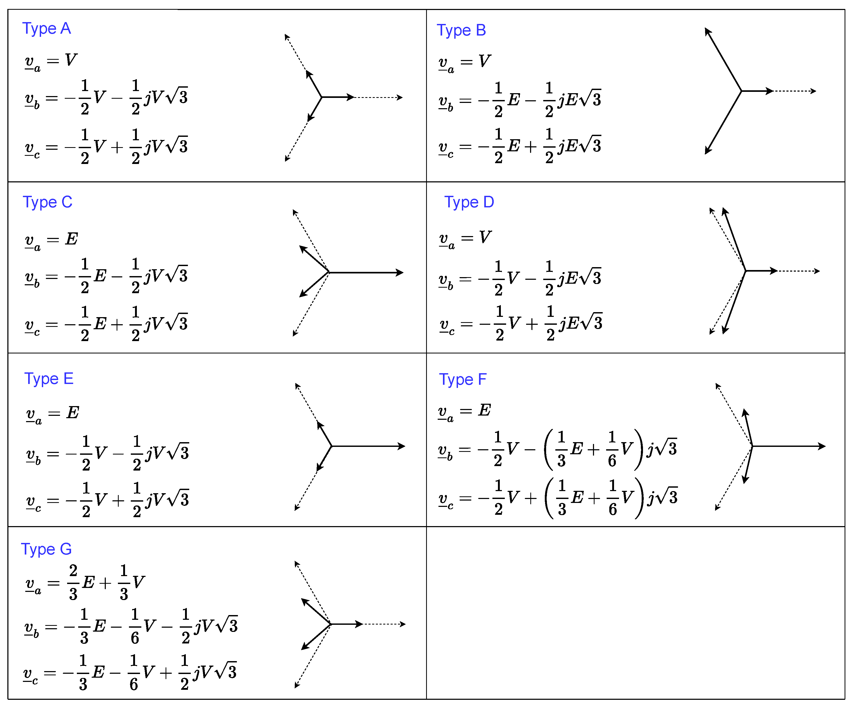
| Voltage Sag Type | Voltage Dip | ||||
|---|---|---|---|---|---|
| 0 pu | 0.20 pu | 0.40 pu | 0.60 pu | 0.80 pu | |
| A | 38% | 36% | 34% | 26% | 8% |
| B | 31% | 23% | 16% | 11% | 3% |
| C | 35% | 34% | 27% | 16% | 9% |
| D | 35% | 34% | 27% | 16% | 9% |
| E | 36% | 35% | 34% | 23% | 9% |
| F | 36% | 35% | 34% | 23% | 9% |
| G | 36% | 35% | 34% | 23% | 9% |
| Description | Parameter | Value |
|---|---|---|
| Nominal voltage (line-to-line) | 220 kV | |
| Resistance of the grid | ||
| Inductance of the grid | mH | |
| Resistance of the line | 7 × /m | |
| Inductive reactance of the line | 4 × /m | |
| Capacitive reactance of the line | 385 Mm | |
| Length of the line | 60 km | |
| Voltage ratio of the transformer | 260/220 kV | |
| Rated power of the transformer | 450 MVA | |
| Leakage inductance of the transformer | 47.82 mH (220 kV side) |
Disclaimer/Publisher’s Note: The statements, opinions and data contained in all publications are solely those of the individual author(s) and contributor(s) and not of MDPI and/or the editor(s). MDPI and/or the editor(s) disclaim responsibility for any injury to people or property resulting from any ideas, methods, instructions or products referred to in the content. |
© 2025 by the authors. Licensee MDPI, Basel, Switzerland. This article is an open access article distributed under the terms and conditions of the Creative Commons Attribution (CC BY) license (https://creativecommons.org/licenses/by/4.0/).
Share and Cite
Vidal-Albalate, R.; Belenguer, E.; Magraner, F. Modular Multilevel Converter Control Strategy for AC Fault Current Maximization and Grid Code Compliance. Electronics 2025, 14, 1763. https://doi.org/10.3390/electronics14091763
Vidal-Albalate R, Belenguer E, Magraner F. Modular Multilevel Converter Control Strategy for AC Fault Current Maximization and Grid Code Compliance. Electronics. 2025; 14(9):1763. https://doi.org/10.3390/electronics14091763
Chicago/Turabian StyleVidal-Albalate, Ricardo, Enrique Belenguer, and Francisco Magraner. 2025. "Modular Multilevel Converter Control Strategy for AC Fault Current Maximization and Grid Code Compliance" Electronics 14, no. 9: 1763. https://doi.org/10.3390/electronics14091763
APA StyleVidal-Albalate, R., Belenguer, E., & Magraner, F. (2025). Modular Multilevel Converter Control Strategy for AC Fault Current Maximization and Grid Code Compliance. Electronics, 14(9), 1763. https://doi.org/10.3390/electronics14091763