Computational Intelligence Approach for Fall Armyworm Control in Maize Crop

Abstract

This paper presents a method for dynamic pattern recognition and classification of one dangerous caterpillar species to allow for its control in maize crops. The use of dynamic pattern recognition supports the identification of patterns in digital image data that change over time. In fact, identifying fall armyworms (Spodoptera frugiperda) is critical in maize production, i.e., in all of its growth stages. For such pest control, traditional agricultural practices are still dependent on human visual effort, resulting in significant losses and negative impacts on maize production, food security, and the economy. Such a developed method is based on the integration of digital image processing, multivariate statistics, and machine learning techniques. We used a supervised machine learning algorithm that classifies data by finding an optimal hyperplane that maximizes the distance between each class of caterpillar with different lengths in N-dimensional spaces. Results show the method’s efficiency, effectiveness, and suitability to support decision making for this customized control context.

1. Introduction

Maize (Zea mays L.) is one of the most important agricultural crops and one of the most cultivated cereals in the world. There are signs of maize cultivation dating back approximately seven thousand years in the regions where the country of Mexico’s is located today. It was the main food source for the American people of that period [1,2].

According to the United States Department of Agriculture (USDA) [3], Brazil is the third largest maize producer in the world, with actual production of 122 million tons in an area of 21.5 million hectares in its 2023/2024 harvest and production forecasts of 127 million tons in an area of 22.30 million hectares for its 2024/2025 harvest. For comparison, the United States and China are ahead of Brazil in this regard, with forecast productions for their 2023/2024 harvests of 389.67 and 288.84 million tons, respectively.

A large range of pests and diseases attacks the maize crop during its different stages of plant development, which severely affects its productive potential [4]. Among other caterpillar pests, such as Helicoverpa armígera, Helicoverpa zea, and Elasmopalpus lignosellus Zeller [5], the fall armyworm (Spodoptera frungiperda) (FAW) is one of the most notorious and voracious, able to cause losses that could reach approximately 70% of production, as it attacks the plant still in its formation stage [6]. The extensive losses caused by this pest can heavily affect the economy, as it is also considered a serious pest for other important crops in the world, such as soybean, cotton, potato, etc. [7].

Table 1. Characteristics of caterpillars.

Type of Caterpillar	Specific Patterns	Color Patterns	Maximum Size (mm)
Spodoptera frungiperda	Inverted “Y” marking in the head area and four smaller dorsal spots in a trapeze arrangement on most segments and in a square arrangement on the last segment	Greenish to dark brown	40 mm
Helicoverpa armígera	Smooth saddle-shaped tubercles with hairs at the apex	Yellowish–white to reddish–brown or green	40 mm
Helicoverpa zea	Stripes of other colors arranged on the sides of the body	White and yellow, turning to brown	35 mm
Elasmopalpus lignosellus Zeller	Brown, purple, or dark-brown transverse streaks	Yellowish with red stripes; before hatching, it takes on a black coloration	22 mm

presents the specific patterns of the above-cited caterpillars and their particularities.

The first reports of FAW come from regions of North and South America, where it has been considered a constant pest [8]; however, in recent years, the presence of this pest has also been reported in different regions around the globe, including Asia [9], Africa [7], and Oceania [10]. In 2020, Kinkar et al. elaborated a technical report to the European Food Safety Authority (EFSA), where emergency measures were in place to prevent the introduction and spread of FAW within the European Union (EU). Due to the high spread capacity of adults, detection of moths at low levels of population is crucial to avoid further spread of this pest [11].

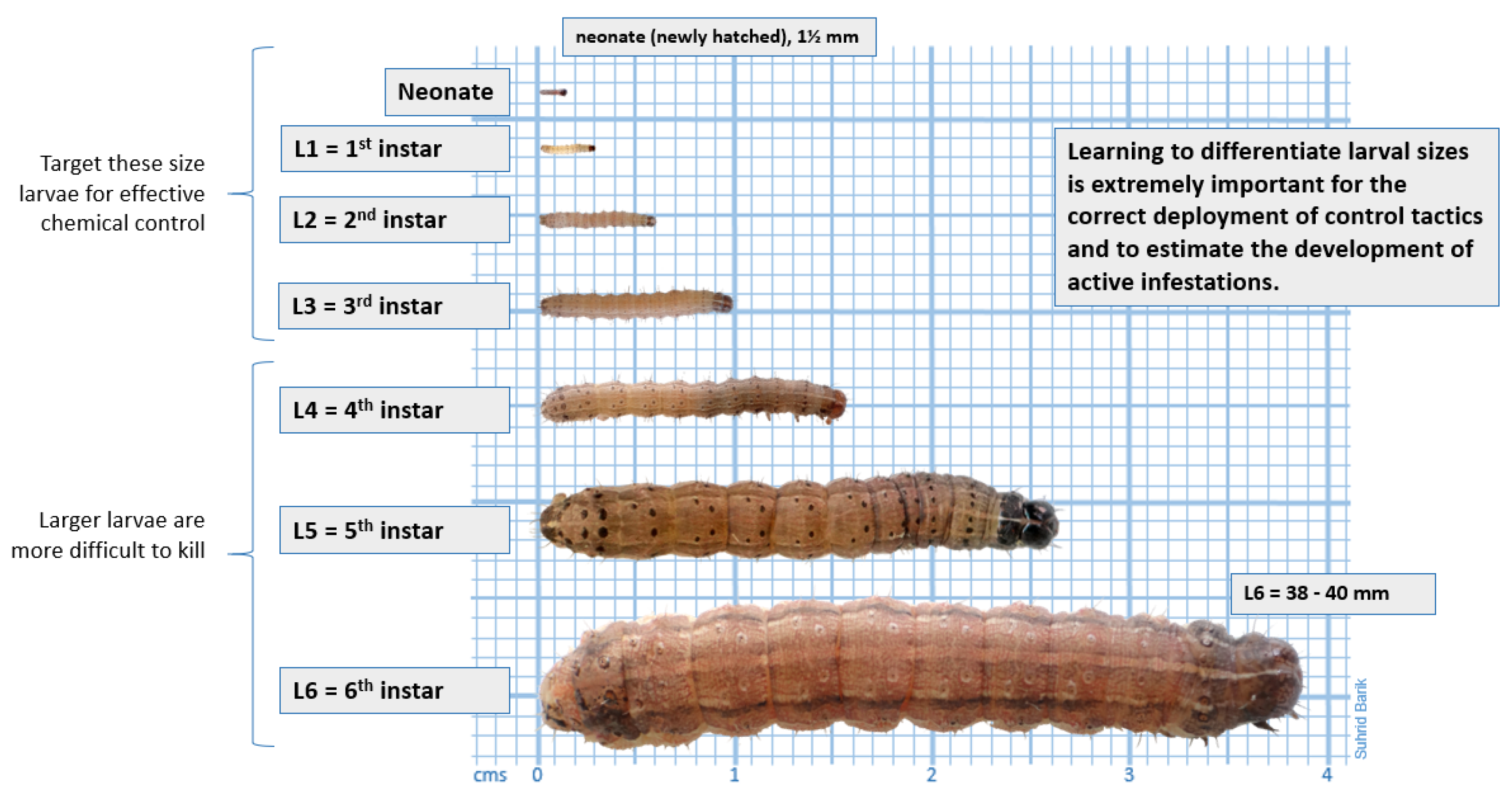
The developmental sequence of the FAW can be seen in Figure 1, which characterizes its different stages of growth, also called instars [5,12]. It is essential to emphasize that at about the neonate stage (newborn), given the size of the pest, it is impractical to attempt its detection by imaging; rather, it is more prudent to detect colonies (eggs).

However, according to agricultural pest experts, instars 5 and 6 can be regarded as a single instar based on their characteristics, method of control, and damage to the maize crop. Thus, the main focus of FAW pattern classification should be instars 1 to 5.

The current method of monitoring for FAW in maize includes trapping males using a pheromone odor similar to that of females. Once the pest is confirmed to be present in crop areas, insecticides are used for control.

However, such a technique can capture only the specimens that are already about to transform into moths or those that are already in that form, at which point they no longer cause significant damage to production [13]. Furthermore, traditional methods executed by humans are also labor-intensive and subjective, as they depend on human efforts [14].

This discrepancy between the current pest detection method and the intended result (to detect pests while they are still at their harmful stages) motivated this research study to find other methods for the early detection of this pest in cultured areas. Specifically, the focus of this study is on the development of a method for dynamic pattern recognition and classification for FAW based on the integration of digital image and signal processing, multivariate statistics, and machine learning (ML) techniques to favor the productivity of the maize crop.

The concept of computer vision seeks, through computer models, to reproduce the ability and functions of human vision, that is, the ability to see and interpret a scene. The ability to see can be implemented through the use of image acquisition devices and suitable methods for pattern recognition.

Nowadays, intelligent systems in agriculture that offer support for decisions in productive areas are equipped with capabilities based on machine learning processes. ML describes the capacity of systems to learn from customized problem-training data to automate and solve associated tasks [15,16,17]. In conjunction with such a concept, Deep learning (DL) is also a machine learning process but based on artificial neural networks with a set of specific-purpose layers [18,19]. The first layer of a neural network is the input layer, where the model receives input data. Such networks also include a convolutional layer, which uses filters to detect features in input data. In addition, to reduce the spatial dimensions of data, a pooling layer is used, which decreases the computational load. Likewise, after that, to allow for output, a fully connected layer is also included in such an arrangement, since each neuron in the layer is connected to every neuron in the previous and subsequent layer, which allows for analysis approaches [20].

Furthermore, ML and artificial intelligence (AI) can help in the decision-making process to establish a diagnosis with the aim of controlling this pest in a maize crop area. Currently, image and signal processing techniques are being utilized in several domains, most prominently in medicine [21], industry, security, and agriculture [22], among others.

Image acquisition has been verified to be a promising approach to the detection and identification of insect pests and plant diseases. In 2010, Sankaran et al. sought to identify diseased plants with greening or with nutritional deficiency through a method based on mid-infrared spectroscopy, where the samples are analyzed by a spectrometer [23]. In 2014, Miranda et al. proposed the study of different digital image processing techniques for the detection of pests in rice paddies by capturing images in the visible spectrum (RGB). They proposed a methodology in which images are scanned pixel by pixel both horizontally and vertically. This process is conducted in such a way that it is possible to detect and calculate the size (in pixels) of detected pests [24].

In 2015, Buades et al. presented a method for the filtering of digital images based on non-local means [25]. This method was compared with traditional methods of digital image filtering, such as Gaussian filtering, anisotropic diffusion filtering, and neighborhood-based filtering for white noise reduction. In 2011, Mythil and Kavitha compared the efficiencies of applying different types of filters to reduce noise in color digital images [26]. Mishra et al. compared Wiener, Lucy–Richardson, and regularized-filter digital filters to reduce noise in digital images [27].

In 2021, Bertolla and Cruvinel presented a method for the filtering of digital images degraded by non-stationary noise. In their research study, these authors added Gaussian-type noise with different levels of intensity to images of agricultural pests. Their approach allowed for the observation of images of maize pests with random noise signals for their [28] processing.

In 2013, He et al. highlighted methodologies based on image segmentation for the identification of pests and diseases in crops. With these methods, pests and diseases of cotton crops could be identified through segmentation techniques based on pseudo-colors (HSI and YCbCr), as well as in the visible spectrum (RGB) [29]. In 2015, Xia et al. detected small insect pests in low-resolution images that were segmented using the watershed method [30]. In 2017, Kumar et al. used the image segmentation technique known as adaptive thresholding for the detection and counting of insect pests. Such a method consists of computing the threshold of each pixel of the image by interpolating the results of the sub-images [31]. In 2018, Sriwastwa et al. compared color-based segmentation with Otsu segmentation and edge detection methods. Their experiments were initially performed with the Pyrilla pest (Pyrilla), found in sugarcane cultivation (Saccharum officinarum). Subsequently, the same methods were applied to images of termites (Isoptera) found in maize cultivation. For color-based segmentation, images were converted to the CIE L*a*b* [32] color space. For the feature extraction and pattern recognition of agricultural pests and diseases, in 2007, Huang applied an artificial neural network with the backpropagation algorithm for the classification of bacterial soft rot (BSR), bacterial brown spot (BBS), and Phytophthora black rot (PBR) in orchid leaves. The color and texture characteristics of the lesion area caused by the diseases were extracted using a co-occurrence matrix [33].

In 2011, Sette and Mailard proposed a method based on texture analysis of georeferenced images for the monitoring of a certain region of the Atlantic Forest based on images analyzed in the visible spectrum. Metrics such as contrast, entropy, correlation, inverse moment of difference, and second angular momentum were also extracted from the co-occurrence matrix [34].

On the other hand, machine learning-based approaches were discussed in 2008 by Ahmed et al., who then developed a real-time machine vision-based methodology for the recognition and control of invasive plants. The proposed system also had the objective of recognizing and classifying invasive plants into broad-leaf and narrow-leaf classes based on the measurement of plant density through masking operations [35].

In 2012, Guerrero et al. proposed a method based on a support vector machine (SVM) classifier for identification of weeds in maize plantations. For the classification process, they used SVM classifiers with a polynomial kernel, radial basis function (RBF), and sigmoid function [36].

In 2015, for the classification of different leaves, Lee et al. used a Convolutional Neural Network (CNN) based on the AlexNet neural network and a deconvolutional network to observe the transformation of leaf characteristics. For the detection of pests and diseases in tomato cultivation, a methodology based on machine learning techniques was proposed by Fuentes et al. [37]. Three models of neural networks were used to perform this task. To recognize pests and diseases (objects of interest) and their locations in the plant, faster region-based convolutional neural networks (F-CNNs) and region-based fully convolutional neural networks (R-FCNs) have been used [38].

In 2017, Thenmozhi and Reddy presented digital image processing techniques for insect detection in the early stage of sugar cane crops based on the extraction of nine geometrical features. The authors used the Bugwood image database for image sample composition [39]. In 2023, the same image database was used by Tian et al. The authors proposed a model based on the deep learning architecture to identify nine kinds of tomato diseases [40]. In 2019, Evangelista proposed the classification of flies and mosquitoes based on the frequency of their wing beats. Fast Fourier transform and a Bayesian classifier were used [41].

In 2018, Nanda et al. proposed a method for detecting termites based on SVM classifiers, using pieces of wood previously divided into two classes: infested and not infested by termites. SVM classifiers with linear kernel, RBF, polynomial, and sigmoid functions were used on datasets obtained by microphones, which captured sound signals from termites [42]. In 2019, Lui et al. presented a methodology for extracting data from intermediate layers of CNNs with the purpose of using these data to train a classifier and, thus, make it more robust. Features extracted from the intermediate layers of a CNN were representative and could significantly improve the accuracy of the classifier. To test the effectiveness of that method, CNNs such as AlexNet, VggNet, and ResNet were used for feature extraction. The extracted features were used to train classifiers based on SVM, naive Bayes, linear discriminant analysis (LDA), and decision trees [43].

In 2019, Li et al. trained a maximum likelihood estimator for the classification of maize grains. “Normal” and “damaged” classes were defined, the latter having seven subclassifications [44]. In 2019, Abdelghafour et al. presented a framework for classifying the covers of vines in their different phenological stages, that is, foliage, peduncle, and fruit. For this task, a Bayesian classifier and a probabilistic maximum a posteriori (MAP) estimator were used [45].

In 2022, Moreno and Cruvinel presented results related to the control of weed species with instrumental improvements based on a computer vision system for direct precision spray control in agricultural crops for the identification of invasive plant families and their quantities [46].

In 2024, Wang and Luo proposed a method to identity specific pests that occur in maize crops. This method is based on a YOLOv7 network and the SPD-Conv module to replace the convolutional layer, i.e., to realize small target feature and location information. According to the authors, the experimental results showed that the improved YOLOv7 model was more efficient for such control [47].

In 2024, Liu et al. proposed a model to detect maize leaf diseases and pests. These authors presented a multi-scale inverted residual convolutional block to improve models’ ability to locate the desired characteristics and to reduce interference from complex backgrounds. In addition, they used a multi-hop local-feature architecture to address problems regarding the extraction of features from images [48].

In 2025, Valderrama et al. presented an ML method to detect Aleurothrixus floccosus in citrus crops. This method is based on random sampling image acquisition, i.e., alternating the extraction of leaves from different trees. Techniques of imaging processing, including noise reduction, edge smoothing, and segmentation, were also applied. The final results were acceptable, and the authors used a dataset of 1200 digital images for validation [17].

Also in 2025, Zhong et al. proposed a flax pest and disease detection method for different crops based on an improved YOLOv8 model. The authors employed the Albumentations library for data augmentation and a Bidirectional Feature Pyramid Network (BiFPN) module. This arrangement was organized to replace the original feature extraction network, and the experimental results demonstrated that the improved model achieved significant detection performance on the flax pest and disease dataset [49].

This paper presents the integration of digital image processing, multivariate statistics, and computational intelligence techniques, focusing on a method for dynamic pattern recognition and classification of FAW caterpillars. Customized context analysis is also performed, taking into account ML and DL based on SVM classifiers and an AlexNet CNN (A-CNN) [50] through the use of the Tensorflow framework.

After this Introduction, the remainder of this paper is organized as follows: Section 2 introduces the materials and methods, Section 3 presents the results and respective discussions, and Section 4 provides conclusions and includes suggestions for continuity and future research.

2. Materials and Methods

All experiments were performed in Python (version 3.11), i.e., by using both the image processing and ML libraries in openCV, as well as the scikit-image and scikit-learn algorithms. We also considered an operating platform with a 64-bit CPU Intel (R) model Core(TM) i7-970, 16 Gb RAM, and Microsoft Windows 11 operating system. Figure 2 shows a block diagram of the method for classifying the patterns of FAW caterpillars.

Concerning the dataset used for validation, the choice of images was based mainly on their quality and diversity. For this study, the Insect Images dataset, which is a subset of the Bugwood Image Database System, was selected. Currently, the Bugwood Image Database System is composed of more than 300 thousand images divided into more than 27 thousand subgroups. Another important factor for the use of this dataset is that most of the images were captured in the field, that is, they were influenced by lighting and have variations in scale and size, among other characteristics resulting from acquisition in a real environment. Therefore, in order to minimize the effects of lighting on the images, a set of digital images from leaves and cobs with the presence of FAW was taken into account, acquired under close lighting intensities, in addition to the inclusion of geometric feature extraction, together with color and texture information, for pattern recognition.

Table 2. Characteristics of images of fall armyworm (Spodoptera frugiperda) in Insect Image dataset.

Type of Archive	JPG/JPEG
Color space	RGB
Image width	3072 pixels
Image height	2048 pixels
Image resolution	72 ppi (pixels per inch)
Pixel size	≈0.35 mm

outlines the characteristics of the images used to validate the developed method.

The restoration process considers the use of a degradation function (H), resulting in a restored image ($f^{\prime }(x,y)$). When the degradation is exclusively due to noise, the H function is applied with a value equal to 1. On the other hand, a filter ($g(x,y)$) enables an image to be obtained such that it presents a better result in terms of the Signal-to-Noise Ratio (SNR). As a result, a restored image ($\widehat{f}(x,y)$) is obtained. The process of restoring noisy images can be applied to both the spatial and frequency domains.

For noise filtering of the acquired images, the use of digital filters and the presence of noise, mainly random Gaussian and impulsive noises, were considered [51]. In digital image processing, noise can be defined as any change in the signal that causes degradation or loss of information from the original signal, which can be caused by lighting conditions of the scene or object, the temperature of the signal capture sensor during the acquisition of the image, or transmission of the image, among other factors [28].

For the problem regarding FAW, it has been observed that only noises present in the considered images need to be treated. Thus, H equals 1, and additive noises resulting from temperature variation of the image capture sensor and influenced by lighting conditions can be represented as follows:

$$\widehat{f}(x,y)=\eta (x,y)+f(x,y),$$

(1)

where $f(x,y)$ represents the original image, $\eta (x,y)$ is the noise added to the original image, and $\widehat{f}(x,y)$ is the noisy image [26,52].

In this work, image restoration was performed in the spatial domain. The use of Gaussian filters [53] and non-local means [25] was evaluated. The application of a Gaussian filter has the effect of smoothing an image; the degree of smoothing is controlled by the standard deviation ($\sigma$). Its kernel follows the mathematical model expressed as follows:

$$f(x,y)={\displaystyle \frac{1}{2\pi {\sigma }^2}}{exp}^{\left(-{\displaystyle \frac{x^2+y^2}{2{\sigma }^2}}\right)},$$

(2)

where x and y represent the kernel dimensions of the filter and $\sigma$ is the value of the standard deviation of the Gaussian function with $\sigma >0$.

The application of a non-local mean (NLM) filter is based, as the name suggests, on non-local mean measures. The NLM filter searches for the estimated value of the intensity of each pixel (i) in a certain region of the image (f), then calculates the weighted average of this region. The similarity is estimated according to an image with noise (g) in the form of $g\left(i\right)|i\in f,NL{M}_{\left[g\right]\left(s\right)}$, where $NLM$ represents the estimated value of a given pixel (i) [54] as follows:

$$NL{M}_{\left[g\right]\left(s\right)}={\displaystyle \frac{1}{C_{\left(i\right)}}}\sum _{j\in f}\omega (i,j)g\left(j\right),$$

(3)

where $C_{\left(i\right)}$ is a normalizing factor, i.e., $C_{\left(i\right)}\ne 0$, and $\omega (i,j)$ represents the similarity of the weights of pixels i and j to satisfy the conditions of $0\le \omega (i,j)\le 1$ and ${\sum }_{j\in f}\omega (i,j)=1$. In addition, the weight of $\omega (i,j)$ [55] is calculated as follows:

$${\omega }_{(i,j)}={\displaystyle \frac{1}{C_{\left(i\right)}}}{exp}^{-{\displaystyle \frac{|{\left(N_i\right)}^2-{\left(N_j\right)}^2|}{{\sigma }^2}}},$$

(4)

where $N_i$ and $N_j$ are vectors of pixels whose values are related not only to similarity measures but also to the Gaussian weighted Euclidean distance at which intensities of the gray levels are within a square neighborhood centered at positions i and j, respectively.

For color-space operations, the use of the HSV and CEI L*a*b* color spaces was evaluated based on images acquired in the RGB color space [56].

In reference to digital image processing, the RGB color space applies mainly to the image acquisition and result visualization stages. However, because of its low capacity to capture intensity variation in color components [57], its use is not recommended in the other stages of the process.

To convert an RGB image to the HSV color space, because of the more natural representation of RGB colors for human perception, it is necessary to normalize the values of the R, G, and B components, measuring their respective maximum and minimum values, then convert them to the HSV color space as follows:

$$\begin{array}{c}\hfill \begin{array}{c}H=\left\{\begin{array}{ccc}{60}^{°}-\left({\displaystyle \frac{G^{\prime }-B^{\prime }}{\Delta }}mod6\right)\hfill & \mathrm{if}& C_{max}=R^{\prime }\\ {60}^{°}-\left({\displaystyle \frac{B^{\prime }-R^{\prime }}{\Delta }}+2\right)\hfill & \mathrm{if}& C_{max}=G^{\prime }\\ {60}^{°}-\left({\displaystyle \frac{R^{\prime }-G^{\prime }}{\Delta }}+4\right)\hfill & \mathrm{if}& C_{max}=B^{\prime }\end{array}\right.\end{array},\end{array}$$

(5)

$$\begin{array}{c}S=\left\{\begin{array}{ccc}0& \mathrm{if}& \Delta =0\\ {\displaystyle \frac{\Delta }{C_{max}}}& \mathrm{if}& \Delta \ne 0\end{array}\right.\end{array},$$

(6)

$$V=C_{max},$$

(7)

where $C_{max}$ is the maximum value of the R, G, and B components; $C_{min}$ is the minimum value of the R, G, and B components; and H, S, and V are the components of the HSV color space.

It is also possible to convert images from the HSV to the RGB color space, considering the following:

$$\begin{array}{c}(R_1,G_1,B_1)=\left\{\begin{array}{ccc}(C,X,0)& \mathrm{if}& 0^{°}\le H<{60}^{°}\\ (X,C,0)& \mathrm{if}& {60}^{°}\le H<{120}^{°}\\ (0,C,X)& \mathrm{if}& {120}^{°}\le H<{180}^{°}\\ (0,X,C)& \mathrm{if}& {180}^{°}\le H<{240}^{°}\\ (X,0,C)& \mathrm{if}& {240}^{°}\le H<{300}^{°}\\ (C,0,X)& \mathrm{if}& {300}^{°}\le H<{360}^{°}\end{array}\right.\end{array},$$

(8)

where $R_1$, $G_1$, and $B_1$ represent points on the faces of the RGB cube, whereas C represents the chroma component.

On the other hand, the conversion from the RGB to the CIE L*a*b* color space follows the method described below. The Commission Internationale de l’Eclairage (CIE), or the International Commission on Illumination, defines the sensation of color based on the elements of luminosity, hue, and chromaticity. Thus, the condition of existence of color is based on three elements: illuminant, object, and observer [58]. Accordingly, the color space known as CIE Lab started to consider the “L” component as a representation of luminosity, ranging from 0 to 100; the “a” component as a representation of chromaticity, ranging from green (negative values) to red (or magenta for positive values); and the “b” component also as a representation of chromaticity, varying from yellow (for negative values) to blue (or cyan for positive values) [59]. In 1976, the CIE L*a*b* standard was created based on improvements of the CIE Lab created in 1964. The new standard provides more accurate color differentiation concerning human perception [60]. However, given that the old standard is still widely used, the use of asterisks (∗) was adopted in the nomenclature of the new standard.

Because the CIE L*a*b* color space standard, like its predecessor, is based on the CIE XYZ color standard, conversion from RGB images occurs in two steps [61]. First, the RGB image is converted to the CIE XYZ standard, that is,

$$\left[\begin{array}{c}X\\ Y\\ Z\end{array}\right]=\left[\begin{array}{ccc}0.4125& 0.3576& 0.1804\\ 0.127& 0.7152& 0.0722\\ 0.0193& 0.1192& 0.9502\end{array}\right]\left[\begin{array}{c}R\\ G\\ B\end{array}\right].$$

(9)

Once the image has been converted to the CIE XYZ standard, it can be converted to the CIE L*a*b* standard, considering the following:

$$\begin{array}{c}{L}^{*}=\left\{\begin{array}{ccc}116{\left({\displaystyle \frac{Y}{Y_n}}\right)}^{{\displaystyle \frac{1}{3}}}-16& \mathrm{if}& {\displaystyle \frac{Y}{Y_n}}>0.008856\\ \\ 903,3\left({\displaystyle \frac{Y}{Y_n}}\right)& \mathrm{if}& {\displaystyle \frac{Y}{Y_n}}\le 0.008856\end{array}\right.\end{array},$$

(10)

$$\begin{array}{c}{a}^{*}=500\left[\begin{array}{c}{\left({\displaystyle \frac{X}{X_n}}\right)}^{{\displaystyle \frac{1}{3}}}-{\left({\displaystyle \frac{Y}{Y_n}}\right)}^{{\displaystyle \frac{1}{3}}}\end{array}\right]\end{array},$$

(11)

$$\begin{array}{c}{b}^{*}=200\left[\begin{array}{c}{\left({\displaystyle \frac{X}{X_n}}\right)}^{{\displaystyle \frac{1}{3}}}-{\left({\displaystyle \frac{Z}{Z_n}}\right)}^{{\displaystyle \frac{1}{3}}}\end{array}\right]\end{array}.$$

(12)

The segmentation step aims to divide, or isolate, regions of an image, which could be labeled as foreground and background objects. Thus, foreground objects are called regions of interest (ROIs) of the image, that is, regions where patterns related to the end objective are sought for the identification of FAW. Background objects are any other objects that are not of interest [62].

Segmentation algorithms are generally based on two basic properties: discontinuity, such as edge detection and the identification of borders between regions, and similarity, which is the case of pixel allocation in a given region [63].

In binary images, the representation of pixels with values of 0 (black) normally indicates the background of the image, whereas that of pixels with values of 1 (white) indicates the object(s) of interest [64].

A binary image ($b(x,y)$) is generated with the application of a threshold (T) to the histogram of the original image ($f(x,y)$), considering the following:

$$b(x,y)=\left\{\begin{array}{ccc}0,& \mathrm{if}& f(x,y)<T\\ 1,& \mathrm{if}& f(x,y)\ge T\end{array}\right..$$

(13)

The threshold value can be chosen through a manual analysis from the histogram of an image or the use of an automatic threshold selection algorithm. In this case, seed pixels were used. Additionally, the use of Otsu’s method was considered. This method performs non-parametric and unsupervised discriminant analysis and automatically selects the optimal threshold based on the intensity values of the pixels of a digital image, allowing for a better separation of classes [65].

In a 2D digital image with dimensions of $N\times M$ and an intensity level of L, where $n_i$ denotes the number of pixels of intensity i, and $MN$ is the total number of pixels, the histogram is normalized considering the following [66]:

$$p_i={\displaystyle \frac{n_i}{MN}},$$

(14)

where $p_i\ge 0$ and ${\sum }_{i=1}^L{p}_i=1$.

The operation of a threshold ($T\left(k\right)=k$, where $0<k<L-1$) divides the L intensity levels of an image into two classes ($C_1$ and $C_2$, representing the object of interest and the background of the image, respectively, where $C_1$ consists of all pixels in the range of $[0,k]$ and $C_2$ covers the range of $[k+1,L-1]$). This operation is defined as follows:

$$P_1\left(k\right)=\sum _{i=0}^k{p}_i,$$

(15)

where $P_1\left(k\right)$ is the probability of a pixel (k) being assigned to class $C_1$.

Likewise, the probability of occurrence of class $C_2$ is expressed as follows:

$$P_2\left(k\right)=\sum _{i=k+1}^{L-1}{p}_i=1-P_1\left(k\right).$$

(16)

The values of the average intensities of classes $C_1$ and $C_2$ are given considering the following equations:

$$m_1\left(k\right)=\sum _{i=0}^{k}iP\left(i\right|C_1)={\displaystyle \frac{1}{P_1\left(k\right)}}\sum _{i=0}^{k}i{p}_i,$$

(17)

$$m_2\left(k\right)=\sum _{i=k+1}^{L-1}iP\left(i\right|C_2)={\displaystyle \frac{1}{P_2\left(k\right)}}\sum _{i=k+1}^{L-1}i{p}_i.$$

(18)

The average cumulative intensity ($m\left(k\right)$) is expressed as follows:

$$m\left(k\right)=\sum _{i=0}^{k}i{p}_i.$$

(19)

The optimal threshold can be obtained via the minimization of one of the discriminant functions, described as follows:

$$\lambda ={\displaystyle \frac{{\sigma }_B^2}{{\sigma }_W^2}},\eta ={\displaystyle \frac{{\sigma }_B^2}{{\sigma }_G^2}},\kappa ={\displaystyle \frac{{\sigma }_T^2}{{\sigma }_W^2}},$$

(20)

where ${\sigma }_W^2$ is within-class variance, ${\sigma }_B^2$ is cross-class variance, and ${\sigma }_G^2$ is global variance, respectively expressed as follows:

$${\sigma }_B^2=P_1{P}_2{(m_1-m_2)}^2={\displaystyle \frac{{(m_G{P}_1-m)}^2}{P_1(1-P_1)}},$$

(21)

$${\sigma }_G^2=\sum _{i=0}^{L-1}{(i-m_G)}^{2}pi.$$

(22)

The greater the difference in the average values of $m_1$ and $m_2$, the greater the variance between classes (${\sigma }_B^2$), confirming it to be a separability measure [66]. Likewise, if ${\sigma }_G^2$ is a constant, it is possible to verify that $\eta$ is also a measure of separability and that maximizing this metric is equivalent to maximizing ${\sigma }_B^2$. Thus, the objective is to determine the value of k to maximize the variance between classes. Therefore, the threshold (k) that maximizes the $\eta$ function is selected based on the following:

$$\eta \left(k\right)={\displaystyle \frac{{\sigma }_B^2\left(k\right)}{{\sigma }_T^2}}.$$

(23)

Also, when the optimal threshold ($k^{*}$) is obtained, the original image ($f(x,y)$) is segmented considering the following:

$$b(x,y)=\left\{\begin{array}{ccc}0,& \mathrm{if}& f(x,y)\le k^{*}\\ 1,& \mathrm{if}& f(x,y)>k^{*}\end{array}\right..$$

(24)

The use of Otsu’s method automates the process of segmenting images containing objects that represent FAW both in maize leaves and cobs. Additionally, after the segmentation method was applied, the extraction of features from these patterns, through the use of the methods of the histogram of oriented gradient (HOG) [67] and invariant moments of Hu [68], was considered.

Herein, the HOG descriptor is applied in five stages [69]. The first involves transforming the segmented image in the CIE L*a*b* color space to grayscale (in 8-bit or 256-tone conversion), whereas the other steps involve calculating the intensities of the gradients; grouping the pixels of the image into cells; grouping these cells into blocks; and, finally, extracting characteristics of the magnitude of the gradient, according to the following equation:

$$m(x,y)=\sqrt{{\left[f_u(x,y)\right]}^2+{\left[f_v(x,y)\right]}^2},$$

(25)

where m is the magnitude of the feature vector at point $(x,y)$. Additionally, $f_u(x,y)$ consists of a component in u directions, and $f_v(x,y)$ is a component in v directions. It is possible to obtain the direction of the gradient vector ($\theta (x,y)$) in the following form:

$$\theta (x,y)={tan}^{-1}{\displaystyle \frac{f_v(x,y)}{f_u(x,y)}}.$$

(26)

In addition, for geometrical feature extraction purposes, the Hu invariant moments descriptor was considered [70]. First, it is necessary to calculate the two-dimensional moments. They can be defined as polynomial functions projected in a 2D image ($f(x,y)$) with dimensions of $M\times N$ and order $(p+q)$.

The normalized central moments allow the central moments to be invariant-to-scale transformations, defined as follows:

$${\eta }_{pq}={\displaystyle \frac{{\mu }_{pq}}{{\mu }_{00}^{\gamma }}},$$

(27)

where $\gamma$ is defined as

$$\gamma ={\displaystyle \frac{p+q}{2}}+1,$$

(28)

for $p+q=2,3,\dots$, positive integers ∈$\mathbb{Z}$.

Then, the invariant moments can be calculated as follows:

$${\varphi }_1={\eta }_{20}+{\eta }_{02},$$

(29)

$${\varphi }_2={({\eta }_{20}-{\eta }_{02})}^2+4{\eta }_{11}^2,$$

(30)

$${\varphi }_3={({\eta }_{30}-3{\eta }_{12})}^2+{(3{\eta }_{21}-{\eta }_{03})}^2,$$

(31)

$${\varphi }_4={({\eta }_{30}+{\eta }_{12})}^2+{({\eta }_{21}+{\eta }_{03})}^2,$$

(32)

$$\begin{array}{c}{\varphi }_5=({\eta }_{30}-3{\eta }_{12})({\eta }_{30}+{\eta }_{12})[{({\eta }_{30}+{\eta }_{12})}^2-3{({\eta }_{21}+{\eta }_{03})}^2]+\\ (3{\eta }_{21}-{\eta }_{03})({\eta }_{21}+{\eta }_{03}),\end{array}$$

(33)

$$\begin{array}{c}{\varphi }_6=({\eta }_{20}-{\eta }_{02})[{({\eta }_{30}+{\eta }_{12})}^2-{({\eta }_{21}+{\eta }_{03})}^2]+\\ 4{\eta }_{11}({\eta }_{30}+{\eta }_{12})({\eta }_{21}+{\eta }_{03}),\end{array}$$

(34)

$$\begin{array}{c}{\varphi }_7=(3{\eta }_{21}-{\eta }_{03})({\eta }_{30}+{\eta }_{12})[{({\eta }_{30}+{\eta }_{12})}^2-3{({\eta }_{21}+{\eta }_{03})}^2]+\\ (3{\eta }_{12}-{\eta }_{30})({\eta }_{21}+{\eta }_{03})[3{({\eta }_{30}+{\eta }_{12})}^2-{({\eta }_{21}+{\eta }_{03})}^2].\end{array}$$

(35)

Furthermore, in this work, we used Principal Component Analysis (PCA) [71] to reduce the dimensionality of the vector. We consider a data array (X) with n observations and m independent variables.

$$\mathbf{X}=\left[\begin{array}{ccc}{x}_{11}& \cdots & x_{1m}\\ ⋮& \ddots & ⋮\\ x_{n1}& \cdots & x_{nm}\end{array}\right].$$

(36)

The principal components can be measured as a set of m variables ($X_1$, $X_2$, …, $X_m$) with means (${\mu }_1$, ${\mu }_2$, …, ${\mu }_m$) and variance (${\sigma }_1^2$, ${\sigma }_2^2$, …, ${\sigma }_m^2$), in which covariance between the n-th and m-th variables takes the following form:

$$\mathsf{\Sigma }=\left[\begin{array}{ccc}{\sigma }_{11}^2& \cdots & {\sigma }_{1m}^2\\ ⋮& \ddots & ⋮\\ {\sigma }_{n1}^2& \cdots & {\sigma }_{nm}^2\end{array}\right],$$

(37)

where $\mathsf{\Sigma }$ is the covariance matrix. Eigenvalues and eigenvectors are measured ((${\lambda }_1,e_1$), (${\lambda }_2,e_2$), …, (${\lambda }_m,e_m$), where ${\lambda }_1\ge {\lambda }_2\ge \dots \ge {\lambda }_m$) and associated with $\Sigma$, where the i-th principal component is defined as follows:

$$Z_i=e_{i1}{X}_1+e_{i2}{X}_2+\dots +e_{im}{X}_m,$$

(38)

where $Z_i$ is the ith principal component. The objective is to maximize the variance of $Z_i$ as follows:

$$Var\left(Z_i\right)=Var\left(e_i^{\prime }\mathbf{X}\right)=e_i^{\prime }Var\left(\mathbf{X}\right)e_i=e_i^{\prime }\mathsf{\Sigma }{e}_i,$$

(39)

where i = 1, …, m. Thus, the spectral decomposition of the matrix ($\mathsf{\Sigma }$) is expressed as $\mathsf{\Sigma }=\mathbf{P}\mathsf{\Lambda }{\mathbf{P}}^{\prime }$, where P is the composite matrix according to the eigenvectors of $\mathsf{\Sigma }$ and $\mathsf{\Lambda }$ is the diagonal matrix of eigenvalues of $\mathsf{\Sigma }$. Thus,

$$\mathsf{\Lambda }=\left[\begin{array}{cccc}{\lambda }_1& 0& \cdots & 0\\ 0& {\lambda }_2& \cdots & 0\\ ⋮& ⋮& \ddots & ⋮\\ 0& 0& \cdots & {\lambda }_m\end{array}\right].$$

(40)

The principal component of greatest importance is defined as the one with the greatest variance that explains the maximum variability in the data vector, as the second highest variance represents the second most important component, and so on, to the least important component.

The vector of reduced dimensionality features is composed of normalized eigenvectors, representing the descriptors of the FAW descriptors in the images. The feature vector comprises the input data for pattern recognition, involving ML.

As mentioned previously, in other words, ML may also be understood as the ability of a computational system to improve performance in a task based on experience [72]. In this work, the classification technique is related to ML—specifically, supervised learning [73]. Supervised learning is based on existent and classified patterns serving as training examples that enable a classifier to be efficiently generalized to new datasets [18]. In this context, the feature vector, with reduced dimensionality, is used for classification according to its position in the feature space.

In this work, after having defined the feature vector, as a next step, the application of computational intelligence is considered, i.e., based not only on SVM classifiers [74] but also taking into account the A-CNN through the use of the Tensorflow framework [19,75] for evaluation. In such a way, it is possible to carry out a context evaluation to choose between the use of ML or DL models in such a customized pest control problem.

SVM classifiers were selected for use in this study, since they have been quite well used for the classification of agricultural data, as reported in [76]. SVMs can be established based on linear behavior or even non-linear behavior. In this work, two types of kernel that are associated with these functionalities were evaluated to determine which one leads to the best operability, accuracy, precision, and other parameters associated with the analysis of the behaviors of these classifiers [77].

Classifiers with linear behavior use a hyperplane that maximizes the separation between two classes from a training dataset (x) with n objects ($x_i\in \mathbf{X}$) and their respective labels ($y_i\in \mathbf{Y}$) such that X represents the input dataset and $\mathbf{Y}=(-1,+1)$ represents possible classes [72]. In this case, the hyperplane is defined as follows:

$$\begin{array}{cc}{y}_i(\mathbf{w}·{\mathbf{x}}_i+b)-1\ge 0,& \forall ({\mathbf{x}}_i,y_i)\in \mathbf{X}\end{array},$$

(41)

where w is the normal vector to the hyperplane, $\mathbf{w}·\mathbf{x}$ is the dot product of vectors w and x, and b is a fit term.

The maximization of the data separation margin in relation to $\mathbf{w}·\mathbf{x}+b=0$ can be obtained via the minimization of $∥\mathbf{w}∥$ [78]. The minimization problem is quadratic because the object function is quadratic and the constraints are linear. This problem can be solved via the introduction of the Lagrange function [79]. The Lagrange function must be minimized concerning w and b, implying the maximization of the variables (${\alpha }_i$). The value of L is derived concerning w and b.

This formulation is referred to as the dual form, whereas the original problem is referred to as the primal form. The dual form presents simpler restrictions and allows for the representation of the optimization problem in terms of inner products between data, which are useful for the nonlinearization of SVMs. It is also worth noting that the dual problem uses only training data and their labels [72].

Linearly separable datasets are classified efficiently by linear SVMs, with some error tolerance in the case of a linear SVM with smooth margins. However, in several cases, it is not possible to efficiently classify training data using this modality of a hyperplane [72], requiring the use of interpolation functions that allow for operation in larger spaces, that is, using non-linear SVM classifiers.

In that manner, it is possible for SVMs to deal with non-linear problems through a $\mathsf{\Phi }$ function, mapping the dataset from its original space (input space) to a larger space (input space characteristics) [80], characterizing a non-linear SVM classifier.

Thus, based on the choice of $\Phi$, the training dataset (x), in its input space ($R^2$), is scaled to the feature space ($R^3$) as follows:

$$\mathsf{\Phi }\left(x\right)=\Phi (x_1,x_2)=(x^2,\sqrt[2]{2}{x}_1{x}_2,x_2^2),$$

(42)

$$h\left(\mathbf{x}\right)=\mathbf{w}·\mathsf{\Phi }\left(\mathbf{x}\right)+b=w_1{x}_1^2+w_2\sqrt[2]{2}{x}_1{x}_2+w_3{x}_2^2+b=0.$$

(43)

In this way, the data are initially mapped to a larger space; then, a linear SVM is applied over the new space. A hyperplane is then found with a greater margin of separation, ensuring better generalization [81].

Given that the feature space can be in a very high dimension, the calculation of $\mathsf{\Phi }$ might be extremely costly or even unfeasible. However, the only necessary information about the mapping is the calculation of the scalar products between the data in the feature space obtained through function kernels [72].

Table 3. Selected kernels to validate the developed method.

Kernel	Function $\mathit{K}\mathbf{(}{\mathit{x}}_{\mathit{i}}\mathbf{,}{\mathit{x}}_{\mathit{j}}\mathbf{)}$	Parameters
Polynomial	${(\delta ({\mathbf{x}}_i·{\mathbf{x}}_j)+\kappa )}^d$	$\delta$, $\kappa$ e d
Radial basis function (RBF) kernel	$exp(-\sigma {∥{\mathbf{x}}_i-{\mathbf{x}}_j∥}^2)$	$\sigma$
Sigmoidal	tanh($\delta$(${\mathbf{x}}_i$·${\mathbf{x}}_j$) + $\kappa$)	$\delta$ e $\kappa$

presents the kernels selected to validate the developed method.

For each type of kernel, one should define a set of parameters, which must be customized as a function of the problem to be solved.

In addition, the use of a CNN based on a tensor is evaluated, which can be defined as a mathematical entity used for multidimensional representation of data. Its order determines the indices required for the component’s access. In fact, tensors can be scalar, vectors, matrices, or even higher-order entries with N dimensions [82], as follows:

$$\begin{array}{c}\mathbf{X}\in {\mathbf{R}}^{I_{1}x{I}_{2}x\dots I_N}\end{array},$$

(44)

where $I_k$ for $1\le k\le N$ is the dimension of the k-th mode of the tensor and $x_{i_1,i_2,\dots ,i_N}$ denote each element of the tensor (X).

A Tensor Network (TN) is defined as a collection of tensors that can be multiplied or compacted according to a predefined topology. In such an arrangement, the configuration can be obtained by taking into account two types of indices. One of them considers a linked index, which can connect tensors two at a time to structure the network arrangement. The other uses an open index, which makes it possible to connect tensors directly to the network being structured. Larger scale dimensions can also be obtained by using addition and multiplication operations and considering linked and open operators, respectively.

In this work, all parameters are considered, not only for the SVM classifiers but also for the A-CNN, to allow for control of FAW caterpillars in maize crops.

3. Results and Discussions

For this study, an image dataset of the FAW in maize crop was organized, with a total of 2280 images representing its five stages of development, that is, 456 images generated for each stage of development. Figure 3 shows the results of the image acquisition step.

Based on the mean squared error (MSEs) and peak signal-to-noise ratios (PSNRs) of the images restored by the spatial filtering process, it was observed that the NLM filter yielded a better result than the Gaussian filter, as shown in Figure 4.

Table 4. Non-local mean filter parameters and values.

Parameter	Value
Kernel	$7\times 7$
Patch width	11
Patch height	11

presents the parameters used for the application of the NLM filter. These parameters were obtained after several tests performed with this filter based on the available literature.

The use of a kernel with dimensions of $7\times 7$ pixels and a height and distance patch of 11 pixels allowed for the maximum attenuation of medium- and low-frequency noise effects, as well as the maintenance of the textural characteristics of the images.

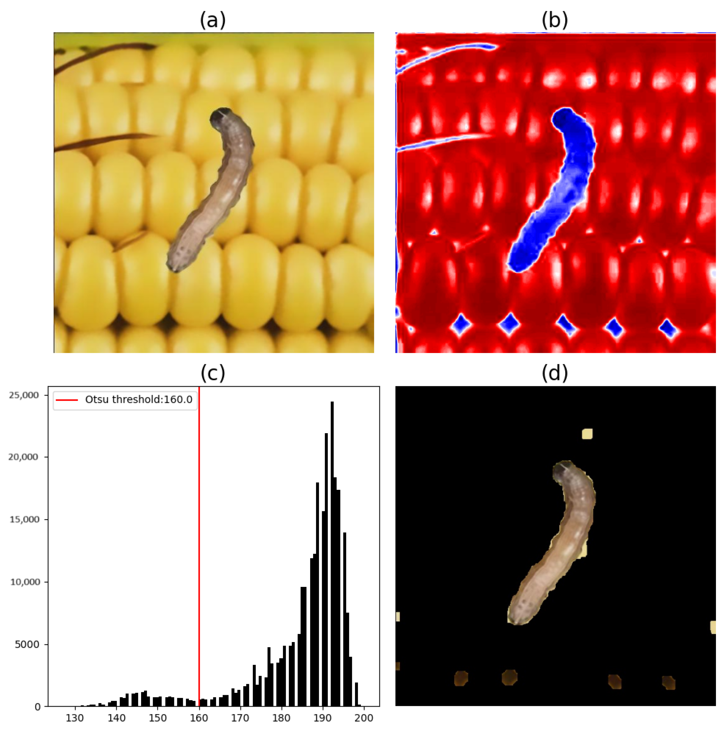
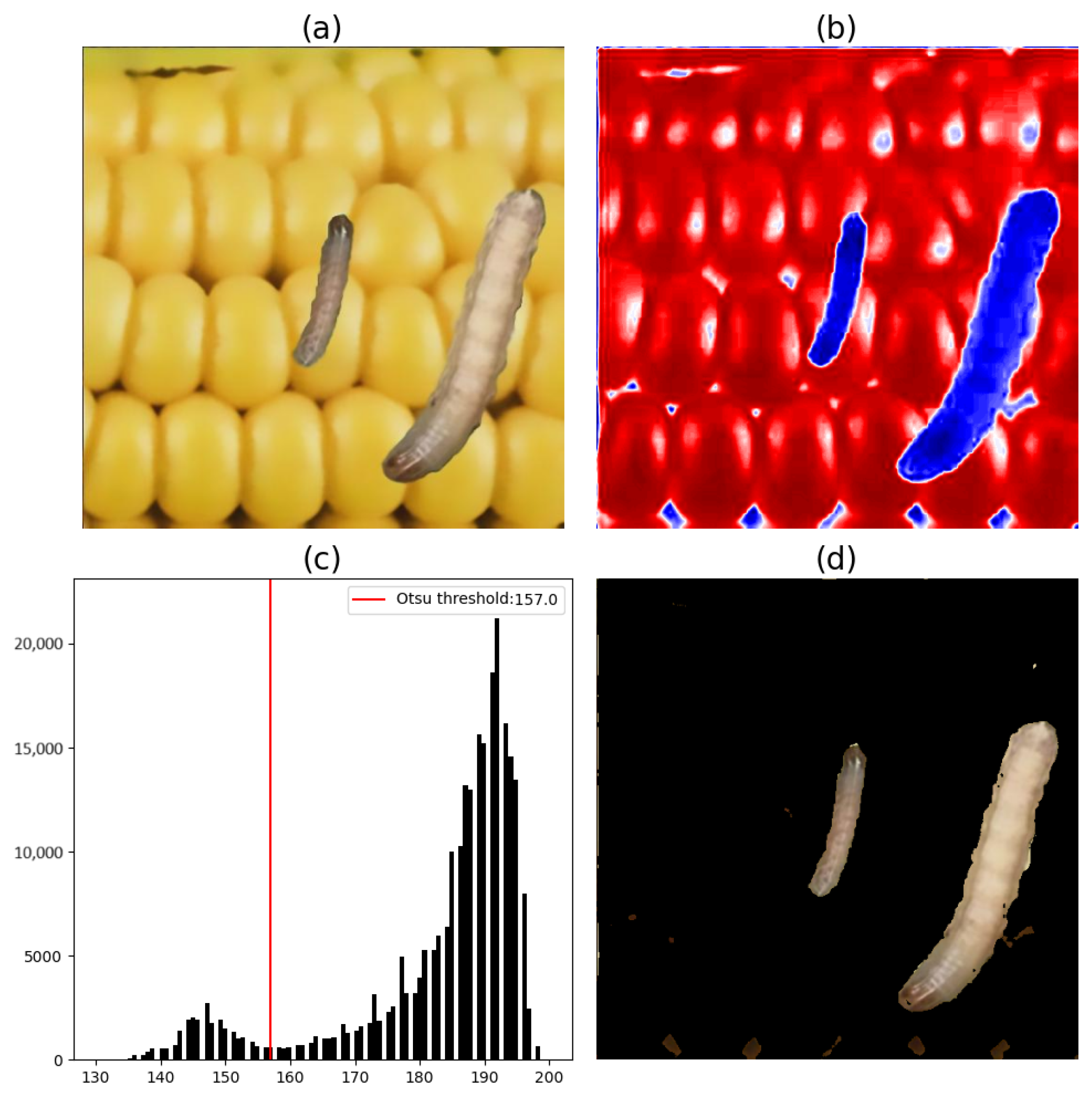
For the image segmentation stage, tests were conducted using Otsu’s method based on the conversion of the HSV and CIE L*a*b* color spaces. However, because of the verified restrictions for the H map of the HSV color space, it was decided that the CIE L*a*b* would be used instead to obtain an ideal segmentation process.

Figure 5, Figure 6 and Figure 7 illustrate the image segmentation process using Otsu’s method based on components a* and b*, where each image shows only one FAW found on the considered region of maize leaves.

Figure 8, Figure 9 and Figure 10 illustrate the image segmentation process using Otsu’s method and based on components a* and b*, where each image showed two FAWs found on the considered region of maize leaves.

When the histograms of the a* components of Figure 5 and Figure 8 are analyzed, it can be seen that the pixels with the lowest values, represented by the blue color, refer to the pixels of maize plant leaves. Conversely, the highest-value pixels, in red, represent pest pixels and other anomalies present on the leaf. Therefore, to segment the pest from the rest of the image, only pixels with values above the threshold obtained by Otsu’s method are considered.

However, based on the tests conducted on the segmentation of images of FAWs on leaves using Otsu’s method and only the a* component of the CIE L*a*b* color space, it was determined that, despite the proven efficiency of this segmentation method, there is an evident need for a second segmentation stage. Assays were then performed using the b* component.

In histogram analysis of Figure 6 and Figure 9, it can be seen that the pixels with the lowest values represent the pixels of the pest and some parts of the leaf. Therefore, to segment the pest from the rest of the image, only pixels with values below the threshold obtained by Otsu’s method were considered.

Approximating the segmentation process using only the a* component, segmentation using the b* component also resulted in an image with parts of the leaf still in it. However, it was possible to verify that, in the spatial domain of the image, the non-segmented parts referring to the leaf in the segmentation with the a* component did not belong to the same spatial locations as the segmentation result achieved by the b* component. Therefore, based on the results obtained via the segmentation of the pest from the image on a leaf by the a* and b* components of the CIE L*a*b* color space, a new segmentation step was performed, this time in the form of an intersection. It can be observed from the results that segmentation by intersection proved to be efficient in the segmentation of images of pests on leaves.

Figure 11 and Figure 12 illustrate the image segmentation process using Otsu’s method and based on the b* components of FAWs found in the considered region of maize cobs. In Figure 11, only one FAW caterpillar is shown. In Figure 12, two FAW caterpillars in different stages are shown.

For the segmentation of the FAW on maize cobs using Otsu’s method, the results of the tests performed on the a* component of the CIE L*a*b* color space are shown to be inefficient, given the conversion process from the RGB color space. Thus, for the segmentation of pests on maize cobs, only the b* component was used.

The histograms of the map of the b* component (Figure 11 and Figure 12) show that the highest-value pixels represent the maize cob pixels in the b* component. Thus, to segment the FAW caterpillars from all the collected images, pixels with values below the threshold obtained by Otsu’s method were considered.

The results of the segmentation process showed that parts of the cob were not completely segmented. These results were expected for the segmentation of both images with spikes and images containing leaves because during the tests performed to validate the segmentation step of the standard method, the complexity of image formation was verified in terms of the two values of the pixels that constitute both the FAW and the background of the image.

Thus, it could be verified that for images of FAW caterpillars found on leaves, the segmentation process using Otsu’s method and the a* and b* maps achieved a result considered ideal, whereas for images of FAW caterpillars found on cobs, only the segmentation using the map of the b* component was sufficient.

In relation to image descriptors, in this work, we considered the use of the HOG and Hu methodologies.

The HOG descriptor was used to extract texture features of the FAW.

Table 5. HOG descriptor parameters.

Parameter	Value
Pixels per cell	$16\times 16$
Cells per block	$2\times 2$
Numbers of orientations	9
Feature vector	TRUE
Transform SQRT	FALSE

displays the parameterization of the HOG descriptor.

For the execution of the HOG descriptor, previously segmented images were resized to obtain a spatial resolution of $256\times 256$ pixels. Once the parameters of the HOG descriptor were applied to the resized images, it was possible to generate a feature vector of 8100 positions in the form of $V_{\left[HOG\right]}$ for each image of the FAW, as illustrated in Figure 13.

Once the feature vector ($V_{\left[HOG\right]}$) was obtained through the use of the HOG descriptor, the Hu invariant moment descriptor was then applied to the FAW images, as demonstrated in Figure 14.

Thus, for each image of the FAW, a feature vector ($V_{\left[Hu\right]}$) was generated, containing the seven invariant moments of Hu, that is, the shape and size features of the pests: M₁, M₂, M₃, M₄, M₅, M₆, and M₇.

Considering the obtained descriptors, one referring to texture characteristics (HOG) and another referring to geometric characteristics (Hu), it was possible to classify the patterns of the FAW in its different stages of development after applying PCA to reduce the feature vector.

In fact, in feature extraction using the HOG descriptor and the Hu invariant moment descriptor, the feature vectors ($V_{\left[HOG\right]}$ and $V_{\left[Hu\right]}$) were concatenated to generate a single vector of features ($V_{[HOG,Hu]}$) with 8107 positions, as illustrated in Figure 15.

Therefore, because the values referring to texture, shape, and size characteristics are in different scales, it was necessary to normalize them before the generation of a database with the characteristic features of the patterns presented in each analyzed image.

Furthermore, by using PCA, it was possible to achieve a dimensionality reduction from 2280 to 128 principal components, maintaining approximately 98% of the variability of the original data, as shown in Figure 16.

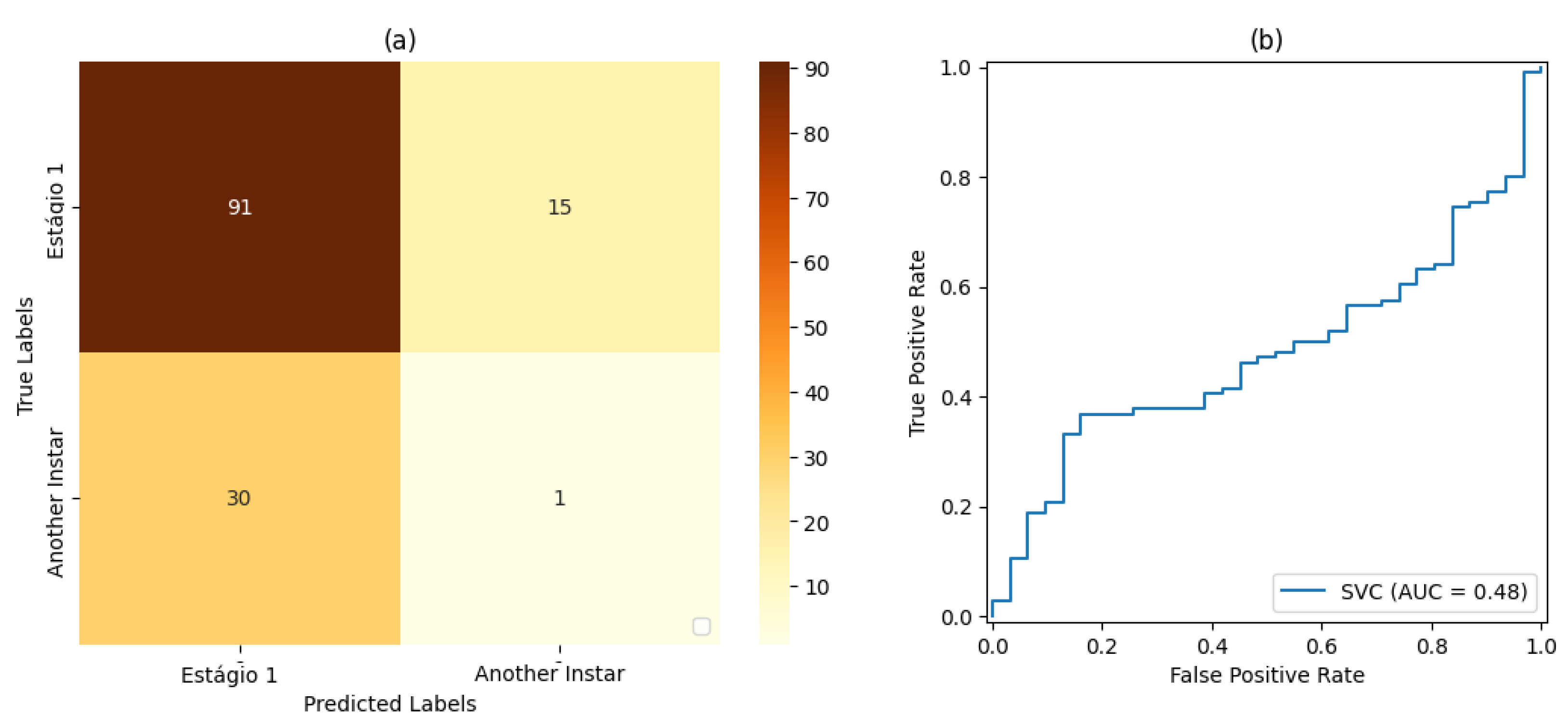
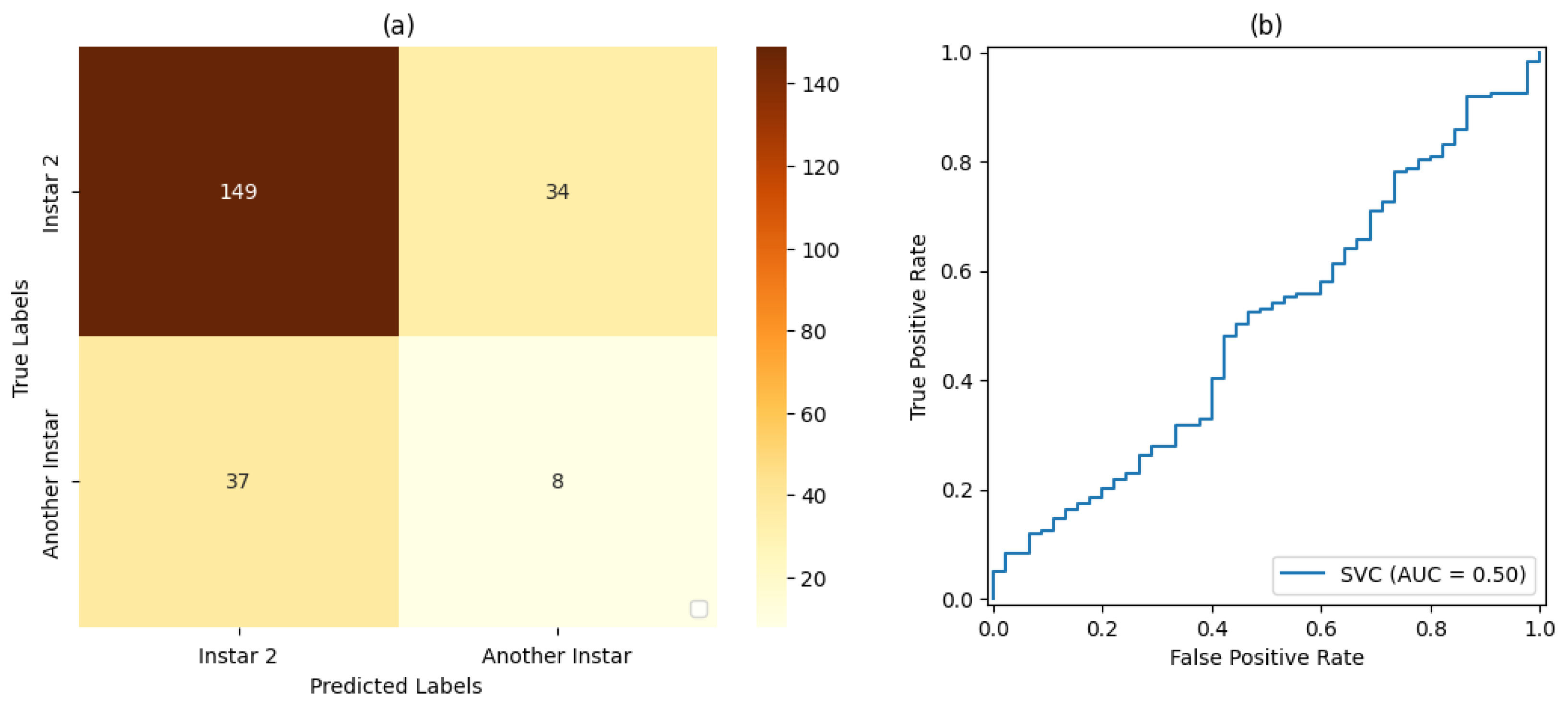
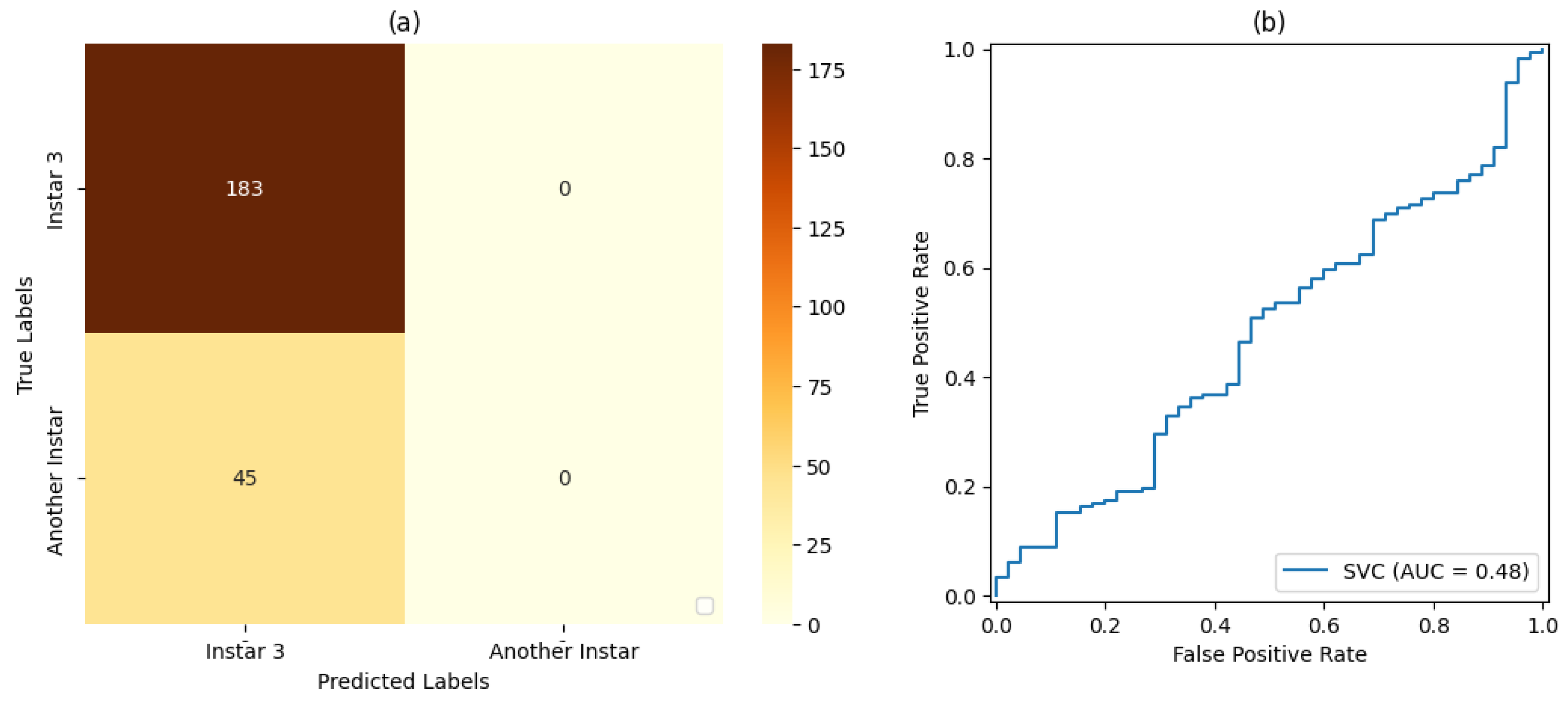
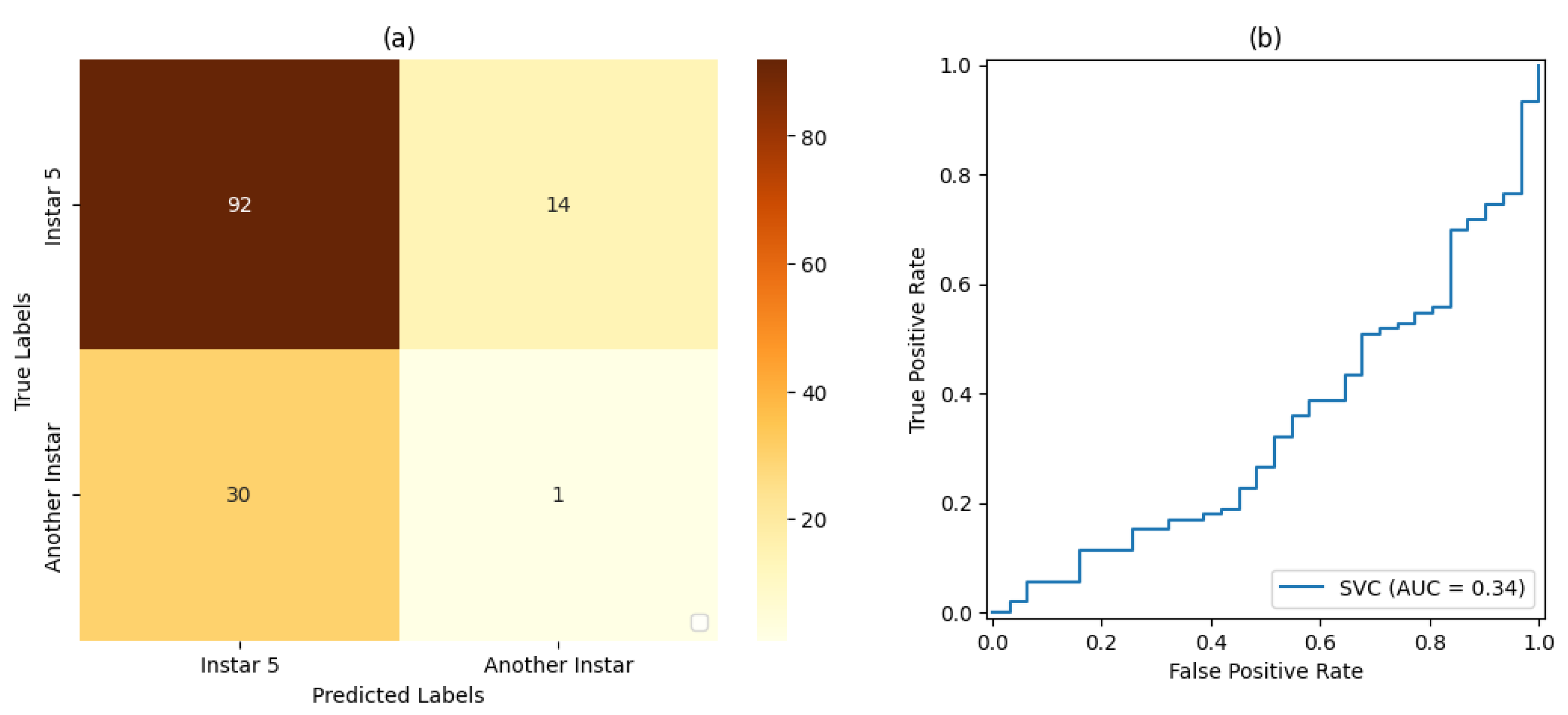
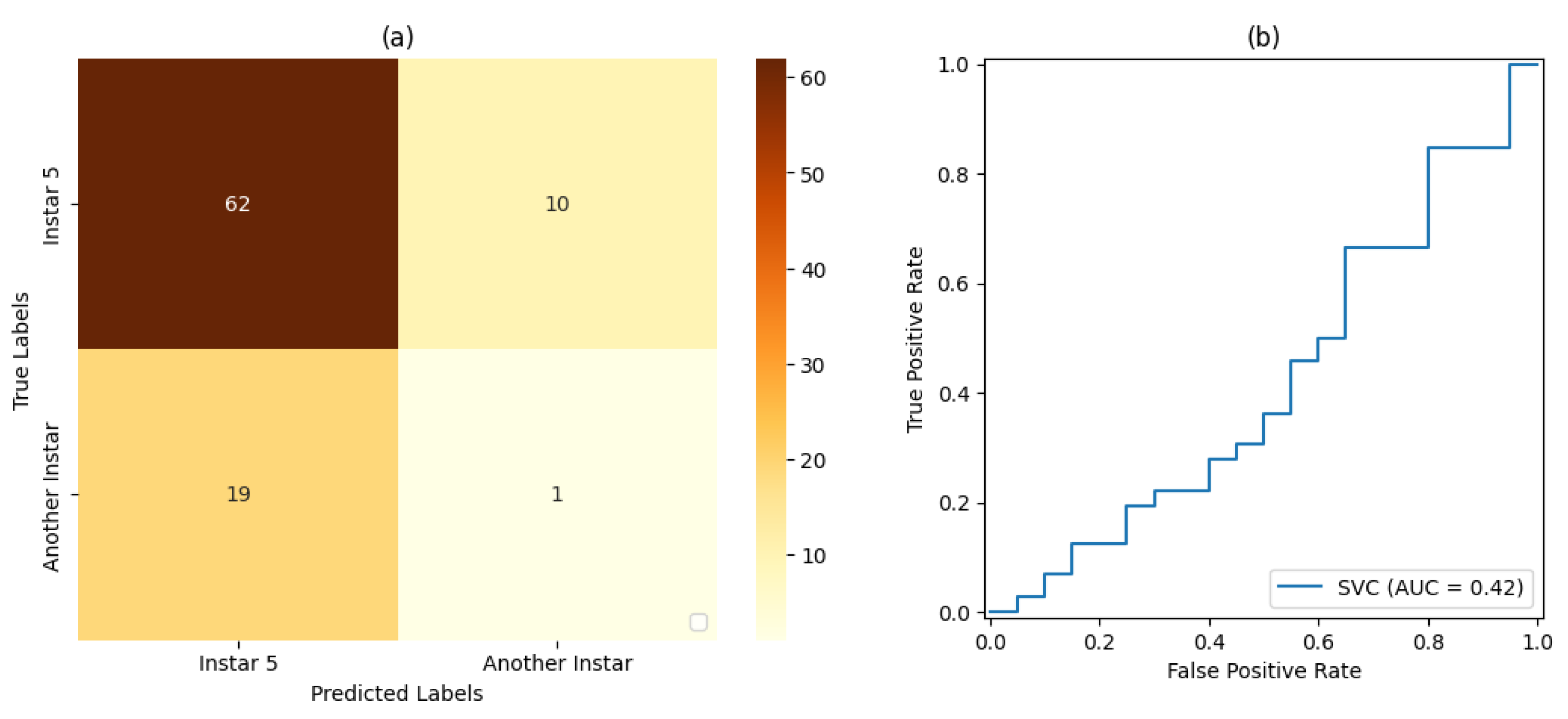
In the tests on the classification and ML stage, SVM classifiers with a linear kernel function and a sigmoid kernel function were considered. For the validation of each SVM classifier, both the accuracy and precision in classifying the FAW target stage were taken into account.

For the training and testing stages of the SVM classifiers and the CNN, dataset proportions of 50%:50%, 70%:30%, and 80%:20% were evaluated for training and testing, respectively.

Table 6. Fall armyworm stage classification with SVM linear function kernel and dataset proportion of 50% for training and testing.

SMV Classifier	Precision	Recall	F1 Score	Support Vectors	Accuracy (%)
# 1	0.81	0.63	0.71	183	0.59
# 2	0.83	0.69	0.75	183	0.64
# 3	0.73	0.79	0.83	183	0.73
# 4	0.85	0.79	0.82	183	0.72
# 5	0.85	0.72	0.78	183	0.68

,

Table 7. Fall armyworm stage classification with SVM linear function kernel and dataset proportions of 70% for training and 30% for testing.

SMV Classifier	Precision	Recall	F1 Score	Support Vectors	Accuracy (%)
# 1	0.74	0.68	0.71	106	0.56
# 2	0.78	0.65	0.71	106	0.57
# 3	0.82	0.79	0.80	106	0.70
# 4	0.81	0.78	0.80	106	0.69
# 5	0.86	0.75	0.80	106	0.71

, and

Table 8. Fall armyworm stage classification with SVM linear function kernel and dataset proportions of 80% for training and 20% for testing.

SMV Classifier	Precision	Recall	F1 Score	Support Vectors	Accuracy (%)
# 1	0.71	0.61	0.66	72	0.50
# 2	0.72	0.65	0.69	72	0.53
# 3	0.79	0.81	0.80	72	0.68
# 4	0.81	0.78	0.79	72	0.68
# 5	0.82	0.75	0.78	72	0.67

present the results of SVM classifiers with a linear kernel function and dataset proportions of 50% for training and testing, 70% for training and 30% for testing, and 80% and 20% for training and testing, respectively.

Table 9. Fall armyworm stage classification with SVM sigmoidal function kernel and dataset proportion of 50% for training and testing.

SMV Classifier	Precision	Recall	F1 Score	Support Vectors	Accuracy (%)
# 1	0.80	0.87	0.83	183	0.72
# 2	0.80	0.81	0.81	183	0.68
# 3	0.80	1.00	0.89	183	0.80
# 4	0.81	0.99	0.89	183	0.80
# 5	0.80	0.85	0.82	183	0.71

,

Table 10. Fall armyworm stage classification with SVM sigmoidal function kernel and dataset proportions of 70% for training and 30% for testing.

SMV Classifier	Precision	Recall	F1 Score	Support Vectors	Accuracy (%)
# 1	0.75	0.86	0.86	106	0.67
# 2	0.77	0.83	0.80	106	0.68
# 3	0.77	1.00	0.87	106	0.77
# 4	0.77	0.99	0.87	106	0.77
# 5	0.75	0.87	0.81	106	0.89

, and

Table 11. Fall armyworm stage classification with SVM sigmoidal function kernel and dataset proportions of 80% for training and 20% for testing.

SMV Classifier	Precision	Recall	F1 Score	Support Vectors	Accuracy (%)
# 1	0.77	0.88	0.82	72	0.70
# 2	0.80	0.86	0.81	72	0.69
# 3	0.78	1.00	0.88	72	0.78
# 4	0.78	0.97	0.86	72	0.76
# 5	0.77	0.86	0.81	72	0.68

present the results of the SVM classifiers with sigmoidal kernel functions and dataset proportions of 50%:50%, 70%:30%, and 80%:20% for training and testing, respectively.

Taking into account the classifiers having linear and sigmoidal function kernels, the assessed results revealed their efficiency in the dynamic classification of the FAW. It was possible to observe that the best results were obtained by using the sigmoidal function kernel. Therefore, a deeper evaluation of the SVM classifier based on such a function kernel was considered as follows.

For stage 1, the SVM classifier with a proportion 50%:50% of the dataset for training and testing presented the best result, with an accuracy rate of 72% and a precision rate of 80%. For stage 2, the SVM classifier with a proportion of 80%:20% of the dataset for training and testing, respectively, showed the best results based on precision and accuracy of 80% and 69%, respectively. For stage 3, the SVM classifier with a proportion of 50% of the dataset for training and testing showed the best result, with 80% accuracy and precision. For stage 4, the best result was demonstrated by the SVM classifier with a proportion of 50% of the dataset for training and testing. Finally, for stage 5, the SVM classifier that presented the best result was also the classifier with a proportion of 50% of the dataset for training and testing, resulting in 71% accuracy and 80% precision.

Figure 17, Figure 18 and Figure 19 illustrate the confusion matrices and ROC curves for the performance of Classifier $\#1$.

Based on the measurements of the false-positive rate and true-positive rate, the AUC measures resulting from each version of Classifier $\#1$ could be analyzed. In this way, it could be verified that the proportion of 50% of the dataset used for training and testing led to the best result in relation to the classifiers set for this work placement, i.e., $AUC=52\%$, followed by the classification with a proportion of 70%:30% of the dataset used for training and testing, respectively, with $AUC=48\%$. The classification with a proportion of 80%:20% of the dataset used for training and testing, respectively, led to the result of $AUC=45\%$.

Figure 20, Figure 21 and Figure 22 illustrate the confusion matrices and ROC curves for Classifier $\#2$.

For Classifier $\#2$, for the produced AUC measures, it was observed that the classifier with a proportion of 50% of the dataset used for training and testing obtained the best result in relation to the classifiers set for this work placement, i.e., $AUC=50\%$, followed by the classification with a proportion of 80%:20% of the dataset used for training and testing, respectively, with $AUC=49\%$. The classification with a proportion of 70%:30% of the dataset used for training and testing, respectively, obtained a result of $AUC=45\%$.

Figure 23, Figure 24 and Figure 25 illustrate the confusion matrices and ROC curves for Classifier $\#3$.

For Classifier $\#3$, for the produced AUC measures, it was observed that the classifier with a proportion of 50% of the dataset used for training and testing presented a result of $AUC=48\%$, and the same result was achieved for classification with a proportion of 70%:30% of the dataset used for training and testing, respectively. The classification with a proportion of 80%:20% of the dataset used for training and testing, respectively, achieved a result of $AUC=44\%$.

Figure 26, Figure 27 and Figure 28 illustrate the confusion matrices and ROC curves for Classifier $\#4$.

With regard to Classifier $\#4$, the classifiers with a proportion of 50% of the dataset used for training and testing presented the best result in relation to the classifiers set for this work placement, i.e., $AUC=49\%$, followed by the classification with a proportion of 70%:30% of the dataset used for training and testing, respectively, with $AUC=43\%$. The classification with a proportion of 80%:20% of the dataset used for training and testing, respectively, achieved a result of $AUC=35\%$.

Figure 29, Figure 30 and Figure 31 illustrate the confusion matrices and ROC curves for Classifier $\#5$.

In relation to Classifier $\#5$, for the produced AUC measures, it was observed that the classification with a proportion of 50% of the dataset used for training and testing presented the best result in relation to the classifiers set for this work placement, i.e., $AUC=45\%$, followed by the classification with a proportion of 80%:20% of the dataset used for training and testing, respectively, with $AUC=42\%$. The classification with 70%:30% of the dataset used for training testing, respectively, achieved a result of $AUC=34\%$.

It was also observed that, even in some cases where the metrics of the confusion matrix and the ROC curve showed considerable rates of false positives and false negatives, the classification rate of true-positive values was significantly more accurate. Such behavior can be explained by the fact that all images included the pest and that, even at different stages of development, its shape, size, and texture characteristics are similar.

Since the use of SVM classifiers was useful in the methodology for FAW recognition and classification, a deep analysis was carried out in order to select the best parameters. In terms of time consumption for training and testing, the best proportion among the presented results is 70% for training and 30% for testing, as illustrated in

Table 12. Selected SVM classifiers for fall armyworm (Spodoptera frugperda) image pattern classification.

SVM Classifier	Kernel Function	Parameter C	Parameter Delta ($\mathit{\delta }$)
# 1	Sigmoidal	10	1,0
# 2	Sigmoidal	100	1,0
# 3	Sigmoidal	0.1	0.1
# 4	Sigmoidal	0.1	10
# 5	Sigmoidal	1	1

.

Additionally, analyses with the same proportions of data split were carried out on the CNN for FAW classification. In this scenario, for hidden layers, the ReLU function activation was selected and as the final activation function for the output layer, and the Softmax function was applied. The considered number of epochs was equal to twelve.

Table 13. Fall armyworm stage classification with A-CNN and dataset proportion of 50% for training and testing.

Instar	Precision	Recall	F1 Score	Accuracy (%)
# 1	0.84	0.83	0.83	0.90
# 2	0.96	0.69	0.80	0.90
# 3	0.80	1.00	0.89	0.90
# 4	0.95	0.95	0.95	0.90
# 5	1.00	1.00	1.00	0.90

,

Table 14. Fall armyworm stage classification with A-CNN and dataset proportion of 70% for training and 30% for testing.

Instar	Precision	Recall	F1 Score	Accuracy (%)
# 1	0.55	0.97	0.70	0.83
# 2	1.00	0.13	0.23	0.83
# 3	1.00	0.99	0.99	0.83
# 4	0.94	1.00	0.97	0.83
# 5	1.00	1.00	1.00	0.83

, and

Table 15. Fall armyworm stage classification with A-CNN and dataset proportions of 80% for training and 20% for testing.

Instar	Precision	Recall	F1 Score	Accuracy (%)
# 1	0.88	0.94	0.91	0.84
# 2	1.00	0.80	0.89	0.84
# 3	0.60	1.00	0.85	0.84
# 4	0.98	0.51	0.67	0.84
# 5	1.00	0.97	0.98	0.84

present the results obtained using the A-CNN with dataset proportions of 50%:50%, 70%:30%, and 80%:20% for testing and testing, respectively.

Figure 32, Figure 33 and Figure 34 illustrate the confusion matrices and ROC curves for the results obtained using the A-CNN.

Table 16. Comparison of fall armyworm classification with SVM and A-CNN using a dataset proportion of 50% for training and testing.

Instar	SVM Accuracy (%)	CNN Accuracy (%)	SMV Precision	CNN Precision
# 1	0.72	0.90	0.80	0.84
# 2	0.68	0.90	0.80	0.96
# 3	0.80	0.90	0.80	0.80
# 4	0.80	0.90	0.91	0.95
# 5	0.71	0.90	0.80	1.00

,

Table 17. Comparison of fall armyworm classification with SVM and the A-CNN using dataset proportions of 70% for training and 30% for testing.

Instar	SVM Accuracy (%)	CNN Accuracy (%)	SMV Precision	CNN Precision
# 1	0.67	0.83	0.75	0.55
# 2	0.68	0.83	0.77	1.00
# 3	0.77	0.83	0.77	1.00
# 4	0.77	0.83	0.77	0.94
# 5	0.89	0.83	0.75	1.00

, and

Table 18. Comparison of fall armyworm classification with SVM and the A-CNN using dataset proportions of 80% for training and 20% for testing.

Instar	SVM Accuracy (%)	CNN Accuracy (%)	SMV Precision	CNN Precision
# 1	0.70	0.84	0.77	0.88
# 2	0.69	0.84	0.80	1.00
# 3	0.78	0.84	0.78	0.60
# 4	0.76	0.84	0.78	0.98
# 5	0.68	0.84	0.77	1.00

present comparisons of SVM classifiers and the A-CNN based on precision and accuracy, with dataset proportions of 50%:50%, 70%:30%, and 80%:20% training and testing, respectively.

For the configurations presented as options for the computational intelligence stage, both for the use of SVM classifiers (with an ML focus) and for the use of the A-CNN (with a DL focus), percentages of 50:50%, 70:30%, and 80:20% were considered for training and testing, respectively. For such a context, both the confusion matrix and the respective ROC curves were observed in order to evaluate the information regarding precision and accuracy for all different instars of the FAW caterpillar.

Taking into account these results, it was possible to observe the following. For instar #1 the best configuration was obtained using the A-CNN with a proportion of 50%:50% for testing and training, respectively, leading to an accuracy equal to 90% and a precision equal to 84%. For instar #2, the best configuration was obtained using the A-CNN with a proportion of 50%:50% for testing and training, respectively, leading to an accuracy equal to 90% and a precision equal to 96%. For instar #3, the best configuration was obtained using the A-CNN with a proportion of 50%:50% for testing and training, respectively, leading to an accuracy equal to 90% and a precision equal to 80%. It is important to observe that for instar #3, the resulting precision value, when using the SVM classifier, was equal to that achieved by the A-CNN; however, the accuracy value was smaller. For instar #4, the best configuration was obtained using the A-CNN with a proportion of 50%:50% for testing and training, respectively, leading to an accuracy equal to 90% and a precision equal to 95%. For instar #5, the best configuration was obtained using the A-CNN with a proportion of 50%:50% for testing and training, respectively, leading to an accuracy equal to 90% and a precision equal to 100%.

Table 19. A-CNN parametrization for fall armyworm (Spodoptera frugperda) image pattern classification.

Instar	Hidden-Layer Activation Function	Output-Layer Activation Function	Epochs
# 1	ReLU	Softmax	10
# 2	ReLU	Softmax	10
# 3	ReLU	Softmax	10
# 4	ReLU	Softmax	10
# 5	ReLU	Softmax	10

presents the final parametrization for the A-CNN to classify the different instars of FAW caterpillars.

Furthermore, Figure 35 illustrates the resultant context analysis considering the use of both ML and DL for FAW caterpillar classification purposes, focusing its control in a maize crop area. It was possible to observe that the structure that considers ML with SVM classifiers solved the problem in a good way, including gains in performance; however, A-CNN showed much better results.

The use of DL has been increasing in recent years, allowing for a multiplicity of data analyses from different angles. Therefore, DL algorithms are recommended problems that require multiple solutions or that may depend more heavily on situations that require the leveraging of technologies to solve problems that involve decisions based on unstructured or unlabeled data.

Although the use of ML based on structured data enabled a solution, including facilities for interoperability, the use of one A-CNN allows for a robust decision support system for FAW caterpillar classification. Additionally, such a result can be coupled with an agricultural fungicide sprayer to control varying dose rates as a function of FAW instars, i.e., enabling pest control in maize plants.

Another relevant aspect observed in this contextual analysis is that the use of ML required less training time compared to the same percentage of samples used in DL, which could be of interest for the scope of the problem related to pattern recognition and dynamic classification of FAW caterpillars in maize crops, leading to the opportunity to use less expensive hardware. However, today, one may use advanced hardware, such as Field Programmable Gate Arrays (FPGAs) or even Graphical Processor Units (GPUs) for time acceleration, which can bring about significant reductions in time processing, i.e., making the use of DL necessary. In fact, the experiments conducted for validation of the method proposed herein show its capacity to classify the patterns presented by FAWs in maize crops, which involves observing their different color, shape, size, and texture characteristics. The spatial location on maize plants should also be considered, i.e., whether present on the leaves or on the cobs.

4. Conclusions

An innovative method for in situ FAW recognition and classification is presented. The proposed method has the ability to evaluate the growth stages of this caterpillar species directly on maize plants. For validation, digital images of different stages of growth and different quantities of caterpillars were evaluated. Likewise, for image processing, techniques like filtering, segmentation by color scales, feature extraction based on the HOG and Hu algorithms, and the use of multivariate statistics with PCA were considered. Additionally, a contextual analysis for computational intelligence was conducted, taking into account not only an ML structure based on a set of SVM classifiers but also a DL supported by A-CNN. Results based on the evaluation of accuracy, precision, time processing, and hardware availability confirmed the DL structure with the A-CNN model as the final choice for the presented method, i.e., instead of the ML structure based on the use of SVM classifiers. The developed method has also proven to be useful in FAW pest control, which is considered the most dangerous pest for maize production, i.e., its use can allow for a decrease in losses, as well as the minimization of economic damage experienced farmers and producers. Im future work, one may consider the evolution of the developed method by including other computational intelligence techniques for pattern recognition and classification in both an unsupervised manner and through the use of a multi-spectral camera embedded in an Unmanned Aerial Vehicle (UAV) for real-time operation.