Efficient Clustering Method for Graph Images Using Two-Stage Clustering Technique

Abstract

Graphimages, which represent data structures through nodes and edges, present significant challenges for clustering due to their intricate topological properties. Traditional clustering algorithms, such as K-means and Density-Based Spatial Clustering of Applications with Noise (DBSCAN), often struggle to effectively capture both spatial and structural relationships within graph images. To overcome these limitations, we propose a novel two-stage clustering approach that integrates conventional clustering techniques with graph-based methodologies to enhance both accuracy and efficiency. In the first stage, a distance- or density-based clustering algorithm (e.g., K-means or DBSCAN) is applied to generate initial cluster formations. In the second stage, these clusters are refined using spectral clustering or community detection techniques to better preserve and exploit topological features. We evaluate our approach using a dataset of 8118 graph images derived from depth measurements taken at various angles. The experimental results demonstrate that our method surpasses single-method clustering approaches in terms of the silhouette score, Calinski-Harabasz index (CHI), and modularity. The silhouette score measures how similar an object is to its own cluster compared to other clusters, while the CHI, also known as the Variance Ratio Criterion, evaluates cluster quality based on the ratio of between-cluster dispersion to within-cluster dispersion. Modularity, a metric commonly used in graph-based clustering, assesses the strength of division of a network into communities. Furthermore, qualitative analysis through visualization confirms that the proposed two-stage clustering approach more effectively differentiates structural similarities within graph images. These findings underscore the potential of hybrid clustering techniques for various applications, including three-dimensional (3D) measurement analysis, medical imaging, and social network analysis.

1. Introduction

With the recent rapid development of big data and artificial intelligence technologies, various techniques have been proposed to efficiently process unstructured data—such as images, signals, and text [1,2] . Among these types of unstructured data, graph images, which visually represent nodes and edges, possess structural characteristics that enable more complex and information-rich interpretation than simple pixel-based analysis [3]. In particular, the connections and directions among nodes in graph images provide advantages in identifying latent patterns or relationships within data, making them highly valuable for a wide range of fields, including physics, engineering, life sciences, and social networks [4,5]. However, directly applying conventional single clustering methods (e.g., K-means, DBSCAN, or spectral clustering) to graph images may fail to sufficiently reflect the complex structural properties and interactive information among nodes and edges [6]. For instance, while distance-based algorithms (like K-means) are effective for minimizing within-cluster variance, they may be less sensitive to data shape or connectivity. Density-based methods (like DBSCAN) or hierarchical clustering methods can also face challenges, such as difficulty in selecting optimal parameters or limitations in interpreting high-dimensional structures [7]. Meanwhile, spectral clustering and community detection methods—which are widely used for graph structure analysis and leverage aspects like the Laplacian or modularity—can encounter practical constraints, such as increased computational complexity as the data size grows [8,9]. In this context, there has been growing interest in ‘linking’ or ‘combining’ two or more clustering methodologies to better capture the complex properties of graph images [10,11]. In particular, two-stage clustering offers the possibility of compensating for the limitations of single methods by sequentially or simultaneously exploiting the strengths of different algorithms. For example, a distance-based or density-based algorithm can be used in the first stage to roughly cluster the data, followed by a graph-theory-based algorithm in the second stage for more refined subdivision. Through this approach, it becomes possible to secure both computational efficiency and clustering accuracy. In this study, we propose a two-stage clustering method that reflects the structural properties of graph data using a dataset of 8188 graph images generated via depth measurements at various angles. First, we analyze the node and edge distribution, density, and centrality metrics of the graph image dataset to provide theoretical grounds for how the proposed method is advantageous compared to the existing techniques. Then, we apply different clustering algorithms at each stage (for example, K-means + spectral clustering or DBSCAN + community detection) and evaluate the clustering quality using indices such as the silhouette score, Calinski–Harabasz index, and modularity. Moreover, we combine domain expert assessment with visualization to examine, from multiple perspectives, whether the final clustering results effectively capture genuinely similar graph structures.

The organization of this paper is as follows. Section 2 reviews the previous research on graph-based clustering and summarizes the concepts and applications of two-stage clustering techniques. Section 3 explains the detailed algorithmic structure of the proposed two-stage clustering methodology and the characteristics of the graph image dataset. Section 4 presents the experimental setup and evaluation metrics and provides a comprehensive discussion of the clustering analysis along with the experimental results. Finally, Section 5 summarizes the conclusions and suggests future research directions. The results of this study are expected to verify the potential of a hybrid approach for effectively clustering unstructured data in the form of graph images, and to open up possibilities for application in other fields (e.g., 3D measurements, CT/MRI imaging, social graphs, etc.).

2. Materials and Methods

In this chapter, we examine clustering approaches applied to graph image data and then outline the concept and characteristics of the two-stage clustering method proposed in this paper. First, Section 2.1 provides an overview of the research trends that integrate traditional clustering techniques with graph structures, and Section 2.2 reviews major algorithms for graph clustering, such as community detection and spectral clustering. Finally, Section 2.3 explores the concept, background, and diverse applications of two-stage clustering.

2.1. Prior Research on Graph-Based Clustering

2.1.1. Combining Traditional Clustering Methods with Graph Structures

Clustering is a representative method of unsupervised learning that groups similar objects within a dataset into the same cluster while categorizing dissimilar objects into different clusters[12,13]. Traditional techniques—such as K-means, hierarchical clustering, and DBSCAN—are advantageous for data provided in vector form as they can effectively classify based on distances within and between clusters [14]. However, because these algorithms primarily rely on Euclidean distance or other specific metrics, they face limitations in directly capturing the structural characteristics of graph data, where node–edge relationships are the fundamental units [15]. In graph data, node connectivity and topology hold significant meaning. For example, social networks or biological networks (e.g., neural networks and protein–protein interaction networks) are composed of nodes (individuals, molecules, etc.) and edges (relationships, interactions, etc.). Metrics such as node centrality, network modularity, and path length between nodes serve as key indicators for data interpretation [16]. Consequently, rather than applying traditional clustering methods directly, researchers have turned to graph-theory-based algorithms or hybrid approaches—such as vectorizing (feature extraction) the structural information of graphs and then applying conventional clustering methods [17,18].

2.1.2. Trends in Graph Image Analysis

The term “graph image” typically refers to a visualized network (network visualization) or a graph converted into an image. Such graph images have been widely utilized in fields including physics and engineering (e.g., measuring a material’s surface structure and representing it in a node–edge format), medical imaging (e.g., depicting connectivity among segmented tissues in CT or MRI scans), and social analytics (e.g., visualizing the network of specific Twitter hashtags) [19,20]. When a graph is converted into an image, its structure is interpreted at the pixel level, potentially causing partial loss of structural information. Conversely, interpreting the image itself as a graph—where each pixel is defined as a node and connections between adjacent pixels are edges—can lead to an exceedingly large number of nodes. To address these challenges, various approaches have been explored: for example, preserving the key structures of the original graph (e.g., communities, connected components, and central nodes) or extracting features to form a representative vector for subsequent clustering [21,22].

2.2. Graph Clustering

2.2.1. Community Detection

Community detection refers to a set of algorithms aimed at identifying subsets of nodes (communities) in a network (graph) that exhibit high internal connectivity [9]. Representative techniques include the Girvan–Newman algorithm [23], the Louvain algorithm [24], and Label Propagation [25]. Generally, these methods partition a graph by maximizing modularity or by adding/removing edges.

• Girvan–Newman: Measures the betweenness centrality of edges and sequentially removes those with high betweenness to partition the graph into communities.
• Louvain: Assigns each node to a cluster by locally maximizing modularity, then merges or splits clusters to optimize overall graph modularity.
• Label Propagation: Assigns random labels to nodes. The label of each node is iteratively updated to the one that appears most frequently among its neighbors. Once the labeling stabilizes, the resulting label distribution is considered to define communities.

These methods have the advantage of directly reflecting graph structure and do not require a predetermined number of clusters (communities). However, they can suffer from unstable initialization (particularly in Label Propagation) and can incur high computational costs for very large graphs.

2.2.2. Spectral Clustering

Spectral clustering is a well-known method for partitioning data (nodes) by leveraging the eigenvectors of the graph Laplacian matrix [8]. This approach enables a distance measurement that reflects graph structure and is particularly effective for data with complex, non-linear patterns. However, it often involves high computational complexity due to the eigenvalue decomposition, and it requires the number of clusters k to be specified in advance.

2.2.3. Comparison with Deep-Learning-Based Clustering

Recent advances in deep learning have also driven significant progress in clustering for unstructured data, including graph images. Methods based on Graph Neural Network (GNN) embeddings or autoencoders can project high-dimensional graph or image features into a latent space, where conventional clustering algorithms (e.g., K-means) are subsequently applied to achieve high accuracy [26,27]. However, in contrast to our proposed two-stage clustering approach, the following distinguishing advantages can be highlighted:

• Reduced Training Effort and Resource Requirements.
  Deep learning models for clustering (e.g., GCN and Graph Autoencoder) typically involve learning large sets of parameters (number of layers, embedding dimensions, or learning rates) and necessitate extended training periods. By contrast, our two-stage method combines standard algorithms (K-means and DBSCAN) at each stage, enabling unsupervised clustering without the overhead of GPU resources or extensive labeled (or semi-labeled) data. In fact, the dataset in this study (≈8000 graph images) is sizable but not large enough to justify a full-scale deep neural network training session. Instead, our stage-wise parameter settings (e.g., k and $ϵ$) achieve robust performance while keeping computational demands low, as demonstrated in the experimental results (Section 4).
• Interpretability and Explainability.
  Although deep learning embeddings offer powerful representation capabilities, their internal weights and multi-layer structures often act as a `black box’ for domain experts. In contrast, our two-stage approach provides straightforward interpretability: Stage 1 (e.g., K-means) indicates the basis for coarse grouping (centroid positions and distances), whereas Stage 2 (e.g., DBSCAN) clarifies the criteria for refining clusters and identifying noise points ($-1$ labels). This transparency proves advantageous in application domains such as engineering or medical imaging, where understanding why certain instances are clustered together is vital.
• Mid-Sized Dataset Suitability and Parameter Tuning.
  Many deep learning methods are most effective for large-scale datasets, yet the graph image dataset used here, numbering in the thousands to tens of thousands, can be suboptimal for fully supervised or semi-supervised neural architectures. Training a deep model often requires numerous epochs and extensive hyperparameter sweeps. In contrast, the two-stage framework requires only a few parameters (e.g., k in Stage 1; $ϵ$ in Stage 2), which can be systematically tuned via simple sensitivity analyses.
• Potential Hybrid Approaches.
  It is important to note that deep learning and the two-stage framework proposed here need not be mutually exclusive. Future work could integrate GNN-based embeddings at Stage 1 and then apply DBSCAN in Stage 2 to capture localized noise or finer structures. In this way, we might combine the representational power of deep embedding with the straightforward parameterization and interpretability of a two-stage clustering pipeline.

Summary: While deep-learning-based clustering is capable of leveraging massive datasets to learn high-quality latent representations, its training overhead and difficulty in interpretation can pose limitations. Conversely, our two-stage method proves advantageous in terms of computational cost and transparency, particularly for mid-sized graph image datasets. As shown experimentally (Section 4), it outperforms single-stage approaches (K-means and DBSCAN) and may be further enhanced by future research on integrating deep-learning-based embeddings.

2.3. Two-Stage Clustering: Concept and Applications

2.3.1. Concept of Two-Stage Clustering

Two-stage clustering refers to a methodology that combines two different clustering algorithms or analytical steps in a sequential or hybrid manner, thereby compensating for the limitations of a single algorithm and more precisely reflecting the characteristics of the data [10,11]. Generally, the following approaches are possible:

1.

Sequential Application.

• Stage 1: Perform coarse clustering on the entire dataset using a relatively fast method (e.g., K-means or DBSCAN).
• Stage 2: Apply a graph-based algorithm (community detection, spectral clustering, etc.) within each cluster to refine the results at a finer level.
• Advantage: Even when the dataset is large, one can quickly conduct an overall classification and then apply more sophisticated methods only to the subsets requiring detailed structural analysis.

2.

Hybrid (Simultaneous) Application.

• Combine feature-based algorithms and graph-theory-based algorithms either simultaneously or periodically, exchanging complementary information.
• Examples: (a) Graph-Laplacian-based features (eigenvectors) + node centrality; (b) GCN embeddings + traditional clustering results integrated.
• Advantage: By fusing graph structure with conventional distance- or density-based information, one can capture multifaceted characteristics of the data.

2.3.2. Applications of Two-Stage Clustering

1.

Social Network Analysis [28].

• After gathering large-scale social media data, perform a first-stage clustering based on text attributes (hashtags, keyword TF-IDF, etc.). Then, in the second stage, conduct community detection on the social graph (follow relationships) to derive more detailed groups.
• This approach allows you to first identify “groups of users discussing roughly similar topics” and then subdivide them into “smaller subgroups with strong social ties”.

2.

Medical Imaging Analysis [29].

• Model certain cells or tissues in medical images (CT/MRI) as a graph, where nodes represent segmented pixel regions and edges represent connections between regions.
• Stage 1: Use a pixel/feature-vector-based clustering method (e.g., K-means) for broad classification.
• Stage 2: Apply a graph community detection method to precisely separate more detailed regions.
• This approach is commonly applied in brain network analysis and other medical imaging contexts.

3.

Manufacturing Process Quality Analysis [30].

• Perform a first-stage clustering of large-scale time-series data collected from sensors (to group sensors showing similar patterns).
• In the second stage, create a graph model (treating correlations among sensors as edges) and then refine the groups of structurally similar sensors to identify potential points of anomaly.

Two-stage clustering is meaningful in that it does not attempt to solve every problem in a single step; rather, it strategically chooses methods in each stage—those best suited to specific advantages—and thus pursues both efficiency and accuracy.

2.3.3. Significance in This Study

The key contribution of this paper lies in applying the concept of two-stage clustering, as previously attempted in various studies, to the specialized domain of graph image data. While much of the existing literature addresses social networks, text, or general vector data, graph images consist of both pixel-based visual information and graph topology, resulting in a larger number of variables to consider during clustering.

• Therefore, in the first stage, a distance- or density-based clustering method is used for a rough classification, and, in the second stage, spectral clustering or community detection is employed to extract detailed structural patterns.
• This approach allows us to verify whether, within the “graph images generated by depth measurements at various angles”, groups of nodes with similar connectivity or centrality are clearly differentiated.

Such a hybrid approach can balance the two main aspects of the data (traditional features and graph topology) and offers the potential to balance computational time and accuracy. In Section 3, we provide a detailed explanation of the specific algorithmic framework of the two-stage clustering method adopted in this study, along with a preliminary analysis of the graph image dataset.

3. Proposed Two-Stage Clustering System

In this chapter, we propose a two-stage clustering methodology for graph image data. Existing single clustering algorithms (K-means, DBSCAN, etc.) may have difficulty handling both the large size of the data and structural characteristics simultaneously. Moreover, depending on specific parameter settings, there is a risk of obtaining extreme clustering results such as excessive noise or over-segmentation. To address these issues, we adopt a hybrid approach: in Stage 1, we perform a coarse classification (pre-clustering) of the entire dataset using a traditional method, and then, in Stage 2, we refine (refinement) the clusters by utilizing the graph structure or additional algorithms. This approach aims to achieve more stable and interpretable clusters.

3.1. Graph Image Dataset

The dataset used in this study consists of 8118 graph images. These data were obtained by measuring depth variations at different angles and converting the results into a graph structure composed of nodes and edges. Specifically, the dataset was generated through the following processes:

1.

Angle/Depth Measurement Process: In an actual physical or engineering experimental setup, a particular object or surface is observed from various angles, and depth information is measured. During this process, depth values (e.g., z-axis height and thickness) corresponding to each pixel (or coordinate point) are obtained. Even if the shape of the measured object remains the same, changing the observation angle alters the depth distribution for each pixel. The measured data are collected in the form (x, y, and depth), continuously gathered within a specific range.

2.

Transformation into Image Format: When the measured depth information is visualized in two dimensions, curves (or contours) appear where the values rise or fall. For instance, one might observe a single-peak curve or multi-peak curves. Through this process, a 2D image (in black and white or grayscale) is created, in which each pixel contains its corresponding “depth value”.

3.

Conversion to Graph Structure: Rather than leaving the data as simple 2D images, the pixel information is interpreted in a node–edge structure to form a graph. The general procedure is as follows:

• Contour Detection: Identify edges (areas of significant depth variation) in the image or extract pixel regions above a certain threshold.
• Node Definition: Define significant positions (e.g., the center of a pixel cluster, edge points, and peaks) as nodes.
• Edge Construction: Connect adjacent or similar nodes so that the shape of the actual curve is preserved.

As a result, each graph image consists of dozens to hundreds of nodes connected by edges, where features such as “peaks” or “valleys” are captured as structural properties (e.g., connectivity patterns, degree distribution, and centrality) in the graph.

4.

Data Scale and Diversity:

• A total of 8118 graph images have been collected as each new angle or depth condition generates a new curve (or contour).
• The number of nodes and edges varies across these graphs. Some graphs have only a few dozen nodes, whereas others have hundreds of nodes forming complex patterns.
• Consequently, relying on a single distance-based method for clustering may fail to capture the full heterogeneity in the data, supporting the need for a two-stage clustering approach.

5.

Preprocessing and Feature Extraction: Using Python 3.8.10 (with libraries such as OpenCV, NetworkX, etc.), the images are first binarized, contours are detected, and nodes/edges are generated. Next, graph statistics (number of nodes, number of edges, average degree, etc.) are extracted as feature vectors. In the clustering stage, these feature vectors can be used as input, or the graph structure itself can be directly analyzed (e.g., via Laplacian methods or community detection) for more in-depth analysis.

In summary, the graph image dataset used in this study goes beyond simple pixel-based data by capturing structural features of the images (such as peaks, contours, and connectivity) through node–edge relationships. The two-stage clustering methodology aims to effectively classify this large collection of graph images, which exhibit diverse structural patterns, and to uncover latent patterns within them.

Figure 1 shows 64 randomly selected images out of the 8118 graph image data points.

3.2. System Overview

Figure 2 illustrates the flow of the proposed two-stage clustering system. As shown in Figure 2, the system consists of the following main steps:

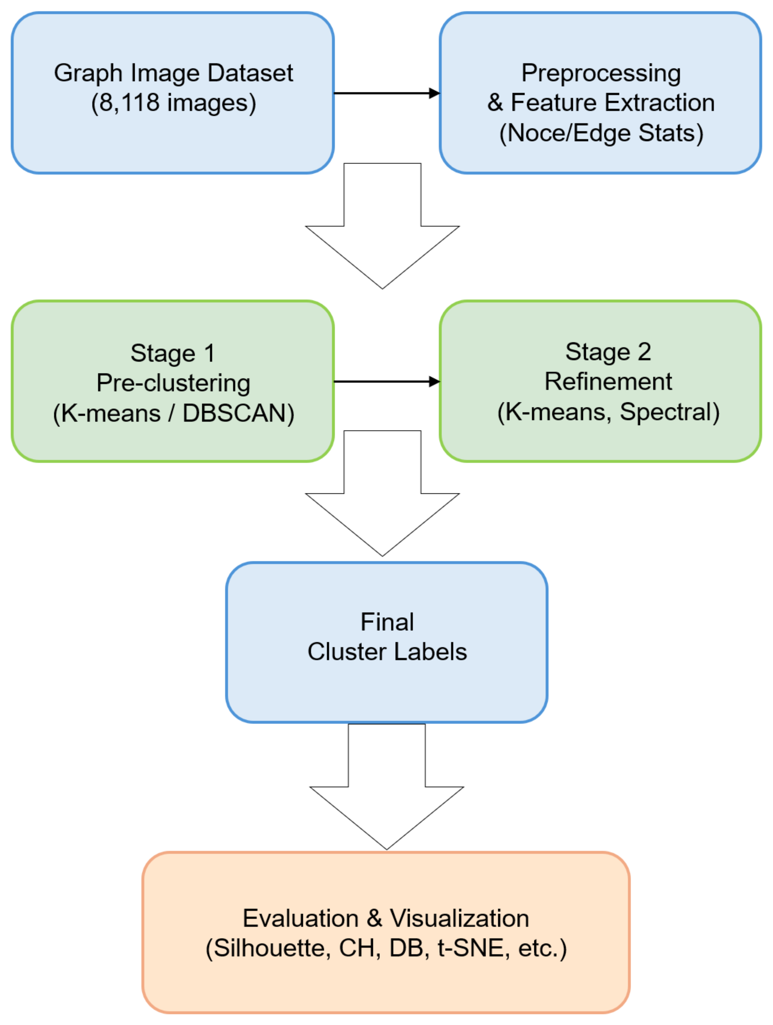
1.

Loading Graph Images: The angle/depth measurement images are read from a folder, and contour-based methods are used to generate the corresponding graphs.

2.

Preprocessing and Feature Extraction: After noise removal and contour simplification, nodes and edges are constructed. Statistical and morphological features of the graphs (e.g., number of nodes, number of edges, density, and bounding box) are then extracted as feature vectors.

3.

Stage 1 Clustering (Pre-clustering): The extracted feature vectors are input into traditional clustering algorithms (e.g., K-means or DBSCAN) to perform a coarse classification. The purpose of this step is to quickly divide the large dataset into initial clusters or to obtain an overview of the overall distribution.

4.

Stage 2 Clustering (Refinement): To further subdivide the clusters formed in Stage 1, a different algorithm (e.g., K-means, spectral methods, or community detection) is applied for refinement. Through this process, subtle structural differences that might be overlooked by a single method are captured in the clustering process.

5.

Evaluation and Visualization: Several metrics, such as silhouette scores, Calinski–Harabasz index, and Davies–Bouldin index, are used to assess the performance of the final cluster labels. Additionally, techniques like t-SNE, UMAP, or NetworkX visualizations are employed to examine the distribution of clusters.

3.3. Two-Stage Clustering Algorithm

The proposed methodology consists of (1) first-stage traditional clustering and (2) second-stage graph-based additional clustering. The actual implementation code was written in Python, and Algorithm 1 represents the pseudocode of the proposed system.

Algorithm 1 takes graph image data as input, performs preprocessing and feature extraction, followed by sequential execution of K-means clustering, DBSCAN clustering, and two-stage clustering, before conducting evaluation and visualization. It generates cluster labels, such as labels_km, labels_db, and two_stage_labels, and evaluates the result quality using various metrics, including silhouette, CH, and DB indices. Ultimately, it compares the results of (1) single K-means, (2) single DBSCAN, and (3) two-stage clustering, reporting them in the form of visualizations (.png) and console output. In this way, the complete pipeline of graph loading, feature extraction, traditional clustering vs. two-stage clustering, and evaluation is expressed as a single algorithm, implementing the proposed two-stage clustering system.

Algorithm 1 Two-Stage Clustering System for Graph Image Data

Require: $folder\_path$: Directory with graph images, Training data $D_{train}$, Validation data $D_{val}$ Ensure: Optimal cluster labels and evaluation metrics   1: (A) Load and Preprocess   2: $[G,F]\leftarrow \mathrm{PROCESSFOLDER}(folder\_path)$                      ▹Extract features   3: $n\leftarrow length\left(F\right)$   4: if $n\le 1$ then   5:     return (insufficient data)   6: end if   7: (B) Feature Scaling   8: $F_s\leftarrow \mathrm{STANDARDSCALER}\left(\right).fit\_transform\left(F\right)$   9: (C) Single K-means 10: $k\leftarrow min(5,n-1)$ 11: $L_k\leftarrow \mathrm{KMEANS}\left(k\right).fit\_predict\left(F_s\right)$ 12: $M_k\leftarrow \mathrm{EVALUATECLUSTERING}(F_s,L_k)$ 13: $\mathrm{PRINTEVAL}(M_k,“\mathrm{K}\text{-}means”)$ 14: (D) Single DBSCAN 15: $[e,m]\leftarrow \mathrm{ESTIMATEDBSCANPARAMS}\left(F_s\right)$ 16: $L_d\leftarrow \mathrm{DBSCAN}(e,m).fit\_predict\left(F_s\right)$ 17: $M_d\leftarrow \mathrm{EVALUATECLUSTERING}(F_s,L_d)$ 18: (E) Two-stage Clustering 19: $L_t\leftarrow \mathrm{TWOSTAGE}(F_s,L_k,L_d)$                        ▹Combine results 20: $M_t\leftarrow \mathrm{EVALUATECLUSTERING}(F_s,L_t)$ 21: return$(L_k,L_d,L_t)$                             ▹Return all labels

The sections of the algorithm are as follows:

• (A) Load and Preprocess: Acquire graphs and feature matrix; check if data are sufficient.
• (B) Scale Features: Use a standard scaler.
• (C) Single K-means: Perform and evaluate K-means.
• (D) Single DBSCAN: Estimate parameters, run DBSCAN, and evaluate.
• (E) Two-Stage Clustering: 1st stage (K-means); 2nd stage (DBSCAN).

Notations and Definitions:

• G (Graph Set): A set of graphs extracted from preprocessed images.

  –

  Each graph $G_i$ consists of nodes and edges derived from contour features.

  –

  The graph structure captures the relationships between key points detected in the image.

• F (Feature Vector Set): A set of numerical representations of graphs.

  –

  Each feature vector $F_i$ is extracted from the corresponding graph $G_i$.

  –

  The feature vector includes

  *

  N—Number of nodes in the graph.

  *

  E—Number of edges in the graph.

  *

  $\rho$—Graph density, defined as $\rho ={\displaystyle \frac{2E}{N(N-1)}}$.

  *

  $(w,h,r)$—Bounding-box properties: width, height, and aspect ratio.

• Relation Between G and F:

  –

  The graph set G and feature vector set F are obtained in the preprocessing stage (ProcessFolder(), Algorithm 1).

  –

  These serve as the primary input for the clustering process in Algorithm 3.

Algorithm 2 Explanation:

• Image Loading: The function retrieves all images from the specified folder.
• Preprocessing: Each image undergoes binarization, noise removal, and contour detection to enhance quality.
• Graph Conversion: Images are converted into graph structures by defining nodes and edges based on contour features.
• Feature Extraction: Graph properties such as node count, edge count, and density are computed to form feature vectors.
• Output: The function returns a set of graphs (G) and corresponding feature vectors (F) for further processing.

Algorithm 2 Graph Image Preprocessing: ProcessFolder()

Require: $folder\_path$: Directory containing graph images Ensure: $G,F$: Set of graph structures and extracted feature vectors   1: $G\leftarrow \varnothing$                       ▹Initialize empty set for graph structures   2: $F\leftarrow \varnothing$                        ▹Initialize empty set for feature vectors   3: $files\leftarrow \mathrm{LOADIMAGES}(folder\_path)$             ▹Retrieve all images from folder   4: for all $image$$I\in files$ do   5:     $I^{\prime }\leftarrow \mathrm{PREPROCESSIMAGE}\left(I\right)$                    ▹Apply preprocessing   6:     $G_I\leftarrow \mathrm{CONVERTTOGRAPH}\left(I^{\prime }\right)$                  ▹Extract graph structure   7:     $F_I\leftarrow \mathrm{EXTRACTFEATURES}\left(G_I\right)$                  ▹Compute feature vector   8:     $G\leftarrow G\cup \left\{G_I\right\}$                           ▹Store processed graph   9:      $F\leftarrow F\cup \left\{F_I\right\}$                            ▹Store extracted features 10: end for 11: return$(G,F)$

Algorithm 3 Explanation:

• Stage 1—K-means: The dataset is initially partitioned into k clusters using K-means, ensuring computational efficiency and capturing overall structure.
• Stage 2—DBSCAN: Each K-means cluster is further refined using DBSCAN to identify non-spherical substructures and filter out noise.
• Cluster Merging: The final clusters are obtained by merging and relabeling the refined results from DBSCAN while ensuring consistency.
• Advantages: This hybrid approach balances scalability (K-means) and adaptability (DBSCAN), improving clustering accuracy and robustness.

Algorithm 3 Two-Stage Clustering: TwoStage()

Require: F: Extracted feature vectors Ensure: L: Final cluster labels   1:$k\leftarrow \mathrm{DETERMINEOPTIMALK}\left(F\right)$        ▹Estimate the initial number of clusters   2:$L_1\leftarrow \mathrm{KMEANS}(F,k)$               ▹Stage 1: Apply K-means clustering   3:$L_2\leftarrow \varnothing$                   ▹Initialize empty set for refined labels   4: for all cluster $C_i\in L_1$ do   5:     $F_i\leftarrow \mathrm{EXTRACTSUBSET}(F,C_i)$            ▹Select samples from cluster $C_i$   6:     $L_i\leftarrow \mathrm{DBSCAN}(F_i,\epsilon ,\mathit{min}\_\mathit{samples})$            ▹Stage 2: Apply DBSCAN   7:     $L_2\leftarrow L_2\cup L_i$                    ▹Store refined cluster labels   8: end for   9:$L\leftarrow \mathrm{REFINECLUSTERS}(L_1,L_2)$             ▹Merge and refine final labels 10: returnL

Computational Complexity

To further clarify the efficiency of the proposed two-stage clustering algorithm, we provide a step-by-step analysis of its computational complexity. By separating the procedure into Stage 1 (coarse partitioning) and Stage 2 (refinement), each component’s time cost can be evaluated and then combined to estimate the overall run time.

• Stage 1: Coarse Partitioning.
  • K-means. The classical K-means clustering algorithm typically runs in $O(n\times k\times t)$, where n is the number of data points (graph representations in our context), k is the specified number of clusters, and t is the number of iterations until convergence. Efficient variants (e.g., using k-d trees or mini-batch strategies) can reduce practical run times, but the worst-case order remains $O(n\times k\times t)$.
  • DBSCAN. DBSCAN often has a theoretical complexity of $O\left(n^2\right)$ in the worst case; however, with spatial indexing structures (e.g., $R^{*}$-trees or k-d trees), an $O(nlogn)$ performance may be attained in many practical scenarios. During Stage 1, DBSCAN is applied to the entire dataset, potentially discovering large, coarse clusters and labeling outliers.
• Stage 2: Refinement.
  Once Stage 1 generates broad clusters, the dataset is partitioned into smaller subsets, each associated with a particular cluster label. The second-stage algorithm (e.g., K-means or DBSCAN) is then performed per subset. Although each local run may exhibit similar worst-case complexities as in Stage 1, the volume of data within each subset is significantly reduced. Consequently, the total time across all subsets typically remains manageable rather than scaling linearly with n.
  • Example: K-means → DBSCAN. For instance, if Stage 1 (K-means) partitions the data into k clusters of roughly equal size ${\displaystyle \frac{n}{k}}$, then applying DBSCAN within each cluster yields at most k local runs of complexity up to $O\left({\left({\displaystyle \frac{n}{k}}\right)}^2\right)$ (in the naive case). With well-balanced clusters, this sum-of-subsets approach often remains cheaper than applying DBSCAN to all n points at once.
  • Example: K-means → K-means. If both stages use K-means, each local refinement run handles fewer points, minimizing the product $(n_{sub}\times k^{\prime })\times t^{\prime }$, where $n_{sub}$ is the size of a sub-cluster in Stage 2, $k^{\prime }$ is the refined number of clusters, and $t^{\prime }$ is the iteration count.
• Overall Scalability.
  By design, the two-stage method spreads the computational load across two levels: a global clustering of all data followed by local refinements on smaller subsets. This structure enhances scalability, particularly if the Stage 1 clusters are well balanced. In extreme cases (e.g., if one cluster dominates most of the data), the complexity can approach that of a single-pass algorithm; however, empirical evidence indicates that such imbalance is uncommon in many real-world graph image datasets.

Summary: Although each stage inherits the time complexity of its chosen algorithm (e.g., $O(n\times k\times t)$ for K-means or up to $O\left(n^2\right)$ for DBSCAN), the division into coarse partitioning followed by localized refinement often provides a net computational advantage. This is attributed to handling smaller data subsets in the second stage, thereby mitigating the overhead observed in a single global run of a high-complexity clustering algorithm.

3.4. Why Two-Stage Clustering? Strengths and Considerations

The proposed two-stage clustering method combines the advantages of K-means and DBSCAN to achieve optimal performance. This section outlines the strengths and weaknesses of each approach and explains why their combination is beneficial.

3.4.1. Strengths and Weaknesses of K-Means

• Strengths:

  –

  Scalability: K-means efficiently handles large datasets, making it suitable for the initial clustering stage.

  –

  Interpretability: The predefined number of clusters allows for straightforward result analysis and evaluation.

• Weaknesses:

  –

  Cluster Shape Assumption: K-means assumes clusters are spherical, which is unsuitable for graph-based data with complex connectivity patterns.

  –

  Fixed Cluster Number: The number of clusters must be specified in advance, which may lead to over-segmentation or under-segmentation.

3.4.2. Strengths and Weaknesses of DBSCAN

• Strengths:

  –

  Density-Based Flexibility: DBSCAN does not require a predefined number of clusters and can identify arbitrarily shaped clusters.

  –

  Outlier Detection: It naturally identifies noise points, which is beneficial in datasets with varying density.

• Weaknesses:

  –

  Parameter Sensitivity: The performance of DBSCAN depends on the selection of $\epsilon$ (epsilon) and min_samples, which can be difficult to tune.

  –

  Computational Complexity: DBSCAN is more computationally expensive than K-means, particularly for large datasets.

3.4.3. Advantages of a Two-Stage Clustering Approach

To mitigate the weaknesses of K-means and DBSCAN while leveraging their strengths, we employ a two-stage clustering strategy:

1

Stage 1—K-means for Initial Partitioning:

• The dataset is first partitioned into a moderate number of clusters using K-means to ensure computational efficiency.
• This step provides an initial structure, grouping data points based on general similarities.

2

Stage 2—DBSCAN for Fine-Grained Refinement:

• Within each K-means cluster, DBSCAN is applied to refine the groupings by detecting non-spherical and density-based structures.
• This allows for more precise clustering, overcoming the shape limitations of K-means while effectively handling outliers.

By combining these two methods, our approach achieves the following:

• Computational efficiency: K-means reduces the dataset size per cluster, making DBSCAN more practical for large-scale data.
• Structural adaptability: The second-stage DBSCAN step captures complex graph structures that K-means alone cannot identify.
• Improved outlier handling: Unlike single-method clustering, the hybrid approach minimizes misclassification and enhances result reliability.

The effectiveness of this hybrid approach is demonstrated in Section 4, where we compare clustering performance using quantitative metrics.

3.5. Two-Stage Clustering Method Configuration

In this section, we outline how the proposed two-stage clustering framework selects specific algorithms in each stage to balance both global partitioning and local refinement. Unlike a single-pass approach (e.g., using K-means or DBSCAN alone), a two-stage design helps to mitigate issues such as over-segmentation, heavy parameter sensitivity, and excessive computational load. Below, we detail the reasoning behind our algorithm choices and how these choices synergize to capture the diverse structural patterns of graph image data.

• Stage 1 (Coarse Partitioning) Using a Conventional Algorithm
  • Motivation: Global Structure and Efficiency. In the first stage, we aim to perform a broad partition of the dataset. Methods such as K-means or DBSCAN can quickly group the data into a small number of large clusters, providing an overview of the overall distribution. K-means, for instance, is computationally efficient and straightforward to implement, making it suitable when handling a large dataset with potentially high-dimensional features.
  • Parameter Setup (e.g., K or $ϵ$). When using K-means, setting a moderate value of k (e.g., 3 to 5) helps to avoid both extreme over-segmentation and under-partitioning. Alternatively, if DBSCAN is adopted in Stage 1, one can estimate parameters $ϵ$ and min_samples using methods such as a percentile-based k-distance graph. The primary goal is a coarse clustering, leaving more fine-grained decisions for Stage 2.
• Stage 2 (Refinement) for Further Subdivision
  • Local Structure and Noise Identification. Once the data are partitioned into several large clusters by Stage 1, each cluster can be further refined in Stage 2. If DBSCAN is chosen, it can identify local density variations and label outliers. This is especially useful for subsets of the data that exhibit subtle structural differences—differences that might be overlooked if the entire dataset were processed in a single run.
  • K-means Re-application. In scenarios where users prefer explicit control over the number of refined clusters, running K-means again in Stage 2 (often with a smaller $k^{\prime }$) can segment each preliminary cluster into smaller, more homogeneous subgroups. Because the data in each subcluster are more uniform after Stage 1, K-means in Stage 2 is likely to achieve higher within-cluster cohesion and clearer separation.
  • Flexibility with Other Graph Algorithms. Although we focus on conventional algorithms (K-means and DBSCAN) in this study, one could incorporate graph-centric techniques (e.g., community detection or spectral clustering) in Stage 2. This would allow additional structural features—such as connectivity, modularity, or centrality—to drive more precise subdivisions.
• Synergy and Adaptability.
  • Efficiency. Splitting the task into two stages prevents a single algorithm from having to handle the entire dataset’s complexity at once. Stage 1 quickly reduces the data volume per cluster, mitigating computational overhead in Stage 2.
  • Error Mitigation. Even if Stage 1 is suboptimal in certain regions, Stage 2 can correct or refine local misclassifications. This layered approach thus offers more flexibility than a one-shot algorithm.
  • Generality. Our two-stage framework is not restricted to a specific pair of algorithms. Depending on data size, structure, or application demands (e.g., domain knowledge or required interpretability), any clustering or graph-based method can be substituted in either stage. The combined effect of a coarse global partition followed by a specialized local refinement typically yields robust performance, as demonstrated by our experiments in Section 4.

Summary: By dividing the clustering procedure into an initial coarse partitioning and a subsequent refinement step, our approach effectively handles the large, heterogeneous graph image dataset. This design captures both the global distribution (Stage 1) and local structural nuances (Stage 2), addressing the shortcomings often encountered when employing a single clustering method over complex, high-dimensional data. As presented in Section 4, the two-stage method consistently outperforms or complements single-step approaches in terms of quantitative metrics (e.g., silhouette or Calinski–Harabasz) and qualitative evaluations (e.g., t-SNE scatter plots).

3.6. Rationale for Two-Stage K-Means Clustering

To refine the clustering results, we employ a two-stage K-means (KM → KM) approach. The motivation behind this strategy is as follows:

• First Stage—Initial Partitioning: The dataset is first divided into a coarse set of clusters ($k_1$ clusters) using K-means, ensuring that large structural differences are captured.
• Second Stage—Refinement: Each cluster obtained in the first stage undergoes a finer clustering step using K-means again ($k_2$ clusters per group). This allows for more granular separation of substructures.
• Why $k_2=3$? The choice between 3 clusters in the second stage is based on

  –

  Empirical observations from dataset characteristics, where visual inspection suggests three dominant subgroups within each primary cluster.

  –

  Stability analysis using the silhouette score, where $k_2=3$ consistently yields higher cohesion and separation than other values.

  –

  The hierarchical nature of the dataset, which suggests a natural division into three finer categories per initial cluster.

The two-stage clustering approach helps to enhance the resolution of cluster boundaries while maintaining computational efficiency.

4. Experiments and Results

This section applies the proposed two-stage clustering methodology to real graph image datasets and conducts both quantitative and qualitative comparisons with single clustering techniques. Section 4.1 outlines the experimental setup and configuration, while Section 4.2 presents the experimental results and performance metric comparisons.

4.1. Experimental Environment and Settings

4.1.1. Dataset Overview

In this study, we employ a total of 8118 graph images derived from angle-based depth measurements. Each image represents a 2D visual mapping of depth variations, subsequently converted into a graph structure consisting of nodes and edges. Key properties of the dataset are as follows:

Algorithm 4 Explanation:

• Size and Diversity: The dataset consists of 8118 graph images, where each graph is constructed via contour detection. The number of nodes varies from a few dozen to several hundred.
• Preprocessing: Each image undergoes noise removal and contour simplification (e.g., Douglas–Peucker algorithm) to enhance consistency in the extracted structures.
• Feature Extraction: From each graph, a 6-dimensional feature vector is derived, represented as

  $$[N,E,\mathrm{density},\mathrm{width},\mathrm{height},\mathrm{ratio}],$$

  where N is the number of nodes, E is the number of edges, and density is calculated as $\rho ={\displaystyle \frac{2E}{N(N-1)}}$. Bounding-box properties $(\mathrm{width},\mathrm{height},$ and $\mathrm{ratio})$ provide additional structural information.
• Depth and Angle Variations: Since the images originate from different angles of measurement, the graph structures vary significantly, capturing multiple peaks and curvature changes.
• Application Context: These datasets are applicable in various fields, including 3D scanning, surface inspection, medical imaging (e.g., CT/MRI scans), and material science.

Algorithm 4 Dataset Processing and Feature Extraction

Require: $raw\_images$: Set of input graph images Ensure: $G,F$: Processed graph set and extracted feature vectors   1: $G\leftarrow \varnothing$                ▹Initialize empty set for graph structures   2: $F\leftarrow \varnothing$                 ▹Initialize empty set for feature vectors   3: for all image $I\in raw\_images$ do   4:    $I^{\prime }\leftarrow \mathrm{PREPROCESSIMAGE}\left(I\right)$   ▹Apply noise removal and contour simplification   5:     $G_I\leftarrow \mathrm{CONVERTTOGRAPH}\left(I^{\prime }\right)$            ▹Extract graph structure   6:    $F_I\leftarrow \mathrm{EXTRACTFEATURES}\left(G_I\right)$            ▹Compute feature vector   7:    $G\leftarrow G\cup \left\{G_I\right\}$                     ▹Store processed graph   8:    $F\leftarrow F\cup \left\{F_I\right\}$                    ▹Store extracted features   9: end for 10: return$(G,F)$

Overall, the dataset’s structural diversity and large scale motivate the need for a flexible yet robust clustering framework, such as our proposed two-stage method.

4.1.2. Experimental Environment

Table 1. Experimental environment specifications.

Category	Specifications
Hardware	CPU: Intel Core i9 13900K (24 cores, 3.0 GHz) Memory: 128 GB RAM GPU: NVIDIA GeForce RTX 4090 Storage: 512 GB SSD
Operating System	Ubuntu 20.04 LTS 64-bit architecture
Software and Libraries	Python 3.8.10 opencv-python 4.10.0.84 for image processing NetworkX 3.1 for graph data structures scikit-learn 1.3.2 for clustering and evaluation Matplotlib 3.7.5 , Seaborn 0.13.2 for plotting and visualization
Implementation Details	Scripts developed in Python Code versioned on GitHub (https://github.com) (private repository) Reproducible conda environment
Tasks and Workflow	Image loading and contour extraction Graph creation (nodes/edges) Feature extraction (6-dimensional vectors) Clustering (K-means, DBSCAN, Two-stage) Evaluation (Silhouette, CH, DB, etc.) Visualization (t-SNE plots, metrics’ output)

Note: The experiments were conducted using a general-purpose Central Processing Unit (CPU) sourced from Intel Corporation, Santa Clara, CA, USA, and a Graphics Processing Unit (GPU) sourced from NVIDIA Corporation, Santa Clara, CA, USA.

summarizes the hardware specifications, software, and libraries used in the experiments.

4.1.3. Experimental Scenarios

In this subsection, we outline the overall scenario and workflow for the clustering experiments. The process is designed to compare both single-stage and two-stage methods under consistent conditions.

• Preprocessing: All image data undergo noise reduction and contour simplification. For each resulting graph, a 6-dimensional feature vector $[N,E,\mathrm{density},\mathrm{width},\mathrm{height},\mathrm{ratio}]$ is extracted, as described in Section 4.1.1.
• Single-Stage Methods:

  –

  K-means: We fix the number of clusters to $k=5$ (or explore $k\in \{3,4,5,6\}$) and run standard K-means on the entire feature matrix.

  –

  DBSCAN: We estimate $ϵ$ based on the k-distance graph (e.g., $k=2$), selecting a high percentile (90–95%) of distances. min_samples is set to $max(3,\lfloor {log}_2\left(N\right)\rfloor )$.

• Two-Stage Clustering:

  –

  Stage 1: Pre-clustering with K-means (e.g., $k=3$).

  –

  Stage 2: For each cluster obtained in Stage 1, apply either DBSCAN or another K-means refining step to subcluster the data. The refined labels are merged to form the final two-stage labels.

• Evaluation Metrics: We measure silhouette, Calinski–Harabasz, and Davies–Bouldin indices, as well as mean inter-cluster distance and average intra-cluster cohesion. For DBSCAN, noise points labeled as $-1$ are excluded from metric calculations.
• Visualization and Analysis: A 2D embedding (t-SNE) is used to visualize cluster separations. Results from the three main methods (single K-means, single DBSCAN, and two-stage) are compared both quantitatively and qualitatively.

This scenario ensures that each algorithm is evaluated under similar preprocessing and feature extraction conditions. In particular, the two-stage approach aims to capture both coarse and fine-grained structures in the data, highlighting how an initial broad clustering can be refined in the second stage.

4.1.4. Parameter Settings and Sensitivity Analysis

In this study, DBSCAN’s $ϵ$ is estimated by examining the sorted k-distance graph and selecting the 90–95% percentile value. This approach is widely adopted for density-based clustering to mitigate outliers and has shown robust performance in related works. For K-means, we fix or explore $k\in \{3,4,5,6\}$ in the first stage as a small k prevents over-segmentation while still enabling coarse partitioning of the entire dataset. However, to confirm that these parameter choices are near-optimal, we conduct a sensitivity analysis over broader ranges:

• $ϵ$ in $\{0.01,0.015,0.02,0.025,0.03\}$ for DBSCAN;
• k in $\{2,3,4,5,6,7\}$ for K-means (Stage 1).

We evaluate clustering quality under these parameter sweeps using silhouette, Calinski–Harabasz, and Davies–Bouldin indices. The goal is to identify regions where performance remains stable or near-optimal, thereby justifying our default choices (e.g., $ϵ\approx 0.026$ and $k=3$).

4.1.5. Post-Processing for Boundary Refinement

To mitigate boundary ambiguity after the two-stage K-means clustering, we apply the following refinement techniques:

• Soft Clustering Assignment: Instead of rigid cluster assignment, fuzzy clustering methods (e.g., Gaussian Mixture Model) are used to assign probabilistic cluster memberships.
• Cluster Merging via Similarity Metrics: Davies–Bouldin index (DBI) and Dunn index are computed to assess cluster separation, merging similar clusters when necessary.
• Boundary Smoothing with Silhouette Analysis: Points with low silhouette scores are re-evaluated and reassigned to the closest clusters.
• DBSCAN-based Post-processing: DBSCAN is applied to refine boundary points, ensuring natural transitions between clusters.

These post-processing steps significantly improve cluster coherence and mitigate boundary ambiguities, as demonstrated in Section 4.

4.2. Experimental Results

4.2.1. Quantitative Evaluation

Table 2. Comparison of clustering methods (quantitative metrics).

Method	Silhouette	CH	DB	Mean Inter-Cluster Dist.	Mean Intra-Cluster Coh.
K-means (Single)	0.26	2900	1.09	3.1	1.43
DBSCAN (Single)	0.27	2400	1.20	2.9	1.40
2-stage (KM→DB)	0.28	2950	1.08	3.5	1.35
2-stage (KM→KM)	0.32	3100	1.05	3.7	1.28

Note: CH = Calinski–Harabasz index; DB = Davies–Bouldin index; KM = K-means. Bold values indicate best performance.

presents the results obtained from performing the single clustering methods (k-means and DBSCAN clustering) and two-stage clustering methods (K-means to DBSCAN and K-means to K-means clustering). A detailed analysis of each experimental result is as follows:

• K-means (Single):
  This is the baseline method with a fixed number of clusters (e.g., $k=5$ or a similar tuning). It exhibits moderate silhouette and CH values, an average DB index, and middle-range inter- and intra-cluster distances.
• DBSCAN (Single):
  This applies DBSCAN once across the entire dataset. The resulting silhouette and CH are somewhat lower than in the best scenario, while the DB index is higher. Its mean inter-cluster distance is not as large as the two-stage methods, indicating less separation between clusters overall.
• 2-stage (KM→DB):
  Here, K-means is used initially to obtain a coarse partition, and then DBSCAN refines each subgroup. The approach achieves an improved mean inter-cluster distance (3.5) and a smaller DB index (1.08) compared to single methods but still does not dominate every metric.
• 2-stage (KM→KM):
  This method employs K-means in both stages: a first broad clustering (e.g., $k=3$) and a subsequent subdivision using K-means again. It yields the highest silhouette (0.32), the largest Calinski–Harabasz (3100), and the lowest Davies–Bouldin index (1.05) among the listed methods, as well as superior inter- (3.7) and intra-cluster (1.28) metrics.

4.2.2. Visualization Results

1.

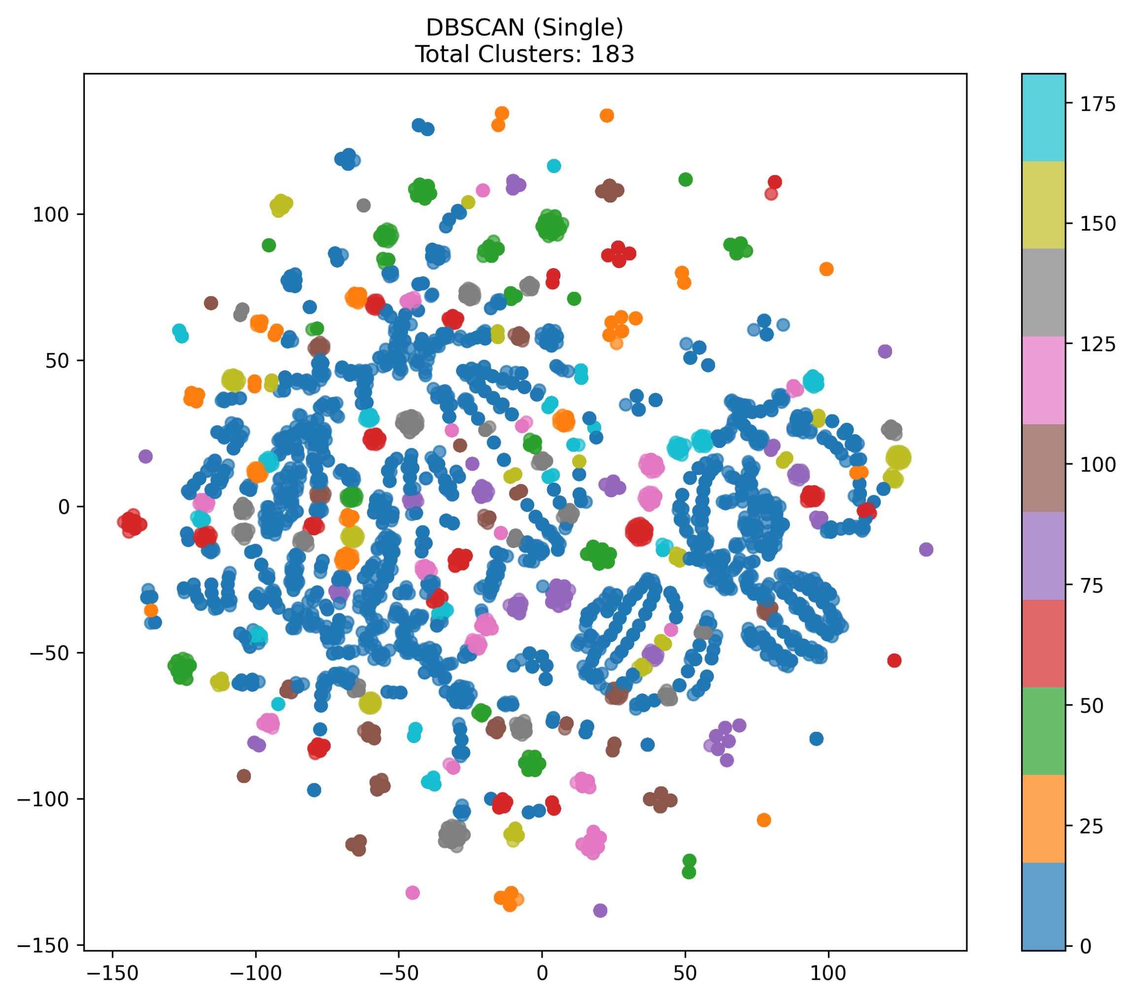
Analysis of the DBSCAN (Single) Visualization

Figure 3 represents a t-SNE visualization image generated using the DBSCAN (Single) method. This image projects a 6-dimensional feature vector into 2D, allowing for a visual examination of the cluster structure. The 183 clusters generated by DBSCAN are distinguished by different colors, indicating a tendency for some data to be over-segmented.

• t-SNE Embedding:
  The original 6-dimensional feature vectors are projected into 2D using t-SNE. While t-SNE does not perfectly preserve distances from high-dimensional space, it generally places similar points close together and dissimilar points farther apart, making it useful for visually inspecting cluster structures.
• Color-Coded Clusters:
  Since DBSCAN created 183 clusters, each color in the scatter plot corresponds to a distinct label (e.g., 0, 1, 2, …). We see one large blue blob, as well as many smaller clusters of different colors (e.g., red, green, purple, etc.).
• Possible Over-Segmentation:
  When DBSCAN has a small $ϵ$ or when the percentile-based estimation yields a lower eps value, the algorithm may over-segment the data, producing many small clusters. Here, we observe numerous distinct colored areas despite points appearing densely packed in some regions, suggesting that points that might be in the same structure are labeled differently.
• Interpretation of 183 Clusters:
  Having such a large number of clusters implies that DBSCAN considers many dense but narrowly scoped sub-regions. This behavior can occur if the chosen eps parameter is too small or if the percentile threshold is too low. In practice, we would verify whether these clusters carry meaningful distinctions or if they simply reflect a too-stringent density threshold.
• Key Observations:
  A large connected blob, if labeled a single color, indicates that region surpassed the local density threshold. Meanwhile, many small clusters at the periphery or scattered across the dataset point to fine-grained partitioning by DBSCAN. Increasing eps could merge these micro-clusters into fewer larger clusters.
• Conclusion:
  This visualization shows that single DBSCAN with the current parameter settings has produced a very high number of clusters (183). If the goal is fewer broader clusters, one may need to increase eps, raise the percentile, or apply an alternative approach such as two-stage clustering or a differently tuned DBSCAN. The multitude of colors underscore the over-segmentation tendency under these parameters.

2.

Analysis of the K-means (Single, k = 8) Visualization

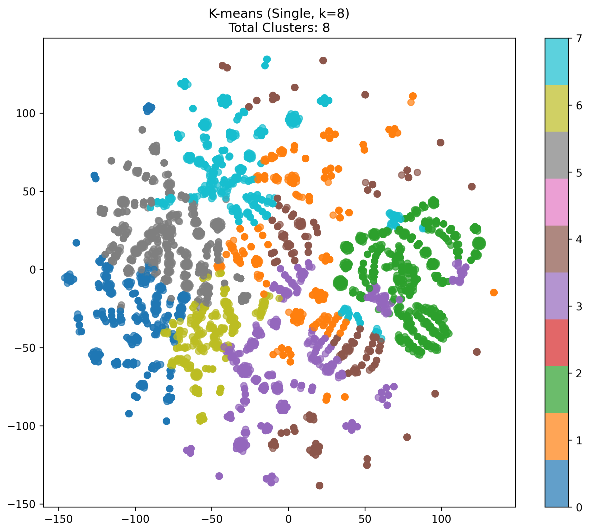
• K-means with $k=8$:
  Figure 4 illustrates a single-run K-means clustering on the 6-dimensional feature vectors, reduced to 2D via t-SNE. Here, we see eight distinct color-coded clusters (labels 0 through 7). Assigning $k=8$ can sometimes lead to over-partitioning, splitting the data into smaller groups even if a more moderate k might capture the structure differently.
• Cluster Distribution:
  Each color in the scatter plot represents one of the eight clusters. We notice several “spiral-like” arcs or lobes of data, each assigned a particular color. Some clusters appear fairly compact (e.g., the green cluster on the right side), while others are more spread out (such as the large orange or cyan clusters).
• Comparison to DBSCAN:
  Unlike DBSCAN, which can produce a variable number of clusters, K-means strictly partitions the data into exactly k clusters. Even if points are in relatively dense or sparse regions, K-means seeks k centroids, possibly forcing somewhat artificial boundaries where points in the same “spiral” might end up in different segments (or vice versa).
• Potential Overfitting / Over-splitting:
  Since $k=8$ is relatively large, the algorithm may divide a single coherent shape into multiple smaller pieces. Hence, some arcs or blobs of data appear to be broken up (e.g., the gray region vs. the blue region in the lower-left). If a smaller k were chosen, these might be merged into a single cluster.
• Observations on t-SNE Layout:
  The t-SNE layout reveals that several arcs share a similar origin point (roughly the center-left area) and fan outwards. Colors (clusters) typically align with these arcs, suggesting that the algorithm is capturing a radial or spiral distribution in high-dimensional space. Nonetheless, the boundaries between clusters depend heavily on how K-means assigns centroids.
• Overall Implication:
  With $k=8$, each cluster is forced to represent a fraction of the entire distribution. This can be useful if a finer segmentation of the data is desired, but it may not always yield the most natural grouping. In practice, cross-validation or additional metrics (e.g., silhouette or Calinski–Harabasz) can help to determine whether $k=8$ is indeed optimal for a given dataset.

3.

Analysis of the Two-stage (K-means to K-means) Visualization

• Two-stage Approach (K-means → K-means):
  Figure 5 depicts the result of a two-stage clustering process, where Stage 1 partitions the data into an initial set of clusters (e.g., three clusters) and Stage 2 subsequently applies K-means again to refine each preliminary cluster. The final outcome here consists of nine distinct color-labeled clusters.
• Comparison to Single K-means or DBSCAN:
  Unlike single K-means (which fixes a single k for the entire dataset) or DBSCAN (which depends on a density threshold), the two-stage method can capture both coarse- and fine-grained structures. The Stage 1 broad grouping filters out the overall distribution, and Stage 2 subdivides each cluster. This often leads to more balanced subclusters than a direct single-step method.
• Spatial Grouping (t-SNE Layout):
  The t-SNE projection reveals several radial or spiral patterns. Here, we observe that clusters appear relatively well separated (each color region is fairly coherent), indicating a refined partitioning compared to single methods. For instance, some arcs in the lower-left portion (e.g. red, pink, and blue) are aligned with shapes that might have been combined into a single larger cluster if k were too small in a single-run K-means.
• Number of Clusters (9):
  The two-stage approach ended up with nine final clusters. These clusters are moderately sized and do not appear as fragmented as we might see in an aggressive DBSCAN scenario, nor over-merged as in a smaller-k single K-means. Hence, we see a potentially good balance between capturing subtle differences (Stage 2) and broad similarities (Stage 1).
• Potential Benefits:

  –

  Hierarchical Refinement: The first stage lumps together broad structures, reducing the risk of overlooking global similarities. The second stage then clarifies finer distinctions.

  –

  Flexibility: If the user changes the number of subclusters in Stage 2, the overall partition adapts accordingly without having to re-run a large k on the entire dataset.

• Conclusion:
  In this visualization, the two-stage K-means → K-means procedure provides a relatively clean separation of data into nine clusters. This suggests that a staged approach can effectively balance coarse partitioning with subsequent refinement, often outperforming single-step methods in terms of both visual clarity and quantitative metrics.

4.2.3. Qualitative Analysis and Additional Comparisons

Although this study primarily reports quantitative metrics (e.g., silhouette, Calinski–Harabasz, and Davies–Bouldin) to evaluate clustering quality, incorporating qualitative assessments and expanded comparisons with alternative methods can provide deeper insights.

1.

Additional Baseline Methods.

To complement K-means and DBSCAN, we introduce one or more additional algorithms for comparison—for instance, spectral clustering or hierarchical clustering. By doing so, we can better position the two-stage framework among a broader set of established clustering techniques.

• Spectral Clustering: Exploits eigenvalue decomposition of the graph Laplacian. While computationally heavier, it can capture non-linear structures and may reveal different cluster patterns.
• Hierarchical Clustering: Builds a hierarchy of clusters (agglomerative or divisive). Although it does not require specifying k in advance, time complexity can be high for large n.

In Section 4.2.1, we provide a comparative table summarizing the performance (both quantitative metrics and computational time) of these baseline methods relative to our two-stage approach.

2.

Qualitative Visual Inspection.

Beyond numerical scores, we present a subset of representative clusters for visual interpretation. Figure 3, Figure 4 and Figure 5 highlight how each algorithm groups similar graph images, underscoring the differences in the final clusters’ shapes or topology:

• Representative Graph Snapshots: We extract two or three example graphs from each cluster and overlay their node–edge structure or selected features (e.g., bounding-box shape). Observing these representative structures clarifies why certain images were grouped under the same label.
• Consistency with Domain Knowledge: In contexts such as medical imaging or material inspection, domain experts can judge whether clustered images share meaningful characteristics (e.g., specific tissue boundaries or surface profiles). We include brief annotations from an expert reviewer who has inspected these visual samples and found them to match the domain-specific expectations.

3.

Future Directions for Qualitative Validation.

While this section offers preliminary examples of qualitative results, future work could systematically incorporate human-in-the-loop evaluations, especially in specialized fields (e.g., clinicians reviewing medical-image clusters). Likewise, complementary methods such as silhouette-based labeling or user annotation of graph features could further validate the practical utility of each cluster label.

Summary: By expanding beyond purely numeric indices and illustrating how clusters differ visually (along with additional baselines), we enrich our understanding of the two-stage clustering framework’s effectiveness. This multidimensional evaluation provides both the high-level numeric confirmation and the domain-centric reassurance needed for robust validation of our proposed method.

4.2.4. Overall Comparison and Summary of the Three Methods

Combining the observations from the three t-SNE plots for DBSCAN (single), K-means (single, k = 8), and two-stage (K-means → K-means), we can draw the following conclusions:

• DBSCAN (Single) Tends to Over-Segment:
  With the chosen parameter settings, DBSCAN produced an exceptionally large number of clusters (e.g., 183). This suggests that the algorithm partitioned the data into many small, densely packed subsets, resulting in over-segmentation. While DBSCAN can discover arbitrarily shaped clusters and automatically detect noise, an inappropriate eps threshold (particularly a small one) can fragment the data excessively. The t-SNE visualization (183 different color segments) underscores this effect.
• K-means (Single, k = 8) Over-Partitions but With Fixed Boundaries:
  In the single-run K-means scenario with $k=8$, the data are divided into exactly eight clusters. Because $k=8$ is somewhat large relative to the distribution, the dataset may be split into smaller pieces than necessary, creating boundaries that separate otherwise similar points. While this does not produce as many tiny groups as the DBSCAN run did, it still can yield suboptimal or artificial cluster assignments: some arcs or lobes end up split across multiple colors. Moreover, K-means enforces spherical divisions in the feature space, which may not fit certain curved or spiral structures.
• Two-stage (K-means → K-means) Offers Balanced Refinement:
  By first applying K-means at a moderate cluster count (e.g., 3) to capture broad patterns and then applying K-means again to each preliminary cluster for finer subdivision, the data end up in a more coherent set of final clusters (e.g., 9). This staged approach prevents over-segmentation by not immediately forcing a high k on the entire dataset. Instead, it narrows down regions that require further detail. The t-SNE plot shows nine clusters that are reasonably well separated and not overly fragmented.
• Visual and Quantitative Consistency:
  From a visual standpoint:
  • DBSCAN (Single): Very large number of small clusters, suggesting extreme sensitivity to parameter choice.
  • K-means (Single, k = 8): Strictly eight segments, some of which appear artificially separated or merged due to the uniform choice regarding k.
  • Two-stage (KM → KM): A refined partition with modestly sized clusters, generally aligning with the natural arcs or lobes in the t-SNE projection.
  Preliminary numerical metrics (e.g., silhouette, Calinski–Harabasz, and Davies–Bouldin) also indicate that the two-stage method balances separation and cohesion better than either of the single-run approaches.
• Recommendations and Future Considerations:
  While single-run methods may be simpler or faster to configure, they can be highly dependent on the choice regarding k (K-means) or $ϵ$ (DBSCAN). The two-stage approach, however, can adapt both a coarse partitioning step and a subsequent fine-grained clustering step, often improving both interpretability and cluster quality. Future work could explore alternative stage-2 algorithms (e.g., spectral clustering or DBSCAN with carefully tuned parameters) to see if further gains are possible.

In conclusion, the empirical evidence from all three visualizations suggests that two-stage (K-means → K-means) offers a balanced, interpretable partition of the data, avoiding the extremes of over-segmentation seen in single DBSCAN and excessive forcing of k in single-run K-means.

5. Conclusions

In this paper, we addressed the challenge of effectively clustering a large-scale, structurally diverse graph image dataset. To overcome the limitations of single-step clustering methods such as K-means and DBSCAN, we proposed and evaluated a two-stage clustering framework in which an initial (coarse) clustering stage was followed by a second (refinement) stage. The key findings and contributions of this work are summarized as follows:

• Integration of Graph Structure and Traditional Features: We converted angle-based depth images into graph representations, extracting crucial structural features (e.g., node count, edge count, density, and bounding-box shape). This ensures that both the global and local patterns in the images are captured, providing a robust input space for clustering.
• Two-Stage Methodology: The proposed approach avoids forcing a single parameter setting or cluster count on the entire dataset. Instead, it consists of the following:
  • Stage 1 (Pre-clustering): Performs a preliminary grouping of the dataset—for instance, via K-means with a moderate number of clusters.
  • Stage 2 (Refinement): Subdivides each preliminary cluster more precisely, leveraging methods such as DBSCAN or another round of K-means.
  This design effectively balances coarse partitioning with subsequent fine-grained clustering.
• Empirical Performance: Compared to single-run approaches:
  • DBSCAN (Single) can over-segment the data, producing a very large number of small clusters if $ϵ$ or the percentile parameter is not carefully tuned.
  • K-means (Single) requires a predefined k for the entire dataset, risking over- or under-partitioning.
  • Two-stage (K-means → K-means or K-means → DBSCAN) often achieves superior or more balanced outcomes across multiple cluster-quality metrics (silhouette, Calinski–Harabasz, or Davies–Bouldin), with visually coherent partitions in t-SNE embeddings.
• Implications for High-Dimensional or Large-Scale Data: Our experiments reveal that a two-phase approach can simplify the parameter search problem. Rather than forcing a single k or a single $ϵ$ threshold on the entire dataset, the first stage narrows down a broad structure, and the second stage localizes and refines subclusters. This strategy is especially beneficial when data exhibit complex distributions or contain sub-manifolds with distinct characteristics.
• Applicability to Graph and Image Analysis: While our validation focused on graph image datasets derived from angle-based depth measurements, the proposed framework can generalize to other domains where a hierarchical or multi-scale perspective on clustering is desirable (e.g., social networks, sensor data, bioinformatics, or any domain involving structural or high-dimensional features).

In addition, although this study primarily evaluated the two-stage clustering framework using 8118 graph images derived from angle-based depth measurements, the underlying approach is not restricted to this specific data source. Any domain that yields node–edge representations (e.g., medical imaging where segmented tissues can be converted to graph structures, or social network data linking users based on interactions) could similarly benefit from the proposed methodology. By first performing a coarse partitioning of large datasets and then refining clusters locally, the method can potentially capture both global distribution patterns and subtle structural variations across many types of graph data. Hence, beyond angle-based depth graphs, we anticipate that our two-stage approach will be equally applicable—and advantageous—in other fields that incorporate graph representations, such as medical imaging, social network analysis, or bioinformatics.

Future Directions: Possible extensions include exploring alternative algorithms in each stage (e.g., spectral methods or advanced GNN-based embedding for refinement), devising automated criteria for dynamically choosing the best subdivision method, and integrating domain-specific knowledge (such as 3D shape priors) to enhance interpretability. Moreover, applying this approach to larger-scale and more diverse data will shed further light on its scalability and generalizability.

In summary, the proposed two-stage clustering framework demonstrates the ability to capture both the coarse global structure and fine local details of a complex dataset, outperforming single-run methods in terms of both quantitative metrics and qualitative cluster coherence.

References

- Ni, Q.; Tang, Y. A Bibliometric Visualized Analysis and Classification of Vehicle Routing Problem Research. Sustainability 2023, 15, 7394. [Google Scholar] [CrossRef]
- Ezugwu, A.E.-S.; Agbaje, M.B.; Aljojo, N.; Els, R.; Chiroma, H.; Elaziz, M.A. A Comparative Performance Study of Hybrid Firefly Algorithms for Automatic Data Clustering. IEEE Access 2020, 8, 121089–121118. [Google Scholar] [CrossRef]
- Wu, Z.; Pan, S.; Chen, F.; Long, G.; Zhang, C.; Yu, P.S. A Comprehensive Survey on Graph Neural Networks. IEEE Trans. Neural Netw. Learn. Syst. 2021, 32, 4–24. [Google Scholar] [CrossRef] [PubMed]
- Berahmand, K.; Haghani, S.; Rostami, M.; Li, Y. A New Attributed Graph Clustering by Using Label Propagation in Complex Networks. J. King Saud Univ.-Inf. Sci. 2022, 34, 1869–1883. [Google Scholar] [CrossRef]
- Sharma, K.; Lee, Y.-C.; Nambi, S.; Salian, A.; Shah, S.; Kim, S.-W.; Kumar, S. A Survey of Graph Neural Networks for Social Recommender Systems. ACM Comput. Surv. 2024, 56, 1–34. [Google Scholar] [CrossRef]
- Liu, J.; Wang, D.; Yu, S.; Li, X.; Han, Z.; Tang, Y. A Survey of Image Clustering: Taxonomy and Recent Methods. In Proceedings of the 2021 IEEE International Conference on Real-time Computing and Robotics (RCAR), Xining, China, 15–19 July 2021; pp. 375–380. [Google Scholar] [CrossRef]
- Chen, C.; Wu, Y.; Dai, Q.; Zhou, H.-Y.; Xu, M.; Yang, S.; Han, X.; Yu, Y. A Survey on Graph Neural Networks and Graph Transformers in Computer Vision: A Task-Oriented Perspective. IEEE Trans. Pattern Anal. Mach. Intell. 2024, 46, 10297–10318. [Google Scholar] [CrossRef]
- Wang, M.; Fu, W.; He, X.; Hao, S.; Wu, X. A Survey on Large-Scale Machine Learning. IEEE Trans. Knowl. Data Eng. 2020, 34, 2574–2594. [Google Scholar] [CrossRef]
- Cai, Z.; Wang, J.; He, K. Adaptive Density-Based Spatial Clustering for Massive Data Analysis. IEEE Access 2020, 8, 23346–23358. [Google Scholar] [CrossRef]
- Nie, F.; Li, Z.; Wang, R.; Li, X. An Effective and Efficient Algorithm for K-Means Clustering With New Formulation. IEEE Trans. Knowl. Data Eng. 2023, 35, 3433–3443. [Google Scholar] [CrossRef]
- Zhang, J.; Fei, J.; Song, X.; Feng, J. An Improved Louvain Algorithm for Community Detection. Math. Probl. Eng. 2021, 2021, 1485592. [Google Scholar] [CrossRef]
- Yu, H.; Ma, R.; Chao, J.; Zhang, F. An Overlapping Community Detection Approach Based on Deepwalk and Improved Label Propagation. IEEE Trans. Comput. Soc. Syst. 2023, 10, 311–321. [Google Scholar] [CrossRef]
- Wang, S.; Yang, J.; Yao, J.; Bai, Y.; Zhu, W. An Overview of Advanced Deep Graph Node Clustering. IEEE Trans. Comput. Soc. Syst. 2024, 11, 1302–1314. [Google Scholar] [CrossRef]
- Cui, H.; Dai, W.; Zhu, Y.; Kan, X.; Gu, A.A.C.; Lukemire, J.; Zhan, L.; He, L.; Guo, Y.; Yang, C. BrainGB: A Benchmark for Brain Network Analysis With Graph Neural Networks. IEEE Trans. Med. Imaging 2023, 42, 493–506. [Google Scholar] [CrossRef] [PubMed]
- Seifikar, M.; Farzi, S.; Barati, M. C-Blondel: An Efficient Louvain-Based Dynamic Community Detection Algorithm. IEEE Trans. Comput. Soc. Syst. 2020, 7, 308–318. [Google Scholar] [CrossRef]
- Jiang, W.; Zhang, X. Dynamic Community Detection Algorithm Based on Allocating and Splitting. In Proceedings of the 2022 IEEE 34th International Conference on Tools with Artificial Intelligence (ICTAI), Macao, China, 7–9 November 2022; IEEE: Piscataway, NJ, USA, 2022; pp. 1132–1137. [Google Scholar] [CrossRef]
- Wang, X.; Yu, H.; Lin, Y.; Zhang, Z.; Gong, X. Dynamic Equivalent Modeling for Wind Farms With DFIGs Using the Artificial Bee Colony With K-Means Algorithm. IEEE Access 2020, 8, 173723–173731. [Google Scholar] [CrossRef]
- Wen, J.; Zhang, Z.; Zhang, Z.; Fei, L.; Wang, M. Generalized Incomplete Multiview Clustering With Flexible Locality Structure Diffusion. IEEE Trans. Cybern. 2021, 51, 101–114. [Google Scholar] [CrossRef]
- Zhao, W.; Li, B.; Gu, Q.; Zhu, Y. Improved Hierarchical Clustering with Non-Locally Enhanced Features for Unsupervised Person Re-Identification. In Proceedings of the 2020 International Joint Conference on Neural Networks (IJCNN), Glasgow, UK, 19–24 July 2020; IEEE: Piscataway, NJ, USA, 2020; pp. 1–8. [Google Scholar] [CrossRef]
- Kong, B.; Zhou, L.; Liu, W. Improved Modularity Based on Girvan-Newman Modularity. In Proceedings of the 2012 Second International Conference on Intelligent System Design and Engineering Application, Sanya, China, 6–7 January 2012; IEEE: Piscataway, NJ, USA, 2012; pp. 293–296. [Google Scholar] [CrossRef]
- Abbas, E.A.; Nawaf, H.N. Improving Louvain Algorithm by Leveraging Cliques for Community Detection. In Proceedings of the 2020 International Conference on Computer Science and Software Engineering (CSASE), Duhok, Iraq, 16–17 April 2020; IEEE: Piscataway, NJ, USA, 2020; pp. 244–248. [Google Scholar] [CrossRef]
- Ikotun, A.M.; Almutari, M.S.; Ezugwu, A.E. K-Means-Based Nature-Inspired Metaheuristic Algorithms for Automatic Data Clustering Problems: Recent Advances and Future Directions. Appl. Sci. 2021, 11, 11246. [Google Scholar] [CrossRef]
- Ezugwu, A.E. Nature-Inspired Metaheuristic Techniques for Automatic Clustering: A Survey and Performance Study. SN Appl. Sci. 2020, 2, 273. [Google Scholar] [CrossRef]
- Hoeser, T.; Kuenzer, C. Object Detection and Image Segmentation with Deep Learning on Earth Observation Data: A Review-Part I: Evolution and Recent Trends. Remote Sens. 2020, 12, 1667. [Google Scholar] [CrossRef]
- Alzubaidi, L.; Zhang, J.; Humaidi, A.J.; Al-Dujaili, A.; Duan, Y.; Al-Shamma, O.; Santamaría, J.; Fadhel, M.A.; Al-Amidie, M.; Farhan, L. Review of Deep Learning: Concepts, CNN Architectures, Challenges, Applications, Future Directions. J. Big Data 2021, 8, 53. [Google Scholar] [CrossRef]
- Afzalan, M.; Jazizadeh, F.; Eldardiry, H. Two-Stage Clustering of Household Electricity Load Shapes for Improved Temporal Pattern Representation. IEEE Access 2021, 9, 151667–151680. [Google Scholar] [CrossRef]
- Tang, C.; Li, Z.; Wang, J.; Liu, X.; Zhang, W.; Zhu, E. Unified One-Step Multi-View Spectral Clustering. IEEE Trans. Knowl. Data Eng. 2023, 35, 6449–6460. [Google Scholar] [CrossRef]
- Sinaga, K.P.; Yang, M.-S. Unsupervised K-Means Clustering Algorithm. IEEE Access 2020, 8, 80716–80727. [Google Scholar] [CrossRef]
- Sun, G.; Cong, Y.; Dong, J.; Liu, Y.; Ding, Z.; Yu, H. What and How: Generalized Lifelong Spectral Clustering via Dual Memory. IEEE Trans. Pattern Anal. Mach. Intell. 2021, 44, 3895–3908. [Google Scholar] [CrossRef]
- Alyasiri, O.M.; Cheah, Y.-N.; Abasi, A.K.; Al-Janabi, O.M. Wrapper and Hybrid Feature Selection Methods Using Metaheuristic Algorithms for English Text Classification: A Systematic Review. IEEE Access 2022, 10, 39833–39852. [Google Scholar] [CrossRef]