Abstract
In semiconductor manufacturing, the final testing phase is critical for ensuring chip quality and operational efficiency. Accurate yield prediction at this stage optimizes testing workflows, boosts production efficiency, and enhances quality control. However, existing research primarily focuses on wafer-level yield prediction, leaving the unique challenges of final testing—such as test condition variability and complex failure patterns—insufficiently addressed. This is especially critical for Radio Frequency Front-End (RFFE) chips, where high precision is essential, highlighting the need for a specialized prediction approach. In our study, a rigorous RF correlation parameter selection process was applied, leveraging metrics such as Spearman’s correlation coefficient and variance inflation factors to identify key RF-related features, such as multiple frequency-point PAE measurements and other critical electrical parameters, that directly influence final test yield. To overcome the limitations of traditional methods, this study proposes a multistrategy dynamic weighted fusion model for yield prediction. The proposed approach combines convolutional neural networks (CNNs) and long short-term memory (LSTM) networks with sliding window averaging to capture both local features and long-term dependencies in RFFE test data, while employing a learnable weighting mechanism to dynamically fuse outputs from multiple submodels for enhanced prediction accuracy. It further incorporates incremental training to adapt to shifting production conditions and utilizes principal component analysis (PCA) in data preprocessing to reduce dimensionality and address multicollinearity. Evaluated on a dataset of over 24 million RFFE chips, the proposed model achieved a Mean Absolute Error (MAE) below 0.84% and a Root Mean Square Error (RMSE) of 1.24%, outperforming single models by reducing MAE and RMSE by 7.69% and 13.29%, respectively. These results demonstrate the high accuracy and adaptability of the fusion model in predicting semiconductor final test yield.
1. Introduction
The Radio Frequency Front-End, as a core component of modern wireless communication systems, plays a critical role in signal transmission, reception, and processing. With the rapid development of 5G technology [1], the Internet of Things (IoT) [2], and smart devices [3], the performance of RFFE directly determines communication quality, data transmission rates, and the overall reliability of devices [4]. For instance, in 5G communication, RFFE must support higher frequency ranges, wider bandwidths, and lower power consumption to meet the demands of multiantenna technology and millimeter-wave communication [5]. Furthermore, RFFE modules are widely applied in fields such as smartphones, base stations, automotive electronics, and industrial equipment, with their market size and technical complexity continuously growing [6]. Consequently, the research, development, and manufacturing of RFFE are not only key drivers of advancements in communication technology but also a vital foundation for upgrading related industry chains.
In the RFFE manufacturing process, the final test stage is a critical step to ensure that product quality and performance meet specification requirements. However, due to the involvement of multilayer processes, high-precision integration, and complex electrical characteristics in RFFE devices, the production process is inevitably affected by fluctuations in raw materials, equipment deviations, and environmental factors, leading to variations in yield. Low yield not only increases production costs, but may also delay delivery schedules and even impact a company’s competitiveness. For chip manufacturers, time is a competitive asset, particularly for complex chips like RFFE, where excessively long product development, production, and testing cycles are detrimental to market competition [7]. Thus, accurately predicting the yield of RFFE final testing has become a core requirement for manufacturing optimization and cost control [8]. Traditional yield management methods, which often rely on human experience or simple statistical analysis, struggle to adapt to the large data volumes and multidimensional variables of modern semiconductor manufacturing [9]. By introducing advanced predictive techniques, potential issues can be identified early in production, process parameters can be optimized, and yield can be improved, reducing scrap rates and achieving greater economic benefits.
For the mass production testing of RFFE chips, the industry predominantly adopts a scheme that integrates Automated Test Equipment (ATE) as the core with other testing resources to form a comprehensive test system environment. Given that China’s 5G deployment primarily operates in the sub-6 GHz frequency band, the mass production testing technology for RFFE chips in this band has reached maturity. Consequently, the RFFE chip testing items in this study focus on the Frequency Range 1 (FR1) frequency range. In the future, testing is expected to gradually shift from lower frequencies to encompass both low-frequency and high-frequency modes, such as millimeter-wave bands. The millimeter-wave spectrum offers abundant bandwidth resources, significantly enhancing communication speeds and enabling an optimal 5G experience. Daniel Sun discussed the application scenarios of 5G millimeter-wave technology (5G NR FR2), global market trends, device trends, and the associated testing challenges for such devices, alongside mass production testing solutions implemented on the Advantest V93000 platform [10]. In the context of ultra-wideband (UWB) technology, higher demands are placed on ATE systems. Kevin Yan explores how the V93000 ATE testing solution for wideband RF applications addresses the growing needs of this market. However, higher frequencies may introduce new effects on RF components, potentially further impacting device yield [11]. Rodolfo Gomes analyzed the effects of RF and channel impairments on the performance of ultra-wideband wireless orthogonal frequency-division multiplexing (OFDM) systems based on the IEEE 802.15.3c standard [12]. The use of OFDM at UWB operating frequencies is significantly affected by the nonlinearity of the RF front-end [13]. Elena Pancera provided a comprehensive analysis of nonidealities in ultra-wideband systems from both component and system perspectives. The behavior of real UWB transmission scenarios is investigated through simulations and measurements of manufactured components [14].
As chip production scales continue to expand, effectively predicting and improving RFFE yield has become an urgent challenge for manufacturers. RFFE yield prediction presents significant uniqueness and technical challenges. First, RFFE production data typically exhibit temporal and nonlinear characteristics. Test data vary over time and are influenced by interactions between process steps, making it difficult for traditional static models to capture these dynamic patterns [15]. Second, RFFE yield is affected by multisource heterogeneous data, including electrical parameters, environmental variables, and equipment conditions, making effective data fusion a key aspect of predictive model design [16]. Additionally, yield prediction must balance short-term fluctuations and long-term trends, being sensitive to anomalies while avoiding overfitting to noisy data. This requires prediction methods to strike a balance between feature extraction, model robustness, and computational efficiency.
Traditional yield prediction methods often rely on empirical judgment and simple statistical analysis, which are inadequate for handling complex, variable production environments and vast amounts of test data. This results in insufficient prediction accuracy, subsequently affecting production costs and product quality. In recent years, machine learning and deep learning techniques, such as convolutional neural networks and long short-term memory networks, have demonstrated significant potential in handling complex time-series data [17,18]. However, a single model struggles to fully address the multidimensional nature of RFFE yield prediction, necessitating the exploration of multimodel fusion and dynamic weighting strategies to enhance prediction accuracy and adaptability.
Current research on chip test yield prediction has largely focused on the wafer testing stage, primarily due to the traceability of test data in Wafer Acceptance Testing (WAT). WAT benefits from relative coordinates being recorded in data files and the presence of adjacency effects during manufacturing [19]. In contrast, during the final test stage, the chips are already packaged and fed through vibrating bowls, introducing randomness that eliminates the concept of coordinates. Moreover, the final testing is comprehensive, involving more test items, and customers place greater emphasis on data security, resulting in limited resources available for research in this area. To date, researchers have conducted extensive studies on wafer yield prediction, primarily focusing on two aspects:
- (1)
- Feature Selection Methods. Addressing the challenges of high-dimensional WAT data, complex parameter relationships, and unclear key parameters, researchers aim to develop efficient methods for selecting critical parameters.
- (2)
- Prediction Models. To explore the complex relationships between WAT parameters and wafer yield, as well as the temporal correlations in data, high-precision prediction models are designed. These models aim to reduce the workload of WAT parameter adjustments, accurately predict wafer yield, and enable in-depth analysis of factors causing quality degradation during production, thereby improving wafer yield rates.
These research approaches can also be adapted for yield prediction at the final test stage. Jang [20] proposed a deep-learning-based wafer map yield prediction model that leverages spatial relationships between chip positions and chip-level yield variations on the wafer, significantly improving prediction accuracy even without process parameters. Dong [21] introduced a novel wafer yield prediction model that utilizes spatial clustering information from functional testing. It extracts spatial distribution variables of defect clusters using the Least Absolute Shrinkage and Selection Operator (LASSO) method and combines them with logistic regression to predict the final yield. Experimental results showed that this model, by considering defect cluster features, significantly outperformed existing methods. Wang [22] proposed a discrete spatial model based on defect data, using a Bayesian framework and hierarchical generalized linear mixed models to analyze and predict wafer yield at different chip locations, effectively enhancing the fit to spatially correlated wafer map data and improving yield analysis precision. Jiang Dan [23] introduced a new framework for final test (FT) yield optimization and reverse design of WAT parameters using multiobjective optimization algorithms, applying widely used algorithms such as the Nondominated Sorting Genetic Algorithm II (NSGA-II), the Speed-constrained Multiobjective Particle Swarm Optimization (SMPSO), and the Generalized Differential Evolution 3 (GDE3), proving effective in improving yield and accurately identifying optimal WAT parameter combinations. Busch [24] proposed an AI-based wafer yield prediction framework, exploring the potential and challenges of using virtual metrology in semiconductor manufacturing.
In the realm of semiconductor manufacturing, yield prediction and enhancement are pivotal for improving production efficiency and reducing costs. Ali Ahmadi [25] utilized manufacturing process features to predict yield across different designs, employing Bayesian model fusion techniques to integrate data from both new and old equipment for accurate yield prediction. Through comparative experiments with averaging methods, early learning methods, and data mixing methods, the results demonstrated that Bayesian model fusion achieved smaller prediction errors on small sample sets. Y. Lee [26] proposed a scalable yield prediction framework for semiconductor manufacturing using explainable artificial intelligence (XAI). By incorporating a scalable framework based on input data to account for divergence factors in predictions and adopting XAI to address this challenge, the AI leverages model explanations to modify manufacturing conditions. This framework improved prediction accuracy and utilized Shapley additive explanations to elucidate the relationship between yield and features. Furthermore, Weihong [27] proposed an explainable method with adaptive modeling for yield enhancement in semiconductor smart manufacturing. This study introduces a domain-specific explainable automated machine learning approach (termed xAutoML) designed to self-learn optimal models for yield prediction, offering a degree of explainability and providing insights into key diagnostic factors.
Jiang [28] proposed a backend final test yield prediction method based on Gaussian Mixture Model (GMM) ensemble regression, leveraging front-end WAT parameters to predict final test yield during the wafer manufacturing stage. This approach enabled early detection of low-yield issues, significantly enhancing prediction performance. The CNN-LSTM model, with its short-term memory network, is widely applied in language signal recognition and prediction. Building on this, researchers have explored multimodel fusion to optimize this model and conduct studies in related prediction domains. Xu [29] proposed a novel wafer yield prediction method combining Improved Genetic Algorithm (IGA), High-Dimensional Alternating Feature Selection (HAFS), and Support Vector Machine (SVM), effectively addressing data imbalance and overfitting in wafer manufacturing. This method outperformed traditional approaches on real datasets, significantly improving AUC scores, Geometric Mean, and F1 scores. Zhang [30] introduced a Coordinated CNN-LSTM-Attention model to effectively capture semantic and emotional dependencies in text, enhancing text sentiment classification by adaptively encoding semantic and emotional information. Experimental results showed superior performance in capturing local and long-distance semantic-emotional information compared to advanced benchmarks. Shi [31] proposed a CNN-LSTM-attention method for missing log curve prediction, effectively capturing geological features of raw curves and improving log interpretation reliability. Wan [32] developed a CNN-LSTM short-term power load forecasting model, significantly improving prediction accuracy through optimized information extraction and weighting. Borré [33] proposed a CNN-LSTM method for electrical machine fault detection, monitoring vibration data via sensors and applying quantile regression to manage data uncertainty, achieving effective prediction of potential anomalies. Elmaz [34] introduced a CNN-LSTM architecture for indoor temperature prediction, combining convolutional feature extraction with LSTM’s sequence dependency learning, significantly enhancing long-term prediction accuracy and robustness. Chung [35] proposed a Parallel CNN-LSTM Attention (PCLA) model for regional heating load forecasting, achieving significant improvements in accuracy in terms of mean squared error and R2 values.
In summary, the analysis of WAT yield prediction and model construction provides valuable insights for this study’s research on RFFE mass production yield prediction. Building on prior related research, this study aims to further explore and refine these approaches. Therefore, based on the testing requirements of RFFE chips, this paper extracts common testing rules to significantly shorten the development time of testing solutions and system deployment for such chips. It also optimizes testing solutions and processes to improve chip testing efficiency, achieving cost reduction and efficiency gains to meet tight product launch timelines. By applying machine learning techniques to RFFE final test yield prediction, this study fills a research gap in the field, contributing to the healthy development and technological advancement of the RF chip industry.
The main contributions of this paper are summarized as follows:
- (1)
- This study introduces a test parameter grouping strategy based on RFFE device correlations, grouping metrics like input/output power, gain, and Power Added Efficiency (PAE), with PAE as a representative indicator of power amplifier (PA) linearity impacting Adjacent Channel Leakage Ratio (ACLR) and Error Vector Magnitude (EVM). Using single signal configuration, it reduces test time and errors, enhancing efficiency and reliability in mass production testing.
- (2)
- This study develops a submodel framework for analyzing historical yield data. Specifically, Model A employs CNN-LSTM architecture to extract local features and capture long-term trends, thereby enhancing the accuracy of yield predictions; Model B fuses multidimensional test features via multichannel inputs to reveal intrinsic yield drives; Model C employs adaptive sliding window averaging with dynamic weighting to smooth short-term noise, offering a stable baseline. This multiperspective approach leverages temporal and feature diversity, enhancing prediction robustness.
- (3)
- This study designs a dynamic weighted fusion mechanism integrating three submodel outputs via learnable weights, coupled with incremental training (Monte Carlo uncertainty and adaptive learning rates), forming a robust model. Cross-constraint loss ensures feature consistency, improving RFFE final test yield prediction accuracy.
2. Materials and Methods
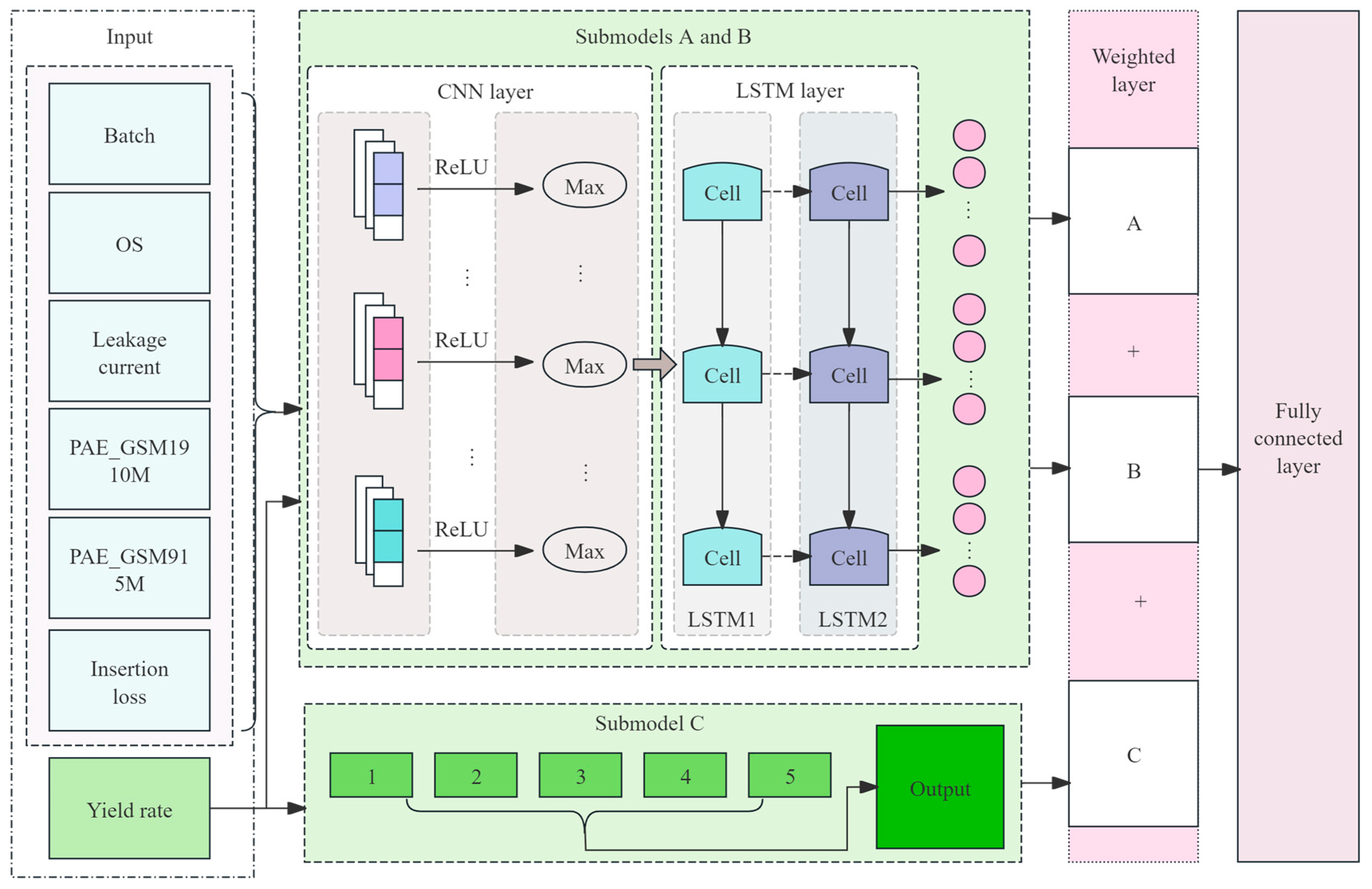
In the methods section of this paper, we have constructed an integrated architecture with multistrategy dynamic weighted fusion aimed at achieving precise prediction of RFFE chip final test yield. A multistrategy fusion model was constructed, extracting the impact of test data on yield from diverse perspectives. Additionally, a dynamic incremental prediction approach was employed, enabling the model to continuously learn and adapt to changes introduced by updated data. The overall architecture is illustrated in Figure 1.
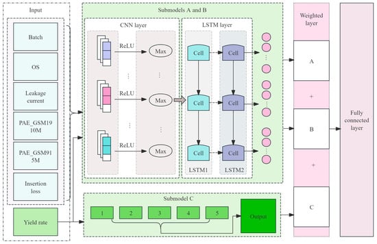
Figure 1.
Overall architecture of yield prediction model.
The architecture is primarily divided into three modules:
- (1)
- Data Preprocessing Module
First, testing metrics are screened and grouped through RF correlation analysis (such as Spearman’s correlation coefficient and VIF evaluation). Principal Component Analysis (PCA) is then employed to reduce the dimensionality of high-dimensional data, extracting key features with high contribution from the original dataset to form an optimized dataset.
- (2)
- Submodel Construction and Fusion Prediction ModuleBased on the preprocessed data, three complementary submodels are developed:
- Submodel A utilizes a CNN-LSTM structure, where convolutional layers extract local features from historical yield data and LSTM captures long-term dependencies, reflecting both short-term fluctuations and long-term trends in process parameters;
- Submodel B employs multichannel inputs to integrate multidimensional electrical and RF test data with historical yield data, thereby revealing the intrinsic relationships among various testing metrics;
- Submodel C adopts an adaptive sliding window averaging strategy that dynamically weights and smooths short-term noise, providing a robust baseline prediction.
Finally, a learnable dynamic weighted fusion mechanism integrates the predictions from all submodels, and a cross-constraint loss is incorporated to ensure consistency in feature representation across submodels, thereby enhancing overall prediction accuracy and robustness.
- (3)
- Dynamic Incremental Training and Prediction Mechanism
To accommodate the continuously changing process conditions during production, a dynamic prediction mechanism is introduced. By quantifying prediction uncertainty through techniques such as Monte Carlo dropout, the system can trigger localized retraining or adjust fusion weights in real time. Additionally, by employing adaptive learning rates and time-decay sample weighting strategies, incremental training is implemented, enabling the model to update continuously, respond rapidly to data fluctuations, and maintain stability and efficiency in real-time predictions.
Overall, this architecture seamlessly integrates dimensionality reduction, temporal feature extraction, multidimensional data fusion, and dynamic adjustment strategies, forming a robust, flexible, and highly accurate yield prediction system for RFFE final testing.
2.1. Establishment of the Dataset
The key test indicators in the mass production test of RFFE chip have a corresponding relationship with the integrated devices. In fact, RFFE chip test is essentially the test of various internal devices, and the setting of its mass production test projects often follows similar principles and logic. The following Table 1 analyzes the different test indexes corresponding to different RF devices.

Table 1.
RFFE test item analysis table.
Open-circuit and short-circuit tests can ensure the connectivity integrity of the internal circuits within the chip. Leakage current testing can verify the chip’s power consumption characteristics. These test items can be categorized as electrical performance metrics. Metrics such as the 1 dB compression point, gain, and vector error further assess the device’s linearity, amplification capability, and signal transmission quality. Additionally, parameters like harmonics, adjacent channel leakage suppression ratio, and switching time effectively control signal purity, spectrum utilization efficiency, and channel switching stability. Noise figure, PAE, insertion loss, and isolation comprehensively ensure overall system performance in terms of noise characteristics, energy efficiency, signal transmission efficiency, and path separation.
The complete signal test items for the RFFE chip encompass all frequency points and internal paths specified in the design. To optimize testing efficiency and reduce testing time, these test items can be organized into groups, with items sharing identical test conditions classified together.
In these test items, PAE refers to Power Added Efficiency. It serves as a critical metric for assessing the performance of radio frequency power amplifiers, indicating the efficiency of converting DC power input into RF output power. Specifically, PAE is determined using the following Formula (1):
where and represent the output and input power, respectively, and is the power consumption supplied by the DC power source, all of which are measured in dBm. This formulation ensures a precise evaluation of the amplifier’s energy conversion efficiency, making PAE a fundamental parameter in RF engineering.
Additionally, ACLR and EVM are influenced by the linearity of the PA (power amplifier), which, in turn, is affected by the power level and gain. Therefore, input and output power, gain, PAE, and power consumption can be grouped for testing. These test parameters reflect the linearity of the power amplifier (PA), which, in turn, influences key metrics such as ACLR and EVM [36].
Therefore, by analyzing the relationships among these test items, it can be concluded that within a test group defined by a specific frequency point (e.g., 824 MHz, 915 MHz, 1910 MHz) or modulation scheme (e.g., QPSK, 64QAM, 256QAM), the PAE test item either influences or is influenced by other test metrics within the same group. Due to the interactions between PAE and other test items, we designate PAE as the characteristic test item among the test items, using it to represent the features of the other test metrics. In addition, there are also electrical test indicators that do not require an RF signal, including the OS group, leakage current group, and insertion loss test group. Therefore, one of the three electrical test groups is also selected as the characteristic test item to ensure that the selected feature data can fully reflect the yield factors. The PAE (PAE_GSM915M, PAE_GSM824M, PAE_QPSK915M, PAE_GSM1910M, PAE_GSM1910M, and PAE_GSM1910M) and the remaining three electrical test indicators (OS group, leakage current group, and insertion loss) were selected as the characteristic test items.
2.1.1. Correlation Analysis of Feature Testing Items
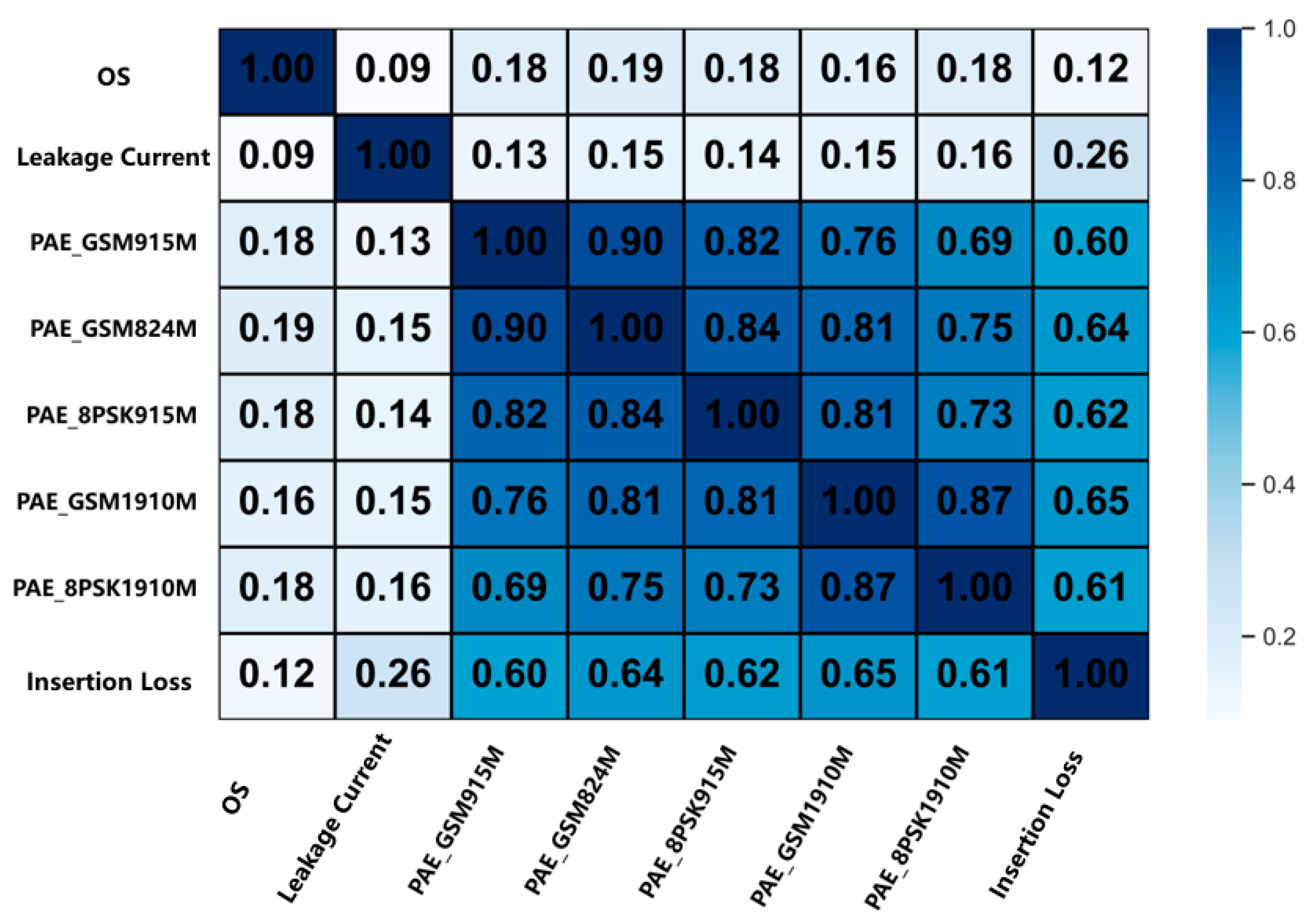
Following data extraction and analysis, we can quantify the interaction between the feature test terms, as shown in Figure 2, to assess their combined effect on yield. Pearson correlation coefficient analysis reveals the correlation between the selected input dataset and the construction of the deep learning model [37].
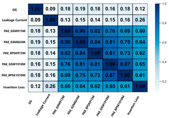
Figure 2.
Thermal map of the correlation coefficient.
The calculated expression is described in Equation (2):
where X and Y both represent different test item data. The value of the correlation coefficient is calculated, where 1 indicates a complete positive correlation, while 0 indicates no linear correlation.
As can be seen in Figure 2, there is a strong correlation between the RF performance test items, with exceeding 0.5. The occurrence of this situation is a normal phenomenon, which also exactly reflects the internal structure characteristics of the RFFE chip. Because the transmission of different frequency point signals is completed by PA, LNA, and other devices inside the chip, the manufacturing defects will affect the transmission and receiving of all frequency point signals. Therefore, the test results of the same test items at different frequency points will generally tend to change in the same trend (high or low), and their correlation is naturally strong. Therefore, PAE_SM915M, PAE_GSM824M, PAE_8 PSK915M, PAE_GSM1910M, and PAE_GSM1910M are not suitable for all the features of the data because of their strong correlation, and subsequent analysis is needed.
All data processing and visualization tasks in this study, including the generation of Figure 2 and subsequent data plotting, were conducted using Python 3.9 within the PyCharm Community Edition 2022.3.3 integrated development environment. Key libraries such as NumPy (1.26.4), Pandas (2.2.2), scikit-learn (1.5.1), and Matplotlib (3.9.0) were utilized for numerical computation, data analysis, machine learning implementation, and plotting, respectively.
Variance inflation factor (VIF) is commonly used to assess the degree of correlation between variables [38]. When VIF values exceed the threshold of 5, it indicates potential multicollinearity. The calculation formula is given in Equation (3):
where = 1, 2,...., j − 1, j refers to the number of influencing factors, is the multiple correlation coefficient, which describes the strength of the correlation, and , the coefficient of determination in the regression model, represents the value obtained from an auxiliary regression where the nth independent variable is regressed on all other independent variables. In this auxiliary regression, the nth independent variable serves as the dependent variable, while the remaining independent variables serve as the independent variables. The value of Rn2 ranges from 0 to 1. The VIF calculation of the above involved test items was performed to analyze their internal correlation degree, and the results are shown in Table 2.
Table 2.
Statistics of collinearity.
From this perspective, the VIF values of four test items have exceeded the conventional limits, and there is multicollinearity among variables. It is not appropriate to use these factors directly for model construction and yield prediction. Therefore, it is necessary to use PCA algorithm to compress the data dimension, deal with the above multicollinearity problems, and screen the data, so as to determine the data suitable for yield evaluation.
2.1.2. Establishing the Dataset Based on PCA
Next, PCA algorithm will be used to extract the principal components representing the data information, so as to select the data with a high contribution rate to the selected principal components, and select a reasonable dataset to improve the evaluation performance of the model.
This study relies on the RFFE mass production test plant project, which involved testing a current 5G RFFE chip, collecting test data from more than 24 million chips, and merging them. Among them, the test time of single chip is about 860 ms, the material transfer time is 300–400 ms, and the comprehensive test time of single chip is about 1.2 s. Considering the actual situation of the factory, under the comprehensive requirements of relatively stable yield change and fault response time, the real-time yield was calculated at 10 minutes, that is, every 500 chips in the chip test were grouped, and a total of 48,609 sets of data were collected.
In total, 48,609 sets of data of 8 test items were analyzed by PCA analysis to calculate the cumulative variance contribution, as shown in Figure 3. When the cumulative variance contribution rate exceeds 95%, these elements can be considered to have captured the core information of the original data.
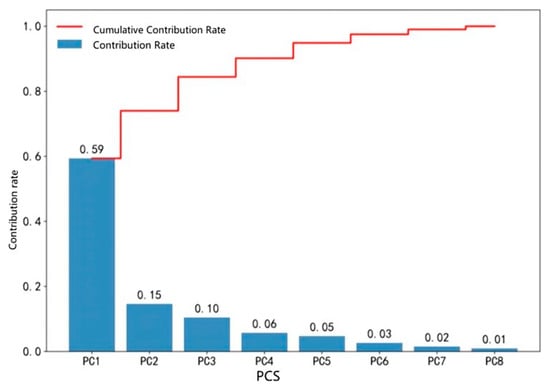
Figure 3.
Contributions rate and cumulative contribution rate of principal components.
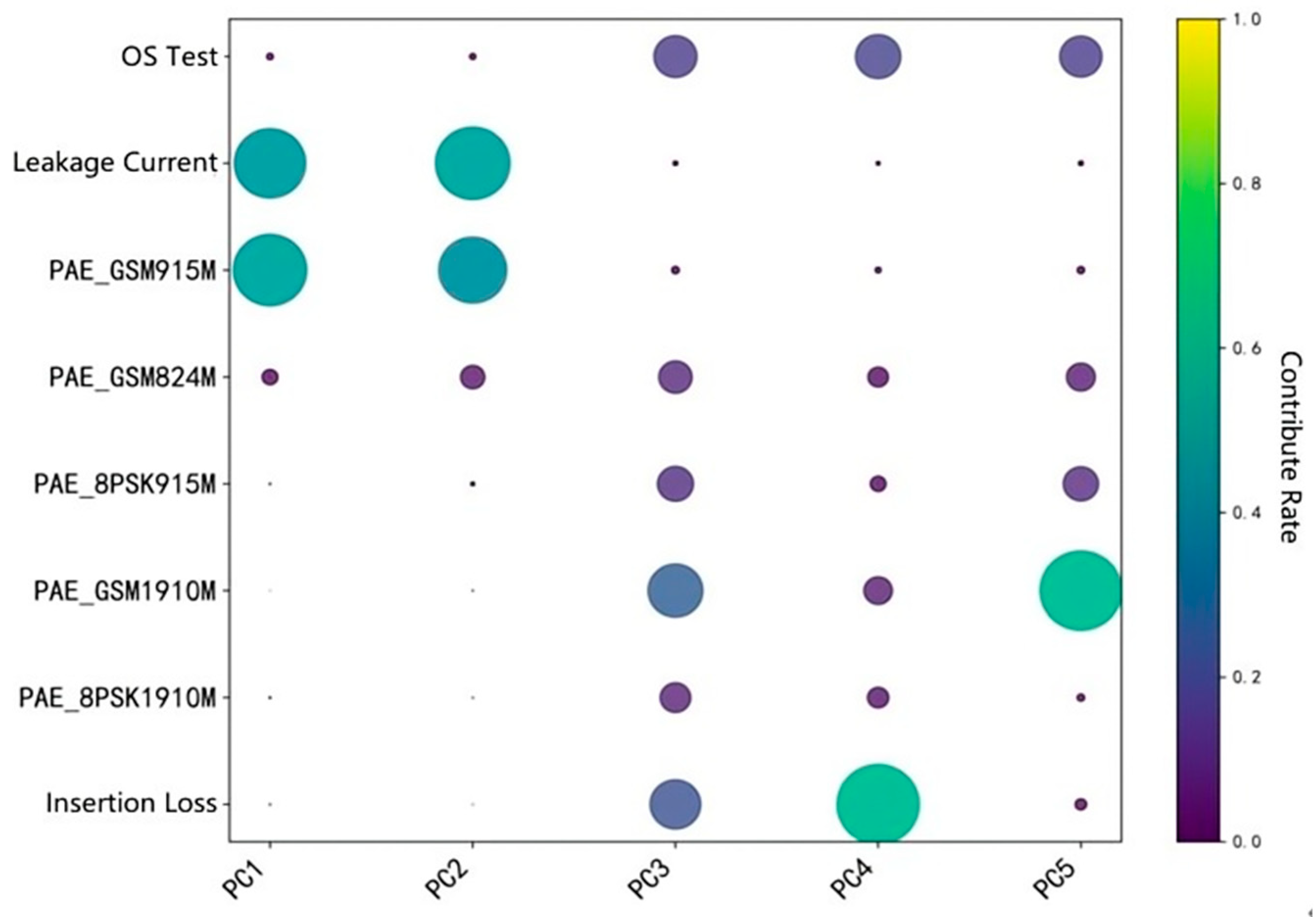
According to the figure, the cumulative contribution rate of the top five factors has reached 95%, so it is decided to select the top five main components. Each principal component is a linear combination of the original features, and different test items will have different weighting coefficients for different principal components. Therefore, the contribution rate of each test item to the top five principal components was counted, as shown in Figure 4.

Figure 4.
Heatmap of the contribution rate of each test item to the top five principal components.
The leakage current, PAE_GSM915M, PAE_GSM1910M, and insertion loss in the test items contribute greatly to each autonomous component, indicating the strong ability of these test items to explain this principal component. The specific calculation results of the contribution rate to the top five principal components and the cumulative contribution rate are shown in Table 3.
Table 3.
Statistical table of the top five principal components.
Although the PAE_GSM824M, PAE_8 PSK915M, and PAE_8 PSK1910M have some impact on the final yield, the contribution of the five principal components is not high, all more than 30%, indicating that their effect on the yield is relatively small or local.
In conclusion, the five test items were selected as characteristic inputs of the model, including the OS test, leakage current, PAE_GSM915M, PAE_GSM1910M, and insertion loss. In addition, batches are also the key indicator affecting the yield. There are certain differences between different batches of chips in the same type, so it is also necessary to classify different batches of chips and be calibrated with different numbers between 0 and 1. Finally, a dataset of batches, five test item failures, and the final yield was formed, as shown in Table 4 below.
Table 4.
RFFE mass production test dataset.
2.2. Establishment of Yield Prediction Submodel
During the final measurement and mass production stages of chips, yield variations are influenced by multiple factors, and the test data exhibit multidimensional inputs and temporal characteristics. Therefore, deep learning models are employed to train and analyze large volumes of test data, aiming to uncover inherent patterns and achieve accurate predictions of chip yield. In this study, a submodel combining CNN-LSTM with sliding window average prediction validation was designed and constructed. By integrating multiple input strategies, this model fully exploits temporal and multidimensional feature information within the data, thereby enhancing prediction performance.
- (1)
- Model A: A CNN-LSTM model for historical yield prediction.
Construct a historical yield prediction Model A based on CNN-LSTM. In the mass production testing of RFFE RF chips, historical yield data often exhibit significant nonlinear fluctuations and local anomalies, which are closely related to short-term variations in different batches of chips and manufacturing process parameters. Model A first utilizes the CNN module, employing input layers, convolutional layers, and pooling layers to extract local features from historical yield data, effectively capturing short-term yield changes caused by sudden shifts in process parameters (such as OS anomalies or PAE deviations). The extracted features are then fed into the LSTM layer, which leverages its input gate, forget gate, and output gate to establish a temporal memory mechanism, modeling global trends arising from factors like process drift, temperature fluctuations, and equipment instability over long periods. This approach compensates for the limitations of single models in deeply mining long-term sequential information. During the final measurement and mass production stages of chips, yield variations are influenced by multiple factors, and the test data exhibit multidimensional inputs and temporal characteristics. Therefore, deep learning models are employed to train and analyze large volumes of test data, aiming to uncover inherent patterns and achieve accurate predictions of chip yield. In this study, a submodel combining CNN-LSTM with sliding window average prediction validation was designed and constructed. By integrating multiple input strategies, this model fully exploits temporal and multidimensional feature information within the data, thereby enhancing prediction performance.
The CNN model ultimately outputs to the input layer of the LSTM to capture timing-dependent data. Its primary purpose is to first use convolutional layers to capture local short-term yield fluctuations and then employ LSTM to model long-term dependencies. This approach not only uncovers the intrinsic characteristics of the yield time series but also largely avoids the issue of information loss caused by long sequences, while ensuring the correlation between yield segments.
- (2)
- Model B: A CNN-LSTM model for historical yield prediction.
Construct a multifeature input yield prediction Model B based on CNN-LSTM. As analyzed during the dataset creation, in addition to the final yield of RFFE chips, the impact of certain test items must also be considered. For example, issues in the PA (power amplifier) process during chip manufacturing can lead to failures in a series of test items, such as output power, gain, and PAE (Power Added Efficiency). Therefore, yield prediction should also account for such feature-related influencing factors. In this context, a multifeature input yield prediction Model B based on CNN-LSTM has been constructed.
Model B is designed to utilize multidimensional feature data collected during the production process (including yield and other process parameters) to more comprehensively capture the intrinsic factors influencing yield variations. By concatenating feature-related influencing factors with historical yield as multichannel inputs, Model B enables the model to simultaneously focus on multiple influencing factors, thereby demonstrating significant advantages in capturing the inherent correlations within the data. The construction method of Model B is similar to that of Model A, with the addition of multiple channels at the input layer, and its construction approach references Model A.
- (3)
- Model C: A sliding window averaging model.
Build submodel C to effectively mitigate the impact of short-term fluctuations and noise inherent in RFFE final test yield data; this study introduces an enhanced sliding window average prediction model (submodel C). Unlike conventional moving average techniques that rely solely on historical yield averages, this submodel integrates adaptive calibration to refine baseline predictions, offering a robust complement to the CNN-LSTM-based submodels. By leveraging past yield data over consecutive timesteps, submodel C computes a smoothed estimate of future yield, serving as a stabilizing reference within the multistrategy fusion framework.
The design of submodel C incorporates the following advanced mechanisms: a dynamic sliding window is defined with a configurable size (set to 5 timesteps in this study, based on empirical analysis of production cycle stability) and a flexible step length. This ensures smooth transitions while maximizing data utilization across varying test conditions. The core computation employs a moving average formula, expressed as:
where represents the moving average at time , is the window size, and denotes the yield at timestep .
To enhance innovation, an adaptive weighting scheme is introduced, adjusting the contribution of each timestep within the window based on its temporal proximity and variance, thereby prioritizing recent and stable data points. This is calculated as:
where is the weight for timestep and is a decay factor tuned to balance responsiveness and smoothness (set to 0.1 after optimization).
This submodel provides a foundational yield estimate, reducing noise interference and short-term anomalies, while its adaptive nature strengthens the fusion process by offering a calibrated baseline that complements the feature-rich predictions of submodels A and B. Its simplicity ensures computational efficiency, making it ideal for real-time deployment in mass production environments.
2.3. Building a Fusion Model
In order to fully utilize the advantages of different submodels, a multistrategy model fusion method was designed. Specifically, by introducing learnable weight layers for the outputs of each submodel, the contribution of each submodel in the final prediction can be dynamically adjusted. The fused output is combined through addition operation and finally generates a comprehensive prediction result through a fully connected layer.
2.3.1. Dynamic Prediction and Incremental Training Mechanism
To adapt to the constantly changing process conditions and environmental factors during the production testing of RFFE chips, we have introduced a multilevel dynamic prediction and incremental training mechanism in the model design. This not only ensures that the model can capture the latest data dynamics in real time but also continuously enhances prediction performance and generalization capabilities through multidimensional adjustment strategies.
- (1)
- Dynamic prediction mechanism with uncertainty quantification
In order to capture real-time data dynamics and adapt the model accordingly, we first quantify the uncertainty of each prediction. We employ a Monte Carlo dropout method, where each input sample x is processed through the model M times with dropout activated.
For each forward pass, a predicted yield is obtained, leading to a set of predictions . The predictive mean and uncertainty (variance) are then computed as follows:
If the uncertainty exceeds a predefined threshold, the system automatically triggers a localized retraining process or readjusts the fusion weights to account for low-confidence predictions.
- (2)
- Adaptive learning rate adjustment
To ensure that the model swiftly adapts to new data during incremental training while maintaining stability, an adaptive learning rate schedule is used. One effective approach is to apply an exponential decay to the learning rate:
where is the initial learning rate, t denotes the current training iteration, and is the decay rate controlling how rapidly the learning rate decreases.
Alternatively, we incorporate adaptive optimization algorithms such as Adam, which update model parameters using the following rule:
where and as estimates of the first and second moments and is a small constant to avoid division by zero.
This adaptive strategy ensures that the model remains responsive to rapid changes in the data while preventing instability due to overly aggressive updates.
- (3)
- Time-decay sample weighting strategy
To better capture the most recent trends in the data during incremental training, we assign weights to training samples based on their recency. Specifically, the weight for sample collected at time (with the current time denoted by ) is given by:
where is a decay constant that determines how quickly the influence of older samples diminishes.
This time-decay weighting strategy ensures that the most recent samples contribute more significantly to the model update, thus enhancing the model’s ability to track the latest yield trends and process parameter changes.
2.3.2. Multistrategy Model Weighted Fusion
Our model leverages multiple submodels to predict yield, including:
- (1)
- Model A: A CNN-LSTM model for historical yield prediction.
- (2)
- Model B: A CNN-LSTM model incorporating multifeatured inputs (electrical and RF parameters).
- (3)
- Model C: A sliding window averaging model.
Each submodel produces a prediction denoted by , , and respectively. These outputs are fused through learnable weights , , and :
In addition to output level fusion, we enforce consistency among the feature representations , , and extracted by each submodel. This is achieved by adding a cross-constraint term to the overall loss function:
where is the primary prediction loss, is a regularization parameter controlling the strength of the cross-constraint, and the sum computes the pairwise Euclidean distance between feature vectors from different submodels, encouraging them to maintain a consistent representation of the input data.
The overall training process integrates the mechanisms described above into a unified framework. The dynamic prediction mechanism continuously evaluates prediction uncertainty, triggering local retraining if needed. The adaptive learning rate adjustment and time-decay sample weighting strategies ensure that the incremental training phase effectively incorporates the most recent data. Simultaneously, multistrategy fusion with cross-constraints aligns feature representations across submodels, leading to a more robust final prediction.
The advantage lies in synthesizing the diverse perspectives of each submodel on the data. Through weighted combination, the model can flexibly adapt to different prediction scenarios.
This integrated approach ensures that the model continuously learns from new data while maintaining consistency across multiple submodels. The combination of these innovations results in a robust, adaptive, and high-precision yield prediction system tailored for the dynamic environment of RFFE chip production testing.
3. Results
Upon completing the construction of the integrated model, the selection of training functions and the configuration of network structure parameters significantly influence model training, thereby affecting the final yield prediction outcomes. Consequently, experiments were conducted to optimize these parameters, fine-tuning the model for precise predictions.
3.1. Selection of Activation Function
The activation function endows the neural network with nonlinear capabilities, enabling effective extraction and interpretation of complex data features. Commonly used activation functions include Sigmoid, Tanh, and ReLU. In this study, simulation experiments were performed to evaluate these options. The fusion model was trained using Sigmoid, Tanh, and ReLU as activation functions, with a 9:1 data split. The model performance is evaluated based on the Mean Absolute Error (MAE) and the Coefficient of Determination (R2).
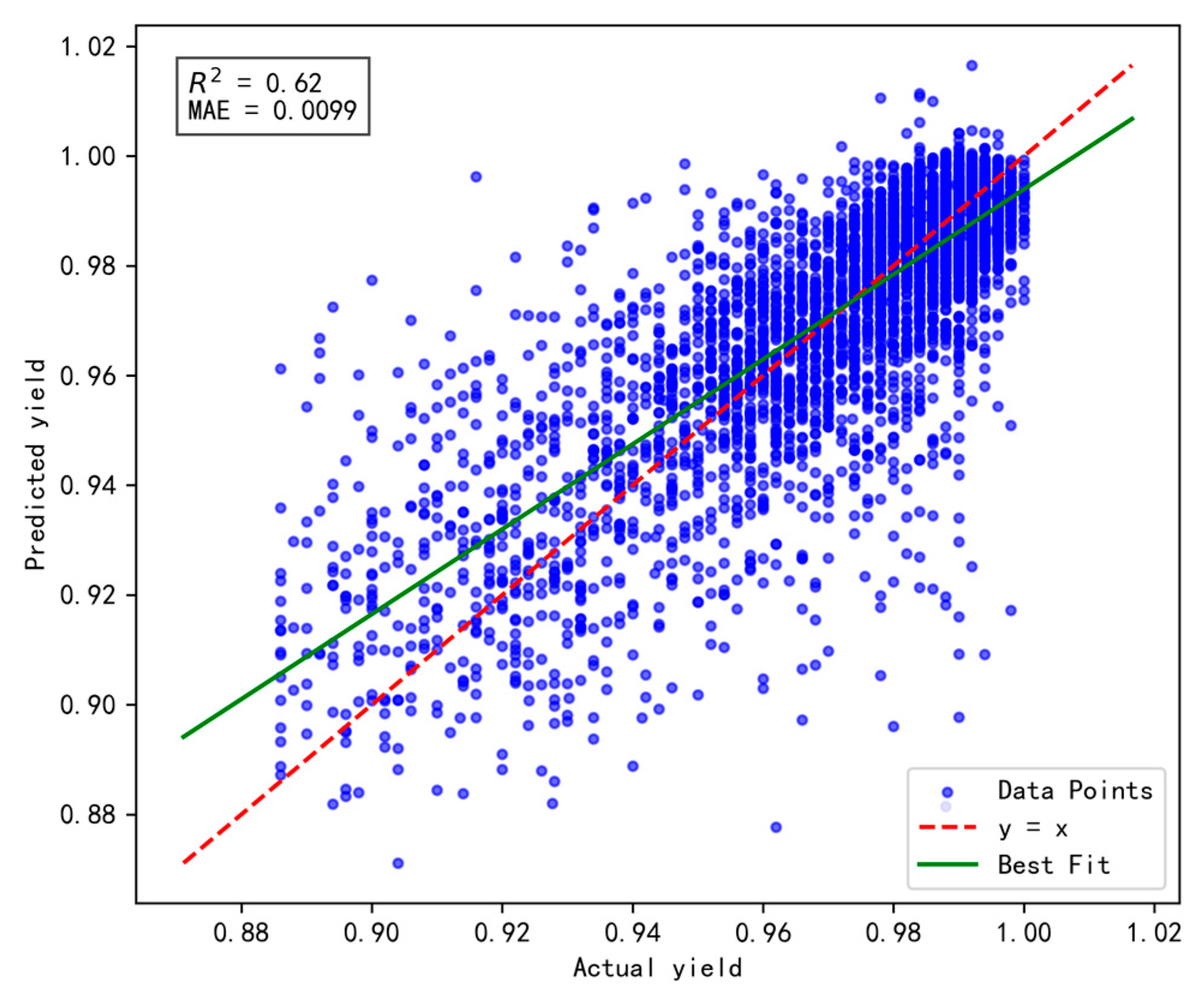
The experimental results are presented in Figure 5, Figure 6 and Figure 7, respectively. Comparative analysis reveals that the Tanh activation function achieves an R2 value of 0.62, representing improvements of 0.02 and 0.08 over the Sigmoid and ReLU functions, respectively. Additionally, its MAE reaches 0.0099, reflecting enhancements of 0.02% and 0.06% compared to Sigmoid and ReLU, respectively. These improvements can be attributed to the advantages of the Tanh activation function, particularly its output range and zero-centered properties.
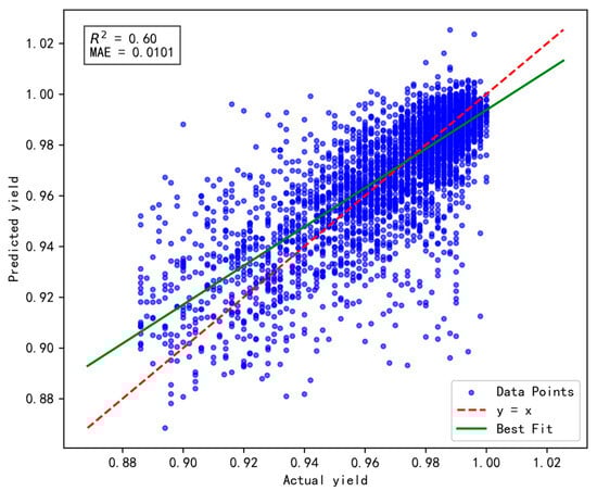
Figure 5.
The impact of Sigmoid activation function on model performance.
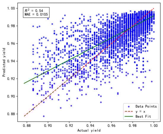
Figure 6.
The impact of ReLU activation function on model performance.

Figure 7.
The impact of Tanh activation function on model performance.
In summary, the Tanh activation function enhances the model’s ability to leverage and interpret factors influencing yield, making it the preferred choice for the hybrid model’s activation function.
3.2. Optimization of Network Structure Parameters
In constructing the CNN-LSTM model, the selection of network parameters impacts prediction outcomes. Following the determination of the activation function, multiple simulation experiments were designed to optimize parameters, including CNN kernel size, pooling method, batch size, LSTM units, iteration count, and Dropout strategy, aiming to establish a CNN-LSTM model for accurate yield prediction. A grid search algorithm was employed to select model parameters and quantify their effects on yield.
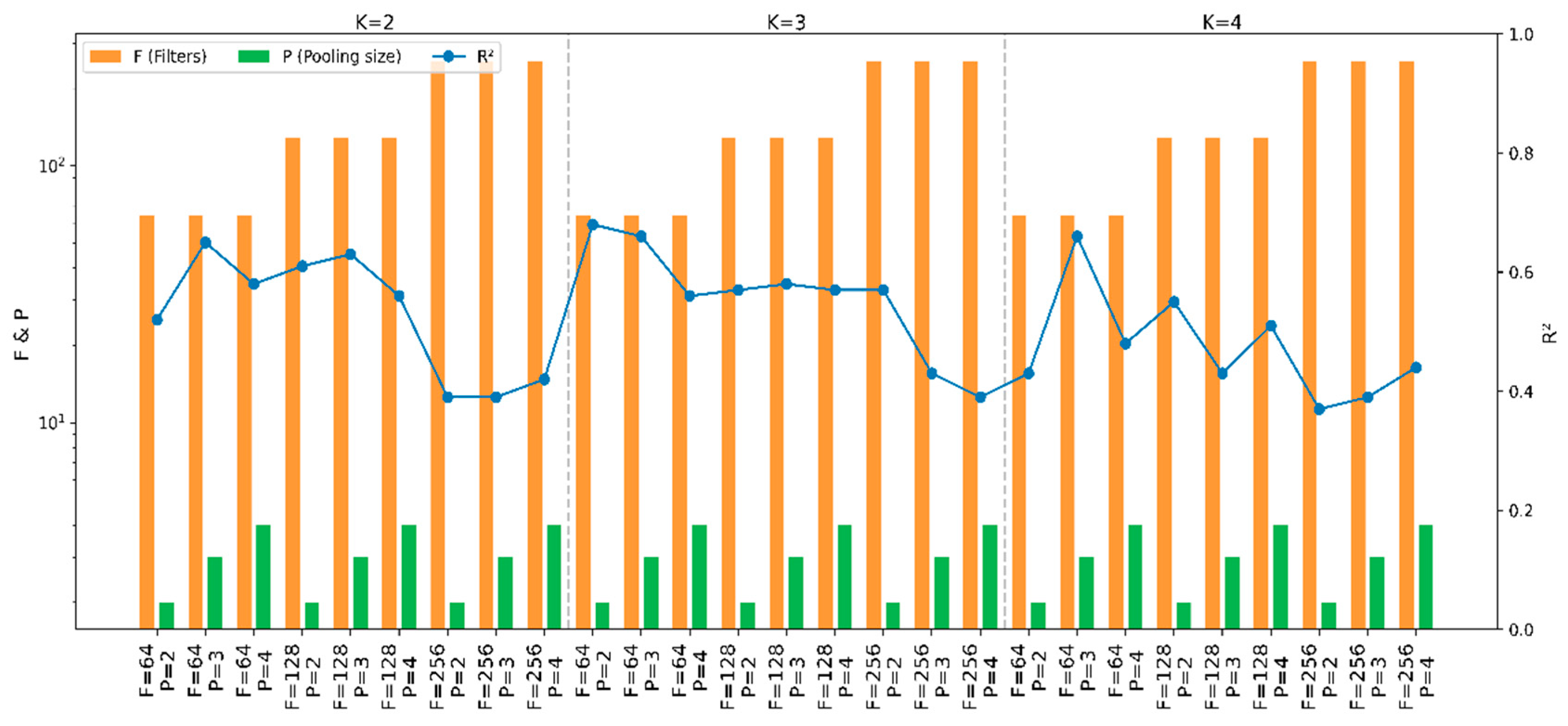
Tuning of CNN internal parameters yielded results shown in Figure 8. Kernel sizes of 2, 3, and 4 were tested, revealing that a kernel size of 3 maximized the coefficient of determination at 0.68. Similarly, filter counts of 64, 128, and 256, and pooling sizes of 2, 3, and 4 were evaluated, with 64 filters and a pooling size of 2 demonstrating superior performance.
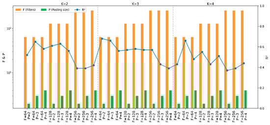
Figure 8.
CNN parameter selection performance chart.
Additionally, optimization was conducted for LSTM units, batch size, epochs, and Dropout. Figure 9 visually illustrates the hyperparameter determination process for the hybrid model.
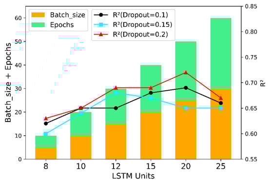
Figure 9.
LSTM parameter selection performance chart.
In the training of this model, the “dropout” technique is utilized, involving the random deactivation of a subset of neurons to facilitate localized updates within the neural network. During the simulation process, the dropout parameters are configured as 0.1, 0.15, and 0.2, respectively, with the specific results presented in Table 5 below.
Table 5.
LSTM parameters and experimental results of model training strategy.
The results indicate that the coefficient of determination (R²) between the evaluated yield and the true values reaches 0.72. This suggests that discarding a portion of the hidden layer neurons with a probability of 20% during training helps reduce dependency on certain local features. Although a dropout parameter of 0.15 yields a higher correlation between the evaluated and true values, a dropout rate of 0.2 is ultimately selected to enhance the model’s generalization ability and mitigate overfitting effects. Based on the above analysis, the grid parameters of the constructed CNN-LSTM fusion model are presented in Table 6.
Table 6.
Hyperparameter selection performance chart.
By configuring the batch size for updates as 5, 10, 15, 20, 25, and 30, it was observed that a batch size of 25 yields a correlation coefficient of 0.72. Additionally, the number of training epochs was set to range from 5 to 30, sampled at intervals of 5, revealing that an epoch counts of 25 also results in a coefficient of determination (R2) of 0.72. When tuning the units of the LSTM neural network, values were tested between 5 and 20 with six increments, and it was found that an LSTM layer size of 20 achieves the highest R² value. For the activation function of the LSTM layer, Tanh was selected, while a dropout rate of 0.2 was adopted as a strategy to prevent overfitting.
3.3. Selection of the Number of Incremental Prediction Samples
To validate the effectiveness and rationality of the proposed dynamic incremental prediction model, the following comparative experiments were designed, with a focus on investigating the impact of the number of incremental prediction samples on model performance. In the experiments, the number of incremental prediction samples was set to 15, 20, 25, and 30, respectively, while R2 (coefficient of determination) and MAE (Mean Absolute Error) were retained as evaluation metrics to comprehensively assess the model’s prediction accuracy and stability. The results are illustrated in Figure 10, Figure 11, Figure 12 and Figure 13 below.

Figure 10.
Results of prediction performance for 15 incremental samples.
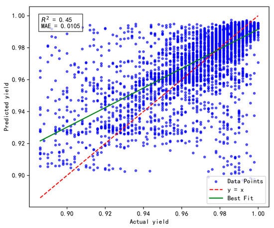
Figure 11.
Results of prediction performance for 20 incremental samples.
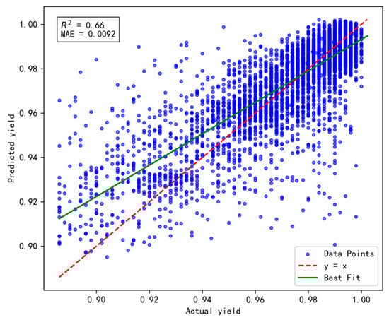
Figure 12.
Results of prediction performance for 25 incremental samples.

Figure 13.
Results of prediction performance for 30 incremental samples.
Based on a comprehensive evaluation using the R2 and MAE metrics, the model achieves optimal performance when the number of incremental prediction samples is set to 25 (R2 = 0.66, MAE = 0.0092), striking an effective balance between data fitting and prediction accuracy. Although the MAE is slightly higher when the number of incremental samples is 15, its R² is lower, indicating insufficient fitting capability. Conversely, when the number of incremental samples reaches 30, both R2 and MAE fail to surpass the performance observed at 25, possibly due to an excessive sample size that prevents the model from promptly adapting to short-term data variations. Therefore, for dynamic incremental prediction, setting the number of samples to 25 is determined to be the optimal choice.
3.4. Model Prediction Yield Assessment and Result Comparison
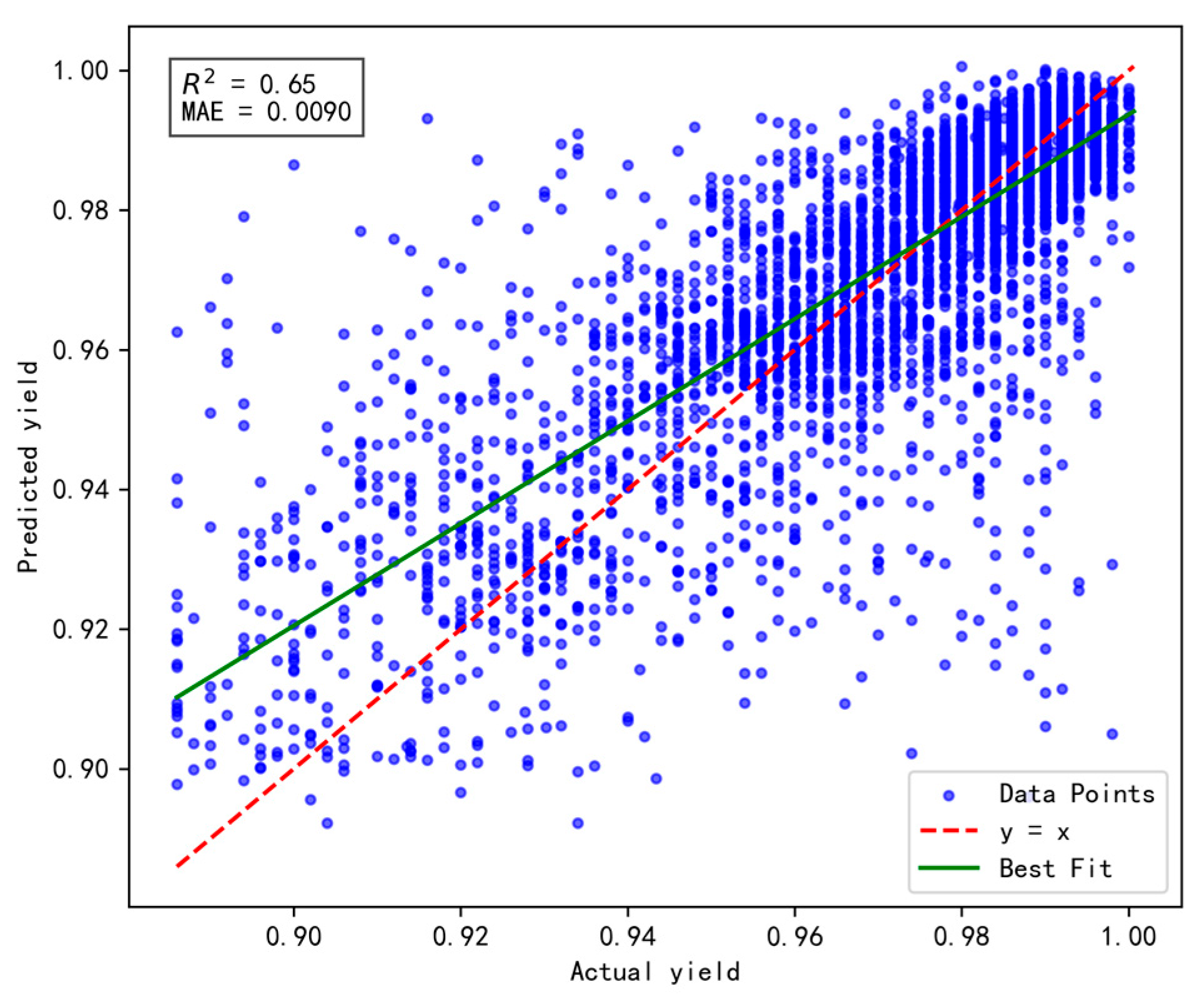
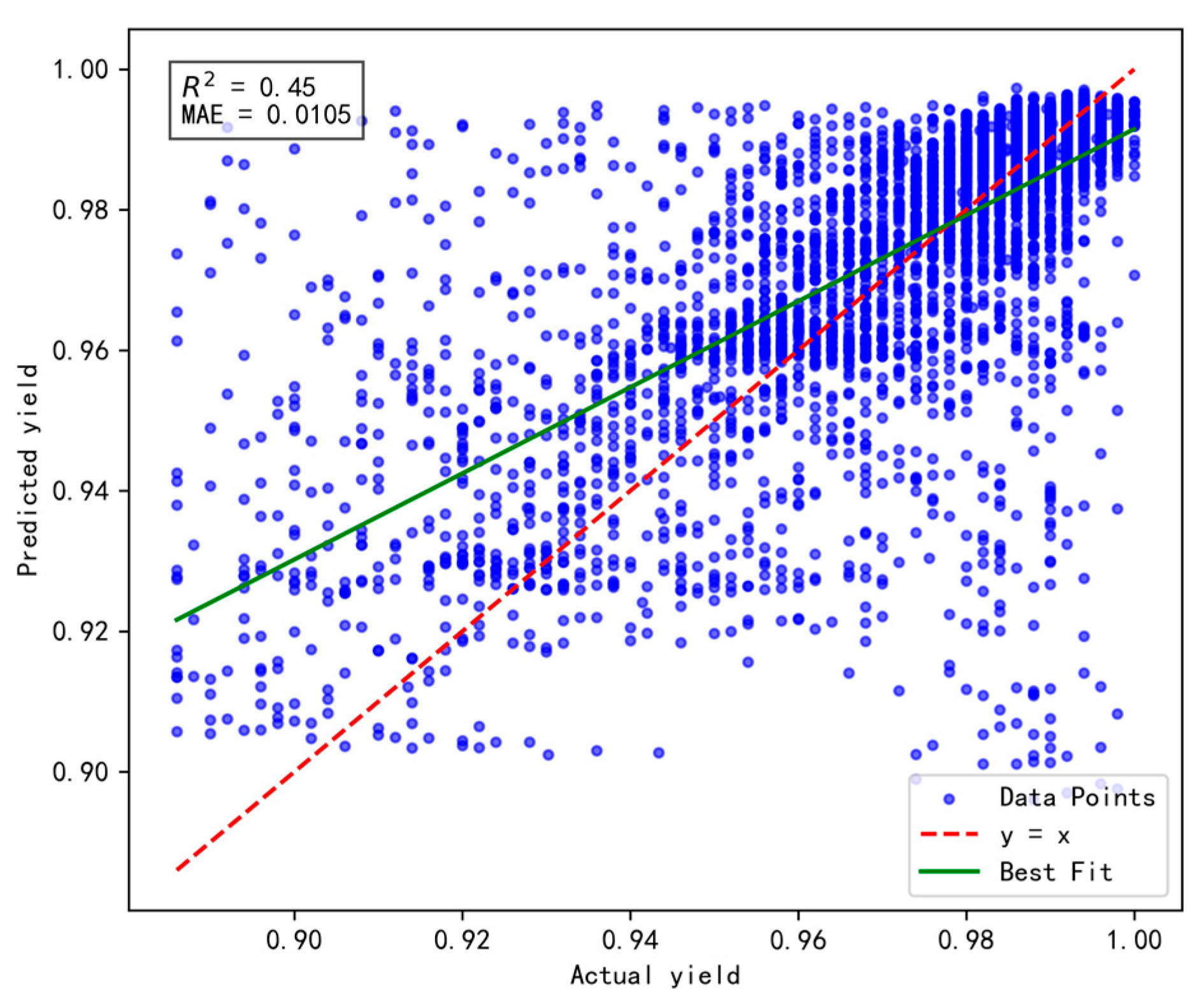
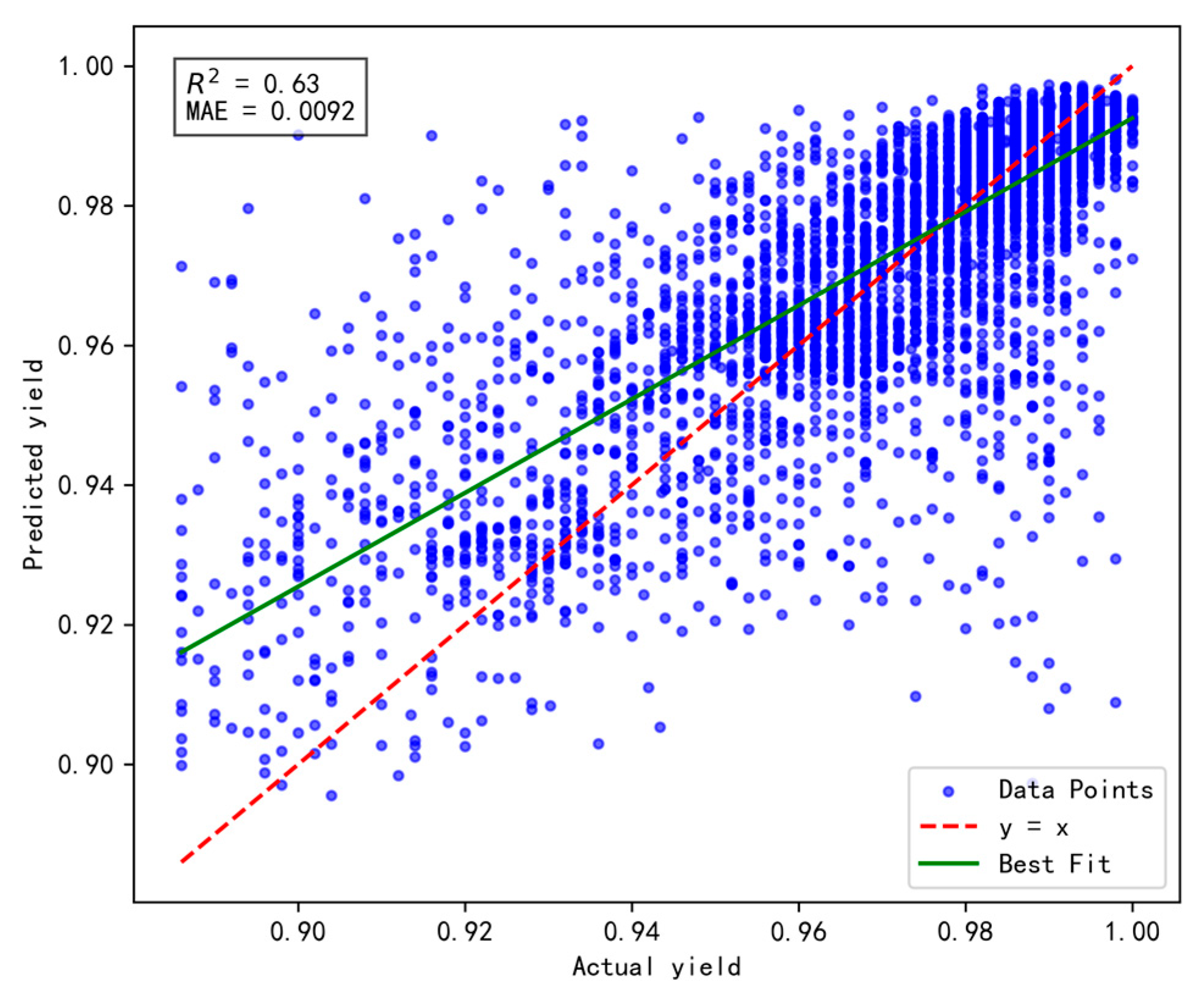
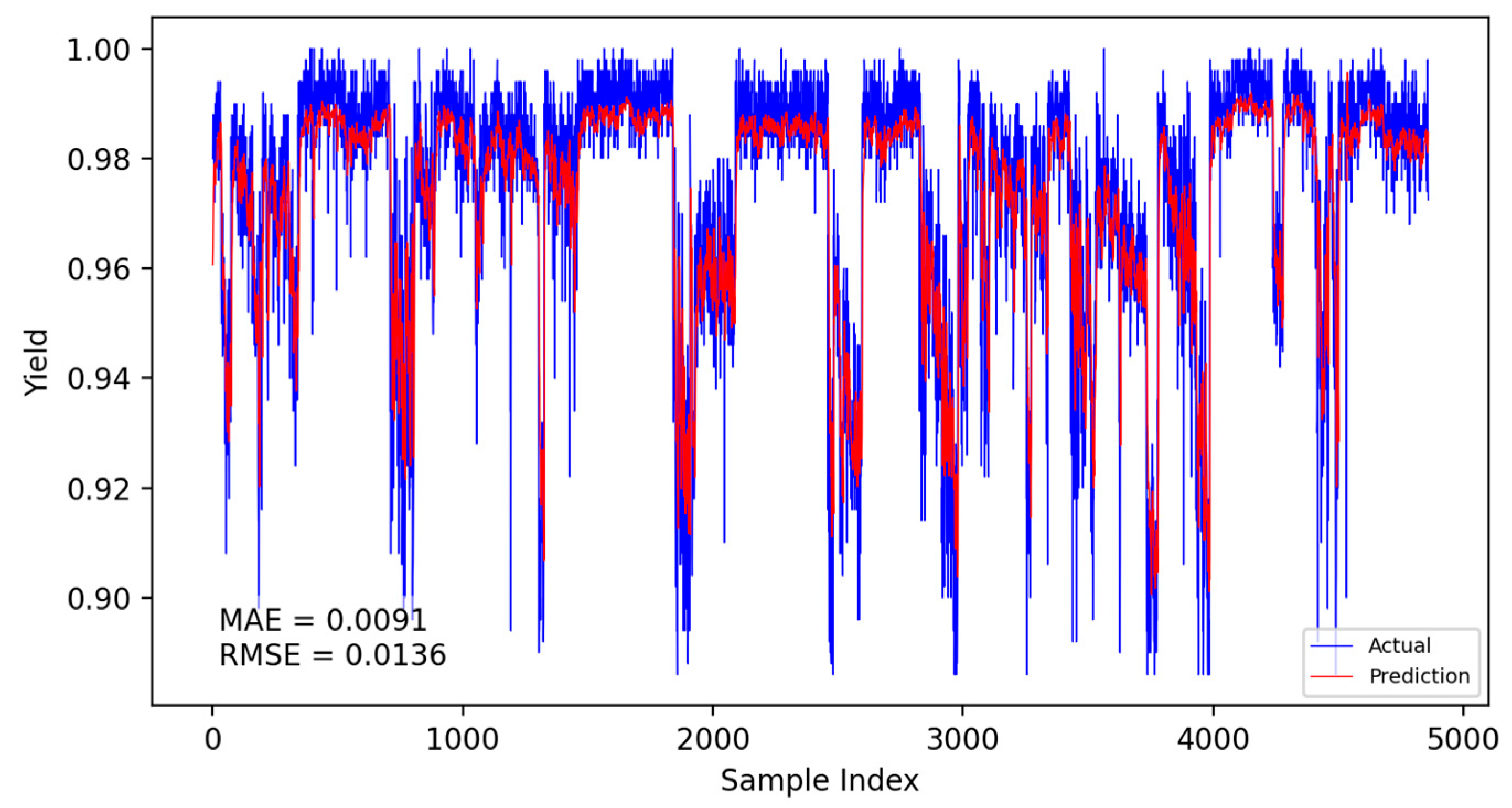
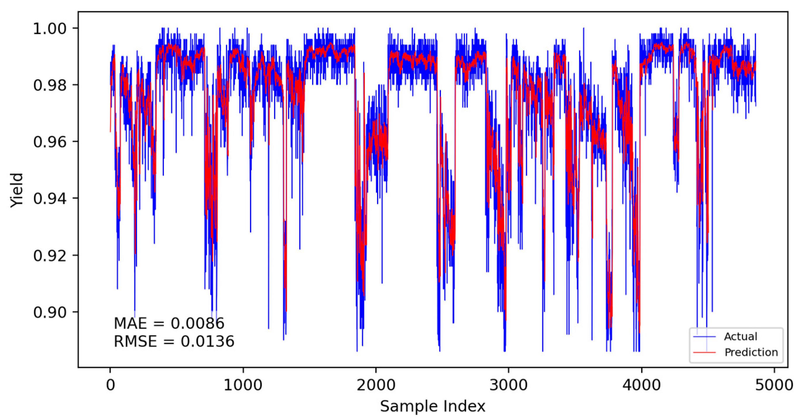
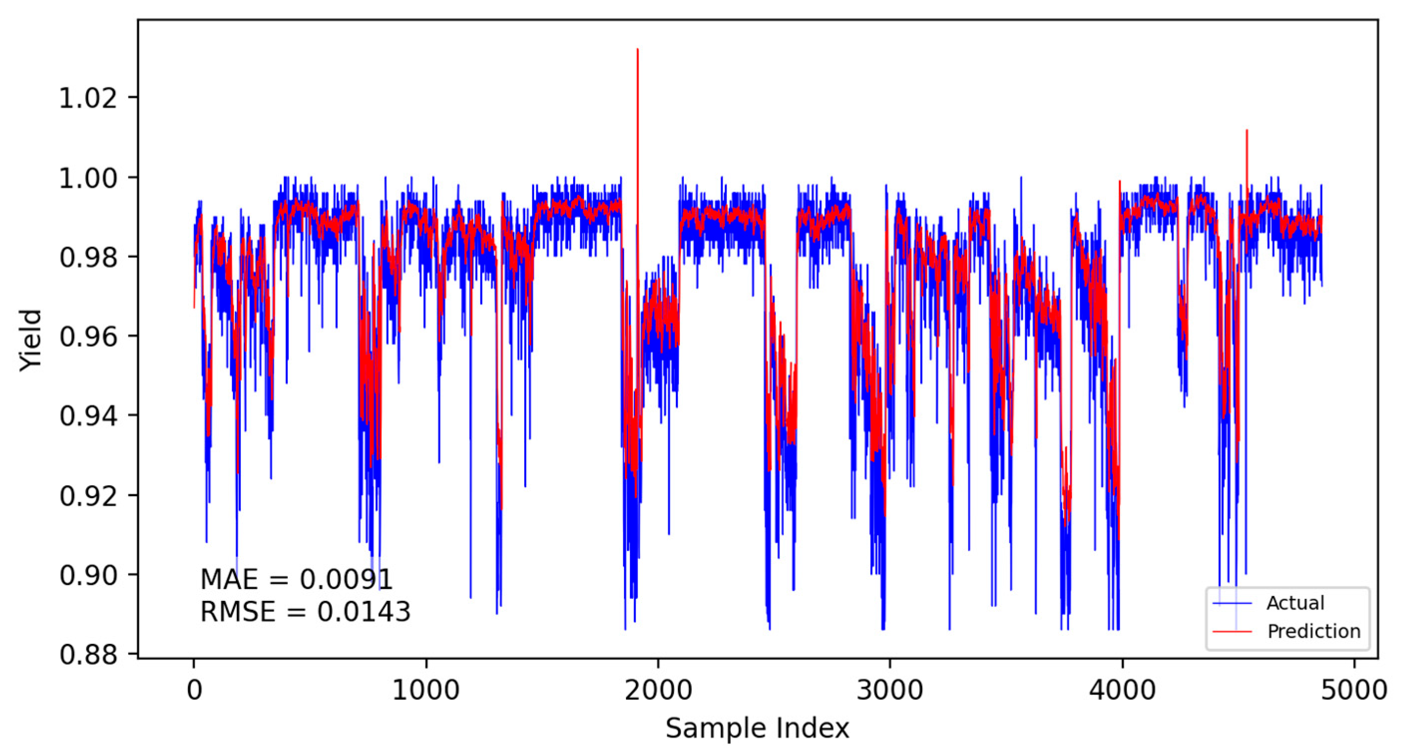
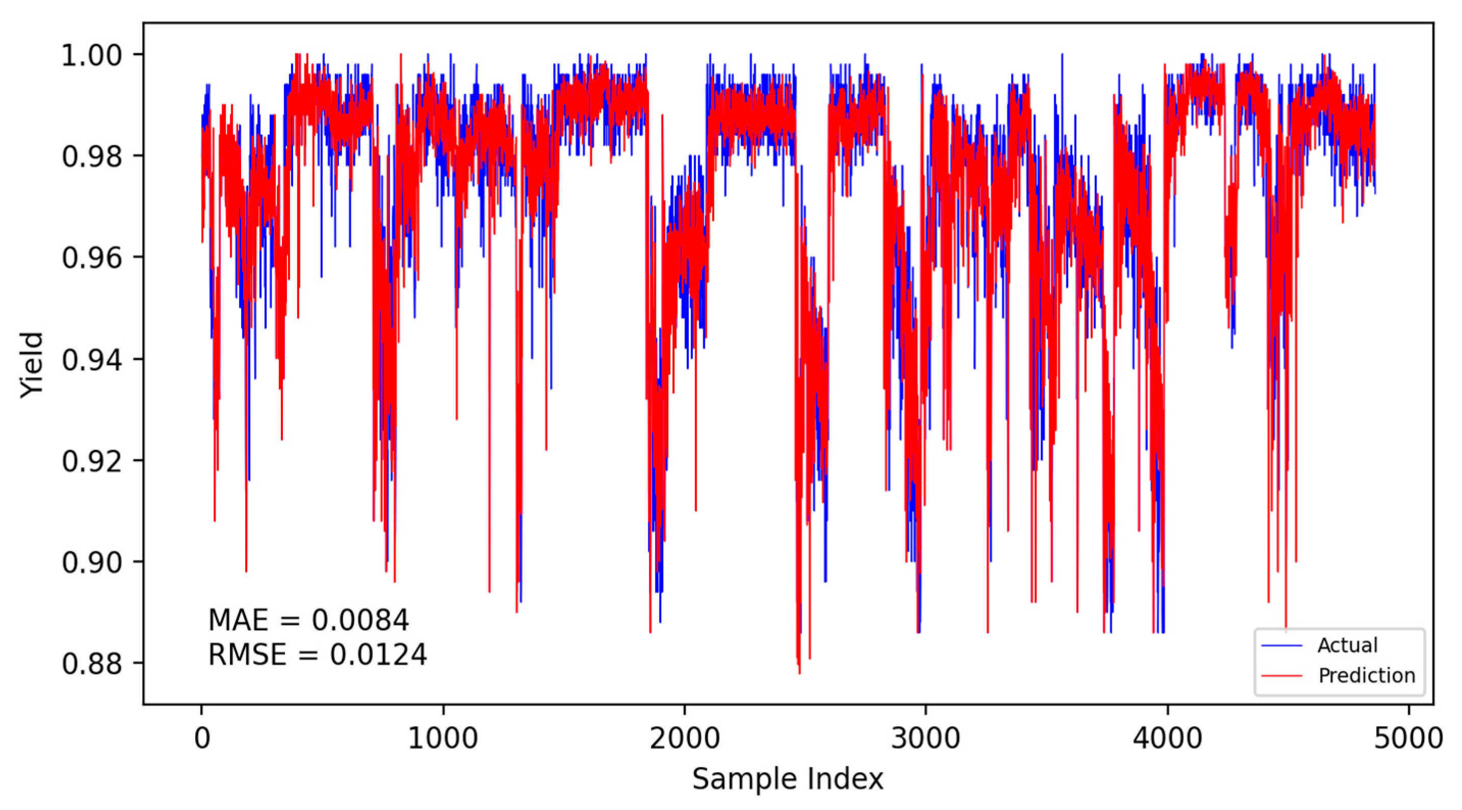
Based on the CNN-LSTM fusion dynamic yield prediction model constructed earlier, along with the optimized parameters and training strategies determined, this section evaluates and compares yield prediction performance. Experiments were conducted using the same dataset and identical training–validation splits. The prediction accuracy of different models was assessed using the Mean Absolute Error (MAE) and Root Mean Square Error (RMSE). Experiments included static and dynamic incremental training predictions for submodel A, submodel B, and the fusion model, with results presented in Figure 14, Figure 15, Figure 16, Figure 17, Figure 18 and Figure 19.
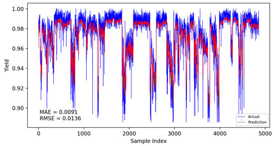
Figure 14.
Submodel A static prediction results.
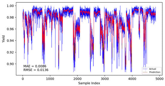
Figure 15.
Submodel A dynamic prediction results.
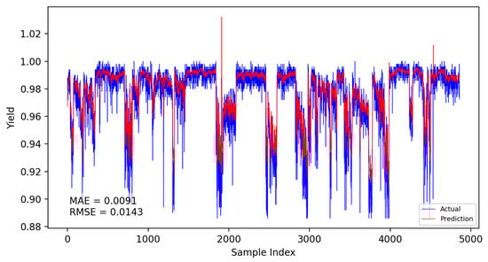
Figure 16.
Submodel B static prediction results.
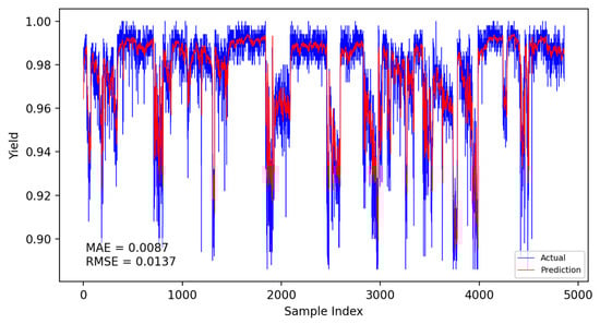
Figure 17.
Submodel B dynamic prediction results.
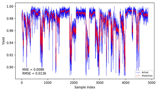
Figure 18.
Fusion model static prediction results.
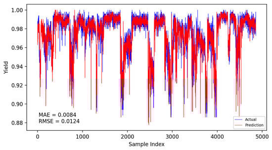
Figure 19.
Fusion model dynamic model prediction results.
The specific comparison of prediction results is shown in the table below, where three models are compared and analyzed using MAE and RMSE performance indicators. The average prediction error of the integrated dynamic model can be as low as 0.0084, which indicates that the yield prediction results can fluctuate within a range of 0.84%. From Table 7, it is evident that the dynamic incremental prediction performance of each model generally surpasses static prediction, with the fusion dynamic prediction model outperforming others. Specifically, its MAE is reduced by 7.69%, 2.33%, 7.69%, 3.45%, and 2.33% compared to other models, while RMSE decreases by 8.82%, 8.82%, 13.29%, 9.49%, and 8.82%, respectively. The dynamic prediction results consistently outperform the static prediction results, indicating that dynamic models, by capturing the time-varying characteristics of the data, can effectively enhance prediction accuracy. The dynamic fusion prediction model achieves the best results, which also suggests that by integrating the advantages of multiple dynamic branches, it can further reduce prediction errors and improve overall performance. Comparative analysis of these results demonstrates that the proposed CNN-LSTM-based multistrategy dynamic weighted fusion yield prediction model exhibits superior reliability and accuracy in yield prediction. The three submodels offer diverse prediction perspectives, optimized through weighting and enhanced by dynamic prediction and incremental training mechanisms, endowing the model with robust adaptability.
Table 7.
Comparison of prediction accuracy among different models.
4. Conclusions
In semiconductor manufacturing, the final testing phase of RFFE chips is pivotal for ensuring product quality and optimizing production efficiency. This study addresses the critical need for accurate yield prediction at this stage, where traditional methods and prior research, predominantly focused on wafer-level analysis, fall short in tackling the unique challenges of final testing—such as test condition variability and complex failure patterns. To this end, we proposed a novel multistrategy dynamic weighted fusion model integrating Convolutional Neural Networks (CNNs), Long Short-Term Memory (LSTM) networks, and sliding window averaging, tailored specifically for RFFE mass production testing.
The methodology leverages a three-pronged approach. First, a rigorous RF correlation parameter selection process, employing Spearman’s correlation coefficient and variance inflation factors (VIF), identified key test metrics—such as multifrequency PAE, OS test, leakage current, and insertion loss—mitigating multicollinearity via Principal Component Analysis (PCA) to construct an optimized dataset from over 24 million RFFE chip test records. Second, three submodels were developed: submodel A (CNN-LSTM) captures historical yield trends, submodel B integrates multidimensional features for intrinsic yield insights, and submodel C employs adaptive sliding window averaging to provide stable baselines, collectively enhancing prediction diversity. Third, a dynamic weighted fusion mechanism, augmented by incremental training with Monte Carlo uncertainty quantification and adaptive learning rates, integrates these submodels, ensuring adaptability to production dynamics.
Experimental evaluation demonstrated the model’s superior performance. With optimized parameters—including Tanh activation, a batch size of 25, 20 LSTM units, and a dropout rate of 0.2—the fusion model achieved a Mean Absolute Error (MAE) of 0.84% and a Root Mean Square Error (RMSE) of 1.24% on a consistent dataset. Compared to static and single submodel predictions, the dynamic fusion model reduced MAE by up to 7.69% and RMSE by up to 13.29%, underscoring its enhanced accuracy and reliability. The Tanh activation function’s zero-centered properties and the multiperspective submodel design proved instrumental in capturing complex data patterns, while incremental training endowed the model with robust adaptability to real-time production shifts.
This study’s contributions are threefold: it introduces an efficient test parameter grouping strategy based on RF device correlations, develops a versatile submodel framework leveraging temporal and feature diversity, and establishes a dynamic fusion model with incremental training for precise yield forecasting. These advancements not only fill a research gap in RFFE final test yield prediction but also offer practical benefits, such as reduced testing time, improved process optimization, and enhanced cost-efficiency, aligning with the stringent timelines of modern chip manufacturing.
Despite these achievements, limitations remain. The computational complexity of incremental training may pose challenges for real-time deployment in resource-constrained environments. Future work could explore lightweight optimization techniques, such as model pruning or quantization, to enhance efficiency without sacrificing accuracy. Additionally, extending the model to incorporate multistage production data or adapting it to other semiconductor devices could further broaden its applicability. Overall, this research lays a solid foundation for advancing yield prediction in RFFE manufacturing, contributing to the technological evolution and economic viability of the RF chip industry.
Author Contributions
Conceptualization, Y.L., Y.C., and X.Y.; methodology, Y.L., Y.C., and X.Y.; software Y.C., writing—review and editing Y.L., Y.C., and X.Y. All authors have read and agreed to the published version of the manuscript.
Funding
This work was funded by the Major Science and Technology Projects of Zhongshan City (2024A1018), the Key Research and Development Plan Project of Heilongjiang (JD2023SJ19), the Natural Science Foundation of Heilongjiang Province (LH2023F034), and the Science and Technology Project of Heilongjiang Provincial Department of Transportation (HJK2024B002).
Data Availability Statement
The data supporting the findings of this study are not publicly available due to commercial confidentiality restrictions. These data were obtained from a proprietary chip production testing project and are subject to privacy and ethical constraints imposed by the data provider.
Conflicts of Interest
The authors declare no conflicts of interest.
References
- Dai, R.; Ren, J.; He, J.; Xiao, J.; Kong, W. RFFE Integration Design for 5G in 0.13 um RFSOI Technology. In Proceedings of the 2019 China Semiconductor Technology International Conference (CSTIC), Shanghai, China, 18–19 March 2019; pp. 1–3. [Google Scholar]
- Madakam, S.; Lake, V.; Lake, V.; Lake, V. Internet of Things (IoT): A literature review. J. Comput. Commun. 2015, 3, 164. [Google Scholar]
- Wu, B.; Qi, Q.; Liu, L.; Liu, Y.; Wang, J. Wearable aerogels for personal thermal management and smart devices. ACS Nano 2024, 18, 9798–9822. [Google Scholar] [CrossRef] [PubMed]
- Racha, G.; Kishore, K.L.; Kamatham, Y.; Perumalla, S.R. Design Methodology of Radio Frequency Front End Power Amplifier Topologies for Sub-6 GHz Applications. In Proceedings of the 2024 2nd International Conference on Recent Trends in Microelectronics, Automation, Computing and Communications Systems (ICMACC), Hyderabad, India, 19–21 December 2024; pp. 598–603. [Google Scholar]
- Dixit, E.; Rani, S. Integrated Trends, Opportunities, and Challenges of 5G and Internet of Things. In Current and Future Cellular Systems: Technologies, Applications, and Challenges; John Wiley & Sons: New York, NY, USA, 2025; pp. 139–152. [Google Scholar]
- Sahu, A.; Aaen, P.H.; Devabhaktuni, V.K. Advanced technologies for next-generation RF front-end modules. Int. J. RF Microw. Comput.-Aided Eng. 2019, 29, 21700. [Google Scholar]
- van Klompenburg, T.; Kassahun, A.; Catal, C. Crop yield prediction using machine learning: A systematic literature review. Comput. Electron. Agric. 2020, 177, 105709. [Google Scholar] [CrossRef]
- Goel, S.K.; Marinissen, E.J. On-chip test infrastructure design for optimal multi-site testing of system chips. In Proceedings of the Design, Automation and Test IEEE Conference in Europe, Munich, Germany, 7–11 March 2005; pp. 44–49. [Google Scholar]
- Moyne, J.; Iskandar, J. Big data analytics for smart manufacturing: Case studies in semiconductor manufacturing. Processes 2017, 5, 39. [Google Scholar] [CrossRef]
- Sun, D.; Hu, Y. Address the Challenges of Mass Production Testing for 5G Millimeter Devices. In Proceedings of the 2024 Conference of Science and Technology for Integrated Circuits (CSTIC), Shanghai, China, 17–18 March 2024; pp. 1–5. [Google Scholar]
- Yan, K.; Sun, D. Ultra-Wideband (UWB) Test Solution On V93000. In Proceedings of the 2023 China Semiconductor Technology International Conference (CSTIC), Shanghai, China, 26–27 June 2023; pp. 1–5. [Google Scholar]
- Baykas, T.; Sum, C.S.; Lan, Z.; Wang, J.; Rahman, M.A.; Harada, H.; Kato, S. IEEE 802.15.3c: The first IEEE wireless standard for data rates over 1 Gb/s. IEEE Commun. Mag. 2011, 49, 114–121. [Google Scholar] [CrossRef]
- Gomes, R.; Hammoudeh, A.; Caldeirinha, R.F.; Al-Daher, Z.; Fernandes, T.; Reis, J. Towards 5G: Performance evaluation of 60 GHz UWB OFDM communications under both channel and RF impairments. Phys. Commun. 2017, 25, 527–538. [Google Scholar] [CrossRef]
- Pancera, E.; Timmermann, J.; Zwick, T.; Wiesbeck, W. Quantification of the Effect of the Non-Idealities in UWB Systems. In Proceedings of the Fourth European Conference on Antennas and Propagation, Barcelona, Spain, 12–16 April 2010; pp. 1–4. [Google Scholar]
- Shome, P.P.; Khan, T.; Koul, S.K.; Antar, Y.M. Filtenna designs for radio-frequency front-end systems: A structural-oriented review. IEEE Antennas Propag. Mag. 2020, 63, 72–84. [Google Scholar]
- Hentschel, T.; Fettweis, G.; Tuttlebee, W. The digital front-end: Bridge between RF and baseband processing. In Software Defined Radio: Enabling Technologies; Wiley: Hoboken, NJ, USA, 2002; pp. 151–198. [Google Scholar]
- Kattenborn, T.; Leitloff, J.; Schiefer, F.; Hinz, S. Review on Convolutional Neural Networks (CNN) in vegetation remote sensing. ISPRS J. Photogramm. Remote Sens. 2021, 173, 24–49. [Google Scholar] [CrossRef]
- Yu, Y.; Si, X.; Hu, C.; Zhang, J. A review of recurrent neural networks: LSTM cells and network architectures. Neural Comput. 2019, 31, 1235–1270. [Google Scholar] [CrossRef]
- Mirza, A.I.; O’Donoghue, G.; Drake, A.W.; Graves, S.C. Spatial yield modeling for semiconductor wafers. In Proceedings of the SEMI Advanced Semiconductor Manufacturing Conference and Workshop, Cambridge, MA, USA, 13–15 November 1995; pp. 276–281. [Google Scholar]
- Jang, S.J.; Kim, J.S.; Kim, T.W.; Lee, H.J.; Ko, S. A Wafer Map Yield Prediction Based on Machine Learning for Productivity Enhancement. IEEE Trans. Semicond. Manuf. 2019, 32, 400–407. [Google Scholar]
- Dong, H.; Chen, N.; Wang, K. Wafer yield prediction using derived spatial variables. Qual. Reliab. Eng. Int. 2017, 33, 2327–2342. [Google Scholar] [CrossRef]
- Wang, H.; Li, B.; Tong, S.; Chang, I.; Wang, K. A discrete spatial model for wafer yield prediction. A discrete spatial model for wafer yield prediction. Qual. Eng. 2018, 30, 169–182. [Google Scholar] [CrossRef]
- Dan, J.; Weihua, L.; Nagarajan, R. Semiconductor Manufacturing Final Test Yield Optimization and Wafer Acceptance Test Parameter Inverse Design Using Multi-Objective Optimization Algorithms. IEEE ACCESS 2021, 9, 137655–137666. [Google Scholar]
- Busch, R.; Wahl, M.; Choubey, B. Wafer yield prediction using AI: Potentials and pitfalls. In Proceedings of the Metrology, Inspection, and Process Control XXXVII, San Jose, CA, USA, 27 February–2 March 2023; SPIE: Bellingham, WA, USA, 2023. [Google Scholar]
- Ahmadi, A.; Stratigopoulos, H.-G.; Nahar, A.; Orr, B.; Pas, M.; Makris, Y. Harnessing fabrication process signature for predicting yield across designs. In Proceedings of the 2016 IEEE International Symposium on Circuits and Systems (ISCAS), Montreal, QC, Canada, 22–25 May 2016; pp. 898–901. [Google Scholar]
- Lee, Y.; Roh, Y. An expandable yield prediction framework using explainable artificial intelligence for semiconductor manufacturing. Appl. Sci. 2023, 13, 2660. [Google Scholar] [CrossRef]
- Zhai, W.; Han, Q.; Chen, L.; Shi, X. Explainable automl (xautoml) with adaptive modeling for yield enhancement in semiconductor smart manufacturing. In Proceedings of the 2024 2nd International Conference on Artificial Intelligence and Automation Control (AIAC), Guangzhou, China, 20–22 December 2024; pp. 162–171. [Google Scholar]
- Jiang, D.; Lin, W.; Raghavan, N. A Gaussian mixture model clustering ensemble regressor for semiconductor manufacturing final test yield prediction. IEEE Access 2021, 9, 22253–22263. [Google Scholar] [CrossRef]
- Xu, Q.; Xu, C.; Wang, J. Forecasting the yield of wafer by using improved genetic algorithm, high dimensional alternating feature selection and SVM with uneven distribution and high-dimensional data. Auton. Intell. Syst. 2022, 2, 24. [Google Scholar]
- Zhang, Y.; Zheng, J.; Jiang, Y.; Huang, G.; Chen, R. A text sentiment classification modeling method based on coordinated CNN-LSTM-attention model. Chin. J. Electron. 2019, 28, 120–126. [Google Scholar]
- Shi, M.; Yang, B.; Chen, R.; Ye, D. Logging curve prediction method based on CNN-LSTM-attention. Earth Sci. Inform. 2022, 15, 2119–2131. [Google Scholar] [CrossRef]
- Wan, A.; Chang, Q.; Al-Bukhaiti, K.; He, J. Short-term power load forecasting for combined heat and power using CNN-LSTM enhanced by attention mechanism. Energy 2023, 282, 128274. [Google Scholar] [CrossRef]
- Borré, A.; Seman, L.O.; Camponogara, E.; Stefenon, S.F.; Mariani, V.C.; Coelho, L.d.S. Machine fault detection using a hybrid CNN-LSTM attention-based model. Sensors 2023, 23, 4512. [Google Scholar] [CrossRef] [PubMed]
- Elmaz, F.; Eyckerman, R.; Casteels, W.; Latré, S.; Hellinckx, P. CNN-LSTM architecture for predictive indoor temperature modeling. Build. Environ. 2021, 206, 108327. [Google Scholar] [CrossRef]
- Chung, W.H.; Gu, Y.H.; Yoo, S.J. District heater load forecasting based on machine learning and parallel CNN-LSTM attention. Energy 2022, 246, 123350. [Google Scholar]
- Tomoya, K.; Osamu, M.; Haris, G. Performance Analysis of OFDM with Peak Cancellation Under EVM and ACLR Restrictions. IEEE Trans. Veh. Technol. 2020, 69, 6230–6241. [Google Scholar]
- Rahadian, H.; Bandong, S.; Widyotriatmo, A.; Joelianto, E. Image encoding selection based on Pearson correlation coefficient for time series anomaly detection. Alex. Eng. J. 2023, 82, 304–322. [Google Scholar]
- Gómez, S.R.; García, G.B.C.; Pérez, G.J. A Redefined Variance Inflation Factor: Overcoming the Limitations of the Variance Inflation Factor. Comput. Econ. 2024, 65, 337–363. [Google Scholar]


Disclaimer/Publisher’s Note: The statements, opinions and data contained in all publications are solely those of the individual author(s) and contributor(s) and not of MDPI and/or the editor(s). MDPI and/or the editor(s) disclaim responsibility for any injury to people or property resulting from any ideas, methods, instructions or products referred to in the content. |
© 2025 by the authors. Licensee MDPI, Basel, Switzerland. This article is an open access article distributed under the terms and conditions of the Creative Commons Attribution (CC BY) license (https://creativecommons.org/licenses/by/4.0/).