Lasso-Based k-Means++ Clustering

Abstract

Clustering is a powerful and efficient technique for pattern recognition which improves classification accuracy. In machine learning, it is a useful unsupervised learning approach due to its simplicity and efficiency for clustering applications. The curse of dimensionality poses a significant challenge as the volume of data increases with rapid technological advancement. It makes traditional methods of analysis inefficient. Sparse clustering is essential for efficiently processing and analyzing large-scale, high-dimensional data. They are designed to handle and process sparse data efficiently since most elements are zero or lack information. In data science and engineering applications, they play a vital role in taking advantage of the natural sparsity in data to save computational resources and time. Motivated by recent sparse k-means and k-means++ algorithms, we propose two novel Lasso-based k-means++ (Lasso-KM++) clustering algorithms, Lasso-KM1++ and Lasso-KM2++, which incorporate Lasso regularization to enhance feature selection and clustering accuracy. Both Lasso-KM++ algorithms can shrink the irrelevant features towards zero, and select relevant features effectively by exploring better clustering structures for datasets. We use numerous synthetic and real datasets to compare the proposed Lasso-KM++ with k-means, k-means++ and sparse k-means algorithms based on the six performance measures of accuracy rate, Rand index, normalized mutual information, Jaccard index, Fowlkes–Mallows index, and running time. The results and comparisons show that the proposed Lasso-KM++ clustering algorithms actually improve both the speed and the accuracy. They demonstrate that our proposed Lasso-KM++ algorithms, especially for Lasso-KM2++, outperform existing methods in terms of efficiency and clustering accuracy.

1. Introduction

The primary goal of clustering is to organize data points with similar features into well-defined groups. The foundation and earliest applications of clustering were presented in Driver and Kroeber [1], where they used clustering techniques to classify cultural traits across different societies, identifying patterns and relationships among cultural elements. As an early form of clustering, Zubin [2] developed a method of quantifying “like-mindedness” among individuals for analyzing psychological data. A density-based clustering algorithm, DBSCAN, was introduced by Ester et al. [3], which identifies clusters of arbitrary shapes and handles noise without requiring a predefined number of clusters. Wang [4] considered a novel clustering technique that leverages morphological operations to connect adjacent data points and form distinct connected domains. Sharma [5] proposed an s-divergence-based internal clustering validation index for evaluating the compactness and separation of clusters, improving the reliability of internal validation metrics. Lukauskas and Ruzgas [6] extended the clustering method based on the modified, inversion formula density estimation to overcome previous limitations, particularly in high-dimensional cases.

Clustering is an unsupervised machine learning technique that groups similar data points into clusters, where objects within a cluster are more similar to each other and they differ between clusters. Clustering algorithms are very useful tools in data science [7]. Unsupervised learning algorithms, such as k-means clustering, are widely used to partition datasets into distinct groups based on inherent similarities. The field of unsupervised learning has become increasingly interested in clustering in recent decades. In clustering algorithms, they can be mainly divided into two approaches. One is a probability-model-based approach [8], and the other is a nonparametric approach [9]. In the probability-model-based approach, the expectation maximization (EM) algorithm is widely used for probabilistic clustering in Gaussian mixture models [10,11,12]. In general, there are many popular nonparametric clustering algorithms in the literature. These are mean-shift [13,14,15], spectral clustering [16,17,18], k-means [19,20,21], fuzzy c-means [22,23,24], and possibilistic c-means [25,26,27], and so forth. In this paper, we focus on the k-means algorithm of the nonparametric approach.

The k-means algorithm was proposed by MacQueen [28] in 1967. The algorithm partitions the datasets into k clusters with the idea that objects within the same cluster are similar to each other, while objects between clusters are dissimilar. In k-means clustering, the average squared distance between points within the same cluster is minimized. It is a popular method for clustering data in unsupervised learning. The k-means clustering has various extensions and has been applied in a variety of substantive areas in the literature [29,30,31,32,33]. However, the k-means clustering algorithm is usually affected by initialization. To address this challenge, the k-means++ (KM++) algorithm [34] has presented a specified procedure for initializing cluster centers before proceeding with k-means optimization. The random selection of initial centroids in k-means may result in inadequate suboptimal clustering results. This problem is addressed by KM++ which generates initial centroids that are separated from one another, improving convergence and also clustering performance. There have been more studies on KM++, such as Xu et al. [35], Pin et al. [36] and Vardakas and Likas [37]. These clustering algorithms may be effective for low-dimensional data, but they may not work well for high-dimensional datasets. In general, data with high-dimensional features may include unimportant characteristics or sparsity. That is, some feature components become insignificant and so feature selection/reduction techniques need to be considered for clustering high-dimensional datasets.

Clustering effectiveness may suffer due to the existence of redundant or irrelevant features in high-dimensional data. All features are handled equally in classical clustering techniques, which may result in poor cluster formation and more computing complexity. In this case, feature selection within the clustering process may ensure that only the most informative features contribute to cluster formation. It is the process of identifying and retaining the most relevant features in a dataset by eliminating irrelevant, redundant, or noisy ones. In general, the feature selection technique is commonly used in clustering and machine learning to improve model performance, reduce computational complexity, and enhance interpretability as the following descriptions:

• Minimizing the Dimensionality Curse: Clustering becomes more challenging in high-dimensional data space because the distances between points make it harder to define clusters effectively. Many clustering algorithms, including k-means, rely on distance metrics, such as Euclidean distance, which can become unreliable when many irrelevant features dilute the true structure of datasets. Feature selection helps by retaining only the most informative dimensions, making cluster structures more distinguishable.
• Eliminating Irrelevant and Noisy Features: High-dimensional datasets often contain irrelevant or noisy features that do not contribute to meaningful clustering, but instead introduce randomness. Selecting only the most informative features reduces noise, leading to more robust and well-defined clusters.
• Improving Clustering Accuracy and Stability: Classical clustering algorithms treat all features equally, even when some are uninformative or redundant. Feature selection with different feature weights ensures that clustering is based on the most discriminative features, leading to more accurate and stable cluster assignments.

In regression, the theory of variable selection is widely recognized. Tibshirani [38] first proposed the idea of least absolute shrinkage and selection operator (Lasso) as a variable selection method in regression models. Lasso can shrink variable coefficients towards zero and ultimately render some of them exactly zero. Afterward, Witten and Tibshirani [39] proposed a novel framework for feature selection in k-means clustering, called sparse k-means (S-KM). In S-KM, Witten and Tibshirani [39] used Lasso for data observations to obtain adaptively a chosen subset of features. Based on the possibilistic c-means (PCM) framework, Yang and Benjamin [40] introduced sparse PCM (SPCM) clustering with Lasso which integrates sparsity constraints into the PCM algorithm. Recently, two sparse k-means (S-KM) methods, S-KM1 and S-KM2, were proposed in [41]. We know that the k-means algorithm is the most well-known and popular method for clustering data, and k-means++ provides a good initialization technique to improve the convergence and clustering performance of k-means. However, both k-means and k-means++ are not good at handling high-dimensional data due to a lack of feature selection and the existence of redundant or irrelevant features in high-dimensional datasets. Thus, in S-KM, S-KM1 and S-KM2 clustering, feature selection was incorporated based on the L₁ penalty as an extension to k-means clustering so that it improves k-means with feature selection technique for reducing redundant or irrelevant features in high-dimensional data. In spite of its effectiveness, S-KM, S-KM1 and S-KM2 may suffer several shortcomings as follows: (1) Poor Cluster Initialization: First, they still rely on k-means initialization, especially in high-dimensional data, which can lead to unstable cluster assignments and convergence to poor local optima. (2) Sensitivity to Noise and Outliers: Since they are based on k-means which relies on squared Euclidean distances, they are highly sensitive to outliers and can be influenced by noisy features. (3) Computational Complexity: In addition, L₁ penalized optimization adds computational overhead compared to k-means. (4) The assumption of Cluster Format: Another limitation of them assumes spherical clusters due to its use of Euclidean distance metric, making it less effective for irregular cluster structures.

On the other hand, SPCM in [40] introduced sparsity into the PCM clustering framework, and thus, it improves PCM with a feature selection technique for reducing redundant or irrelevant features in high-dimensional data. However, the method also has drawbacks as follows: (1) Mode-Seeking Behavior and Sensitivity to Initialization: SPCM suffers from mode-seeking behavior that is similar to PCM, meaning that clusters tend to form around high-density regions (modes) rather than being well-separated. In addition, poor initialization may lead to empty or redundant clusters. (2) Difficulty in Balancing Membership: The SPCM with sparse constraints needs to be carefully tuned to avoid excessive sparsity, which can result in unstable clusters. (3) Parameter Sensitivity: The SPCM algorithm requires a careful selection of parameters, such as the sparsity level and scale parameters, making them harder to use in practice. (4) The Assumption of Cluster Format: Due to its use of Euclidean distance, SPCM needs to assume a spherical cluster structure in datasets, which will make it less effective in real applications.

According to these limitations highlighted above, improving clustering algorithms that effectively combine robust initialization, sparsity constraints, and efficient cluster formation is our goal. Motivated by KM++, S-KM1, and S-KM2, we propose Lasso-KM1++ and Lasso-KM2++ clustering algorithms. The Lasso-KM1++ algorithm, similar to S-KM1, is subject to the Lasso constraint. The other Lasso-KM2++ clustering algorithm, similar to S-KM2, includes a penalty term of feature weights in KM++. To achieve their sparse solution, Lasso-KM1++ and Lasso-KM2++ are capable of discarding these undesirable features towards zero exactly. Numerous synthetic and real datasets are used to evaluate the performance of the proposed Lasso-KM1++ and Lasso-KM2++ algorithms by several experiments and their effectiveness compared with the existing methods, such as k-means, KM++, S-KM1 and S-KM2. The efficiency and usefulness of the proposed Lasso-KM1++ and Lasso-KM2++ algorithms are demonstrated by comparisons and results from experiments. Both current S-KM2 and proposed Lasso-KM2++ integrate penalty terms in their objective functions to promote feature sparsity, ensuring that only the most relevant features contribute to clustering. However, Lasso-KM2++ holds a distinct advantage over S-KM2 due to its superior initialization strategy. While S-KM2 relies on standard k-means initialization, which can be highly sensitive to initial centroid selection, poor cluster assignments in some cases and prone to poor local optima, Lasso-KM2++ applies KM++ initialization, which strategically selects initial centroids in a way that enhances convergence and cluster quality. This makes Lasso-KM2++ more robust, especially in datasets with complex structures or high-dimensional feature spaces. The remaining sections of the paper are organized as follows: In Section 2, we describe the proposed Lasso-KM1++ and Lasso-KM2++ algorithms. Based on synthetic and real datasets, Section 3 presents the comparisons between the proposed S-KM++ and k-means, KM++, S-KM1 and S-KM2 algorithms based on several different performance measures. We further make a comparative analysis for these compared clustering algorithms. Finally, we make conclusions and suggestions for future research in Section 4.

2. The Proposed Lasso-KM1++ and Lasso-KM2 ++ Clustering Algorithms

In this section, we propose the Lasso-KM1++ and Lasso-KM2++ clustering algorithms, motivated by the KM++, S-KM1 and S-KM2. Let $X=\left\{x_1,x_{2,}\dots ,x_n\right\}$ and $A=\left\{a_1,a_2,\dots ,a_c\right\}$ be the dataset and cluster centers in a p-dimensional Euclidean space ${ℝ}^p$. Let the membership matrix be $U={[u_{ik}]}_{n\times c}$, $i=1,2,\dots ,n,k=1,2,\dots ,c$ with $n\times c$ membership values, where $u_{ik}\in \{0,1\},$ $i=1,2,\dots ,n$, $k=1,2,\dots ,c$ are binary variables in which if the data point i belongs to the cluster k, then $u_{ik}$ is one; otherwise, it is zero. The membership of a data point $x_i$ to the cluster k is hard-assigned in the k-means clustering, which means that each point is only associated with one cluster. The membership variable $u_{ik}=1$, if $x_i$ is assigned to the cluster k, otherwise 0. The binary membership matrix $U$ contains all $u_{ik}$ values, where each row sums to 1, meaning each point belongs to only one cluster. The objective function of k-means clustering aims to minimize the sum of squared distances between data points and their assigned cluster centroids, where the membership indicator $u_{ik}$ is a key component of this function.

Thus, the objective function of k-means with $k^{th}$ cluster center $a_k$ and membership $u_{ik}$ is defined by $J_{KM}\left(U,V\right)={\displaystyle \sum _{i=1}^n{\displaystyle \sum _{k=1}^c{u}_{ik}{d}^2\left(x_i,a_k\right)}}$, where the Euclidean distance $d\left(x_i,a_k\right)=‖x_i-a_k‖=\sqrt{{\displaystyle {\sum }_{j=1}^p{(x_{ij}-a_{kj})}^2}}$ is used. The k-means algorithm works by iterating the necessary conditions to minimize the objective function $J_{KM}\left(U,V\right)$ using updated equations for cluster centers and memberships. The updated equations for the cluster centers $a_k$ and membership function $u_{ik}$ are $a_k={\displaystyle \sum _{i=1}^n{u}_{ik}{x}_{ij}}/{\displaystyle \sum _{i=1}^n{u}_{ik}}$ and $u_{ik}=\left\{\begin{array}{l}1;\mathrm{if} {‖x_i-a_k‖}^2=\underset{1\le k\le c}{\min }{‖x_i-a_k‖}^2\\ 0;\mathrm{otherwise}\end{array}\right.,$ $1\le k\le c,1\le i\le n$. The term $‖x_i-a_k‖$ is the Euclidean distance between the data point $x_i$ and the cluster center $a_k$. The k-means is widely used, but it includes some drawbacks, especially related to how cluster centroids are initialized. The k-means algorithm faces issues with random initialization, which can cause poor clustering results and slow convergence. Due to intelligent centroids initialization, the k-means++ algorithm improves initial cluster selection.

In general, k-means++ initially selects cluster centers that are well dispersed in the data space, which often leads to faster convergence and more accurate clustering results. The k-means++ algorithm is more flexible to data variations and is less likely to become trapped in local minima. These initialization steps for the k-means++ algorithm can be briefly described as follows: The first centroid $a_1$ is selected uniformly at random from the dataset X. Then, calculate the Euclidean distance between each data point and the nearest centroid. The next centroid $a_k$ needs to be chosen with a probability proportional to the Euclidean distance to the nearest cluster centroid. In this probabilistic distribution, points located farther away from existing centroids are more likely to be chosen. Compared with k-means, the k-means++ algorithm provides notable improvements and enhancements. We describe the k-means++ algorithm as follows:

In the k-means++ algorithm, an arbitrary set of cluster centers is used as a starting point. Let $D\left(x_i\right)$ denote the shortest distance from a data point $x_i$ to the closest center $a$ that we already selected. Then, the k-means++ considers the following procedures:

(1)

Select the first centroid $a_1$ uniformly at random from the dataset X.

(a)

For each remaining data point $x_i$, compute its squared distance from the nearest chosen centroid with $D\left(x_i\right)=\underset{a\in A}{\min }‖x_i-a‖$ where $a$ is the selected centroids.

(b)

Assign $P\left(x_i\right)$ as the probability of choosing $x_i$ as the next centroid $a_i={x^{\prime }}_i\in X$, with probability $P\left(x_i\right)=D{\left({x^{\prime }}_i\right)}^2/{\displaystyle \sum _{x_i\in X}D{\left(x_i\right)}^2}$. The probability of selecting a point that is farther from the existing centroid is higher.

(2)

In Steps (a)–(b), repeat the process until the total of k centroids is determined.

(3)

Run k-means clustering using these k centroids: (i) assign each data point to its nearest centroid. (ii) update centroids by computing the mean of assigned points. (iii) repeat until centroids converge, or a stopping criterion is met.

On the other hand, Yang and Parveen [41] recently proposed the S-KM1 and S-KM2 methods. The S-KM1 objective function was defined as $\underset{U,V,w}{\max }\left[{\displaystyle \sum _{j=1}^p{w}_j\left\{\frac{1}{n}{\displaystyle \sum _{i=1}^n{\displaystyle \sum _{i^{\prime }=1}^n{(x_{ij}-x_{i^{\prime }j})}^2-\left({\displaystyle \sum _{i=1}^n{\displaystyle \sum _{k=1}^c{u}_{ik}{\left(x_{ij}-a_{kj}\right)}^2}}\right)}}\right\}}\right]$ subject to ${‖w‖}_2^2\le 1,{‖\mathrm{w}‖}_1\le s,w_j\ge 0\forall j$, where $w_j$ is the feature weight for the feature $j$ with condition ${‖w‖}_2^2\le 1$ and the number of dimension is $p$ in datasets. The updated equations are as follows:

$$\begin{array}{cc}{\displaystyle \underset{U,V}{min}}\left[{\displaystyle \sum _{j=1}^p}{w}_j{\displaystyle \sum _{i=1}^n}{\displaystyle \sum _{k=1}^c}{u}_{ik}{\left(x_{ij}-a_{kj}\right)}^2\right]{\mathrm{subject}\mathrm{to}\parallel w\parallel }_2^2\le 1,{\parallel \mathrm{w}\parallel }_1\le s,w_j\ge 0\forall j\hfill & \left(\mathrm{i}\right)\hfill \\ {\displaystyle \underset{w}{max}}\left\{w^{T}a\right\}\hfill & \left(\mathrm{ii}\right)\hfill \\ u_{ik}=\left[\begin{array}{c}1,\mathrm{if}{\displaystyle \sum _{j=1}^p}{w}_j{\left(x_{ij}-a_{kj}\right)}^2={\displaystyle \underset{1\le l\le c}{min}}{\displaystyle \sum _{j=1}^p}{w}_j{\left(x_{ij}-a_{lj}\right)}^2,1\le k\le c,1\le i\le n\hfill \\ 0,\mathrm{otherwise}\hfill \end{array}\right.\hfill & \left(\mathrm{iii}\right)\hfill \\ a_k={\displaystyle \sum _{i=1}^n}{u}_{ik}{x}_{ij}/{\displaystyle \sum _{i=1}^n}{u}_{ik}\hfill & \left(\mathrm{iv}\right)\hfill \end{array}\}$$

(1)

Let us consider $a_j$ to be $a_j={\displaystyle \frac{1}{n}}{\displaystyle {\displaystyle \sum _{i=1}^n}{\left(x_{ij}-{\overline{x}}_j\right)}^2}-\left[{\displaystyle {\displaystyle \sum _{i=1}^n}{\displaystyle \sum _{k=1}^c{u}_{ik}{\left(x_{ij}-v_{kj}\right)}^2}}\right]$, where ${\overline{x}}_j={\displaystyle {\sum }_{i=1}^n{x}_{ij}}/n$. To maximize $\left[{\displaystyle \sum _{j=1}^p{w}_j\left\{\frac{1}{n}{\displaystyle \sum _{i=1}^n{\displaystyle \sum _{i^{\prime }=1}^n{(x_{ij}-x_{i^{\prime }j})}^2-\left({\displaystyle \sum _{i=1}^n{\displaystyle \sum _{k=1}^c{u}_{ik}{\left(x_{ij}-a_{kj}\right)}^2}}\right)}}\right\}}\right]$ w.r.t $w_j\forall j=1,2,\dots ,p$ with fixed $U={[u_{ik}]}_{n\times c}$ and $A=\left\{a_1,a_2,\dots ,a_c\right\}$, is similar to the equation defined by $\underset{w}{\max }\left\{w^{T}a\right\}$ of (ii) in Equation (1) subject to ${‖\mathrm{w}‖}_1\le s,{‖w‖}_2^2\le 1,w_j\ge 0\forall j$, where $a_k$ is the cluster center and $U={\left[u_{ik}\right]}_{n\times c}$ is the membership matrix of size $n\times c$ with binary variable $u_{ik}\in \{0,1\}$. The optimization of the S-KM1 objective function w.r.t. the membership $u_{ik}$ is exactly the same as k-means. Thus, the updated formula (iii) of Equation (1) should be $u_{ik}=1$ if $x_i$ data point belongs to the $k^{th}$ cluster, and otherwise 0. The feature weights vector is $w=\left[w_1,w_2,\dots ,w_p\right]\in R^p$ and $w=S(a,\Delta )/{‖S(a,\Delta )‖}_2,$ where the solution of $\underset{w}{\max }\left\{w^{T}a\right\}$ with $w=S(a,\Delta )/{‖S(a,\Delta )‖}_2$ is given in [41] as the following Proposition 1.

Proposition 1.

[41]. The convexity defined in Equation (1), that is $\underset{w}{\max }\left\{w^{T}a\right\}$ subject to the constraints ${‖\mathrm{w}‖}_1\le s, {‖w‖}_2^2\le 1 \forall j,w_j\ge 0$, can be resolved by using the soft-thresh holding operator $S$ defined as $w={\displaystyle \frac{S(a,\Delta )}{{‖S(a,\Delta )‖}_2}}$, where the soft thresh holding operator $S(a,\Delta )$ is defined by $S(a,\Delta )=\left[S(a_1,\Delta ),\dots ,S(a_d,\Delta )\right]$ with $S\left(a_j,\Delta \right)=sign\left(a_j\right)\max \left(\left|a_j\right|-\Delta ,0\right)$$\forall j=1,\dots ,p$, and $a=[a_1,\dots ,a_p]$ with feature vector $w=\left[w_1,\dots ,w_p\right]$. We assume that the value of delta $\Delta =0$ if ${‖w‖}_1\le s;$ otherwise, choose appropriate $\Delta >0$ to ensure that ${‖w‖}_1=s$. The tuning parameter $s$ exists such that $1\le s\le \sqrt{p}$ in which $p$ is the number of dimensions.

Similar to k-means, S-KM1 proposed in [41] still faces the initialization problem, which may cause poor clustering results and slow convergence. We note that it is important to select the initial centroids in the k-means++ algorithm so that a good spread across the data points is achieved [34,42]. Thus, we may embed the idea of k-means++ into S-KM1 so that it becomes more flexible to data variations and less likely to be trapped in local minima. Our proposed Lasso-KM1++ algorithm is based on S-KM1 updated equations with k-means++ technique.

The k-means++ algorithm is an improved initialization method for k-means clustering that selects initial centroids more strategically to improve convergence and clustering quality. In contrast to k-means, k-means++ decreases the risk of poor clustering results by selecting well-separated initial centroids. The minimal squared distance between a data point $x_i$ and the nearest prior selected centroid is denoted by $D\left(x_i\right)$. For selecting new centroids, k-means++ uses this to assign probabilities. To define mathematically the shortest distance function $D\left(x_i\right)$ for a given data point $x_i$, is with $D\left(x_i\right)=\underset{a\in A}{\min }‖x_i-a‖$ where $a$ is the chosen centroid and $‖x_i-a‖$ is the squared Euclidean distance between $x_i$ and a centroid $a$. In k-means, random initialization can lead to poor cluster assignments, which require multiple runs. New centroids are well-separated by using k-means++, which assigns a probability based on the distance $D\left(x_i\right)$. This can result in faster convergence, better clustering stability and lower chances of bad local minima. The probability of selecting the next centroid $a_i=x^{\prime }\in X$ is given by $D{\left({x^{\prime }}_i\right)}^2/{\displaystyle \sum _{x_i\in X}D{\left(x_i\right)}^2}$, where $D\left({x^{\prime }}_i\right)$ is a squared distance of $x^{\prime }$ from its nearest centroid, and ${\displaystyle \sum _{x_i\in X}D{\left(x_i\right)}^2}$ as the normalization factor (sum of all distances for all remaining points).

Thus, the proposed Lasso-KM1++ algorithm can be described as follows (Algorithm 1):

Algorithm 1: The Lasso-KM1++ Algorithm.

Step 1: Initialization: Choose the initial cluster centroid randomly $A^{(0)},$ feature weights $W^{(0)},$ e.g., $w_1=w_2=\dots =w_p=1/\sqrt{p}$. Fix $\epsilon \ge 0,2\le c\le n$ and set t = 1.

Step 2: Repeat the following steps until convergence.

2(a): The initial center $a_1$ was selected uniformly at random from $X$, determine the squared Euclidean distance between each point $x_i$ and the nearest center $a_k$.

2(b): The next centroid $a_k={x^{\prime }}_i\in X,k=1,\dots ,c$ is selected with the probability ${\displaystyle \frac{D{\left({x^{\prime }}_{ij}\right)}^2}{{\displaystyle \sum _{{x^{\prime }}_{ij}\in X}D{\left(x_{ij}\right)}^2}}}$. Probabilistic distributions favor points located farther from existing centroids.

2(c): In step 2(b), repeat the process until all k cluster centroids are selected.

Step 3: By using Equation (1), we update membership function $U^{(t)}$ and the cluster center $A^{(t)}$.

Step 4: Compute the weight $w={\displaystyle \frac{S(a,\Delta )}{{‖S(a,\Delta )‖}_2}}$. In case when $\Delta =0$ such that ${‖w‖}_1\le s$ and $\Delta >0$ if ${‖w‖}_1=s$ otherwise. The threshold operator $S$ is define by $S(a,\Delta )=\left[S(a_1,\Delta ),\dots ,S(a_d,\Delta )\right]$ with $S\left(a_j,\Delta \right)=sign\left(a_j\right)\max \left(\left|a_j\right|-\Delta ,0\right),j=1,\dots ,p$, where $w=\left[w_1,\dots ,w_p\right]$ is the feature weight vector and $a=[a_1,\dots ,a_p]$ with $a_j={\displaystyle \frac{1}{n}}{\displaystyle \sum _{i=1}^n{\left(x_{ij}-{\overline{x}}_j\right)}^2}-\left[{\displaystyle \sum _{i=1}^n{\displaystyle \sum _{k=1}^c{u}_{ik}{\left(x_{ij}-a_{kj}\right)}^2}}\right]$.

Step 5: IF ${\displaystyle \sum _{j=1}^p\left|w_j^{(t)}-w_j^{(t-1)}\right|}/{\displaystyle \sum _{j=1}^p\left|w_j^{(t-1)}\right|}<\epsilon$, then STOP;

ELSE, set t = t + 1 and go back to step 2.

The gap statistic [43] was used to tune the parameter s [39], where s is between the intervals defined as $1\le s\le \sqrt{p}$. The Lasso regularization (which is controlled by s) introduces sparsity, and the interval ensures that it is neither too strong nor too weak if s is set between $1\le s\le \sqrt{p}$. For small s (close to 1), it may discard too many features, lead to very sparse solutions, and weaken the model’s performance. A large s (near $\sqrt{p}$) risks overfitting by keeping too many features and can cause a more complex and less generalizable model. The optimal value of s balances sparsity and performance. Tibshirani et al. [43] initially proposed gap statistics. One of the most crucial tasks in clustering is to determine how many clusters are best for a dataset. The concept of gap statistics has also been used by Witten and Tibshirani [39] to tune the parameter s. In the S-KM1++ clustering algorithm, the L1 constraint on feature weight w is “s”, and it is the only tuning parameter in Equation (1). We assumed the number of clusters c to be fixed. The gap statistics were used to determine the optimal value of tuning parameter s in the proposed S-KM1++ algorithm that is based on the concept of the S-KM algorithm. The tuning parameter “s” controls the level of sparsity, affecting feature selection and clustering performance. The gap statistic was used to determine the optimal value of tuning parameter “s” by identifying the point where the clustering result significantly differs from random noise. The optimal sparsity parameter s is chosen where the gap statistic is maximized, ensuring the best separation between clusters. However, this tuning process is computationally expensive because it requires multiple clustering iterations on both the real and reference datasets. The gap statistic associated with Lasso-KM1++ algorithm is a more complex and time-consuming procedure, so we next propose another simpler and fast Lasso-KM2++ algorithm as follows:

The S-KM2 objective function is as follows [41]:

$$J_{S-KM2}(W,U,A)={\displaystyle \sum _{i=1}^n{\displaystyle \sum _{k=1}^c{\displaystyle \sum _{j=1}^p{u}_{ik}{w}_j{\left(x_{ij}-a_{kj}\right)}^2+\lambda {‖w‖}_1}}}$$

(2)

where $U={\left[u_{ik}\right]}_{n\times c}$ is the membership matrix where $u_{ik}\in \{0,1\}$, $A=\left\{a_1,\dots ,a_k\right\}$ is the cluster center, $w=\left\{w_1,\dots ,w_p\right\}$ are the feature weights and $p$ is the number of features. The updated quations of S-KM2 are:

$$u_{ik}=\left[\begin{array}{l}1 ,\mathrm{if} {\displaystyle \sum _{j=1}^p{w}_j{\left(x_{ij}-a_{kj}\right)}^2}=\underset{1\le l\le c}{\min }{\displaystyle \sum _{j=1}^p{w}_j{\left(x_{ij}-a_{lj}\right)}^2}\\ 0 ,\mathrm{otherwise}\end{array}\right.$$

(3)

$$a_{kj}={\displaystyle \sum _{i=1}^n{u}_{ik}{x}_{ij}}/{\displaystyle \sum _{i=1}^n{u}_{ik}}$$

(4)

$$w_j=[\begin{array}{cc}{\displaystyle \frac{-{\displaystyle \sum _{i=1}^n}{\displaystyle \sum _{k=1}^c}{u}_{ik}{\left(x_{ij}-a_{kj}\right)}^2-\lambda }{{\displaystyle {∥-{\displaystyle \sum _{i=1}^n}{\displaystyle \sum _{k=1}^c}{u}_{ik}{\left(x_{ij}-a_{kj}\right)}^2-\lambda ∥}_2^2}}},\hfill & \mathit{when}\theta <-\lambda \hfill \\ 0,\hfill & \mathit{when}\left|\theta \right|\le \lambda ,\mathrm{where}\theta ={\displaystyle \sum _{i=1}^n}{\displaystyle \sum _{k=1}^c}{u}_{ik}{\left(x_{ij}-v_{kj}\right)}^2\hfill \\ {\displaystyle \frac{-{\displaystyle \sum _{i=1}^n}{\displaystyle \sum _{k=1}^c}{u}_{ik}{\left(x_{ij}-a_{kj}\right)}^2+\lambda }{{\displaystyle {∥-{\displaystyle \sum _{i=1}^n}{\displaystyle \sum _{k=1}^c}{u}_{ik}{\left(x_{ij}-a_{kj}\right)}^2+\lambda ∥}_2^2}}},\hfill & \mathit{when}\theta >\lambda \hfill \end{array}$$

(5)

The above updated Equation (3) in which $u_{ik}$ indicates the updated membership function by minimizing Equation (2) w.r.t $u_{ik}$ with fixed $a_{kj}$ and $w_j$. Next, minimize Equation (2) w.r.t $a_{kj}$ with fixed $u_{ik}$ and $w_j$, where $a_{kj}$ is the updated cluster center and $x_{ij}$ is the data points and $w_j$ updated feature weights by minimizing Equation (2) w.r.t $w_j$ with fixed $u_{ik}$ and $a_{kj}$. Thus, in Equation (5), the parameter λ is the tuning parameter. The regularization parameter λ was applied in the objective function of the S-KM2++ algorithm to control feature selection. It is a sparsity-inducing penalty parameter (usually Lasso or L₁-regularization) that is applied to the clustering process. In this method, the L₁ penalty forces certain feature weights to become zero, effectively selecting only the most relevant features. It controls the strength of the penalty, influencing the number of features eliminated during clustering. It helps remove irrelevant features, improving clustering quality. It reduces computational complexity, making the algorithm more efficient. It enhances interpretability by selecting only meaningful features. In the updated feature-weighted Equation (5), the parameter $\theta$ has imposed three possible conditions on feature weights $w_j$. The feature importance based on cluster assignments is denoted by the sum $\theta ={{\displaystyle \sum _{i=1}^n{\displaystyle \sum _{k=1}^c{u}_{ik}\left(x_{ij}-v_{kj}\right)}}}^2$. The sum theta ensures stability in feature selection. More details can be seen in [41].

Thus, our proposed Lasso-KM2++ algorithm is described as follows (Algorithm 2), where its flow chart is shown in Figure 1:

Algorithm 2 The Lasso-KM2++ Algorithm.

Step 1: Initialization: Choose initial cluster center randomly $A^{(0)}$, feature weights $W^{(0)},$ e.g., $w_1=w_2=\dots =w_p=1/\sqrt{p}$. Fix $\epsilon \ge 0,2\le c\le n$ and set t = 1.

Step 2: Choose $A^{(0)}$ cluster center by using k-mean ++ technique in the following steps 2(a) to 2(c).

2(a): Select initial center $a_1$ uniformly at random from $X$, and compute the squared Euclidean distance between point $x_i$ and the nearest centroid $a_k$.

2(b): A new cluster center $a_k={x^{\prime }}_i\in X,k=1,\dots ,c$ will be located with the probability ${\displaystyle \frac{D{\left({x^{\prime }}_{ij}\right)}^2}{{\displaystyle \sum _{{x^{\prime }}_{ij}\in X}D{\left(x_{ij}\right)}^2}}}$, that points further away from the previous centers are preferred by the probabilistic distribution.

2(c): Repeat step 2(b) until all k cluster centers are selected.

Step 3: Using Equations (3) and (4), compute the membership function $U^{(t)}$ and the next center $A^{(t)}$.

Step 4: Compute the weights $w_j^{(t)}=-{\displaystyle \sum _{i=1}^n{\displaystyle \sum _{k=1}^c{\mu }_{ik}{\left(x_{ij}-a_{kj}\right)}^2}}/-{\displaystyle \sum _{i=1}^n{\displaystyle \sum _{k=1}^c{\displaystyle \sum _{j=1}^p{\mu }_{ik}}{\left(x_{ij}-a_{kj}\right)}^2}}$ by using $U^{(t)}$ and $A^{(t)}$.

Step 5: Find the parameter $\lambda$ based on binary search method, lies from $\max \left[w^{*\left(t\right)},0\right]$ to $\left[0,\sqrt{p}\right]$.

Step 6: Based on Equation (5) with $\lambda$, update the feature weighted equation $w_j^{\ast (t)}$.

Step 7: The Lasso-KM2++ algorithm terminates if ${\displaystyle \sum _{j=1}^p\left|w_j^{(t)}-w_j^{(t-1)}\right|}/{\displaystyle \sum _{j=1}^p\left|w_j^{(t-1)}\right|}<\epsilon$ and convergence is archived; otherwise, set t = t + 1 and go back to step 2.

The parameter λ is essential for regulating Lasso regularization and, consequently, feature weight sparsity in the Lasso-KM2++ algorithm. The binary search method was used to obtain the parametric value λ that can control sparsity in feature weights. More details about supporting materials can be seen in [41,44]. The parameter λ determines the strength of the Lasso penalty, which forces some feature weights to shrink to zero. A higher λ increases sparsity, leading to the selection of only the most relevant features. A lower λ allows more features to contribute, potentially reducing sparsity but retaining more information. The appropriately tuned λ induces sparsity, ensuring that only the most important features influence clustering. When a threshold $\epsilon =1\times {10}^{-5}$ value is met and the criteria stated in Step 7 are satisfied, the program ends. The Lasso-KM2++ algorithm adds feature selection directly into the clustering process, in contrast with k-means and k-means++ clustering. To ensure that only the most important features affect clustering, sparsity was induced using the Lasso penalty. This method removes irrelevant features enhances interpretability, reduces computational costs, and improves clustering accuracy. The gap statistic associated with Lasso-KM1++ algorithm is a more time-consuming and complex technique. Therefore, we recommend Lasso-KM2++ algorithm, which is an easier method.

3. Experimental Results with Comparisons

In this section, we perform several comprehensive experiments using both synthetic and real datasets, which demonstrates the effectiveness and efficiency of the proposed Lasso-KM1++ and Lasso-KM2++ algorithms. To perform experiments on different types of datasets and to evaluate the strength of our proposed algorithm, we use both synthetic and real datasets simultaneously. The performance of clustering algorithms was evaluated by comparing true labels (actual labels) with predicted labels (algorithm-assigned labels). The evaluation metrics used for performance assessment are the Accuracy Rate (AR), Rand Index (RI) [45], Normalized Mutual Information (NMI) [46], Fowlkes–Mallows Index (FMI) [47], the Jaccard Index (JI) [48] and Running Time (RT). These evaluation measures have the following known definitions and descriptions.

Accuracy Rate (AR): The accuracy rate (AR) is a well-known and widely used evaluation criterion in cluster analysis and it is defined by $\mathrm{AR}={\displaystyle {\sum }_{k=1}^c{a}_k/n}$, where $a_k$ shows the data points that are properly grouped and n is the number of observations in the dataset. A clustering accuracy rate (AR) measures the percentage of points correctly identified in the clustering results.

Rand Index (RI) [45]: The similarity between two sets of data clustering is measured by the Rand Index [45]. The value of the RI is always between 0 and 1. The two clusters are in complete agreement when RI = 1. There is no agreement between the two clustering for RI = 0. The Rand index is used to determine the algorithm’s accuracy rate. The higher similarity is indicated by a higher score. Let the two sets of clustering be $C=\left\{C_1,C_2,\dots ,C_k\right\}$ and $C^{\prime }=\left\{C_1^{\prime },C_2^{\prime },\dots ,C_m^{\prime }\right\}$ with n number of elements, then the Rand index is defined as $\mathrm{RI}={\displaystyle \raisebox{1ex}{$a+b$}\!\left/ \!\raisebox{-1ex}{$a+b+c+d$}\right.}$. The number of pairs of elements in the same set in both $C \mathrm{and} C^{\prime }$ is denoted by $a$. The number of pairs of elements in $C \mathrm{and} C^{\prime }$ that are in separate sets is $b$. The number of element pairs that are the same in $C$ but different in $C^{\prime }$ is denoted by $c$. The number of pairs of elements in $C$ that are in distinct sets but in the same set in $C^{\prime }$ is denoted by $d$. Another form of RI in true positive (TP) and true negative (TN) is indicated by the $\mathrm{RI}=(\mathrm{TP}+\mathrm{TN})/(\mathrm{TP}+\mathrm{FP}+\mathrm{FN}+\mathrm{TN})$.

Normalized Mutual Information (NMI) [46]: In clustering evaluation, NMI is widely used in image segmentation, text clustering and bioinformatics to compare results from different algorithms with ground truth clustering. The NMI is a measure of the similarity between two clustering results. The degree of agreement between clusters is evaluated by the joint and marginal probabilities. A higher score refers to higher similarity. The NMI is defined as $\mathrm{NMI}={\displaystyle \frac{\mathrm{I}(\mathrm{A}:\mathrm{B})}{\left[\left(\mathrm{H}\right(\mathrm{A})+\mathrm{H} (\mathrm{B}\left)\right)/2\right]}}$, where H(A) and H(B) are the marginal functions of A and B, respectively, and I (A:B) is the joint probability function between H(A) and H(B).

Jaccard Similarity Index (JI) [48]: The Jaccard Similarity Index (JI), or Jaccard Index or Jaccard Coefficient, measures how similar two sets are. It is used in numerous fields, such as computer science, ecology, and biology, to compare similarity and diversity between samples. The Jaccard Similarity Index (JI) can be defined as $\mathrm{JI}=J\left(X,Y\right)=\left|X\cap Y\right|/\left|X\cup Y\right|$ where Y can be seen in either set, and X appears in both sets.

Fowlkes–Mallows Index (FMI) [47]: The Fowlkes–Mallows Index (FMI) originates by combining True Positive, False Positive, and False Negative values [47]. The measure is defined as $\mathrm{FMI}=\mathrm{TP}/\sqrt{\left(\mathrm{TP}+\mathrm{FP}\right)\left(\mathrm{TP}+\mathrm{FN}\right)}$. The value of this FMI measure lies between 0–1. A high value indicates that clusters are similar while a low value indicates a dissimilar cluster and how compact they are.

Running Time (RT): The total average running time, measured in seconds, that an algorithm uses to achieve convergence is known as its running time (RT).

Next, using the clustering evaluation indices as mentioned above, we should show the performance of our proposed Lasso-KM1++ and Lasso-KM2++ in comparison to the basic k-means, k-mean++, S-KM1 and S-KM2. The following provides a thorough analysis and comparison of them.

3.1. Evaluation and Comparison Using Data Generated Artificially

In this section, we performed some experiments and investigated the performance of our proposed Lasso-KM1++ and Lasso-KM2++ clustering algorithms and made a comparison of them with some existing and traditional algorithms as well. Based on some synthetic and some large real datasets, we analyzed the performance of our proposed Lasso-KM1++ and Lasso-KM2++ algorithms using a comprehensive investigation. In addition, we evaluated algorithm performance considering the six metrics of AR, JI, RI, NMI, FMI, and RT. It was repeated to apply the algorithms k-means++, Lasso-KM1++, and Lasso-KM2++ with 100 simulations using different initial values to obtain their averages for AR, JI, RI, NMI, FMI, and RT. The results obtained from these algorithms are displayed in the tables given below:

Example 1.

Let the data matrix be $X_{n\times p}$ be generated from normal distributions with the $n$ number of data points and $p$ number of features. The independent distribution of the data object $X_{ij}$ is generated by three different normal distributions, each of which has a different mean and only has $\left\{-\mu ,0,\mu \right\}$ in the first $q$ features. In this case, the data points $X_{ij}$ was generated by the same normal distribution with three clusters $C_1,C_2,C_3$ with means $\mu =0$ for the rest of other $\left(p-q\right)$ features. There are three clusters that differ only in the first $q\left(q<p\right)=5$ features, but $\mu =0$ mean for remaining $\left(p-q\right)=20$ features that describes irrelevant (sparse) features. In this example, we have $n=60$ data points and the number of features is $p=25$. The initial weights are $w_j=1/\sqrt{p}$. To tune the parameter $\lambda$ gap statistic is applied for Lasso-KM1++ algorithm.

In this study, we evaluated Lasso-KM1++ and Lasso-KM2++ algorithms using this dataset and compared their performance and strength with k-means, k-means++, and existing S-KM1 and S-KM2. We show the clustering results of these algorithms in

Table 1. The average-based measures AR, JI, RI, NMI, FMI and RT for k-means, k-means++, S-KM1, S-KM2, Lasso-KM1++, and Lasso-KM2++ algorithms.

Algorithms	Evaluation Measures
	AR	RI	NMI	JI	FMI	RT
k-means	0.9500	0.5556	0.3333	0.2000	0.9578	0.0294
k-means++	0.9667	0.9778	0.8791	0.9355	0.9667	0.0273
S-KM1	0.9833	0.9222	0.9154	0.4716	0.5433	2.1859
S-KM2	1.0000	0.9778	0.8791	0.9355	0.9667	0.0427
Lasso-KM1++	0.9833	0.9889	0.9394	0.9672	0.9833	2.0182
Lasso-KM2++	1.0000	0.9999	0.9998	0.9982	0.9993	0.0106

Note: Boldface represents the best; Underline represents the second best.

based on various clustering evaluation measures as average AR, RI, NMI, JI, FMI and RT. Table 1 illustrates the results with the values at the top rank in bold and the values in second place underlined. The results show that Lasso-KM2++ outperforms all of the average AR, RI, NMI, JI, FMI and FMI over k-means, k-means++, S-KM1, and S-KM2 algorithms. For RT, the proposed Lasso-KM2++ is the most time-saving algorithm as it has a maximum average running time (0.0106). In general, S-KM1 and Lasso-KM1++ are the most time-consuming algorithms due to the method of gap statistics. 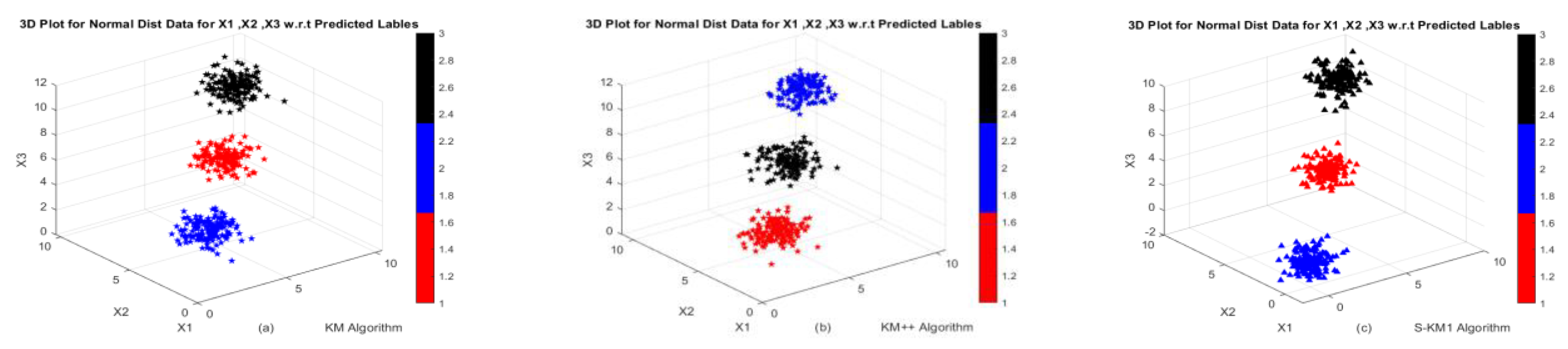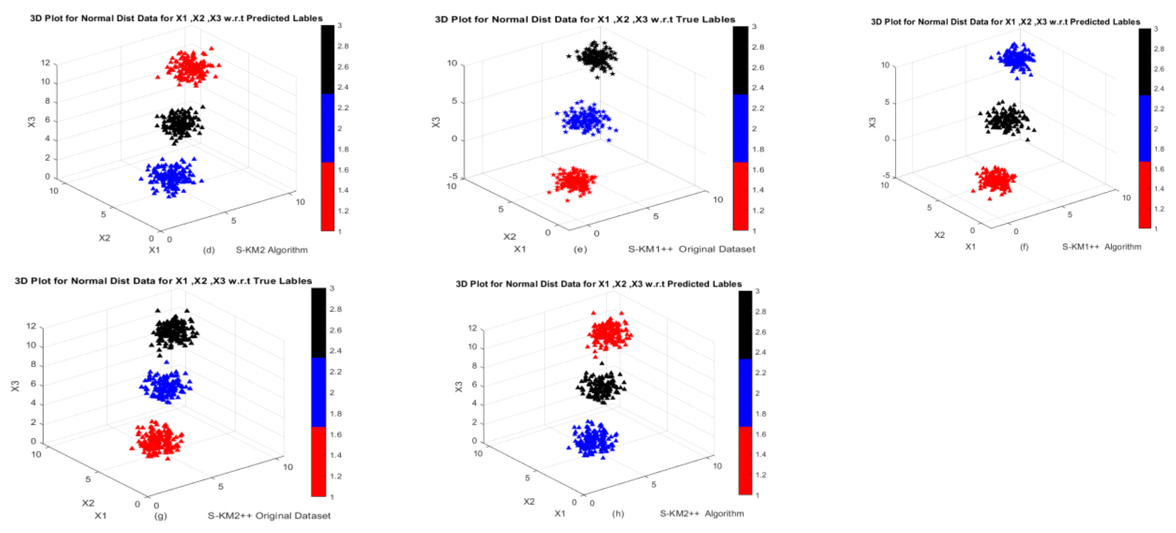The clustering structures show in Figure 2 w.r.t actual and predicted labels. The clustering performance of k-means, k-means++, existing S-KM1, S-KM2 and proposed Lasso-KM1++, Lasso-KM2++ algorithms is shown in Figure 2a–d w.r.t predicted labels and Figure 2e–h are w.r.t true and predicted labels. The clustering structures indicate that our proposed Lasso-KM1++ and Lasso-KM2++ effectively identify meaningful clusters.

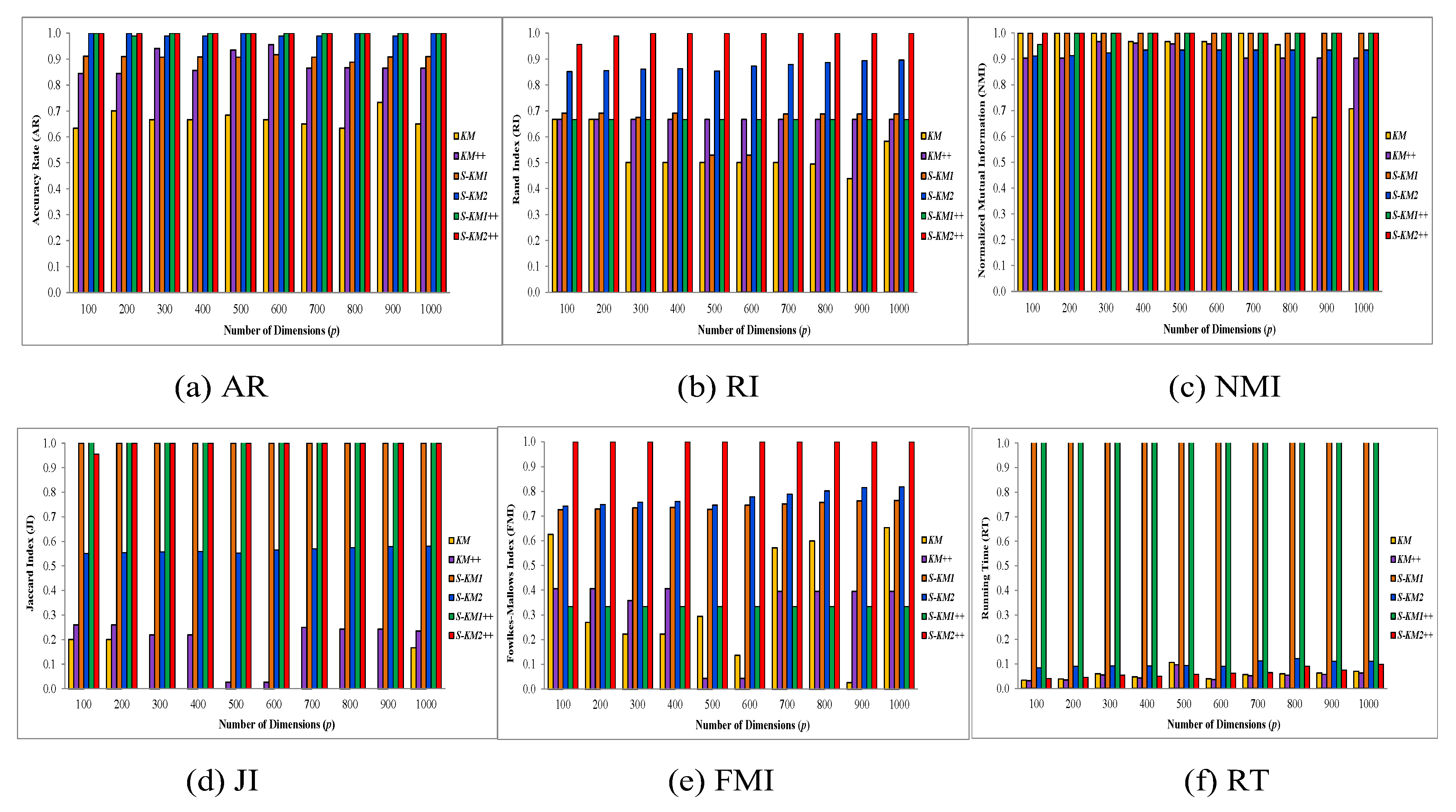
Example 2.

(Using different dimensions, continue with Example 1) We continue with generating the datasets in Example 1. Let $X_{n\times p}$ be the generated data matrix in this experiment with four clusters $C_1,\dots ,C_4$ based on the four normal distributions with means $-\mu ,0,\mu ,2\mu$ in the first q features, respectively. Moreover, for the rest of $\left(p-q\right)$ features, it has mean $\mu =0$ using a similar normal distribution. We generated data points with different dimensions, i.e., $p=100$ to $p=1000$ with fixed or specified mean value $\mu =2.5$ in this experiment. In this study, we evaluated the clustering performance of our proposed Lasso-KM1++ and Lasso-KM2++ algorithms and compared them with traditional KM, KM++, and existing S-KM1, and S-KM2 algorithms under different feature dimensions from $p=100,\dots ,1000$. The six algorithms are compared in Figure 3 using average AR, RI, NMI, JI, FMI and RT as bar graphs. On the basis of performance evaluations by AR, RI, NMI, JI, FMI and RT, we demonstrated that the proposed Lasso-KM2++algorithm outperformed the k-means, k-means++, S-KM1, and S-KM2 algorithms. In addition, results show that Lasso-KM2++ runs much quicker than Lasso-KM1++ and is even faster than the existing S-KM1 and S-KM2 algorithms. Ultimately, due to the use of gap statistics for the tuning parameter, Lasso-KM1++ requires longer to complete the clustering process. To sum up, the recommended Lasso-KM2++ method surpasses the k-means, k-means++, S-KM1, S-KM2, and proposed Lasso-KM1++ algorithms.

Example 3.

(Increasing sample size n = 100…1000) We continue generating the datasets by using the way in Example 1. In this experiment, let the data matrix be $X_{n\times p}$ with three clusters $C_1,C_2,C_3$ generated by the three normal distributions with means $\left\{-\mu ,0,\mu \right\}$ for the initial $q=25$ features. Further, the rest of the $\left(p-q\right)$ features were generated with $\mu =0$ mean. The mean value is specified $\mu =3.0$ to generate the datasets with increasing sample sizes of data points from $n=100,\dots ,1000$ to with specified feature dimension $p=1000$ and $q=25$. We evaluated the performance of the k-means, k-means++, S-KM1, and S-KM2 and the efficiency and strength of our proposed Lasso-KM1++, and Lasso-KM2++ clustering algorithms. Moreover, there are 100 simulations for these generated data points under different sample sizes on different initials and the results are shown in

Table 2. The average measures AR, JI, RI, NMI, FMI and RT for k-means, k-means++, S-KM1, S-KM2, Lasso-KM1++, and Lasso-KM2++ algorithms.

Algorithms	Evaluation Measures
	AR	RI	NMI	JI	FMI	RT
k-means	0.9990	0.5549	0.9838	0.2000	0.3323	0.0703
k-means++	0.9990	0.9987	0.9876	0.9862	0.9980	0.0628
S-KM1	0.9990	0.9620	0.9058	0.9093	0.9429	3.1512
S-KM2	0.9995	0.6657	0.6253	0.3136	0.4775	0.0796
Lasso-KM1++	0.9990	0.9993	0.9938	0.9980	0.9990	0.0881
Lasso-KM2++	1.0000	1.0000	1.0000	1.0000	1.0000	0.0787

Note: Boldface represents the best; Underline represents the second best.

.

Furthermore, results show that both of our proposed Lasso-KM1++ and Lasso-KM2++ algorithms perform superior based on average AR, RI, NMI, JI and FMI over the k-means, k-means++, S-KM1, S-KM2 algorithms. In Table 2, the results show that our proposed S-KM2++ algorithm outperforms the k-means, k-means++, S-KM1, S-KM2 and proposed Lasso-KM1++ algorithm based on average AR, RI, NMI, JI and FMI. Moreover, KM and KM++ have the lowest total running time RT (0.0628, 0.0703) but the proposed Lasso-KM2++ has a minimum average total running time RT as well (0.0787) as well. The clustering structures show in Figure 3 w.r.t. actual and predicted labels. The clustering performance of k-means, k-means++, S-KM1, S-KM2 and proposed Lasso-KM1++, Lasso-KM2++ algorithms is displayed in Figure 2a–d w.r.t predicted labels and 2e–h are w.r.t true and predicted labels. The clustering structures illustrate the superb powers of our proposed Lasso-KM1++ and Lasso-KM2++ algorithms for effective clustering structures. Therefore, we concluded that the proposed Lasso-KM2++ shows superior performance compared to all other competing algorithms. Figure 4a–d show the performance of k-means, k-means++, S-KM1 and S-KM2 based on the predicted labeling, while Figure 4e,g are just the original dataset based on ground truth labeling and Figure 4f,h show the performance of our proposed Lasso-KM1++ and Lasoo-KM2++ algorithms based on predicted labeling. The minor variations in axis scaling across 3D plots result from MATLAB’s automatic axis adjustment when rotating figures for better visualization. Despite these visual differences, the underlying data range remains consistently between −5 and 5 in all figures and similar for the other figures.

Example 4.

(Gaussian mixture distributed data matrix) Let $X=\left\{x_1,x_2,\dots ,x_n\right\}$ be the data points generated by using Gaussian mixture distribution with ${\displaystyle {\sum }_{z=1}^3{\alpha }_{z}N\left({\mu }_z,{\Sigma }_z\right)}$. In this experiment, the Gaussian distributed dataset is generated with the mean vectors ${\mu }_1={[3,3,3]}^T,{\mu }_2={[6,6,6]}^T,{\mu }_3={[9,9,9]}^T$ and ${\alpha }_z=1/3,z=1,2,3$ with ${\Sigma }_z=0.30I;z=1,2,3$ variance covariance matrices, where identity matrix is denoted by I. We generated three clusters $C_1,C_2,C_3$ of synthetic datasets, and the members of data points are n = 450 with number of features p = 15. The dataset was generated by the Gaussian mixture distribution, and has three relevant features; the number of total features is fifteen (15) and the rest of twelve (12) features are generated from uniform distribution with $\mu =0$ mean. We applied our proposed Lasso-KM1++ and Lasso-KM2++ algorithms and made a comparison with k-means, k-means++, S-KM1, and S-KM2 clustering algorithms on this synthetic data to show their effectiveness and strength.

Based on average AR, RI, NMI, JI, FMI and RT, the performance of our proposed LASSO-KM1++, S-KM2++ algorithms is shown in

Table 3. The average-based measures AR, JI, RI, NMI, FMI and RT for k-means, k-means++, S-KM1, S-KM2, Lasso-KM1++, and Lasso-KM2++ algorithms.

Algorithms	Evaluation Measures
	AR	RI	NMI	JI	FMI	RT
k-means	0.9565	0.5570	0.9898	0.2016	0.3356	0.0439
k-means++	0.9992	0.5733	0.9883	0.2195	0.3600	0.0394
S-KM1	0.9999	0.5733	0.9998	0.2897	0.5733	2.4379
S-KM2	1.0000	0.9957	1.0000	0.9991	0.9874	0.0175
Lasso-KM1++	0.9833	0.5733	0.9394	0.9672	0.9833	2.0182
Lasso-KM2++	1.0000	0.9962	1.0000	0.9994	0.9883	0.0158

Note: Boldface represents the best; Underline represents the second best.

. In Table 3, the values that rank highest are shown in bold, while the values that rank next are underlined. From Table 3, the results demonstrate that our proposed Lasso-KM2++ algorithm shows superiority under average measures of AR, RI, NMI, JI, FMI and RT. In addition, the average total running time (RT) of the Lasso-KM2++ algorithm with 0.0158 (sec.) is even faster than the existing S-KM2 algorithm with 0.0175 (sec.). In summary, the proposed Lasso-KM2++ shows excellent results in this experiment and has good clustering abilities as well. The graphical behavior of both proposed Lasso-KM1++ and Lasso-KM2++ algorithms is shown in Figure 5e–h.

3.2. Evaluation and Comparison with Real Datasets

Based on the UCI machine learning repository and Kaggle datasets [49,50], we analyze the effectiveness and efficiency of our proposed Lasso-KM1++, and Lasso-KM2++ algorithms by numerous real datasets. Numerous datasets that include Breast Cancer, Seeds, Lungs and Red Wine have also been used by researchers and scientists in various fields. These real datasets were used to test, compare, and evaluate the effectiveness and competence of our proposed Lasso-KM1++ and Lasso-KM2++ algorithms for relevant feature selection as well. We conduct 100 simulations of clustering results based on various seed values. Furthermore, we also show the feature selection competency of both the proposed Lasso-KM1++ and Lasso-KM2++ algorithms. We initialize feature weights that generate sparse features using the lasso penalty term so that it can discard the irrelevant features towards exactly zero and select the relevant features as well.

Example 5.

(Iris dataset) In this experiment, we show the performance of our proposed algorithms by using a real iris dataset [49]. In the field of machine learning and statistics, the Iris dataset is a well-known dataset for demonstrating and testing various data analyses and machine learning algorithms. In 1936, British biologist and statistician Ronald A. Fisher introduced the concept of multiple measurements in taxonomy. The iris dataset has 150 data points and four features namely PL (petal length), PW (petal width), SL (sepal length), and SW (sepal width), and there are three different species of iris: Iris versicolor, Iris virginica, and Iris Setosa. The number of features is p = 4 with initialized weights $w_j=1/\sqrt{p}$ and we set the value of the tuning parameter $\lambda =1.2$ that generates sparsity (significant number of zero or near-zero values). The top-ranked values are presented in bold in

Table 4. (A) The average performance of AR, JI, RI, NMI, FMI and RT for KM, KM++ in Example 5. (B) The average performance of AR, JI, RI, NMI, FMI and RT for S-KM1, Lasso-KM1++ in Example 5. (C) The average performance of AR, JI, RI, NMI, FMI and RT for S-KM2, Lasso-KM2++ in Example 5. (D) The average performance of AR, JI, RI, NMI, FMI and RT for S-KM1, Lasso-KM1++ in Example 5. (E) Final feature weights.

Algorithm	Performance Measures
	AR	RI	NMI	JI		FMI		RT
(A)
k-means	0.8867	0.4933	0.7419	0.1364		0.2400		0.0084
k-means++	0.9000	0.6222	0.7981	0.2766		0.4333		0.0044
(B)
S-KM1	0.9700	0.9289	0.7433	0.8072		0.8933		1.3501
Lasso-KM1++	0.9993	0.9289	0.8642	0.8072		0.8933		1.2288
(C)
S-KM2	0.9733	0.9700	0.8642	0.9231		0.9550		0.0654
Lasso-KM2++	0.9997	0.9733	0.8642	0.9231		0.9600		0.0396
(D)
k-means++	0.9000	0.6222	0.7981	0.2766		0.4333		0.0044
Lasso-KM1++	0.9993	0.9289	0.8642	0.8072		0.8933		1.2288
Lasso-KM2++	0.9997	0.9733	0.8642	0.9231		0.9600		0.0396
(E)
Algorithms	Feature Weights
	PL		PW		SL		SW
Lasso-KM1++	0.0000		0.2353		0.6276		0.0000
Lasso-KM2++	0.0000		0.0820		0.1311		0.3662

Note: Boldface represents the best; Underline represents the second best.

, while the second-ranked values are underlined. The results show the effectiveness, efficiency and strength of both of our proposed Lasso-KM1++ and Lasso-KM2++ algorithms given below. The performance of existing and proposed algorithms is shown in Table 4A–E which is provided. The results demonstrated the superiority of our proposed Lasso-KM1++ and S Lasso-KM2++ algorithms based on average (AR, RI, FMI and RT) over all the other competing algorithms, e.g., k-means, k-means++, S-KM1, and S-KM2.

The results in Table 4A show the superiority of k-means++ over traditional k-means in terms of all measures used in this experiment. For the average total running time RT (in sec.) the KM++ is the fastest with 0.0044. In

Table 5. The average measures AR, JI, RI, NMI, FMI and RT for KM, KM++, S-KM1, S-KM2, Lasso-KM1++, Lasso-KM2++ algorithms.

Algorithms	Performance Measures
	AR	RI	NMI	JI	FMI	RT
k-means	0.8867	0.5888	0.4990	0.7337	0.1923	0.0087
k-means++	0.9886	0.6216	0.8444	0.4762	0.1571	0.0083
S-KM1	0.9760	0.5888	0.8274	0.4049	0.7411	2.8866
S-KM2	0.9732	0.5972	0.8317	0.4233	0.7476	0.0242
Lasso-KM1++	0.9720	0.5220	0.7410	0.5680	0.7000	0.0781
Lasso-KM2++	0.9999	0.8254	0.8354	0.5849	0.7481	0.0078

Note: Boldface represents the best; Underline represents the second best.

the proposed Lasso-KM1++ surpasses existing S-KM1 based on average AR, and NMI where RI, JI and FMI are the same. The RT (in sec.) of the Lasso-KM1++ is the fastest with 1.2288 which is smaller than the existing S-KM1 algorithm. The results in Table 4C show that our proposed Lasso-KM2++ algorithm is superior based on average AR, RI, and FMI but the same for NMI, and JI. The proposed Lasso-KM2++ algorithm is fast as well with minimum total running time (RT) that is 0.0396. The total running time RT of the existing S-KM1 and proposed Lasso-KM1++ algorithms is the slowest due to the use of gap statistics. Table 4D shows that the proposed Lasso-KM2++ algorithm surpasses over existing S-KM2 in terms of average AR, RI, JI, and FMI but NMI remains the same. The proposed Lasso-KM2++ method shows excellent results in k-means and k-means++ algorithms as well. The total average running time RT for k-means++ is minimum but the RT of our Lasso-KM2++ method is minimum as well. The non-zero weights for feature selection ability are also shown in Table 4E. Both proposed Lasso-KM1++ and Lasso-KM2++ methods discarded the irrelevant features and shrunk them towards exactly zero, gaining the advantage of the Lasso penalty term. The efficiency and excellent performance show that the proposed Lasso-KM2++ algorithm beats all the other competing algorithms in terms of different clustering measures. Both Lasso-KM1++ and Lasso-KM2++ have excellent clustering performance based on feature selection behavior in Table 4A–E and good clustering structures in Figure 6e–h.

In addition, we evaluated the performance of S-KM1 and our proposed Lasso-KM1++ algorithms by using another performance measure that is the standard deviation (SD) of our six evaluation performance measures of AR, RI, NMI, JI, FMI, RT by using different initials. We obtain the corresponding values for SDs of algorithms: $4.47\times {10}^{-5}, 0.0028, 0.0038, 0.0059, 0.0036, 0.2266 \&$$4.33\times {10}^{-5}, 0.0024, 0.0036, 0.0057,$ $0.0035, 0.1329,$ respectively. Furthermore, we also analyzed the performance effectiveness of another S-KM2 algorithm and our proposed Lasso-KM2++ algorithm based on similar performance measures of SDs with the corresponding results shown as $0, 2.30\times {10}^{-16}, 2.29\times {10}^{-16}, 1.15\times {10}^{-16}, 4.60\times {10}^{-16}, 0.0207$ and $2.22\times {10}^{-16}, 0, 2.29{\times 10}^{-16}, 1.14\times {10}^{-16},$ $4.44\times {10}^{-16},0.0203$, respectively. The SD values of AR with $2.22\times {10}^{-16}$ for Lasso-KM2++ are extremely low, meaning the accuracy rate is very stable across different initial seeds. RI with 0 means “perfect stability”; NMI with $2.29\times {10}^{-16}$ means “very small deviation”, indicating consistent NMI, and so forth. Similarly, the SD values for the k-means and k-means++ algorithms are $0.1363, 0.1978, 0.0566, 0.2727, 0.2866, 0.0025 \&$ $0.1183, 0.1773, 0.0608, 0.2419, 0.2456, 0.0007$, respectively.

Example 6.

(The SEEDS dataset). The Seeds dataset [49] has seven geometric features of the wheat kernel that are extracted from images. In agricultural research and pattern recognition, the Seeds dataset is a well-known dataset for classification and clustering. Its size of data points is 120 with seven features namely, Area A, Perimeter P, Compactness, Length of Kernel and Width of Kernel, Asymmetry Coefficient, and Kernel Groove Length. It was classified into three different varieties of wheat (Kama, Rosa and Canadian). In addition, in order to evaluate the performance of Lasso-KM1++ and Lasso-KM2++ algorithms as well as examine their feature selection capability, we applied these algorithms to these real-world datasets. The performance of proposed Lasso-KM1++, and Lasso-KM2++ algorithms and their comparisons with traditional KM, KM++and existing S-KM1, and S-KM2 algorithms are shown in Table 5. The results in Table 5 show that the proposed Lasso-KM1++, and Lasso-KM2++ algorithms surpass all the competing algorithms based on six evaluation measures, where bold represents the best value and underline indicates the second-best value.

In accordance with average accuracy (AR), the results in Table 5 demonstrate that our proposed Lasso-KM2++ algorithms outperform existing S-KM1 and S-KM2 and traditional KM, KM++algorithms for the Seeds dataset. However, both the proposed Lasso-KM1++ and the existing S-KM1 algorithm require more computational work and time. Based on AR, RI and FMI and total running time (RT), the Lasso-KM2++ algorithm demonstrated better performance than the traditional KM, KM++ and existing S-KM1 and S-KM2 algorithms. On the basis of total running time (RT), the recommended Lasso-KM2++ algorithm appears to be quick and easy despite the fact that the conventional KM and KM++ algorithms are always the quickest in RT. In general, Lasso-KM2++ surpasses all the other competing algorithms.

Example 7.

(The RED WINE dataset) The Red Wine Quality Dataset [50] is a well-known dataset that is often used for classification and regression tasks. The red wine dataset, which has 1599 data points and total number of features 12 (fixed acidity, volatile acidity, citric acid, residual sugar, chlorides, free sulfur dioxide, total sulfur dioxide, density, pH, sulphates, alcohol, and quality), is a collection of chemical and sensory data about red wine. We use this dataset to apply our proposed Lasso-KM1++ and Lasso-KM2++ and compare them with these competing clustering algorithms, such as KM, KM++, S-KM1 and S-KM2. Following an algorithmic comparison,

Table 6. The average measures AR, JI, RI, NMI, FMI and RT for KM, KM++, S-KM1, S-KM2, Lasso-KM1++, Lasso-KM2++ algorithms.

Algorithms	Performance Measures
	AR	RI	NMI	JI	FMI	RT
k-means	0.8968	0.0418	0.0413	0.0000	0.0000	0.0214
k-means++	0.9980	0.6646	0.0409	0.0000	0.0000	0.0199
S-KM1	0.9875	0.0187	0.5295	0.0409	0.0394	2.9880
S-KM2	0.9999	0.0095	0.5208	0.0371	0.0203	0.0442
Lasso-KM1++	0.9999	0.6646	0.0418	0.0000	0.0000	2.0892
Lasso-KM2++	1.0000	0.6646	0.0418	0.0418	0.0000	0.0202

Note: Boldface represents the best; Underline represents the second best.

displays the performance results of the proposed Lasso-KM1++and Lasso-KM2++algorithms:

The results in Table 6 show that our both proposed Lasso-KM1++ and Lasso-KM2++ algorithms performed well over traditional KM, KM++ and existing S-KM1 and S-KM2 for Red Wine datasets based on average accuracy (AR) but both the existing S-KM1 and the proposed Lasso-KM1++ algorithm are more complicated in computational work and these algorithms are time-consuming as well based on total running time RT. We concluded that both proposed Lasso-KM1++ and Lasso-KM2++ algorithms demonstrated better performance than the traditional KM, KM++ and existing S-KM1 and S-KM2 algorithms based on average accuracy (AR) and total running time (RT). However, the traditional KM and KM++ algorithms have a minimum total running time (RT) but the proposed Lasso-KM2++ algorithm has a minimum total running time (RT). In general, Lasso-KM2++ surpasses all the other competing algorithms. The results in

Table 7. Feature selection performance of our proposed Lasso-KM1++ and Lasso-KM2++ clustering algorithms.

DATASETS	Data Point n	No. of Features p	No. of Clusters c	Non-Zero Feature Weights
				Lasso-KM1++	Lasso-KM2++
Seeds	210	7	3	4	2
Iris	150	4	3	3	3
Red wine	1599	12	6	5	5

illustrate how the Lasso-KM1++ and Lasso-KM2++ algorithms select features (the number of relevant features with nonzero weights). We concluded that both Lasso-KM1++ and Lasso-KM2++ algorithms have good clustering results and feature-selection ability as well as shown in Table 5, Table 6 and Table 7. In summary, we recommend using Lasso-KM2++ in clustering due to its performance, running time, and feature selection.

We next make more comparative analysis among these compared clustering algorithms. In total, the computational cost of Lasso-KM2++ is lower than S-KM, S-KM1, S-KM2 and SPCM because S-KM and S-KM1 are based on gap statistics, which are more complicated and time-consuming, and SPCM2 has more parameters in consideration. The Lasso-KM2++ algorithm boosts clustering efficiency and integrates enhanced centroid initialization with feature-based sparsity for high-dimensional datasets. To improve clustering stability and reduce sensitivity to random initialization, Lasso-KM2++ applies KM++ initialization, which consciously selects centroids. The Lasso-KM2++ algorithm boosts clustering performance by promoting sparsity with optimized centroid initialization, making it highly relevant for high-dimensional data analysis and ensuring better cluster stability and robustness against poor local optima. In addition, Lasso-KM2++ balances the trade-off between sparsity and cluster quality, ensuring that essential features are retained without compromising accuracy. We summarize the superiority of Lasso-KM2++ and its beneficial applications as follows: (1) Effective Feature Selection in High-Dimensional Data: In datasets with many irrelevant or redundant features, k-means struggles due to the curse of dimensionality. Lasso-KM2++ applies sparsity constraints, ensuring that only the most relevant features contribute to clustering, leading to better-defined clusters in high-dimensional datasets with many noisy features. (2) More Stable and Consistent Cluster Assignments: Lasso-KM2++ minimizes variability in results by including Lasso directly into the objective function, which ensures that the clustering process determines the most informative features. (3) Robustness to Noisy Features and Outliers: Lasso-KM2++ automatically eliminates less informative features. This makes it robust to datasets with high levels of noise, similar to those found in social networks or sensor data analysis. (4) Improved Interpretability and Computational Efficiency: Lasso-KM2++ makes the clustering results easier to understand by reducing the number of active features with the application of sparsity. In large-scale data cases where computational efficiency is an issue, Lasso-KM2++ is especially beneficial due to feature reduction, which additionally decreases computational complexity.

4. Conclusions

In this paper, we introduce the Lasso-KM1++ and Lasso-KM2++ clustering algorithms, designed to efficiently handle high-dimensional datasets by integrating Lasso regularization with the k-means++ initialization technique. These algorithms effectively eliminate irrelevant features while preserving the most informative ones, enhancing both clustering accuracy and interpretability. They ensure a more meaningful feature selection process by using Lasso regularization to give nonzero weights to essential features and zero weights to unnecessary ones. The proposed Lasso-KM1++ and Lasso-KM2++ are effective tools for sparse clustering in high-dimensional spaces since they embed the good k-means++ initialization technique, which speeds up computation and enhances clustering robustness. Furthermore, we analyzed the performance of the Lasso-KM1++ and Lasso-KM2++ clustering algorithms and compared them with k-means, k-means++, S-KM1, and S-KM2. The evaluation is based on the average performance measures, including AR, RI, NMI, JI, FMI, and RT, providing a comprehensive assessment of their effectiveness. In particular, the proposed Lasso-KM2++ algorithm achieves superior results by directly incorporating the Lasso penalty into its objective function for efficient feature selection while benefiting robust cluster initialization. In contrast, Lasso-KM1++ is more complex and computationally demanding due to the use of gap statistics. The Lasso penalty is directly integrated into the objective function of Lasso-KM2++, which leads to more accurate and efficient feature selection compared to S-KM, which achieves it indirectly. In contrast to SPCM, the proposed Lasso-KM2++ algorithm demonstrates superiority as SPCM involves more parameters, which may further increase computational complexity and time consumption. The Lasso-KM2++ algorithm benefits from k-means++ initialization, which places centroids more strategically, reducing the risk of local optima and enhancing clustering accuracy. This results in faster convergence, enhanced robustness, and greater stability, making it more efficient and reliable compared to algorithms such as k-means, k-means++, S-KM, and SPCM. The results and figures demonstrate that both proposed Lasso-KM1 and Lasso-KM2 present better results and clustering structures. On the basis of comparison and performance, it is evident that the proposed Lasso-KM2++ algorithm is simple to understand, time-efficient, and easy to implement. On the other hand, the results demonstrate that the proposed Lasso-KM2++ algorithm performs better on both artificial and real datasets by providing good clustering results as well. Based on the total average running time (RT) criterion, the Lasso-KM2++ algorithm provides the most outstanding performance. The appealing feature of the S-KM2 algorithm is that it chooses the relevant features and assigns them non-zero weights while it discards the irrelevant features and shrinks them towards exactly zero. Although the proposed Lasso-KM++ algorithms apply Lasso to enforce sparsity and use KM++ initialization for well-handling high-dimensional datasets, they rely on Euclidean distances. This makes Lasso-KM++ limited; it assumes spherical clusters and makes them less effective for irregular cluster structures. Another limitation is it becomes highly sensitive to noisy points and outliers. Improving these limitations of Lasso-KM++ will be our further research topic. On the other hand, we know that SPCM suffers from mode-seeking behavior, meaning it can form small, dense clusters without proper separation and also parameter initialization problems. Based on the idea in Lasso-KM++, we may try to help SPCM in improving mode-seeking and parameter initialization problems in the future. In addition, we will further extend the Lasso-KM++ algorithms for clustering multi-view datasets.