
Mapping the Past: Unlocking Historical Explorer Narratives with AI and Geospatial Tools

Abstract
1. Introduction
1.1. Explorer Accounts as Historical Sources
1.2. Challenges and Limitations of Traditional Analysis
1.3. Contributions of Quantitative and Computational Approaches
1.4. Objectives and Hypothesis
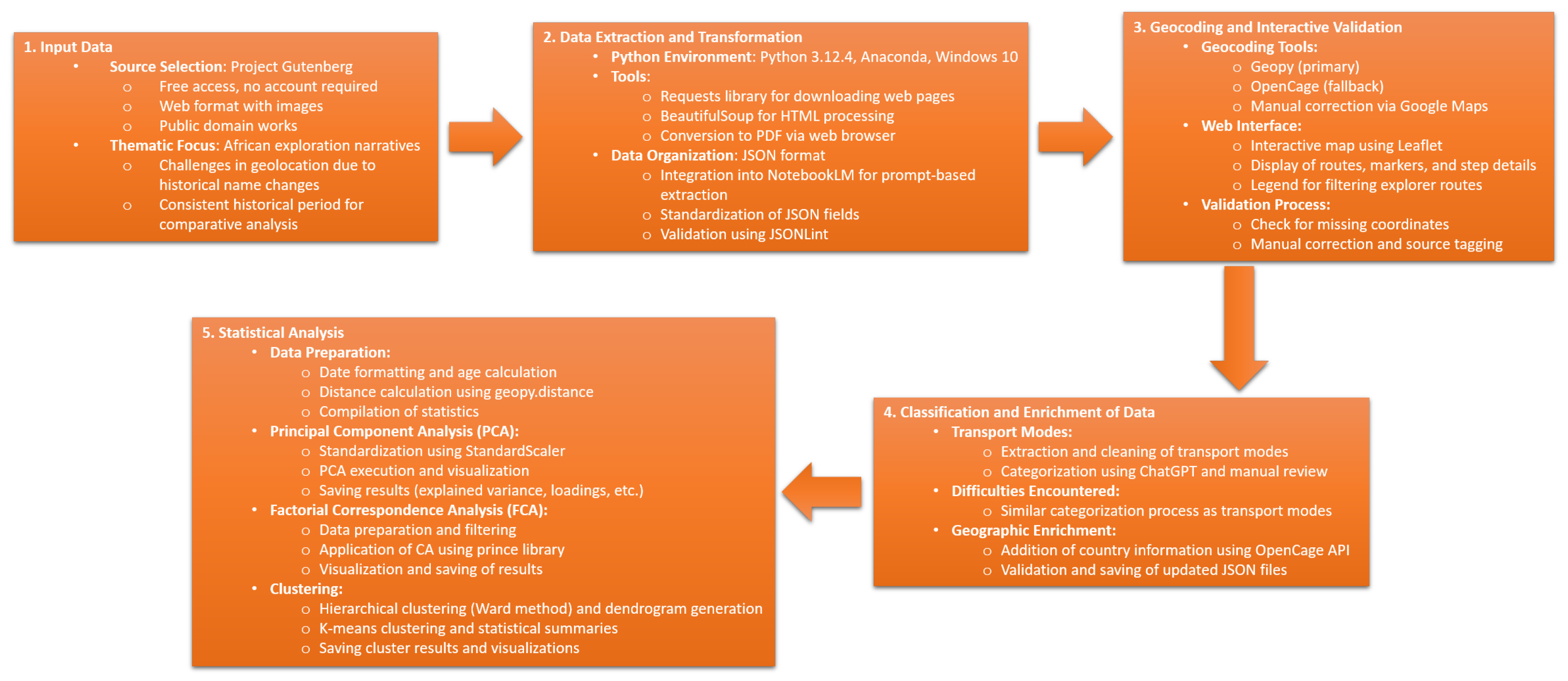
2. Materials and Methods
2.1. Input Data
2.2. Data Extraction and Transformartion
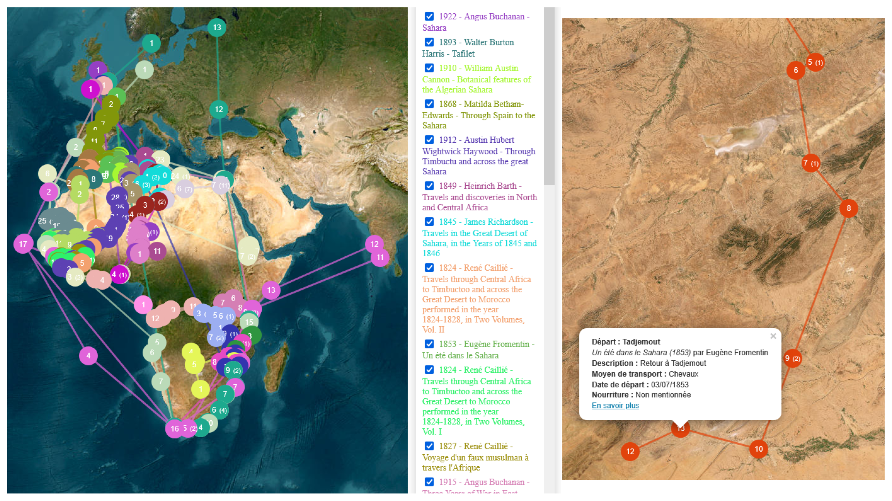
2.2.1. Geocoding and Interactive Validation
2.2.2. Classification and Enrichment of Data
2.3. Statistical Analysis
2.3.1. Principal Component Analysis
2.3.2. Factorial Correspondence Analysis
2.3.3. Clustering
3. Results
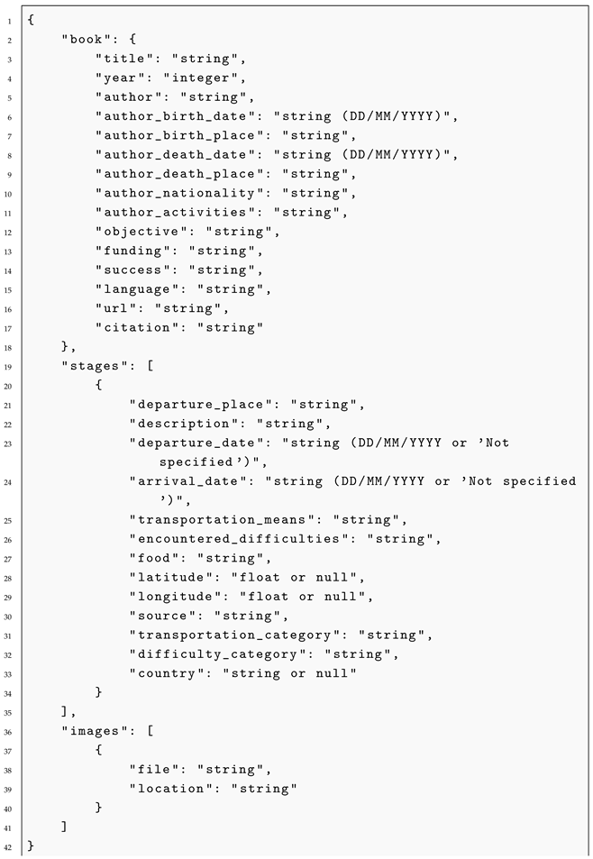
| Listing 1. JSON schema for documenting exploration narratives |
 |
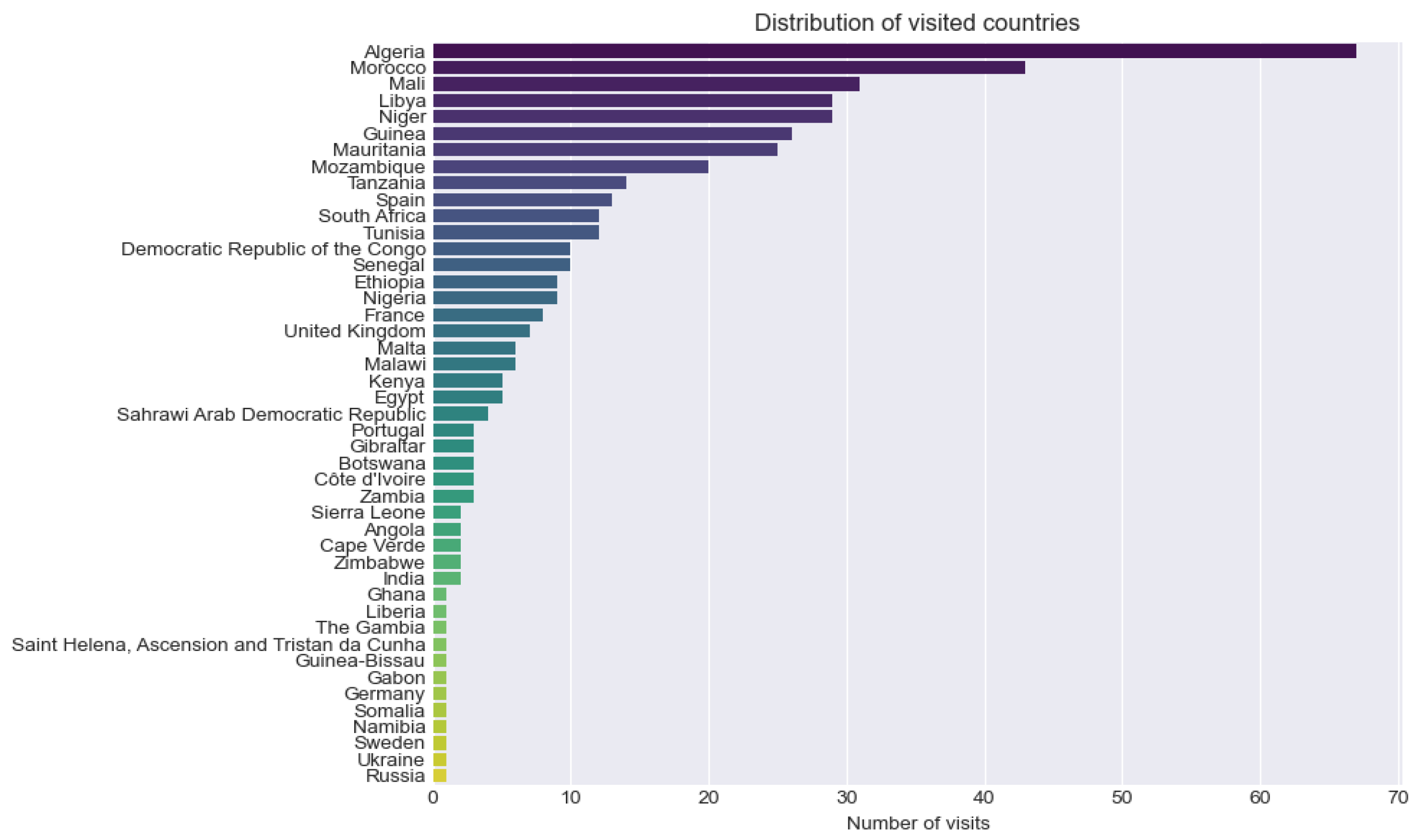
3.1. Travel Metrics
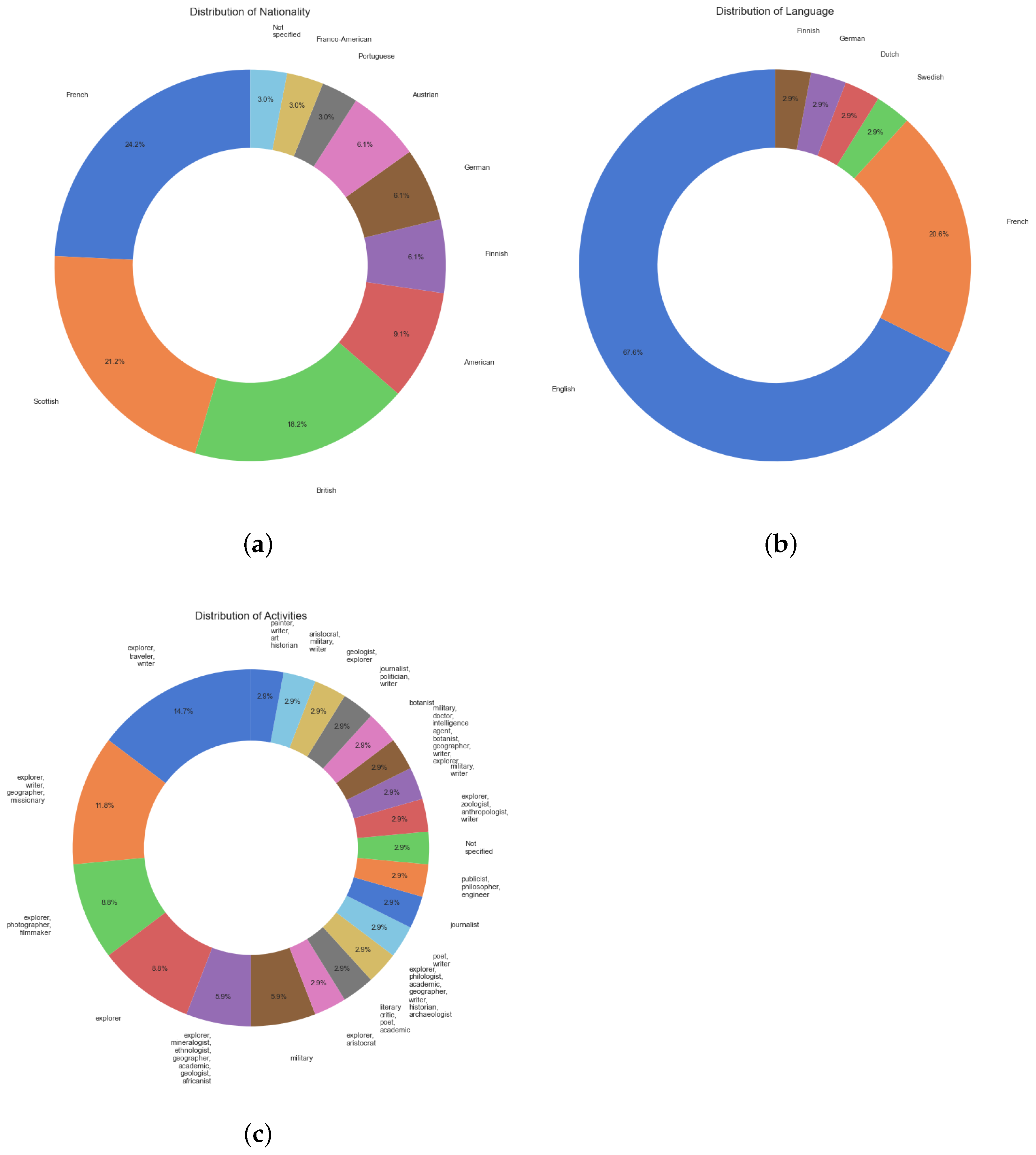
3.2. Author Metrics
3.3. Principal Component Analysis
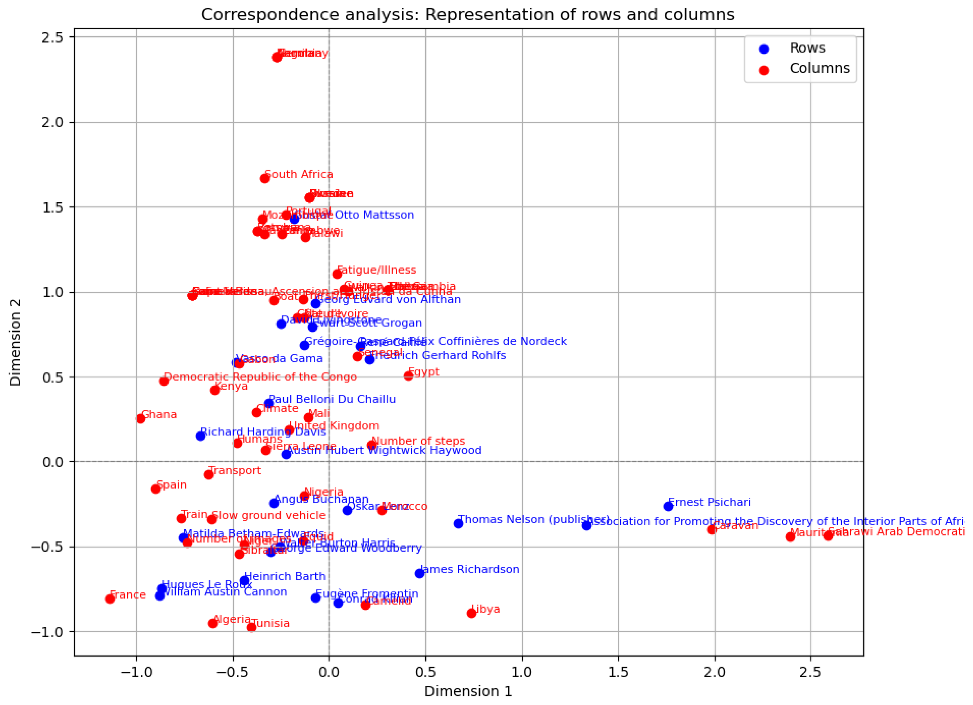
3.3.1. Correspondence Factor Analysis
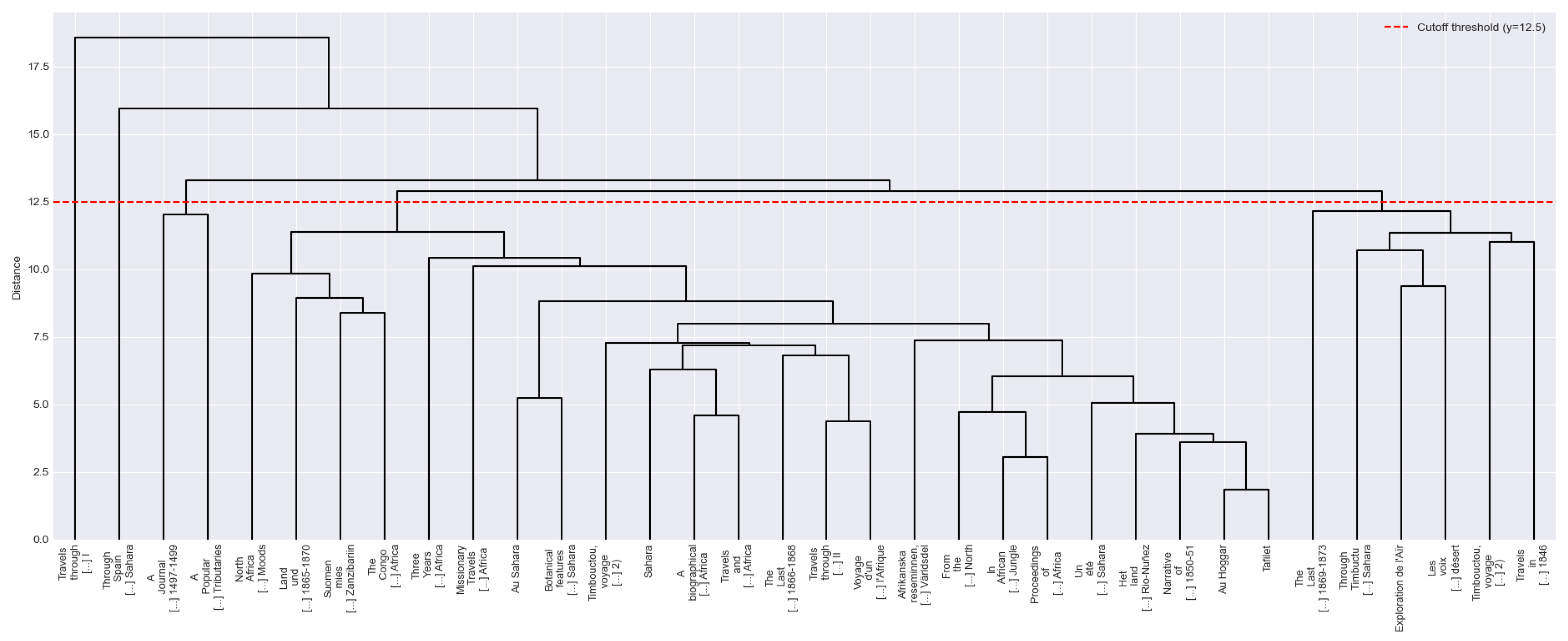
3.3.2. Clustering
4. Discussion
4.1. Methodological Contributions
4.2. Corpus Structuring
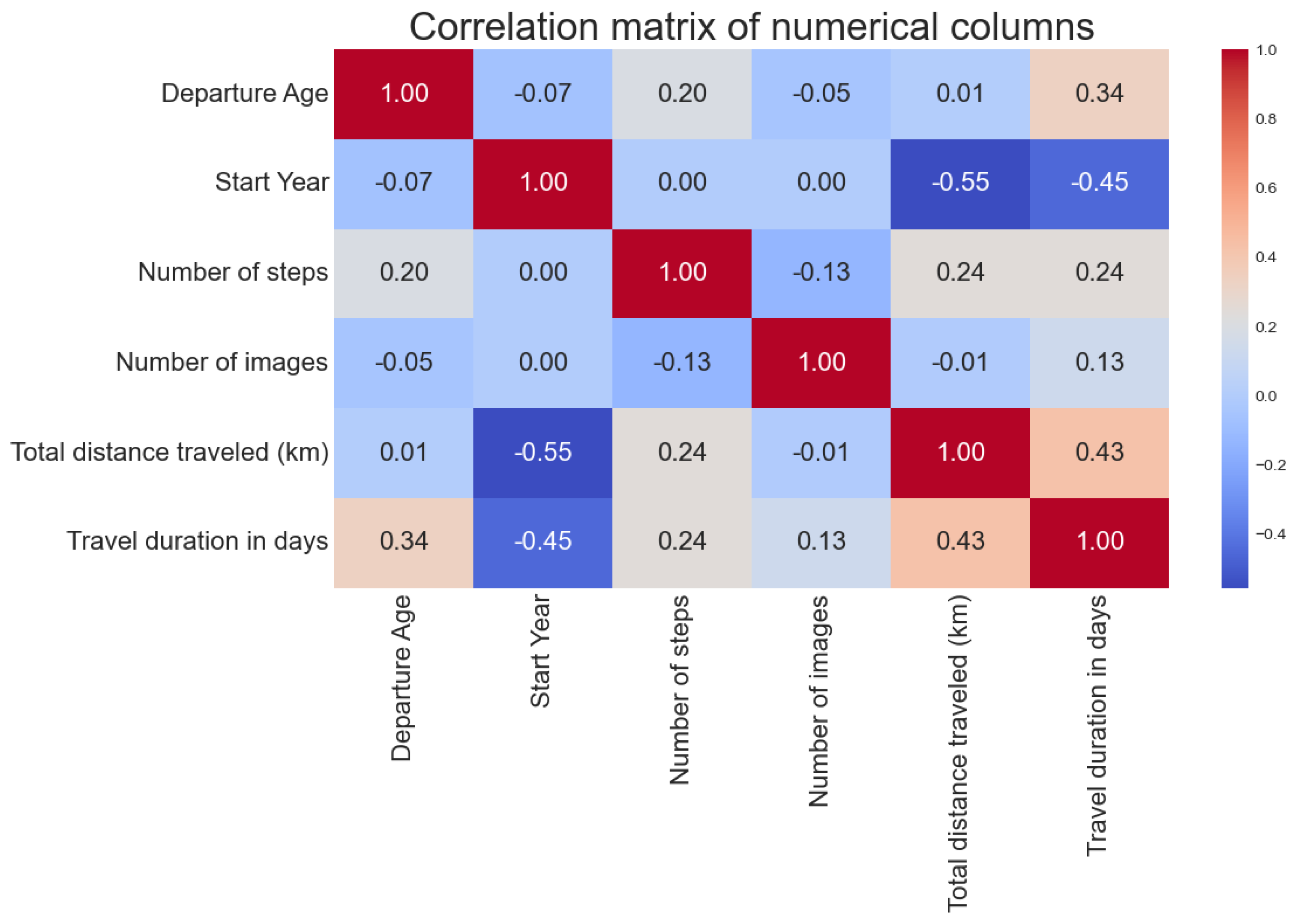
4.3. Correlation Analysis
4.4. Influence of External Factors
4.5. Empirical Validation and Historiographical Enrichment
4.6. Methodological Limitations and Biases
4.7. Future Perspectives
5. Conclusions
Funding
Institutional Review Board Statement
Informed Consent Statement
Data Availability Statement
Conflicts of Interest
References
- Yves, B. Explorations en Afrique centrale, 1790–1930: Apport des explorateurs à la connaissance du milieu. J. Afr. 2024, 93, 413–414. [Google Scholar]
- Holtz, G.; Masse, V. Étudier les récits de voyage: Bilan, questionnements, enjeux. Arborescences 2012. [Google Scholar] [CrossRef]
- Lefebvre, C. Chapitre I. Dans les pas des explorateurs. In Frontières de Sable, Frontières de Papier; Éditions de la Sorbonne: Paris, France, 2015. [Google Scholar]
- Gauthier, J. La Société de géographie commerciale de Bordeaux: Sur les traces des explorateurs entre 1874 et 1911. Dyn. Environ. J. Int. Géosci. L’Environ. 2017, 39–40, 36–53. [Google Scholar] [CrossRef]
- Gallou-Guyot, M.; Rousseau, C.; Perrochon, A. Les limites des revues systématiques de la littérature–quand le trop d’information devient délétère. Kinésithér. Rev. 2024, 24, 60–65. [Google Scholar]
- Roetzel, P.G. Information overload in the information age: A review of the literature from business administration, business psychology, and related disciplines with a bibliometric approach and framework development. Bus. Res. 2019, 12, 479–522. [Google Scholar] [CrossRef]
- Shahrzadi, L.; Mansouri, A.; Alavi, M.; Shabani, A. Causes, consequences, and strategies to deal with information overload: A scoping review. Int. J. Inf. Manag. Data Insights 2024, 4, 100261. [Google Scholar] [CrossRef]
- Seutter, J.; Kutzner, K.; Stadtländer, M.; Kundisch, D.; Knackstedt, R. “Sorry, too much information”—Designing online review systems that support information search and processing. Electron. Mark. 2023, 33, 47. [Google Scholar]
- Rörden, J.; Gruber, D.; Krickl, M.; Haslhofer, B. Identifying historical travelogues in large text corpora using machine learning. In Sustainable Digital Communities, Proceedings of the 15th International Conference, iConference 2020, Boras, Sweden, 23–26 March 2020; Springer: Cham, Switzerland, 2020; pp. 801–815. [Google Scholar]
- Chachereau, N.; Humair, C. Méthodes informatiques et quantitatives en histoire du tourisme: Apports et limites. Introduction. Mondes Tour. 2023. [Google Scholar] [CrossRef]
- Villamor Martin, M.; Kirsch, D.A.; Prieto-Nañez, F. The promise of machine-learning-driven text analysis techniques for historical research: Topic modeling and word embedding. Manag. Organ. Hist. 2023, 18, 81–96. [Google Scholar] [CrossRef]
- Winterbottom, A.; Bekker, H.L.; Conner, M.; Mooney, A. Does narrative information bias individual’s decision making? A systematic review. Soc. Sci. Med. 2008, 67, 2079–2088. [Google Scholar]
- Betsch, C.; Haase, N.; Renkewitz, F.; Schmid, P. The narrative bias revisited: What drives the biasing influence of narrative information on risk perceptions? Judgm. Decis. Mak. 2015, 10, 241–264. [Google Scholar]
- Partlan, N.; Carstensdottir, E.; Snodgrass, S.; Kleinman, E.; Smith, G.; Harteveld, C.; El-Nasr, M.S. Exploratory automated analysis of structural features of interactive narrative. In Proceedings of the AAAI Conference on Artificial Intelligence and Interactive Digital Entertainment, New Orleans, LA, USA, 2–7 February 2018; Volume 14, pp. 88–94. [Google Scholar]
- Jones, S.; Fox, C.; Gillam, S.; Gillam, R.B. An exploration of automated narrative analysis via machine learning. PLoS ONE 2019, 14, e0224634. [Google Scholar]
- Sudhahar, S.; Cristianini, N. Automated analysis of narrative content for digital humanities. Int. J. Adv. Comput. Sci. 2013, 3, 440–447. [Google Scholar]
- Chen, Q.; Cao, S.; Wang, J.; Cao, N. How does automation shape the process of narrative visualization: A survey of tools. IEEE Trans. Vis. Comput. Graph. 2023, 30, 4429–4448. [Google Scholar] [CrossRef] [PubMed]
- Álvarez-Carmona, M.Á.; Aranda, R.; Rodríguez-Gonzalez, A.Y.; Fajardo-Delgado, D.; Sánchez, M.G.; Pérez-Espinosa, H.; Martínez-Miranda, J.; Guerrero-Rodríguez, R.; Bustio-Martínez, L.; Díaz-Pacheco, Á. Natural language processing applied to tourism research: A systematic review and future research directions. J. King Saud Univ.-Comput. Inf. Sci. 2022, 34, 10125–10144. [Google Scholar]
- Gregoriades, A.; Pampaka, M.; Herodotou, H.; Christodoulou, E. Explaining tourist revisit intention using natural language processing and classification techniques. J. Big Data 2023, 10, 60. [Google Scholar]
- Brunsting, S.; De Sterck, H.; Dolman, R.; van Sprundel, T. Geotexttagger: High-precision location tagging of textual documents using a natural language processing approach. arXiv 2016, arXiv:1601.05893. [Google Scholar]
- Hu, Y.; Mao, H.; McKenzie, G. A natural language processing and geospatial clustering framework for harvesting local place names from geotagged housing advertisements. Int. J. Geogr. Inf. Sci. 2019, 33, 714–738. [Google Scholar]
- Lefebvre, C.; Surun, I. Exploration et transferts de savoir: Deux cartes produites par des Africains au début du 19e siècle. M@ Ppemonde 2008, 4, 1–24. [Google Scholar]
- Lefebvre, C. Frontières de Sable, Frontières de Papier: Histoire de Territoires et de Frontières, du Jihad de Sokoto à la Colonisation Française du Niger, XIXe-XXe Siècles; Éditions de la Sorbonne: Paris, France, 2019. [Google Scholar]
- Buchanan, A. Exploration of Aïr: Out of the World North of Nigeria; J. Murray: South Elgin, IL, USA, 1921. [Google Scholar]
- Buchanan, A. Sahara; J. Murray: South Elgin, IL, USA, 1926. [Google Scholar]
- Buchanan, A. Three Years of War in East Africa; J. Murray: South Elgin, IL, USA, 1920. [Google Scholar]
- Proceedings of the Association for Promoting the Discovery of the Interior Parts of Africa; C. Macrae, Printer to the Association: New York, NY, USA, 1790.
- Haywood, A. Through Timbuctu and across the Great Sahara. Geogr. J. 1913, 41, 278. [Google Scholar]
- Kilian, C. Au Hoggar, Mission de 1922: Ouvrage Orne de Trois Cartes et de Seize Planches Hors-Texte; Société d’éditions géographiques maritimes et coloniales: Paris, France, 1925. [Google Scholar]
- Livingstone, D. A Popular Account of Dr. Livingstone’s Expedition to the Zambesi and Its Tributaries: And of the Discovery of Lakes Shirwa and Nyassa, 1858–1864: Abridged from the Larger Work; J. Murray: South Elgin, IL, USA, 1875. [Google Scholar]
- Livingstone, D. Missionary Travels and Researches in South Africa: In Large Print; BoD–Books on Demand: Norderstedt, Germany, 2022. [Google Scholar]
- Livingstone, D. The Last Journals of David Livingstone: In Central Africa, from 1865 to His Death; RW Bliss: Fort Huachuca, AZ, USA, 1875. [Google Scholar]
- Waller, H. The Last Journals of David Livingstone, in Central Africa; RW Bliss: Fort Huachuca, AZ, USA, 1875. [Google Scholar]
- Psichari, E. Les Voix qui Crient dans le désert: Souvenirs d’Afrique; L. Conard: Washington, DC, USA, 1928. [Google Scholar]
- Fromentin, E. Un été dans le Sahara; Plon: Schleswig-Holstein, Germany, 1888. [Google Scholar]
- Grogan, E.S.; Sharp, A.H. From the Cape to Cairo: The First Traverse of Africa from South to North; Hurst and Blackett: London, UK, 1900. [Google Scholar]
- Rohlfs, G. Land und Volk in Afrika: Berichte aus den Jahren 1865–1870; H. Fischer Nachf: Hamburg, Germany, 1884. [Google Scholar]
- von Alfthan, G.E. Afrikanska Reseminnen: Äfventyr Och Intryck Från en Utflykt Till de Svartes Världsdel; PH Beijer, distr.: Helsingfors, Finland, 1892. [Google Scholar]
- Woodberry, G.E. North Africa and the Desert: Scenes and Moods; C. Scribner’s SONS: New York, NY, USA, 1914. [Google Scholar]
- de Nordeck, G. Het land der Bagas en de Rio-Nuñez; DigiCat: London, UK, 2023. [Google Scholar]
- Mattsson, G.; Lehtonen, J. Suomen mies meni Zanzibariin; Project Gutenberg: Salt Lake City, UT, USA, 2020. [Google Scholar]
- Barth, H.; Bettany, G. Travels and Discoveries in North and Central Africa: Including Accounts of Tripoli, the Sahara, the Remarkable Kingdom of Bornu, and the Countries Around Lake Chad; Good Press: Boca Raton, FL, USA, 1890. [Google Scholar]
- Le Roux, H. Au Sahara: Illustré d’après des Photographies de l’auteur. Gravées par Petit et Cie; Libr. Marpon & Flammarion: Paris, France, 1890. [Google Scholar]
- Richardson, J. Narrative of a Mission to Central Africa, 1850–1851; Routledge: London, UK, 2014. [Google Scholar]
- Richardson, J. Travels in the Great Desert of Sahara, in the Years of 1845 and 1846; DigiCat: London, UK, 2022. [Google Scholar]
- Betham-Edwards, M. Through Spain to the Sahara; Hurst and Blackett: London, UK, 1868. [Google Scholar]
- Lenz, O. Timbouctou, Voyage au Maroc: Au Sahara et au Soudan; Hachette: New York, NY, USA, 1886; Volume 1. [Google Scholar]
- Du Chaillu, P.B. In African Forest and Jungle; C. Scribner’s Sons: New York, NY, USA, 1914. [Google Scholar]
- Caillié, R. Travels Through Central Africa to Timbuctoo: And Across the Great Desert, to Morocco, Performed in the Years 1824–1828; Routledge: London, UK, 1830. [Google Scholar]
- Caillié, R. Voyage d’un Faux Musulman à Travers l’Afrique. Tombouctou, le Niger, Jenné et le Désert; Good Press: Boca Raton, FL, USA, 2023. [Google Scholar]
- Davis, R.H. The Congo and Coasts of Africa; T. Fisher Unwin: London, UK, 1907. [Google Scholar]
- Nelson, T. A Biographical Memoir of the Late Dr. Walter Oudney, Captain Hugh Clapperton, Both of the Royal Navy, and Major Alex. Gordon Laing, All of Whom Died Amid Their Active and Enterprising Endeavours to Explore the Interior of Africa; Prabhat Prakashan: New Delhi, India, 2024. [Google Scholar]
- Ravenstein, E.G. A Journal of the First Voyage of Vasco da Gama, 1497–1499; Hakluyt Society: London, UK, 2017. [Google Scholar]
- Harris, W. Tafilet: The Narrative of a Journey of Exploration in the Atlas Mountains and the Oases of the North-West Sahara; W. Blackwood and Sons: Edinburgh, UK, 1895. [Google Scholar]
- Cannon, W.A. Botanical Features of the Algerian Sahara; Number 178; Carnegie Institution of Washington: Washington, DC, USA, 1913. [Google Scholar]
- Stroube, B. Literary freedom: Project gutenberg. XRDS Crossroads ACM Mag. Stud. 2003, 10, 3. [Google Scholar] [CrossRef]
- Rowberry, S. The Early Development of Project Gutenberg c. 1970–2000; Cambridge University Press: Cambridge, UK, 2023. [Google Scholar]
- Barreau, J.B. Python Script for Extracting, Geocoding, and Structuring Geographic Data from Historical Explorers’ Records. 2025. Available online: https://github.com/jean-baptiste-barreau/jean-baptiste-barreau.github.io/blob/main/explorers/explorateurs.py (accessed on 15 March 2025).
- Chandra, R.V.; Varanasi, B.S. Python Requests Essentials; Packt Publishing: Birmingham, UK, 2015. [Google Scholar]
- Richardson, L. Beautiful Soup Documentation. 2007. Available online: https://ucilnica.fri.uni-lj.si/pluginfile.php/217774/mod_resource/content/1/beautiful-soup-4-readthedocs-io-en-latest.pdf (accessed on 13 November 2024).
- Pezoa, F.; Reutter, J.L.; Suarez, F.; Ugarte, M.; Vrgoč, D. Foundations of JSON schema. In Proceedings of the 25th international Conference on World Wide Web, Montreal, BC, Canada, 11–15 April 2016; pp. 263–273. [Google Scholar]
- Huffman, P.; Hutson, J. Enhancing History Education with Google NotebookLM: Case Study of Mary Easton Sibley’s Diary for Multimedia Content and Podcast Creation. ISRG J. Arts Humanit. Soc. Sci. 2024, 2, 683. [Google Scholar]
- Mehta, N.; Agrawal, A.; Benjamin, J.; Mehta, S.; MacNeill, H.; Masters, K. Pedagogy and generative artificial intelligence: Applying the PICRAT model to Google NotebookLM. Med. Teach. 2024, 1–3. [Google Scholar] [CrossRef]
- D’mello, B.J.; Sriparasa, S.S. JavaScript and JSON Essentials: Build Light Weight, Scalable, and Faster Web Applications with the Power of JSON; Packt Publishing: Birmingham, UK, 2018. [Google Scholar]
- GeoPy Contributors. GeoPy Documentation. 2014. Available online: https://app.readthedocs.org/projects/geopy/downloads/pdf/latest/ (accessed on 26 March 2025).
- Zeigermann, L. OPENCAGEGEO: Stata Module for Forward and Reverse Geocoding Using the OpenCage Geocoder API. 2018. Available online: https://econpapers.repec.org/software/bocbocode/s458155.htm (accessed on 14 September 2016).
- Crickard, P., III. Leaflet. js Essentials; Packt Publishing Ltd.: Birmingham, UK, 2014. [Google Scholar]
- Hou, D.; Miao, Z.; Xing, H.; Wu, H. Two novel benchmark datasets from ArcGIS and bing world imagery for remote sensing image retrieval. Int. J. Remote Sens. 2021, 42, 240–258. [Google Scholar] [CrossRef]
- González-Gallardo, C.E.; Boros, E.; Girdhar, N.; Hamdi, A.; Moreno, J.G.; Doucet, A. Yes but.. can chatgpt identify entities in historical documents? In Proceedings of the 2023 ACM/IEEE Joint Conference on Digital Libraries (JCDL), Santa Fe, NM, USA, 26–30 June 2023; pp. 184–189. [Google Scholar]
- Chartier, M.A.; Dakkoune, N.; Bourgeois, G.; Jean, S. Évaluation des capacités de réponse de larges modèles de langage (LLM) pour des questions d’historiens. In Proceedings of the 24ème Conférence Francophone sur l’Extraction et la Gestion des Connaissances (EGC 2024), Dijon, France, 24–26 January 2024; Number 40. pp. 155–166. [Google Scholar]
- Guyeux, C. Predicting the Number of Pedestrians per Street Section: A Detailed Step-by-step Example. In Proceedings of the International Conference on Information Technology & Systems; Springer: Berlin/Heidelberg, Germany, 2023; pp. 341–349. [Google Scholar]
- McKinney, W. pandas: A foundational Python library for data analysis and statistics. Python High Perform. Sci. Comput. 2011, 14, 1–9. [Google Scholar]
- Clemente, F.; Ribeiro, G.M.; Quemy, A.; Santos, M.S.; Pereira, R.C.; Barros, A. ydata-profiling: Accelerating data-centric AI with high-quality data. Neurocomputing 2023, 554, 126585. [Google Scholar]
- Barreau, J.B. Explorers DataFrame Profiling Report. 2025. Available online: https://jean-baptiste-barreau.github.io/explorers/dataframe_report.html (accessed on 15 March 2025).
- Brownlee, J. How to use standardscaler and minmaxscaler transforms in python. Mach. Learn. Mastery 2020, 10, 10. [Google Scholar]
- Likas, A.; Vlassis, N.; Verbeek, J.J. The global k-means clustering algorithm. Pattern Recognit. 2003, 36, 451–461. [Google Scholar]
- Schielke, H.J.; Fishman, J.L.; Osatuke, K.; Stiles, W.B. Creative consensus on interpretations of qualitative data: The Ward method. Psychother. Res. 2009, 19, 558–565. [Google Scholar]
- Barreau, J.B. JSON Dataset Containing Detailed Information on Historical Explorers and Their Expeditions. 2025. Available online: https://github.com/jean-baptiste-barreau/jean-baptiste-barreau.github.io/blob/main/explorers/explorateurs.json (accessed on 15 March 2025).
- Barreau, J.B. Interactive Map Showcasing Historical Explorers’ Expeditions. 2025. Available online: https://jean-baptiste-barreau.github.io/explorers/map.html (accessed on 15 March 2025).
- Spisak, B.R.; Grabo, A.E.; Arvey, R.D.; Van Vugt, M. The age of exploration and exploitation: Younger-looking leaders endorsed for change and older-looking leaders endorsed for stability. Leadersh. Q. 2014, 25, 805–816. [Google Scholar]
- Wikipedia Contributors. Exploration. 2025. Available online: https://en.wikipedia.org/wiki/Exploration (accessed on 22 March 2025).
- Nyangweso, D.O.; Gede, M. An Open-Source Framework for Publishing Geographical Names—A Case Study of Kenya. 2021. Available online: https://repository.dkut.ac.ke:8080/xmlui/handle/123456789/4736 (accessed on 19 April 2023).


| Author | Title |
|---|---|
| Angus Buchanan | Exploration de l’Aïr [24] |
| Angus Buchanan | Sahara [25] |
| Angus Buchanan | Three Years of War in East Africa [26] |
| Association for Promoting the Discovery of the Interior Parts of Africa | Proceedings of the Association for Promoting the Discovery of the Interior Parts of Africa [27] |
| Austin Hubert Wightwick Haywood | Through Timbuctu and across the great Sahara [28] |
| Conrad Kilian | Au Hoggar [29] |
| David Livingstone | A Popular Account of Dr. Livingstone’s Expedition to the Zambesi and Its Tributaries [30] |
| David Livingstone | Missionary Travels and Researches in South Africa [31] |
| David Livingstone | The Last Journals of David Livingstone, in Central Africa, from 1865 to His Death, Volume I (of 2), 1866–1868 [32] |
| David Livingstone | The Last Journals of David Livingstone, in Central Africa, from 1865 to His Death, Volume II (of 2), 1869–1873 [33] |
| Ernest Psichari | Les voix qui crient dans le désert [34] |
| Eugène Fromentin | Un été dans le Sahara [35] |
| Ewart Scott Grogan | From the Cape to Cairo: The First Traverse of Africa from South to North [36] |
| Friedrich Gerhard Rohlfs | Land und Volk in Afrika, Berichte aus den Jahren 1865–1870 [37] |
| Georg Edvard von Alfthan | Afrikanska reseminnen, Äfventyr och Intryck från En utflykt till de Svartes Världsdel [38] |
| George Edward Woodberry | North Africa and the Desert. Scenes and Moods [39] |
| Grégoire-Gaspard-Félix Coffinières de Nordeck | Het land der Bagas en de Rio-Nuñez [40] |
| Gustaf Otto Mattsson | Suomen mies meni Zanzibariin [41] |
| Heinrich Barth | Travels and discoveries in North and Central Africa [42] |
| Hugues Le Roux | Au Sahara [43] |
| James Richardson | Narrative of a Mission to Central Africa Performed in the Years 1850–51 [44] |
| James Richardson | Travels in the Great Desert of Sahara, in the Years of 1845 and 1846 [45] |
| Matilda Betham-Edwards | Through Spain to the Sahara [46] |
| Oskar Lenz | Timbouctou, voyage au Maroc au Sahara et au Soudan, Tome 2 (de 2) [47] |
| Oskar Lenz | Timbouctou, voyage au Maroc, au Sahara et au Soudan, Tome 1 (de 2) [47] |
| Paul Belloni Du Chaillu | In African Forest and Jungle [48] |
| René Caillié | Travels through Central Africa to Timbuctoo and across the Great Desert to Morocco performed in the year 1824–1828, in Two Volumes, Vol. I [49] |
| René Caillié | Travels through Central Africa to Timbuctoo and across the Great Desert to Morocco performed in the year 1824–1828, in Two Volumes, Vol. II [49] |
| René Caillié | Voyage d’un faux musulman à travers l’Afrique [50] |
| Richard Harding Davis | The Congo And Coasts Of Africa [51] |
| Thomas Nelson (publisher) | A biographical memoir of the late Dr. Walter Oudney, Captain Hugh Clapperton, both of the Royal Navy, and Major Alex. Gordon Laing, all of whom died amid their active and enterprising endeavours to explore the interior of Africa [52] |
| Vasco da Gama | A Journal of the First Voyage of Vasco da Gama 1497–1499 [53] |
| Walter Burton Harris | Tafilet [54] |
| William Austin Cannon | Botanical features of the Algerian Sahara [55] |
| Number of Steps | Number of Images | Total Distance Traveled (km) | Start Year | Departure Age | Travel Duration in Days | |
|---|---|---|---|---|---|---|
| Mean | 30.84 | 23.22 | 8209.17 | 1862.16 | 32.33 | 313.58 |
| Std | 23.59 | 21.53 | 8840.76 | 83.73 | 11.89 | 325.17 |
| Min | 5.0 | 1.0 | 102.54 | 1497.0 | 23.0 | 15.0 |
| Max | 82.0 | 82.0 | 35819.58 | 1922.0 | 73.0 | 999.0 |
| Median | 21.0 | 15.0 | 4584.06 | 1885.0 | 28.0 | 162.0 |
| IQR | 34.0 | 25.0 | 8639.38 | 61.0 | 5.5 | 468.5 |
| Author Min | Thomas Nelson (publisher) | Thomas Nelson (publisher) | Grégoire-Gaspard-Félix Coffinières de Nordeck | Vasco da Gama | Conrad Kilian | Walter Burton Harris |
| Author Max | René Caillié | William Austin Cannon | Vasco da Gama | Conrad Kilian | Grégoire-Gaspard-Félix Coffinières de Nordeck | David Livingstone |
| Cardinality | 25 | 18 | 24 | 25 | 15 | 12 |
Disclaimer/Publisher’s Note: The statements, opinions and data contained in all publications are solely those of the individual author(s) and contributor(s) and not of MDPI and/or the editor(s). MDPI and/or the editor(s) disclaim responsibility for any injury to people or property resulting from any ideas, methods, instructions or products referred to in the content. |
© 2025 by the author. Licensee MDPI, Basel, Switzerland. This article is an open access article distributed under the terms and conditions of the Creative Commons Attribution (CC BY) license (https://creativecommons.org/licenses/by/4.0/).
Share and Cite
Barreau, J.-B. Mapping the Past: Unlocking Historical Explorer Narratives with AI and Geospatial Tools. Electronics 2025, 14, 1395. https://doi.org/10.3390/electronics14071395
Barreau J-B. Mapping the Past: Unlocking Historical Explorer Narratives with AI and Geospatial Tools. Electronics. 2025; 14(7):1395. https://doi.org/10.3390/electronics14071395
Chicago/Turabian StyleBarreau, Jean-Baptiste. 2025. "Mapping the Past: Unlocking Historical Explorer Narratives with AI and Geospatial Tools" Electronics 14, no. 7: 1395. https://doi.org/10.3390/electronics14071395
APA StyleBarreau, J.-B. (2025). Mapping the Past: Unlocking Historical Explorer Narratives with AI and Geospatial Tools. Electronics, 14(7), 1395. https://doi.org/10.3390/electronics14071395