Side-Scan Sonar Image Classification Based on Joint Image Deblurring–Denoising and Pre-Trained Feature Fusion Attention Network

Abstract

Side-Scan Sonar (SSS) is widely used in underwater rescue operations and the detection of seabed targets, such as shipwrecks, drowning victims, and aircraft. However, the quality of sonar images is often degraded by noise sources like reverberation and speckle noise, which complicate the extraction of effective features. Additionally, challenges such as limited sample sizes and class imbalances are prevalent in side-scan sonar image data. These issues directly impact the accuracy of deep learning-based target classification models for SSS images. To address these challenges, we propose a side-scan sonar image classification model based on joint image deblurring–denoising and a pre-trained feature fusion attention network. Firstly, by employing transform domain filtering in conjunction with upsampling and downsampling techniques, the joint image deblurring–denoising approach effectively reduces image noise while preserving and enhancing edge and texture features. Secondly, a feature fusion attention network based on transfer learning is employed for image classification. Through the transfer learning approach, a feature extractor based on depthwise separable convolutions and densely connected networks is trained to effectively address the challenge of limited training samples. Subsequently, a dual-path feature fusion strategy is utilized to leverage the complementary strengths of different feature extraction networks. Furthermore, by incorporating channel attention and spatial attention mechanisms, key feature channels and regions are adaptively emphasized, thereby enhancing the accuracy and robustness of image classification. Finally, the Gradient-weighted Class Activation Mapping (Grad-CAM) technique is integrated into the proposed model to ensure interpretability and transparency. Experimental results show that our model achieves a classification accuracy of 96.80% on a side-scan sonar image dataset, confirming the effectiveness of this method for SSS image classification.

1. Introduction

Side-scan sonar (SSS) is extensively utilized in autonomous underwater vehicles (AUVs), remotely operated vehicles (ROVs), and unmanned underwater platforms [1]. It enables the rapid acquisition of acoustic seabed imagery and plays a crucial role in marine scientific research, seabed resource exploration, seabed mapping, maritime security [2], underwater collaborative threat detection [3], and underwater target detection and recognition [4,5], as well as underwater rescue operations [6,7,8,9,10,11]. Compared to optical images, sonar images offer distinct advantages [12,13,14,15,16], leading to increased interest in the development of target classification methods based on side-scan sonar imagery.

Sonar images are generated through the reception and processing of echo signals by sonar systems [17,18,19]. Unlike optical images, sonar images are significantly impacted by the imaging mechanism and marine environment, resulting in substantial speckle noise [20]. This leads to issues such as edge blurring, reduced image contrast, and diminished feature information in side-scan sonar images [21]. Furthermore, while high-frequency acoustic signals can produce high-resolution sonar images, they experience rapid attenuation, creating a trade-off between image resolution and the operational range of the sonar system [22]. Low-resolution sonar images suffer from detail loss and blurred texture features, which pose significant challenges for target feature extraction in sonar imagery [23]. Consequently, addressing the problems of low resolution, significant noise interference, and poor texture quality is essential before achieving the effective automatic classification of sonar images.

In traditional methods for underwater target classification and recognition, numerous feature extraction-based approaches have been proposed. However, these methods, which rely on manually designed features, suffer from subjectivity, low efficiency, and poor generalization ability [24]. There is an urgent need for more advanced techniques to address the limitations of these traditional methods. In recent years, deep learning has gained prominence in underwater sonar image classification due to its powerful feature extraction capabilities, high accuracy, and computational efficiency [25,26]. The inherent characteristics of sonar images, such as low resolution and high noise levels, impose stringent requirements on neural network feature extraction. Specifically, adaptively extracting multi-scale detail features from side-scan sonar (SSS) images remains a significant challenge in SSS image classification. Additionally, deep learning-based methods typically require large datasets for training, but the high cost of acquiring SSS images results in limited and imbalanced sample data [27,28], further complicating the classification task [29]. These issues collectively limit the improvement of classification accuracy for SSS images.

To address these challenges and enhance the performance of SSS image classification, this paper proposes a side-scan sonar image classification model based on joint image deblurring–denoising and a pre-trained feature fusion attention network. The joint image deblurring–denoising method restores edge and texture features through transform domain filtering combined with upsampling and downsampling reconstruction, thereby mitigating the adverse effects of noise and low resolution on classification performance. The pre-trained feature fusion attention network leverages pre-trained Xception and DenseNet networks on ImageNet as basic feature extractors, effectively addressing the challenges posed by limited and imbalanced sample data. By adaptively fusing multi-scale detail features extracted from SSS images via a dual attention mechanism, the model capitalizes on the complementary strengths of Xception and DenseNet in capturing features at different levels. This approach enhances the model’s feature representation capability and adaptability to complex underwater environments. The main contributions of this study are as follows:

(1) A joint image deblurring–denoising method is proposed, which mitigates the adverse effects of poor image quality, weak texture features, and blurred edges on model performance. This is achieved through 3D transform domain filtering followed by RRDB (Residual in Residual Dense Block)-based upsampling and Lanczos downsampling to reconstruct detailed texture features.

(2) A transfer learning training strategy that selectively freezes certain weights is applied to the dual-path feature extractor based on Xception and DenseNet. This approach alleviates the challenges posed by insufficient and imbalanced side-scan sonar target image datasets, thereby improving classification accuracy.

(3) A feature fusion attention network is proposed, integrating the multi-scale feature extraction capabilities of Xception and the feature reuse advantages of DenseNet via feature fusion methods. To enhance feature representation, the model employs a dual-attention mechanism—both channel-wise and spatial-wise—to adaptively adjust the weights of complementary features obtained from different levels. This process extracts the most representative features of target objects, thereby enhancing the model’s feature representation ability and adaptability to complex underwater environments.

The remainder of this paper is organized as follows. Section 2 reviews the literature on sonar image preprocessing and the application of deep learning in sonar image classification and recognition, analyzing the current research status and identifying existing challenges. Section 3 provides a detailed overview of the proposed method, including the overall architecture, image transform domain filtering and resampling techniques, transfer learning principles, feature extraction and fusion processes, and the Gradient-weighted Class Activation Mapping (Grad-CAM) technique. Section 4 describes the dataset, evaluation metrics, and implementation details, presents ablation studies and comparative experiments, and discusses the results, while also analyzing the interpretability of the examples and the model. Finally, Section 5 summarizes the conclusions and outlines potential directions for future work.

2. Related Work

In this section, we first provide a brief overview of the imaging principles and characteristics of sonar images. Subsequently, we review the relevant research on sonar image classification from both traditional methods and deep learning perspectives.

2.1. The Imaging Principle and Characteristics of Sonar Images

The working principle of side-scan sonar is analogous to that of radar. The sonar system emits fan-shaped acoustic beams from a linear array. As the sonar device moves, the array continuously transmits and receives acoustic signals, which are then converted and amplified. The acquisition system subsequently displays the echo data row by row [30]. The complex underwater environment introduces significant speckle noise into sonar images [31,32]. The inherent trade-off between high frequency and detection range limits the achievable frequency and resolution of sonar images. Consequently, sonar images often suffer from low resolution, substantial noise interference, and poor texture features.

Traditional noise suppression methods can be categorized into spatial domain filtering and transform domain filtering. Spatial domain filtering techniques include adaptive median filtering, bilateral filtering, Gamma-MAP filtering, anisotropic Lee filtering, Kuan filtering, FROST filtering, etc. Transform domain filtering encompasses discrete cosine transform (DCT) [33], block-matching 3D transform domain filtering [34], wavelet denoising algorithms, etc. However, spatial domain filtering is susceptible to interference from complex gradient information, making it difficult to accurately distinguish between texture and noise. Transform domain filtering tends to attenuate high-frequency coefficients corresponding to fine details, potentially leading to the loss of high-frequency components and important image details.

In recent years, deep learning methods have gained prominence in image noise suppression and texture restoration. The denoising convolutional neural network (DnCNN) [35] employs residual learning and batch normalization to enhance denoising performance but may not adequately address the underlying structure and texture of images. Chen et al. [36] proposed an ANLResNet model that integrates SRResNet with asymmetric pyramid non-local blocks for effective speckle noise removal in sonar images. Owing to the scarcity of clean and noisy datasets, sonar images are frequently denoised through self-supervised approaches. Tian et al. [37] introduced the SSNet architecture, which enables blind denoising of images. Tang et al. [38] proposed the MA-BSN network, capable of mitigating the challenges associated with preserving spatial noise correlation and overcoming the limitations of a restricted receptive field. Fan et al. [39] presented Complementary-BSN, characterized by an efficient loss function that enhances the optimization process. Zhou et al. [40] introduced a self-supervised denoising method tailored for sonar images without requiring high-quality reference images.

Convolutional neural networks (CNNs) were first introduced into the super-resolution (SR) field by Dong et al. Subsequently, advanced models such as enhanced deep SR (EDSR) [41] and residual channel attention networks (RCAN) [42] have been developed for improved image super-resolution. Since the introduction of SRGAN [43], various GAN-based models have been applied to super-resolution image generation. Real-ESRGAN [44] extends residual blocks to handle multiple degradation factors, thereby better addressing the challenges posed by complex real-world scenarios. Fine-grained attention GAN (FASRGAN) [45] further enhances the generation of high-quality images through image-scoring mechanisms.

Although deep learning-based denoising and super-resolution techniques have achieved remarkable success in processing optical images, the unique imaging principles of sonar images and the complex underwater acoustic environment result in significant differences in texture features and noise characteristics compared to optical images. Existing denoising algorithms tend to be relatively limited in functionality [46] and often fail to adequately preserve fine details in sonar images. Furthermore, existing texture restoration methods exhibit certain limitations. For example, EDSR demonstrates limited effectiveness in texture restoration [47], while networks such as RCAN and SRGAN, although effective in enhancing resolution, tend to amplify noise and generate artifacts.

2.2. Traditional SSS Image Classification Methods

In traditional methods for underwater target classification and recognition, various feature extraction techniques have been proposed, including Short-Time Fourier Transform (STFT) [14], Hilbert–Huang Transform (HHT) [15], and Wavelet Transform (WT) [16]. To further enhance classification accuracy, Zhu et al. [48] constructed an AdaBoost model using sample images and employed a nonlinear matching model for the rapid classification of side-scan sonar (SSS) debris targets. Karine et al. [49] utilized wavelet coefficients to extract texture features from sonar images and subsequently classified the images using the k-nearest neighbor (k-NN) algorithm and support vector machine (SVM). Kumar et al. [50] segmented bright and shadow regions in the images via clustering algorithms to leverage shape information for SSS image classification. Zhu et al. [51] proposed a classification method based on Principal Component Analysis (PCA) and Extreme Learning Machine (ELM), which exhibits high stability and classification accuracy.

However, these manual feature-based methods exhibit limited capability in extracting features from SSS images, leading to subjectivity and inefficiency [24]. The limitations of traditional methods include the inadequate design of manual features, poor robustness to noise and low signal-to-noise ratio (SNR) data, and the inability of shallow models to handle high-dimensional and complex features. Consequently, traditional methods perform suboptimally in dynamic and unpredictable underwater environments. Therefore, there is an urgent need for more advanced technologies to address these shortcomings [52].

2.3. Deep Learning-Based SSS Image Classification Method

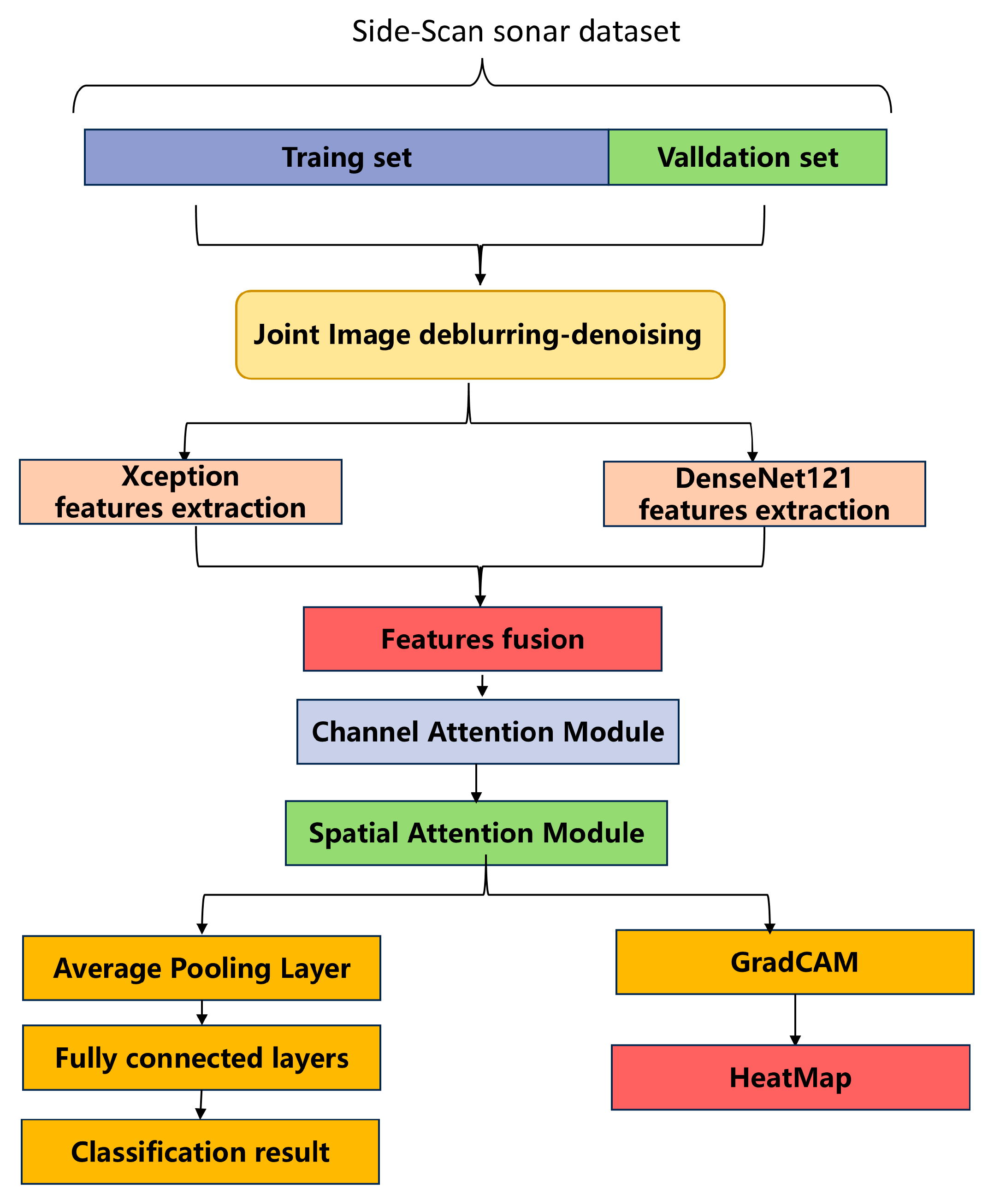
In recent years, deep learning has been increasingly applied to underwater sonar image classification due to its powerful feature extraction capabilities and high efficiency and accuracy. Williams and Fakiris [53] were among the first to introduce convolutional neural networks (CNNs) and combine them with image fusion algorithms for sonar image classification. To further enhance classification performance, Peng et al. [54] proposed a CBL-sinGAN method for side-scan sonar image data augmentation. The CBL module integrates the CBAM (Convolutional Block Attention Module) attention mechanism with the L1 loss function, effectively expanding the dataset of side-scan sonar images. The attention mechanism has been extensively utilized in the domains of image classification. Notably, the Bidirectional Attention and Graph Attention mechanisms warrant particular consideration. Tang et al. [55] introduced bidirectional attention blocks that capture fine-grained information via a novel bidirectional multimodal dynamic routing mechanism. Wang et al. [56] developed the Adaptive Graph Attention (AGA) module to enhance local information and further exploit the interactions between different feature channels. DAI et al. [57] designed a novel GAN that replaces batch normalization (BN) with layer normalization (LN) and uses PReLU activation functions instead of LeakyReLU, enabling more effective image generation and dataset enhancement. SHI et al. [58] combined feature-dense connections and squeeze-and-excitation (SE) modules to propose ShuffleNet-DSE, a deep learning-based classification model that improves classification accuracy. GE et al. [59] integrated RDSNet (Range Doppler heatmap Sequence Detect Network) with ShuffleNetV2 to construct the Shuffle-RDSNet model, which enhances the model’s ability to extract useful features during the feature extraction process. LI et al. [7] proposed a texture feature removal network that narrows the domain gap by discarding domain-specific features. Xu et al. [60] developed an improved CNN model to increase the utilization of sonar image features and reduce misclassification rates for similar categories. Yang et al. [61] introduced MoCo self-supervised learning and used the Swin Transformer with global feature extraction capabilities as a classifier for seabed substrate images, improving the convergence speed and class accuracy.

Although the aforementioned methods have enhanced the classification accuracy of sonar images, they predominantly rely on a single network architecture for feature extraction, focusing primarily on specific features. Consequently, these approaches do not adequately address the multi-scale and multi-level feature extraction requirements essential for side-scan sonar imagery. Additionally, existing methods typically address either low-resolution or high-noise issues but not both comprehensively. This can lead to problems such as noise reduction degrading image quality or super-resolution generating artifacts. Moreover, the limited and imbalanced nature of sonar image datasets continues to restrict the improvement of classification accuracy due to the large amount of data required for training deep learning models.

3. Methods

To further mitigate the adverse effects of poor image quality, weak texture features, blurred edges, insufficient data volume, and sample imbalance on the performance of side-scan sonar image classification, and to enhance the model’s feature representation capability and adaptability to complex underwater environments, this paper proposes a side-scan sonar image classification model based on joint image deblurring–denoising and a pre-trained feature fusion attention network.

As illustrated in Figure 1, this model primarily comprises three key components: the joint image deblurring–denoising method, the feature fusion attention network based on transfer learning, and the technology of Explainable AI (XAI) Grad-CAM.

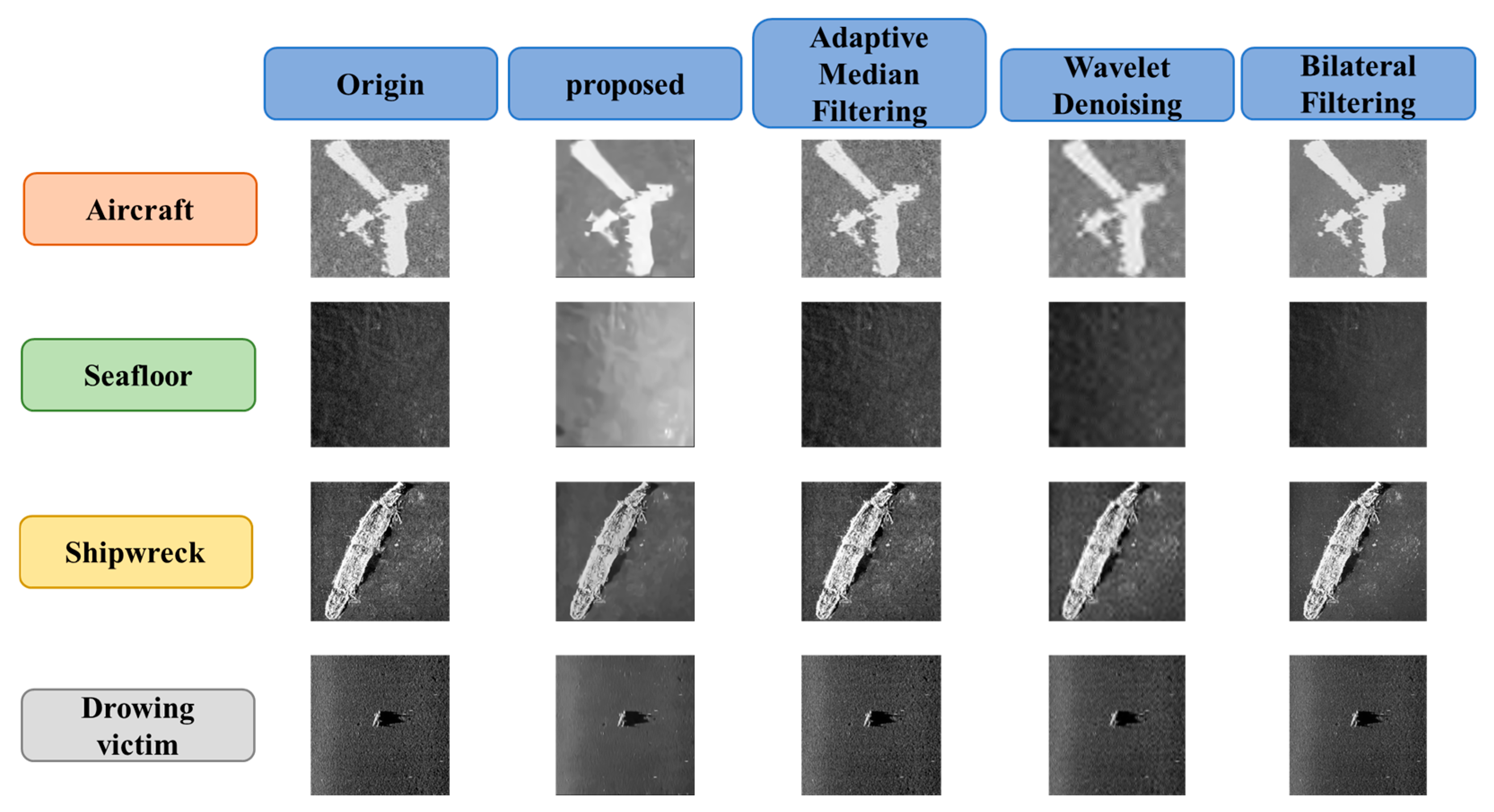
3.1. Joint Image Deblurring–Denoising Method

The joint image deblurring–denoising method restores the edge and texture features of images through 3D transform domain filtering combined with upsampling and downsampling techniques. As illustrated in Figure 2, the process consists of three sequential stages: (1) transform domain hard threshold filtering, (2) RRDB (Residual in Residual Dense Block) upsampling followed by Lanczos downsampling, and (3) transform domain collaborative Wiener filtering. The first stage of transform domain hard threshold filtering initially reduces noise. The second stage, involving RRDB upsampling and Lanczos downsampling reconstruction, effectively restores the texture features of the image. Finally, the third stage further refines the image by eliminating residual noise and addressing potential artifacts introduced during the upsampling process through collaborative Wiener filtering with the pre-upsampling image.

In the remainder of this section, the process of the two transform domain filtering is firstly introduced. Subsequently, the processes of upsampling and downsampling are presented.

For the input image, prior to performing transform domain filtering, block matching and grouping must be conducted. Specifically, the original image is divided into multiple reference blocks of a fixed size. For each reference block, similar blocks within its neighborhood are identified by searching for blocks with an Euclidean distance below a predefined threshold. For a reference block $Y_{x_R}$ of size $N_1^{ht}$ × $N_1^{ht}$ and a similarly sized block $Y_x$ within the neighborhood, the Euclidean distance is calculated using Equation (1):

$$d^{ideal}\left(Y_{x_R},Y_x\right)={\displaystyle \frac{{∥Y_{x_R}-Y_x∥}_2^2}{{\left(N_1^{\mathrm{h}\mathrm{t}}\right)}^2}}.$$

(1)

Subsequently, each group of the divided blocks is transformed into the 3D domain. After filtering in the 3D domain, the data are returned to the original domain via 3D inverse transformation. The joint image deblurring–denoising method involves two transform domain filtering operations. The first one is hard threshold filtering, and the second is collaborative Wiener filtering. Hard threshold filtering uses the original image as its input. Collaborative Wiener filtering, on the other hand, takes both the output from the hard threshold filtering and the output from the resampling module as its inputs. All of the filtering methods can be described by Formula (2). In Formula (2), ${\mathcal{T}}_{3\mathrm{D}}^{\mathrm{h}\mathrm{t}}$ denotes 3D transformation, $\mathsf{{\rm Y}}$ represents filtering, ${\mathcal{T}}_{3\mathrm{D}}^{\mathrm{h}\mathrm{t}-1}$ denotes 3D inverse transformation, $Z_{S_{x_R}^{ht}}$ represents the three-dimensional groups formed after block matching, and ${\widehat{Y}}_{S_{x_R}^{ht}}^{ht}$ represents the processed results of these three-dimensional groups.

$${\widehat{Y}}_{S_{x_R}^{\mathrm{h}\mathrm{t}}}^{\mathrm{h}\mathrm{t}}={\mathcal{T}}_{3\mathrm{D}}^{\mathrm{h}\mathrm{t}-1}\left(\mathsf{{\rm Y}}\left({\mathcal{T}}_{3\mathrm{D}}^{\mathrm{h}\mathrm{t}}\left({\mathrm{Z}}_{S_{x_R}^{\mathrm{h}\mathrm{t}}}\right)\right)\right)$$

(2)

The estimated blocks obtained from the aforementioned process have some overlap. The final image is obtained by aggregating the block estimates using a weighted average approach, as shown in Equation (3). Here, $w_{x_R}^{ht}$ represents the weights, and ${\chi }_{x_m}\left(x\right)$ takes a value of 0 or 1 to indicate whether pixel x belongs to block x_m.

$$\widehat{y}\left(x\right)={\displaystyle \frac{\sum _{x_R\in X}\sum _{x_m\in S_{x_R}^{\mathrm{h}\mathrm{t}}}{w}_{x_R}^{\mathrm{h}\mathrm{t}}{\widehat{Y}}_{x_m}^{\mathrm{h}\mathrm{t},x_R}\left(x\right)}{\sum _{x_R\in X}\sum _{x_m\in S_{x_R}^{\mathrm{h}\mathrm{t}}}{w}_{x_R}^{\mathrm{h}\mathrm{t}}{\chi }_{x_m}\left(x\right)}},\forall x\in X$$

(3)

Between the two stages of transform domain filtering and aggregation, an adversarial training module based on RRDB (Residual in Residual Dense Block) and a U-net discriminator are introduced for upsampling–downsampling reconstruction to restore detailed image features.

The RRDB module is a residual network structure with dense connections. Within an RRDB module, multiple convolutional layers are densely connected and external residual connections are also present. The final output of the RRDB module is the sum of the original input and the result after a series of convolution operations within the module. This residual connection method facilitates easier training of deep networks by allowing gradients to propagate rapidly through the residual connections, ensuring effective training of shallow layers and mitigating the problem of gradient vanishing or rapid decay. Consequently, the densely connected convolutional layers within the RRDB module can effectively extract image features, thereby achieving high-quality image upsampling.

Given the scarcity of target samples in sonar images, the RRDB-based upsampling module is trained using publicly available datasets sourced from the literature [44]. During the training process, original images undergo multiple transformations including blurring, downsampling, adding noise, and JPEG compression to generate low-resolution blurred images. These processed images are then fed into the forward generator network.

After obtaining the output image from the generator network, these generated images are paired with the original image and presented to the U-NET discriminator for evaluation. If the U-NET discriminator struggles to differentiate between the real original image and the generated image, it indicates that a well-trained generator network has been achieved. The entire training process involves iteratively updating the parameters of the generator network using a large number of image inputs. During this process, spectral normalization is employed to stabilize the training. Upon the completion of training, an RRDB network capable of performing upsampling can be obtained.

The downsampling process of the image is based on Lanczos resampling, which is an interpolation method utilizing the sinc function (cardinal sine function). Specifically, this algorithm employs a finite-length sinc function kernel to compute the value of each new pixel. For image downsampling, it calculates weights within a local region of the original image according to the sinc function kernel, then performs a weighted summation of the original image’s pixels to obtain the pixel values in the new image. The influence of each input sample on the interpolation is defined by the resampling kernel L(x), known as the Lanczos kernel. This kernel is a normalized sinc function, and its definition is as Equation (4).

$$L(x)=\left\{\begin{array}{cc}1& \mathrm{i}\mathrm{f}x=0\\ {\displaystyle \frac{a\mathrm{s}\mathrm{i}\mathrm{n}\left(\pi x\right)\mathrm{s}\mathrm{i}\mathrm{n}(\pi x/a)}{{\pi }^2{x}^2}}& \mathrm{i}\mathrm{f}-a\le x<a\mathrm{a}\mathrm{n}\mathrm{d}x\ne 0\\ 0& \mathrm{o}\mathrm{t}\mathrm{h}\mathrm{e}\mathrm{r}\mathrm{w}\mathrm{i}\mathrm{s}\mathrm{e}\end{array}\right.$$

(4)

The pixel grayscale value S(x, y) at coordinate point (x, y) after downsampling is the weighted average of the pixel values within its local neighborhood. For downsampling, when a = 2, the formula can be described by Equation (5):

$$S(x,y)=\sum _{i=\lfloor x\rfloor -a+1}^{\lfloor x\rfloor +a}\sum _{j=\lfloor y\rfloor -a+1}^{\lfloor y\rfloor +a}{s}_{ij}L(x-i)L(y-j).$$

(5)

Compared with simpler downsampling methods such as average pooling, the Lanczos algorithm considers the spatial correlation of pixels in the original image. It employs a sinc function kernel for weighted summation, using more sophisticated weighting schemes to compute the pixel values. This approach better preserves image details and edge information, thereby enhancing the quality of the downsampled image.

3.2. Feature Fusion Attention Network Based on Transfer Learning

This section first introduces the basic principles of transfer learning. It then briefly presents the structures of the feature extraction neural networks Xception and DenseNet, followed by a detailed elaboration on the feature fusion process based on spatial and channel attention mechanisms.

3.2.1. Transfer Learning Method

Transfer learning is a machine learning strategy that leverages knowledge acquired from one or more source tasks to improve performance on a different but related target task.

The following presents the mathematical expression of transfer learning. Given a domain D = {X, P(X)}, X is the feature space and P(X) is its probability distribution. Similarly, a task T = {Y, P(Y|X)} can be obtained, where Y is the label space and P(Y|X) is the conditional probability distribution of the label space under the condition of the feature space. For the source domain Ds, its corresponding task Ts can be obtained. For the target domain Dt, its corresponding task Tt can be obtained. The process of transfer learning is to solve the problems in the target domain Dt and the target task Tt under the condition that Ds ≠ Ts and Dt ≠ Tt by learning the relevant knowledge of the source domain Ds and the source task Ts.

Traditional machine learning methods typically depend on extensive labeled datasets. However, for tasks such as side-scan sonar image classification, the high cost of data annotation limits the availability of large-scale labeled datasets. Training neural networks with limited samples can result in issues like overfitting or model instability. The application of transfer learning can effectively mitigate these challenges.

The methods for implementing transfer learning include fine-tuning, freezing layers, training specific parts of the network, etc. For small sample classification problems like those encountered in sonar image analysis, using complex neural networks with full training can result in overfitting due to the high number of parameters. This paper employs DenseNet and Xception networks, with their end pooling layers and fully connected layers removed, for transfer learning. For DenseNet and Xception networks, pre-training is initially conducted on the ImageNet dataset. Upon the completion of pre-training, the global pooling layer and fully connected layer at the end of these networks are removed, and the remaining portions are integrated into the proposed model as feature extractors. During the subsequent training phase, the weights of the feature extraction components in these networks are frozen, while the newly added layers are trained in the standard manner. Through this approach, effective transfer learning is successfully implemented. Xception excels in multi-scale feature extraction, while DenseNet mitigates overfitting through feature reuse. By combining the complementary features extracted by these two networks at different levels, the model’s feature representation ability and adaptability to complex underwater environments are significantly enhanced.

3.2.2. Introduction of DenseNet and Xception

The core components of the DenseNet architecture are the denseblock and transition modules. In the denseblock module, a dense connection strategy is employed, where each layer’s output is concatenated with the inputs of all subsequent layers through channel-wise concatenation. Dense blocks are interconnected via transition layers, which comprise convolutional layers and pooling layers and can diminish the dimensions of feature maps.

Table 1. The detailed structure of DenseNet used in this paper.

Layers	Output Size	DenseNet-121
Convolution	112 × 112	7 × 7 conv, stride 2
Pooling	56 × 56	3 × 3 max pool, stride 2
Dense Block(1)	56 × 56	$\left[\begin{array}{c}1\times 1\mathrm{c}\mathrm{o}\mathrm{n}\mathrm{v}\\ 3\times 3\mathrm{c}\mathrm{o}\mathrm{n}\mathrm{v}\end{array}\right]$ × 6
Transition Layer(1)	56 × 56	$1\times 1\mathrm{c}\mathrm{o}\mathrm{n}\mathrm{v}$
	28 × 28	2 × 2 average pool, stride 2
Dense Block(2)	28 × 28	$\left[\begin{array}{c}1\times 1\mathrm{c}\mathrm{o}\mathrm{n}\mathrm{v}\\ 3\times 3\mathrm{c}\mathrm{o}\mathrm{n}\mathrm{v}\end{array}\right]$ × 12
Transition Layer(2)	28 × 28	$1\times 1\mathrm{c}\mathrm{o}\mathrm{n}\mathrm{v}$
	14 × 14	2 × 2 average pool, stride 2
Dense Block(3)	14 × 14	$\left[\begin{array}{c}1\times 1\mathrm{c}\mathrm{o}\mathrm{n}\mathrm{v}\\ 3\times 3\mathrm{c}\mathrm{o}\mathrm{n}\mathrm{v}\end{array}\right]$ × 24
Transition Layer(3)	14 × 14	$1\times 1\mathrm{c}\mathrm{o}\mathrm{n}\mathrm{v}$
	7 × 7	2 × 2 average pool, stride 2
Dense Block(4)	7 × 7	$\left[\begin{array}{c}1\times 1\mathrm{c}\mathrm{o}\mathrm{n}\mathrm{v}\\ 3\times 3\mathrm{c}\mathrm{o}\mathrm{n}\mathrm{v}\end{array}\right]$ × 16

details the specific architecture of the network used in this paper. As a feature extractor, this network eliminates the pooling layers and fully connected layers.

Traditional convolutional networks are limited by the unidirectional nature of inter-layer feature transmission, which often results in the loss of shallow detail information at deeper layers, particularly in blurry images. DenseNet addresses this issue through dense cross-layer connections, enabling each layer to receive feature maps from all preceding layers. This facilitates feature reuse and alleviates the vanishing gradient problem via multi-path gradient propagation, thereby empowering the network to (1) extract robust features from noisy data by leveraging complementary multi-level features to suppress local noise and (2) enhance edge reconstruction in low-frequency blurry regions through the synergistic optimization of shallow details and deep semantics. Additionally, DenseNet integrates features via concatenation rather than addition, reducing parameter redundancy while preserving richer feature information. For low SNR sonar images, this design prevents the smoothing of high-frequency details during layer-wise transmission, making it especially effective for target classification.

Depthwise separable convolution (DSC) decomposes the traditional convolution operation into two distinct steps: depthwise convolution and pointwise convolution [62]. Depthwise convolution applies independent convolution operations to each channel of the input image, generating a set of intermediate feature maps. Pointwise convolution then combines these feature maps using 1 × 1 convolution kernels to integrate channel information. In contrast to traditional convolution, where a single convolution kernel operates across all input channels simultaneously, DSC first processes each channel independently with depthwise convolution and subsequently merges the results through pointwise convolution. This approach significantly reduces the number of parameters and decreases inter-layer coupling.

The Xception network is a neural network architecture that leverages depthwise separable convolutions. It first applies spatial convolutions independently to each input channel and then combines the channel information through pointwise convolutions. This design effectively decouples channel-wise and spatial correlations, achieving a high level of separation between these two aspects. By doing so, the Xception architecture significantly reduces the number of model parameters while enhancing computational efficiency. In terms of performance, Xception has demonstrated superior results on benchmark datasets. Specifically, on the ImageNet dataset, Xception outperforms traditional convolutional neural networks by improving accuracy and reducing computational costs.

3.2.3. Feature Fusion Process Based on Spatial and Channel Attention Mechanisms

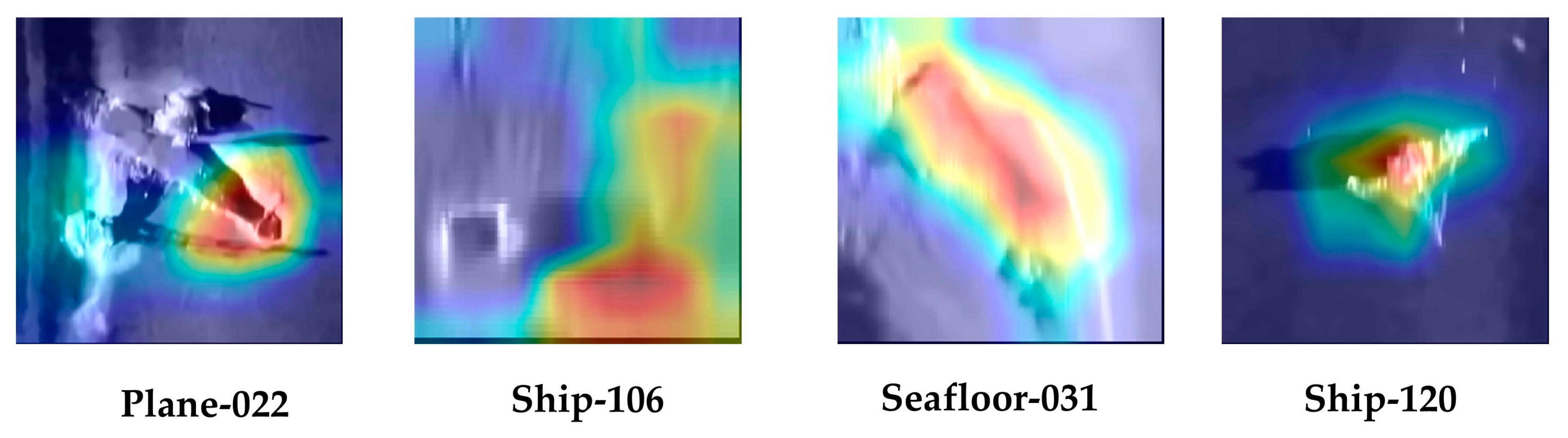
After feature extraction using the densely connected network and the depthwise separable convolution network, the extracted features are concatenated. Subsequently, these concatenated features undergo further fusion through a multi-attention mechanism, which consists of a channel attention mechanism followed by a spatial attention mechanism. The channel attention mechanism adaptively highlights channels that are more significant for classification, while the spatial attention mechanism emphasizes specific spatial regions of the feature map. After applying these two attention mechanisms sequentially, a refined feature map is generated. Subsequently, average pooling is performed on this final feature map, followed by passing it through a fully connected layer to obtain the final classification result.

As for the channel attention mechanism, for each channel of the input feature layer F, global max pooling and global average pooling are performed to obtain two vectors of length equal to the number of channels. These vectors are then passed through fully connected layers to produce two vectors of the same length. The sum of these vectors is passed through an activation function (e.g., sigmoid) to generate the weights for the channel attention mechanism. After obtaining these weights, they are multiplied element-wise with the original input feature layer to implement the channel attention mechanism. During backpropagation, the weights of the channel attention mechanism are optimized to minimize the loss function, enabling the network to focus on the most significant channels for classification.

For the spatial attention mechanism, the maximum and average values across all channels at each spatial location of the input feature layer are computed to obtain a two-channel feature map. This feature map is then processed by a convolutional layer which reduces the number of channels to one. The output is passed through an activation function to obtain the spatial attention weights. These weights are multiplied element-wise with the original input feature layer to implement the spatial attention mechanism. During backpropagation, the parameters of the convolutional kernel are optimized to enable the neural network to focus on the most relevant spatial regions.

After applying the channel attention mechanism and the spatial attention mechanism, the refined feature maps are subsequently processed through pooling and fully connected layers to generate the final classification results.

3.3. Grad CAM

Grad-CAM (Gradient-weighted Class Activation Mapping) is a gradient-based technique designed to visualize the critical image regions that a convolutional neural network (CNN) focuses on during prediction. By utilizing the gradient information of the target class score with respect to the feature maps from the final convolutional layer, Grad-CAM generates a heatmap that intuitively highlights the areas of the input image to which the model assigns higher importance in its decision-making process. Specifically, let A^k represent the k-th feature map of the last convolutional layer and y_c denote the pre-softmax score for the target class c. Grad-CAM first computes the gradient of y_c with respect to A^k and subsequently applies global average pooling (GAP) to these gradients to derive the weight ${\alpha }_k^c$ for each feature map channel k. The calculation formula of ${\alpha }_k^c$ is shown in Equation (6), where Z denotes the product of the width and height of the feature map and $A_{ij}^k$ represents the activation value of the k-th feature map at position (i, j).

$${\alpha }_k^c={\displaystyle \frac{1}{Z}}\sum _i\sum _j{\displaystyle \frac{\partial y^c}{\partial A_{ij}^k}}$$

(6)

Next, the weights ${\alpha }_k^c$ are applied to their corresponding feature maps A^k through a weighted summation to obtain the initial Class Activation Map (CAM), as presented in Equation (7). The ReLU function is subsequently employed to eliminate regions with negative contributions to the target class prediction, thereby emphasizing areas that positively influence the classification outcome.

$$L_{\mathrm{G}\mathrm{r}\mathrm{a}\mathrm{d}-\mathrm{C}\mathrm{A}\mathrm{M}}^c=\mathrm{R}\mathrm{e}\mathrm{L}\mathrm{U}\left(\sum _k{\alpha }_k^c{A}^k\right)$$

(7)

Through the aforementioned steps, the complete process of Grad-CAM (Gradient-weighted Class Activation Mapping) is realized. Subsequently, the calculated weights are fused with the corresponding feature maps via a weighted combination to generate a heatmap. This heatmap is then superimposed onto the original image, thereby visualizing the model’s decision-making process. This procedure visually highlights the critical regions that the model focuses on, providing a robust foundation for enhancing the model’s interpretability.

4. Results and Discussions

4.1. Data Description and Experimental Environment

The data used for evaluation in this study primarily originate from the “Seabed Objects—KLSG Dataset” created by He et al. [63]. Given the absence of drowning victim images in this dataset, a limited number of drowning victim images were selected from the SCTD dataset developed by Zhang et al. [64] to supplement the study. The final dataset is categorized into four categories, i.e., drowning victim, aircraft, shipwreck, and seafloor. This dataset exhibits class imbalance, with a higher proportion of images for shipwrecks and seabed objects compared to those for aircraft and drowning victims. Some representative images are shown in Figure 3. The dataset was split into training and validation sets in a 7:3 ratio for experimentation.

Table 2. The number of images per category in the dataset.

Categories	Drowning Victim	Aircraft	Seafloor	Shipwreck
Numbers	17	66	487	578

details the number of images per category in the dataset.

It is noteworthy that our experiments were conducted exclusively using the publicly available datasets KLSG and SCTD. These datasets consist entirely of side-scan sonar images collected during real underwater detection missions, featuring authentic noise patterns and motion artifacts. This ensures the proposed method’s robust applicability to practical field operations.

As is shown in

Table 3. The hardware and software environment of the experiment.

Component	Description
Processor	12th Gen Intel® Core™ i5—12400F (Intel Corporation, Santa Clara, CA, USA)
Clock Speed	2.5 GHz
RAM	16 GB
Software Environment	Python version: 3.11.7 | packaged by Anaconda, Inc. (Austin, TX, USA) | (main, 15 December 2023, 18:05:47) [MSC v.1916 64 bit (AMD64)] TensorFlow version: 2.12.0 NumPy version: 1.23.5

, the experiments involved in this paper were conducted in the following software and hardware environments.

4.2. Model Performance Metrics

In statistics and machine learning, several key metrics are commonly used to evaluate classification performance. These include:

• True Positive (TP): Samples correctly identified as positive.
• True Negative (TN): Samples correctly identified as negative.
• False Positive (FP): Samples incorrectly identified as positive (actual negatives).
• False Negative (FN): Samples incorrectly identified as negative (actual positives).

Based on these fundamental metrics, additional evaluation metrics can be derived, including Average Precision (AP), Average Recall (AR), the F1 score, Average Specificity (AS), and Overall Accuracy (OA).

• Precision measures the accuracy of the model’s positive predictions, defined as the proportion of true positives among all predicted positives.
• Recall measures the proportion of actual positives that were correctly identified by the model.
• The F1 score is the harmonic mean of precision and recall, providing a balanced measure of both.
• Specificity measures the proportion of actual negatives that were correctly identified as negative.
• Overall Accuracy (OA) measures the proportion of all samples that were correctly classified.

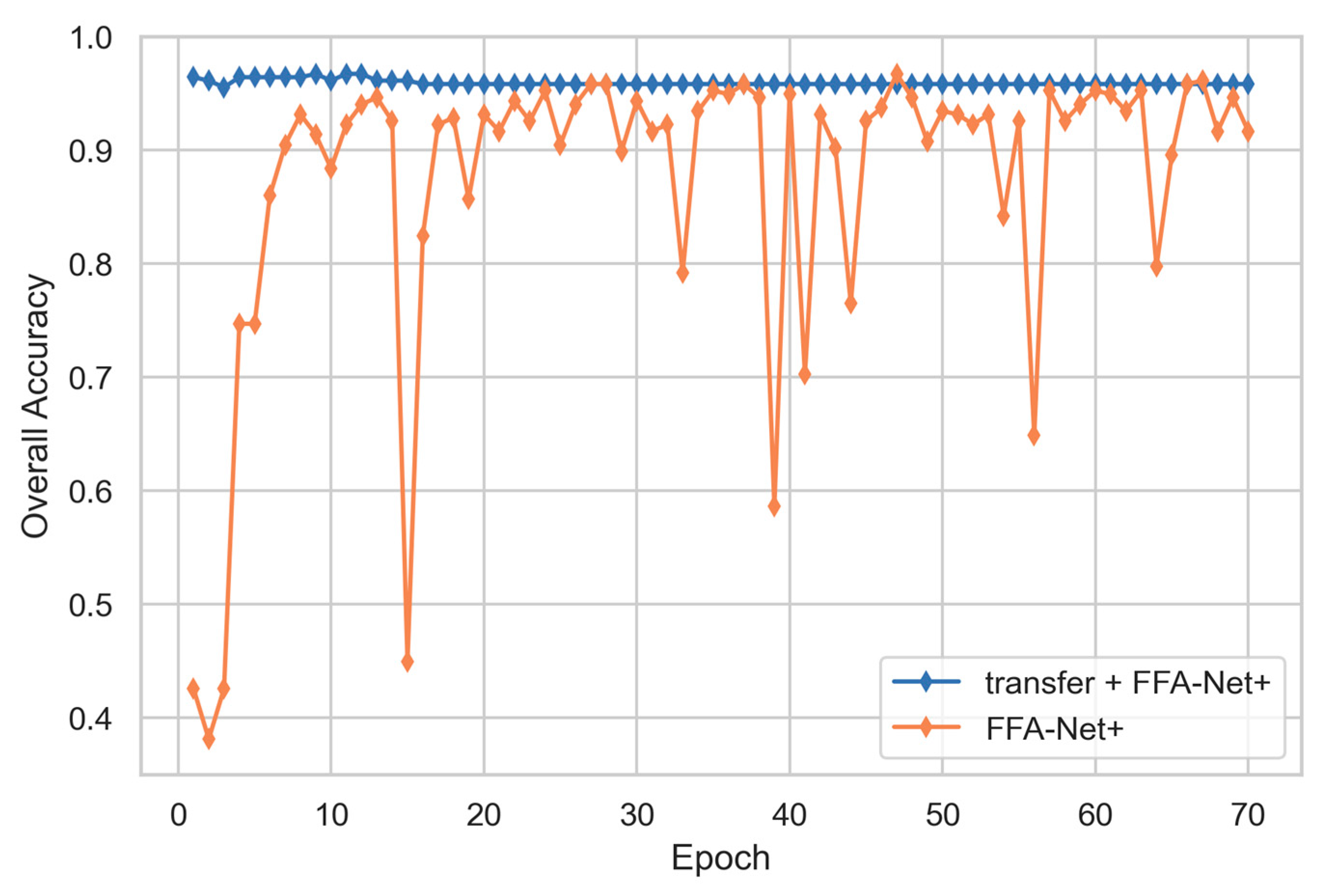
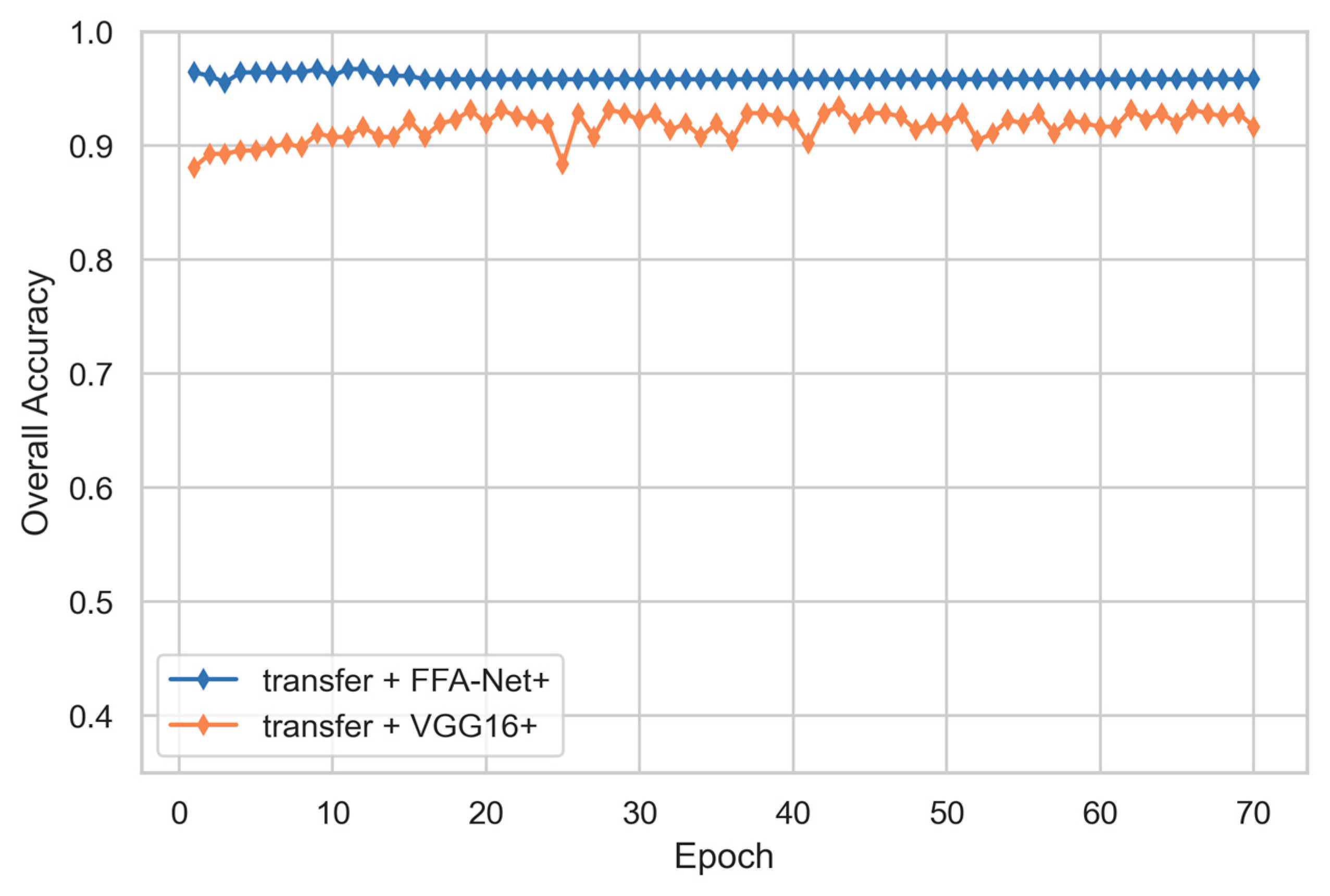
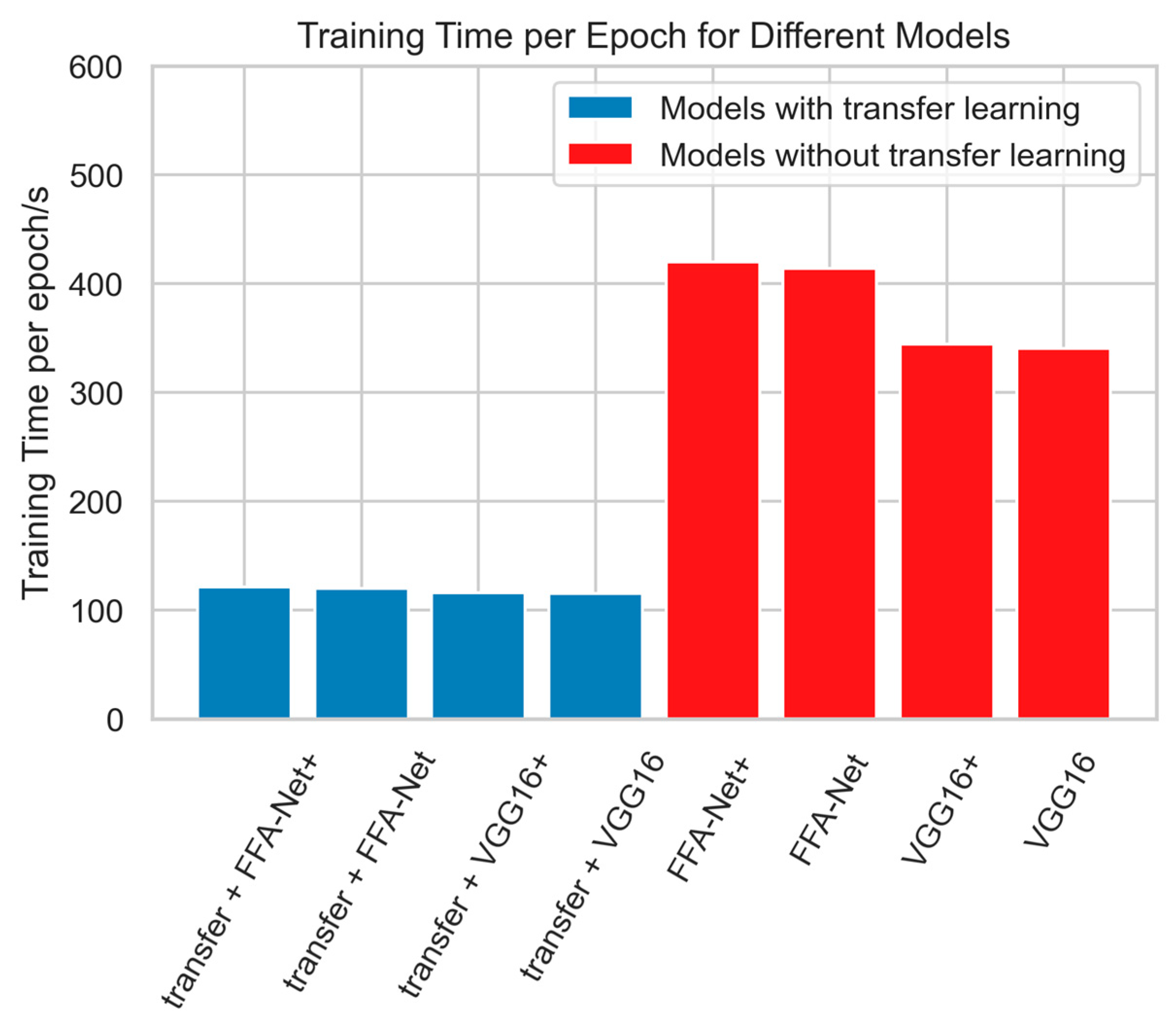
The calculation formulas for each metric are as follows, where N denotes the total number of samples and t denotes the total number of image categories.

$$AP={\displaystyle \frac{TP}{TP+FP}}$$

(8)

$$AR={\displaystyle \frac{TP}{TP+FN}}$$

(9)

$$F_1={\displaystyle \frac{2\times AP\times AR}{AP+AR}}$$

(10)

$$Specificity={\displaystyle \frac{TN}{FP+TN}}$$

(11)

$$OA={\displaystyle \frac{\sum _{i=1}^t{N}_{ii}}{N}}$$

(12)

4.3. Ablation Study

To investigate the contributions of the main modules in the proposed model to classification performance, a total of eight experiments were conducted. These experiments examined the effects of using joint image deblurring–denoising, applying transfer learning, and incorporating the feature fusion attention network (FFA-Net). The results are summarized in

Table 4. Comparison of the average results of different models.

	Model	Transfer Learning	Deblurring– Denoising	OA	AP	AR	F1	AS	Training Time (s/epoch)	Validation Time (ms/per image)
1	FFA-Net	×	×	87.56%	87.56%	88.16%	88.60%	92.47%	414	160
2	FFA-Net	×	√	89.13%	89.12%	89.91%	89.51%	93.37%	420	152
3	FFA-Net	√	×	95.21%	95.21%	95.25%	95.23%	96.71%	120	159
4	FFA-Net	√	√	96.80%	96.80%	96.87%	96.83%	98.07%	121	154
5	VGG16	×	×	84.24%	84.24%	85.79%	84.96%	87.78%	340	143
6	VGG16	×	√	88.02%	88.02%	88.90%	88.44%	94.42%	344	143
7	VGG16	√	×	89.42%	89.41%	89.22%	89.31%	92.15%	115	148
8	VGG16	√	√	91.86%	91.86%	92.09%	91.98%	93.78%	116	141

. To minimize the randomness of the experimental outcomes, each experiment was repeated five times, and the average classification results were recorded. The performance metrics used for evaluation included AP, AR, F1 score, OA, and AS, with the results visualized as box plots in Figure 4.

In this context, “transfer” indicates the application of transfer learning, “FFA-Net” denotes the feature fusion attention network based on dual-path feature extraction using Xception and DenseNet combined with a dual attention mechanism, and the “+” sign signifies the use of the joint image deblurring and denoising method.

The experimental results demonstrate that the introduction of transfer learning significantly enhances model performance. Specifically, the accuracy of the third group of experiments increased by 7.65% compared to the first group, and the accuracy of the fourth group of experiments increased by 7.56% compared to the second group. In the VGG16 network, the accuracy of the seventh group of experiments increased by 5.18% compared to the fifth group, and the accuracy of the eighth group of experiments increased by 3.84% compared to the sixth group. This improvement can be attributed to the fact that large-scale pre-training on the ImageNet dataset generates an efficient feature extractor capable of effectively capturing general image features. Therefore, in small sample tasks, fine-tuning only the pooling and fully connected layers can achieve high classification accuracy. In contrast, deep neural networks without pre-training, due to their large number of parameters and limited training samples, often fail to adequately train network weights, leading to insufficient feature extraction capabilities and a tendency towards overfitting. Additionally, when the sample size is very small, these networks may not converge. The experimental data also indicate that the VGG16 network without transfer learning exhibits significant fluctuations in accuracy and poor model stability. Furthermore, the incorporation of transfer learning has notably reduced the model’s training time. Regarding different network architectures, the FFA-net model proposed in this paper achieves a significant improvement in classification accuracy compared to VGG16, with only a marginal increase in training cost (a few additional seconds per epoch).

The introduction of the joint image deblurring–denoising method further enhances classification performance. The experimental data show that the accuracy of the second group of experiments increased by 1.47% compared to the first group, and the accuracy of the fourth group of experiments increased by 1.48% compared to the third group. In the VGG network, the accuracy of the sixth group of experiments increased by 3.78% compared to the fifth group, and the accuracy of the eighth group of experiments increased by 2.46% compared to the seventh group. This improvement is mainly due to the method’s effectiveness in addressing the high noise and low quality of side-scan sonar images. Specifically, through transform domain filtering, combined with upsampling and downsampling resampling techniques, the edge and texture features of the images are successfully restored, reducing the negative impact of noise and blurring on classification performance. Initially, the first transform domain filtering eliminates image noise, followed by the restoration of image texture features via RRDB upsampling and Lanczos downsampling methods. Finally, the second transform domain filtering removes image noise and artifacts generated during the upsampling process, thereby obtaining high-quality side-scan sonar images.

The introduction of feature fusion and multi-attention mechanisms significantly improves model performance. The experimental results show that the accuracy of the first group of experiments increased by 3.32% compared to the fifth group, the accuracy of the second group of experiments increased by 1.11% compared to the sixth group, the accuracy of the third group of experiments increased by 5.79% compared to the seventh group, and the accuracy of the fourth group of experiments increased by 5.83% compared to the eighth group. This improvement is primarily attributed to the effective integration of the multi-scale feature extraction capabilities of the Xception network with the high accuracy and feature reuse advantages of the densely connected convolutional network through feature fusion and multi-attention mechanisms. By adaptively adjusting the weights of feature layers and image regions that significantly contribute to classification results, the classification effect is further optimized. This fusion mechanism not only improves the efficiency of feature extraction but also effectively alleviates the overfitting problem, thereby achieving a comprehensive enhancement in classification performance.

To assess the statistical significance of the proposed method, this paper conducted a two-tailed paired T-test on the accuracy rates of the proposed method and seven other comparison methods. The test results are summarized in

Table 5. The two-tailed paired T-test on the accuracy rates of the proposed method and seven other comparison methods.

Model	VGG16	VGG16+	Transfer +VGG16	Transfer+ VGG16+	FFA-Net	FFA-Net+	Transfer+ FFA-Net
P	1.8 × 10−3	3.65 × 10−4	5.02 × 10−7	5.02 × 10−8	2.61 × 10−5	4.29 × 10−7	2.29 × 10−5

. All classifiers have p-values significantly lower than 0.05 (p < 0.05). At a significance level of 0.05, we rejected the null hypothesis that “there is no significant difference between the two groups of experiments”, indicating that the proposed method exhibits statistically significant differences in accuracy compared to the methods after the ablation of each module. This result further validates the effectiveness and robustness of the proposed method.

It is worth noting that although the VGG16 network without transfer learning has a lower accuracy rate, its p-value is relatively higher (i.e., the probability that “there is no significant difference between the two groups of experiments” is greater). This phenomenon can be attributed to the larger variance in its accuracy rate, indicating significant fluctuations in model performance. This result further confirms that the model without transfer learning exhibits instability during training, which may lead to poor generalization ability on small sample datasets. The introduction of transfer learning not only significantly improves the accuracy of the model but also reduces the variance in model performance, thereby enhancing the stability and reliability of the model.

To further verify the superiority of the proposed method in small sample classification tasks, Figure 5 illustrates the change curve of validation set accuracy before and after pre-training the neural network. The experimental results show that without transfer learning, the accuracy curve converges more slowly and the final achieved accuracy is relatively low. In contrast, with the introduction of transfer learning, the accuracy curve exhibits a rapid convergence trend, leading to significantly improved final accuracy and more stable network performance.

In addition, Figure 6 presents the curves of the overall accuracy (OA) varying with the number of epochs for the proposed method and the method using VGG16 instead of FFA-Net as the feature extraction network. Both methods demonstrate high stability in classification accuracy after introducing transfer learning. However, the proposed method significantly outperforms the VGG16 network in terms of accuracy.

Furthermore, Figure 7 compares the training time per epoch before and after the introduction of transfer learning. The experimental results indicate that transfer learning significantly accelerates the convergence speed of the network.

As can be seen from Figure 8, Figure 9 and Figure 10, as well as in Table 4, which summarizes the classification accuracy, the pre-trained CNN not only completes the classification task quickly and stably but also significantly improves the classification accuracy.

4.4. Comparative Experiment

To further validate the effectiveness of the multi-attention mechanism and dual-path feature fusion in the hybrid convolutional neural network (CNN), we conducted multiple comparative experiments. Specifically, we replaced the FFA-Net in our proposed method (transfer + FFA-Net) with other single networks. The experimental results are summarized in

Table 6. Classification performance of different models.

Model	OA	AP	AR	F1	AS
FFA-Net	96.80%	96.80%	96.87%	96.83%	98.07%
VGG16	91.86%	91.86%	91.68%	91.77%	94.27%
MobileNetV2	93.31%	93.31%	93.28%	93.30%	95.54%
DenseNet121	94.48%	94.47%	94.65%	94.56%	96.24%
InceptionV3	94.77%	94.77%	94.82%	94.80%	96.41%

.

To further validate the superiority of combining the Xception and DenseNet121 networks, we conducted additional experiments comparing the performance of various network combinations. The results are summarized in

Table 7. Classification performance of models using different dual-path feature extractors.

Model	OA	AP	AR	F1	AS
Xception+DenseNet121	96.80%	96.80%	96.87%	96.83%	98.07%
InceptionV3+MobileNetV2	94.77%	94.83%	94.80%	94.77%	96.10%
Xception+InceptionV3	95.35%	95.35%	95.40%	95.37%	96.64%
Xception+MobileNetV2	95.64%	95.64%	95.67%	95.65%	97.20%
DenseNet121+MobileNetV2	93.90%	93.89%	93.96%	93.93%	95.73%

. Furthermore, as illustrated in

Table 8. Comparison of our model with the confusion matrix of other models using different dual-path feature extractors.

Model	True Class	Predicted Class
		Shipwreck	Aircraft	Seafloor	Drowning Victim
Xception+DenseNet121	Shipwreck	143	2	1	0
	Aircraft	1	19	0	0
	Seafloor	6	0	167	0
	Drowning Victim	0	0	0	5
InceptionV3+MobileNetV2	Shipwreck	142	1	3	0
	Aircraft	9	11	0	0
	Seafloor	4	0	169	0
	Drowning Victim	1	0	0	4
Xception+InceptionV3	Shipwreck	140	2	4	0
	Aircraft	2	18	0	0
	Seafloor	8	0	165	0
	Drowning Victim	0	0	0	5
Xception+MobileNetV2	Shipwreck	142	2	2	0
	Aircraft	5	15	0	0
	Seafloor	6	0	167	0
	Drowning Victim	0	0	0	5
DenseNet121+MobileNetV2	Shipwreck	142	2	2	0
	Aircraft	9	11	0	0
	Seafloor	8	0	165	0
	Drowning Victim	0	0	0	5

, the evaluation results of our proposed model are compared against those of other models using their respective confusion matrices.

The experimental results demonstrate that the combination of Xception and DenseNet121 exhibits high classification stability across all categories and achieves the highest overall classification accuracy. When either Xception or DenseNet121 is individually replaced by other networks, the classification accuracy of the hybrid model decreases. For instance, InceptionV3 + MobileNetV2 and DenseNet121 + MobileNetV2 perform poorly in classifying aircraft, with a significant number of aircraft being misclassified as shipwrecks. These comparative experiments further confirm the complementary advantages of the Xception and DenseNet121 networks in side-scan sonar image classification.

To further substantiate the efficacy of the proposed attention mechanism in this study, a comparative analysis was conducted against other existing attention methods, including the spatial attention method (SAM) and the channel attention method (CAM). The results are shown in

Table 9. Classification performance of models using different attention methods.

Model	OA	AP	AR	F1	AS
proposed	96.80%	96.80%	96.87%	96.83%	98.07%
CAM	95.64%	95.64%	95.77%	95.70%	97.10%
SAM	96.22%	96.22%	96.31%	96.27%	97.53%

. The FFA-Net employs a spatial–channel joint attention mechanism, which adaptively identifies and prioritizes the channels and image regions that contribute most significantly to image classification. In comparison with standalone spatial or channel attention mechanisms, the proposed approach demonstrates superior performance across multiple evaluation metrics, including OA, AP, AR, F1, and AS. These results confirm the superiority of the spatial–channel joint attention mechanism over its single-component counterparts and provide robust validation for the effectiveness of the proposed method.

To further substantiate the superiority of the joint image deblurring–denoising method proposed in this paper, comparative experiments were conducted using different denoising techniques. Figure 8 shows the comparison of the processing results of the proposed method with those of other methods. The results indicate that the joint image deblurring–denoising method outperforms adaptive median filtering, wavelet denoising, and bilateral filtering in multiple aspects. Specifically, compared with adaptive median filtering, the proposed method achieves a more balanced presentation of image details, effectively mitigating the over-sharpening of artifacts and enhancing the naturalness and realism of image features. In contrast to wavelet denoising, the proposed method produces images with a more uniform gray-level distribution, successfully reducing graininess caused by residual noise and thereby improving visual quality. Furthermore, when compared with bilateral filtering, the proposed method not only preserves edge information more effectively but also demonstrates superior capability in suppressing background noise.

Taking specific examples, as shown in Figure 8, the “aircraft” image processed by the proposed method exhibits a clearer and more distinguishable fuselage outline. For the “shipwreck” image, the texture details of the hull are better preserved and presented. Additionally, the proposed method significantly reduces noise interference in images such as “seafloor”, resulting in a smoother background, while enhancing the distinction between targets and backgrounds in images like “drowning victim”. Overall, the images processed by the proposed method are characterized by enhanced clarity and readability, providing a more robust foundation for subsequent in-depth analysis and processing.

Moreover,

Table 10. Comparison of the classification performance of the joint image denoising–deblurring method with those of other methods.

Model	OA	AP	AR	F1	AS
Proposed	96.80%	96.80%	96.87%	96.83%	98.07%
Adaptive mean filtering	93.60%	93.60%	93.77%	93.69%	95.63%
Bilateral filtering	92.15%	92.15%	92.62%	92.39%	94.54%
Wavelet filtering	95.64%	95.64%	95.62%	95.63%	97.05%

illustrates the comparative outcomes of classification performance. The classification performance evaluations confirm that the application of the proposed joint image deblurring–denoising method leads to a significant improvement in image classification accuracy. In comparison, simple filtering algorithms such as adaptive mean filtering and bilateral filtering yield unsatisfactory results, while wavelet filtering, although producing acceptable outcomes, still lags behind the proposed method in terms of overall performance.

Furthermore, this paper conducts a comparative analysis with state-of-the-art methods. ConvNeXt, proposed by the Meta (formerly Facebook) AI team, is a convolutional neural network architecture that integrates the strengths of traditional CNNs with modern network design principles to modernize the ResNet series of networks. Swin Transformer, developed by Microsoft Research Asia, is a visual model architecture based on the Transformer framework that reduces computational complexity via a hierarchical window-based attention mechanism and effectively captures multi-scale image features. The proposed method in this paper achieves superior performance compared to these advanced methods in terms of accuracy, recall, F1 score, and specificity, thereby further validating the effectiveness of the proposed approach. The results are shown in

Table 11. Classification performance of the proposed model and other state-of-the-art methods.

Model	OA	AP	AR	F1	AS
FFA-Net	96.80%	96.80%	96.87%	96.83%	98.07%
CovnNext [65]	95.93%	96.11%	95.93%	95.99%	97.82%
Swin Transformer [66]	95.06%	95.24%	95.06%	95.13%	97.37%

.

Extensive comparative experiments and multi-dimensional performance analyses indicate that the method employed in this paper significantly outperforms other approaches in terms of effectiveness. From the perspective of algorithmic complexity, our method is comparable to existing alternatives.

Currently, while the method demonstrates excellent performance outcomes, there remains room for improvement in image processing speed. To enhance the convenience and real-time applicability of this method in actual use cases, it is imperative to optimize algorithmic workflows, adopt more efficient data structures, or leverage advanced hardware acceleration techniques to increase the processing speed of each image. This will better meet the demands of practical applications.

4.5. Case Study and Grad-CAM Result

To further validate the effectiveness of our proposed model, we conducted a detailed analysis using specific case studies.

Table 12. Comparison of our model with the confusion matrix of the model without joint image deblurring–denoising, without transfer learning, or using VGG16 as an alternative to FFA-Net.

Model	True Class	Predicted Class
		Shipwreck	Aircraft	Seafloor	Drowning Victim
Proposed (pre-trained FFA-Net with joint image deblurring–denoising)	Shipwreck	143	2	1	0
	Aircraft	1	19	0	0
	Seafloor	6	0	167	0
	Drowning Victim	0	0	0	5
Pre-trained FFA-Net (without joint image deblurring–denoising)	Shipwreck	141	2	3	0
	Aircraft	7	13	0	0
	Seafloor	5	0	168	0
	Drowning Victim	1	0	0	4
FFA-Net with joint image deblurring–denoising (without transfer learning)	Shipwreck	145	1	0	0
	Aircraft	16	2	2	0
	Seafloor	14	0	159	0
	Drowning Victim	3	0	0	2
Pre-trained VGG16 with joint image deblurring–denoising	Shipwreck	139	3	4	0
	Aircraft	11	9	0	0
	Seafloor	8	0	165	0
	Drowning Victim	1	0	0	4

presents the confusion matrices for four different configurations: the proposed method (pre-trained FFA-Net with joint image deblurring–denoising), the method without joint image deblurring–denoising, the method without transfer learning, and the method using VGG16 as the alternative to FFA-Net. The experimental results demonstrate that introducing joint image deblurring–denoising along with transfer learning significantly improves the classification performance. Additionally, the feature fusion attention network (FFA-Net) proposed in this paper outperforms VGG16 in terms of classification accuracy.

The introduction of the joint image deblurring–denoising method significantly improved the classification accuracy for aircraft. Among a total of 20 aircraft samples, the number of correct classifications increased from 13 to 19. As shown in Figure 9, before applying the joint image deblurring–denoising method, six aircraft images were misclassified.

After implementing the joint image deblurring–denoising method, these images were correctly classified. As illustrated in Figure 10, the joint image deblurring–denoising method effectively reduced image noise, restored texture features, and consequently enhanced the classification accuracy.

Furthermore, as is shown in Table 9, after the introduction of transfer learning, the classification accuracy for aircraft and drowning victims has significantly improved. This indicates that transfer learning is essential for addressing imbalanced datasets. Without transfer learning, the model tends to overfit to the abundant data for shipwrecks and seafloors while underfitting to the scarce samples of aircraft and drowning victims. Consequently, it learns a large number of features for common categories but fewer features for minority categories, leading to the misclassification of rare samples (such as aircraft and drowning victims) as more common ones (like shipwrecks or seafloors). After introducing transfer learning, the model can better capture the features of minority categories, thereby significantly improving classification accuracy. This improvement is attributed to the excellent feature extractor obtained through pre-training on ImageNet, which effectively mitigates the challenges posed by imbalanced datasets and enhances the model’s generalization ability.

To gain an intuitive understanding of the model’s feature extraction capabilities, Figure 11 illustrates partial feature maps extracted by the first convolutional layer after ablating different modules. Specifically, it compares the proposed method in this paper with three ablated versions: without joint image deblurring–denoising, without transfer learning, and using VGG16 as the alternative to FFA-Net.

The experimental results show that the method proposed in this paper can significantly enhance the saliency of the target contour during the feature extraction process, and the extracted features have higher clarity and discriminability. The features extracted by the method without the joint image deblurring–denoising have noise and blurring phenomena. The feature maps extracted using the VGG16-based model exhibit insufficient contrast, making it challenging to distinguish between the foreground and background. The performance of the FFA-Net method without using transfer learning is close to that after using transfer learning, but using transfer learning can still slightly improve the quality of the extracted feature maps (the first feature map is clearer, and after swapping the positions of the second and eighth feature maps, the clarity of the second to eighth feature maps is similar). In summary, the method in this paper better retains the detailed information of the target in the feature space, reduces the influence of noise and low resolution, and thus provides more discriminative feature representations for subsequent classification tasks. This further verifies the effectiveness of the joint image deblurring–denoising method, FFA-Net, and transfer learning strategy in improving the feature extraction ability of the model.

Grad-CAM (Gradient-weighted Class Activation Mapping), as an efficient interpretability tool, can explain and verify the decision-making process of deep learning models in a visual way. Through in-depth analysis of these visualization results, we can better understand the basis of the model’s decision-making, thereby providing important support for model performance optimization and the improvement of classification accuracy.

As shown in Figure 12, the heatmap generated by Grad-CAM is superimposed onto the original sonar image. The heatmap is generated by analyzing the gradient of the model’s prediction with respect to the pixel values of the input image. Through different colors, the heatmap clearly distinguishes the regions that play a key role in the model’s classification decision. Specifically, warm tones such as red and yellow indicate that these parts have a significant contribution to the model’s classification decision; while cold tones such as blue and green mean that their influence on the classification decision is relatively low. This superimposition method can visually correspond the key regions that the model focuses on with the content of the original image, thereby enabling the rapid localization of the model’s key focus areas and enhancing the model’s interpretability.

The different colors in the figure are obtained through normalization processing for each individual image, representing relative weights. Grad-CAM heat maps have demonstrated strong interpretability across various image recognition tasks. In seafloor images, it is typically challenging to precisely locate large target objects, resulting in relatively uniform weights across the entire region. For shipwreck images, the model can accurately delineate the contours due to the larger number of training samples. For images related to aircraft and drowning victims, where the training set contains fewer samples, the model can still determine the target locations.

Figure 13 shows the heatmap generated by Grad-CAM superimposed onto incorrectly classified sonar images of different categories. The image numbered plane-022 was misclassified as a ship. Its contour is distinctive, primarily composed of numerous regular straight lines. Visually, the constructed shape bears a high resemblance to common ship shapes, with a prominent end to the contour. The image numbered ship-106 was incorrectly labeled as seabed substrate due to poor image quality. The ship in the image is too blurry to recognize clearly. Seafloor-031 was misclassified as a ship because the protruding parts of the seabed resemble ship-like structures. The image numbered ship-120 was erroneously classified as an aircraft. Analysis revealed that the ship’s unusual posture, specifically its overturned state, caused its overall contour to resemble that of an aircraft, leading to the model’s misjudgment.

In the aforementioned images, for those misclassified as aircraft or ships, the heatmap effectively highlights the regions to which the model pays significant attention. Conversely, for images misclassified as seabed substrates, the heatmap exhibits a relatively uniform weight distribution. Furthermore, these misclassified images inherently possess characteristics that can mislead human judgment. Overall, the model exhibits strong interpretability.

Grad-CAM effectively enhances the interpretability and transparency of sonar image classification in underwater rescue scenarios, ensuring that classification decisions are grounded in key underwater target features. This capability is crucial for building trust in AI applications within the underwater rescue domain. Understanding the rationale behind model predictions provides a scientific basis for rescue decisions, thereby significantly improving the efficiency of rescue operations. Additionally, high-weight regions highlighted in the heat maps can alert rescue personnel to potential targets, increasing the likelihood of successful rescue efforts.

5. Conclusions

To address the challenges posed by poor image quality, weak texture features, and blurred edges during the feature extraction of side-scan sonar images, we propose a joint image deblurring–denoising method. This method restores edge and texture details through transform domain filtering, combined with upsampling and downsampling techniques. Additionally, a transfer learning training strategy that selectively freezes certain weights is applied to the dual-path feature extractor based on Xception and DenseNet to prevent overfitting on small sample sizes. To further enhance classification accuracy, we introduce the Feature Fusion Attention Network (FFA-Net). FFA-Net leverages the efficiency and multi-scale feature extraction capabilities of depthwise separable convolutions, along with the accuracy and feature reuse benefits of densely connected networks. FFA-Net incorporates dual attention mechanisms to adaptively focus on specific channels and feature map regions, effectively extracting key features from side-scan sonar images and enhancing the importance of critical feature channels and regions.

The proposed model has shown significant improvement in performance metrics, with OA, AP, AR, F1 score, and AS reaching 96.80%, 96.80%, 96.87%, 96.83%, and 98.07%, respectively. The two-tailed paired t-test indicates that the proposed method exhibits statistically significant differences in accuracy compared to the methods with each module ablated.

In the comparative experiments, the FFA-Net achieves significantly higher classification accuracy than single networks (e.g., DenseNet) and combinations where the feature extraction network was replaced by MobileNet, Inception, etc. This result demonstrates the complementary strengths of Xception and DenseNet in feature extraction and the significant advantage of using the attention mechanisms to achieve adaptive feature fusion.

Furthermore, the comparisons of extracted feature maps and the interpretability analysis using Grad-CAM confirm the strong interpretability of the proposed method.

In future research, we can further improve model performance by integrating more advanced feature extraction networks such as GoogleNet and deeper ResNet architectures and by expanding the dataset through the design of an effective image generation network for side-scan sonar images, thereby enhancing classification accuracy.

References

1. Greene, A.; Rahman, A.F.; Kline, R.; Rahman, M.S. Side scan sonar: A cost-efficient alternative method for measuring seagrass cover in shallow environments. Estuar. Coast. Shelf Sci. 2018, 207, 250–258. [Google Scholar] [CrossRef]
2. Boretti, A. Unmanned surface vehicles for naval warfare and maritime security. J. Def. Model. Simul. 2024, 15485129241283056. [Google Scholar] [CrossRef]
3. Silarski, M.; Nowakowski, M. Performance of the SABAT neutron-based explosives detector integrated with an unmanned ground vehicle: A simulation study. Sensors 2022, 22, 9996. [Google Scholar] [CrossRef]
4. Munteanu, D.; Moina, D.; Zamfir, C.G.; Petrea, Ș.M.; Cristea, D.S.; Munteanu, N. Sea mine detection framework using YOLO, SSD and EfficientDet deep learning models. Sensors 2022, 22, 9536. [Google Scholar] [CrossRef]
5. Niemikoski, H.; Söderström, M.; Kiljunen, H.; Östin, A.; Vanninen, P. Identification of degradation products of sea-dumped chemical warfare agent-related phenylarsenic chemicals in marine sediment. Anal. Chem. 2020, 92, 4891–4899. [Google Scholar] [CrossRef] [PubMed]
6. Tang, Y.; Wang, L.; Jin, S.; Zhao, J.; Huang, C.; Yu, Y. AUV-based side-scan sonar real-time method for underwater-target detection. J. Mar. Sci. Eng. 2023, 11, 690. [Google Scholar] [CrossRef]
7. Li, C.; Ye, X.; Xi, J.; Jia, Y. A texture feature removal network for sonar image classification and detection. Remote Sens. 2023, 15, 616. [Google Scholar] [CrossRef]
8. McMahon, J.; Plaku, E. Autonomous data collection with timed communication constraints for unmanned underwater vehicles. IEEE Robot. Autom. Lett. 2021, 6, 1832–1839. [Google Scholar] [CrossRef]
9. Ling, H.; Zhu, T.; He, W.; Zhang, Z.; Luo, H. Cooperative search method for multiple AUVs based on target clustering and path optimization. Nat. Comput. 2021, 20, 3–10. [Google Scholar]
10. Cao, X.; Ren, L.; Sun, C. Research on obstacle detection and avoidance of autonomous underwater vehicle based on forward-looking sonar. IEEE Trans. Neural Networks Learn. Syst. 2022, 34, 9198–9208. [Google Scholar]
11. Fan, X.; Lu, L.; Shi, P.; Zhang, X. A novel sonar target detection and classification algorithm. Multimed. Tools. Appl. 2022, 81, 10091–10106. [Google Scholar]
12. Chen, Z.; Wang, Y.; Tian, W.; Liu, J.; Zhou, Y.; Shen, J. Underwater sonar image segmentation combining pixel-level and region-level information. Comput. Electr. Eng. 2022, 100, 107853. [Google Scholar]
13. Karimanzira, D.; Renkewitz, H.; Shea, D.; Albiez, J. Object detection in sonar images. Electronics 2020, 9, 1180. [Google Scholar] [CrossRef]
14. Wang, Y.; Wang, H.; Li, Q.; Xiao, Y.; Ban, X. Passive sonar target tracking based on deep learning. J. Mar. Sci. Eng. 2022, 10, 181. [Google Scholar] [CrossRef]
15. Zou, S.; Lin, J.; Wang, X.; Li, G.; Wang, Z.; Xie, X. An object enhancement method for forward-looking sonar images based on multi-frame fusion. In Proceedings of the 2021 IEEE International Symposium on Circuits and Systems (ISCAS), Daegu, Republic of Korea, 22–28 May 2021; pp. 1–5. [Google Scholar]
16. Li, S.; Zhao, J.; Zhang, H.; Bi, Z.; Qu, S. A non-local low-rank algorithm for sub-bottom profile sonar image denoising. Remote Sens. 2020, 12, 2336. [Google Scholar] [CrossRef]
17. Yang, C.; Li, Y.; Jiang, L.; Huang, J. Foreground enhancement network for object detection in sonar images. Mach. Vis. Appl. 2023, 34, 56. [Google Scholar]
18. Najibzadeh, M.; Mahmoodzadeh, A.; Khishe, M. Active sonar image classification using deep convolutional neural network evolved by robust comprehensive grey wolf optimizer. Neural Process Lett. 2023, 55, 8689–8712. [Google Scholar]
19. Shi, P.; Sun, H.; Fan, X.; He, Q.; Zhou, X.; Lu, L. An effective automatic object detection algorithm for continuous sonar image sequences. Multimed. Tools. Appl. 2024, 83, 10233–10246. [Google Scholar]
20. Goodman, J.W. Speckle Phenomena in Optics: Theory and Applications; Roberts and Company Publishers: Greenwood Village, CO, USA, 2007. [Google Scholar]
21. Cheng, Z.; Huo, G.; Li, H. A multi-domain collaborative transfer learning method with multi-scale repeated attention mechanism for underwater side-scan sonar image classification. Remote Sens. 2022, 14, 355. [Google Scholar] [CrossRef]
22. Liu, T.; Yan, S.; Wang, G. Remove and recover: Two stage convolutional autoencoder based sonar image enhancement algorithm. Multimed. Tools. Appl. 2024, 83, 55963–55979. [Google Scholar]
23. Rao, J.; Peng, Y.; Chen, J.; Tian, X. Various Degradation: Dual Cross-Refinement Transformer For Blind Sonar Image Super-Resolution. IEEE Trans. Geosci. Remote Sens. 2024, 62, 1–14. [Google Scholar]
24. Yuan, F.; Xiao, F.; Zhang, K.; Huang, Y.; Cheng, E. Noise reduction for sonar images by statistical analysis and fields of experts. J. Vis. Commun. Image Represent. 2021, 74, 102995. [Google Scholar]
25. Vishwakarma, A. Denoising and inpainting of sonar images using convolutional sparse representation. IEEE Trans. Instrum. Meas. 2023, 72, 1–9. [Google Scholar]
26. Zhou, T.; Si, J.; Wang, L.; Xu, C.; Yu, X. Automatic detection of underwater small targets using forward-looking sonar images. IEEE Trans. Geosci. Remote Sens. 2022, 60, 1–12. [Google Scholar]
27. Klaucke, I. Sidescan Sonar; Springer: Berlin/Heidelberg, Germany, 2018; pp. 13–24. [Google Scholar]
28. Sadjadi, F.A. Studies in adaptive automated underwater sonar mine detection and classification-part 1: Exploitation methods. In Proceedings of the Automatic Target Recognition XXV, Baltimore, MD, USA, 19 June 2015; pp. 157–172. [Google Scholar]
29. Jiao, W.; Zhang, J. Sonar images classification while facing long-tail and few-shot. IEEE Trans. Geosci. Remote Sens. 2022, 60, 1–20. [Google Scholar]
30. Ye, X.; Yang, H.; Li, C.; Jia, Y.; Li, P. A gray scale correction method for side-scan sonar images based on retinex. Remote Sens. 2019, 11, 1281. [Google Scholar] [CrossRef]
31. Ge, Q.; Ruan, F.; Qiao, B.; Zhang, Q.; Zuo, X.; Dang, L. Side-scan sonar image classification based on style transfer and pre-trained convolutional neural networks. Electronics 2021, 10, 1823. [Google Scholar] [CrossRef]
32. Kapetanović, N.; Mišković, N.; Tahirović, A. Saliency and anomaly: Transition of concepts from natural images to side-scan sonar images. IFAC-PapersOnLine 2020, 53, 14558–14563. [Google Scholar]
33. Yu, G.; Sapiro, G. DCT image denoising: A simple and effective image denoising algorithm. Image Process. Line 2011, 1, 292–296. [Google Scholar]
34. Danielyan, A.; Katkovnik, V.; Egiazarian, K. BM3D frames and variational image deblurring. IEEE Trans. Image Process 2011, 21, 1715–1728. [Google Scholar]
35. Zhang, K.; Zuo, W.; Chen, Y.; Meng, D.; Zhang, L. Beyond a gaussian denoiser: Residual learning of deep cnn for image denoising. IEEE Trans. Image Process 2017, 26, 3142–3155. [Google Scholar]
36. Chen, P.; Xu, Z.; Zhao, D.; Guo, X. Despeckling for forward looking sonar image based on ANLResNet. J. Chin. Comput. Syst. 2022, 43, 355–361. [Google Scholar]
37. Tian, C.; Xiao, J.; Zhang, B.; Zuo, W.; Zhang, Y.; Lin, C.-W. A self-supervised network for image denoising and watermark removal. Neural Netw. 2024, 174, 106218. [Google Scholar]
38. Tang, H.; Zhang, W.; Zhu, H.; Zhao, K. Self-supervised real-world image denoising based on multi-scale feature enhancement and attention fusion. IEEE Access 2024, 12, 49720–49734. [Google Scholar]
39. Fan, L.; Cui, J.; Li, H.; Yan, X.; Liu, H.; Zhang, C. Complementary blind-spot network for self-supervised real image denoising. IEEE Trans. Circuits Syst. Video Technol. 2024, 34, 10107–10120. [Google Scholar]
40. Zhou, X.; Yu, C.; Yuan, X.; Luo, C. Deep denoising method for side scan sonar images without high-quality reference data. In Proceedings of the 2022 2nd International Conference on Computer, Control and Robotics (ICCCR), Shanghai, China, 18–20 March 2022; pp. 241–245. [Google Scholar]
41. Lim, B.; Son, S.; Kim, H.; Nah, S.; Mu Lee, K. Enhanced deep residual networks for single image super-resolution. In Proceedings of the IEEE Conference on Computer Vision and Pattern Recognition Workshops, Honolulu, HI, USA, 21–26 July 2017; pp. 136–144. [Google Scholar]
42. Zhang, Y.; Li, K.; Li, K.; Wang, L.; Zhong, B.; Fu, Y. Image super-resolution using very deep residual channel attention networks. In Proceedings of the European Conference on Computer Vision (ECCV), Munich, Germany, 8–14 September 2018; pp. 286–301. [Google Scholar]
43. Wang, X.; Yu, K.; Wu, S.; Gu, J.; Liu, Y.; Dong, C.; Qiao, Y.; Change Loy, C. Esrgan: Enhanced super-resolution generative adversarial networks. In Proceedings of the European Conference on Computer Vision (ECCV) Workshops, Munich, Germany, 8–14 September 2018. [Google Scholar]
44. Wang, X.; Xie, L.; Dong, C.; Shan, Y. Real-esrgan: Training real-world blind super-resolution with pure synthetic data. In Proceedings of the IEEE/CVF International Conference on Computer Vision, Virtually, 11–17 October 2021; pp. 1905–1914. [Google Scholar]
45. Yan, Y.; Liu, C.; Chen, C.; Sun, X.; Jin, L.; Peng, X.; Zhou, X. Fine-grained attention and feature-sharing generative adversarial networks for single image super-resolution. IEEE Trans. Multimed. 2021, 24, 1473–1487. [Google Scholar]
46. Lu, Z.; Zhu, T.; Zhou, H.; Zhang, L.; Jia, C. An image enhancement method for side-scan sonar images based on multi-stage repairing image fusion. Electronics 2023, 12, 3553. [Google Scholar] [CrossRef]
47. Peng, C.; Jin, S.; Bian, G.; Cui, Y. SIGAN: A Multi-Scale Generative Adversarial Network for Underwater Sonar Image Super-Resolution. J. Mar. Sci. Eng. 2024, 12, 1057. [Google Scholar] [CrossRef]
48. Zhu, B.; Wang, X.; Chu, Z.; Yang, Y.; Shi, J. Active learning for recognition of shipwreck target in side-scan sonar image. Remote Sens. 2019, 11, 243. [Google Scholar] [CrossRef]
49. Karine, A.; Lasmar, N.; Baussard, A.; El Hassouni, M. Sonar image segmentation based on statistical modeling of wavelet subbands. In Proceedings of the 2015 IEEE/ACS 12th International Conference of Computer Systems and Applications (AICCSA), Marrakech, Morocco, 17–20 November 2015; pp. 1–5. [Google Scholar]
50. Kumar, N.; Mitra, U.; Narayanan, S.S. Robust object classification in underwater sidescan sonar images by using reliability-aware fusion of shadow features. IEEE J. Ocean. Eng. 2014, 40, 592–606. [Google Scholar]
51. Zhu, M.; Song, Y.; Guo, J.; Feng, C.; Li, G.; Yan, T.; He, B. PCA and kernel-based extreme learning machine for side-scan sonar image classification. In Proceedings of the 2017 IEEE Underwater Technology (UT), Busan, Republic of Korea, 21–24 February 2017; pp. 1–4. [Google Scholar]
52. Liu, X.; Zhu, H.; Song, W.; Wang, J.; Yan, L.; Wang, K. Research on improved VGG-16 model based on transfer learning for acoustic image recognition of underwater search and rescue targets. IEEE J. Sel. Top. Appl. Earth Obs. Remote Sens. 2024, 17, 18112–18128. [Google Scholar]
53. Williams, D.P.; Fakiris, E. Exploiting environmental information for improved underwater target classification in sonar imagery. IEEE Trans. Geosci. Remote Sens. 2014, 52, 6284–6297. [Google Scholar]
54. Peng, C.; Jin, S.; Bian, G.; Cui, Y.; Wang, M. Sample Augmentation Method for Side-Scan Sonar Underwater Target Images Based on CBL-sinGAN. J. Mar. Sci. Eng. 2024, 12, 467. [Google Scholar] [CrossRef]
55. Tang, J.; Liu, D.; Jin, X.; Peng, Y.; Zhao, Q.; Ding, Y.; Kong, W. BAFN: Bi-direction attention based fusion network for multimodal sentiment analysis. IEEE Trans. Circuits Syst. Video Technol. 2022, 33, 1966–1978. [Google Scholar]
56. Wang, H.; Liu, J.; Tan, H.; Lou, J.; Liu, X.; Zhou, W.; Liu, H. Blind image quality assessment via adaptive graph attention. IEEE Trans. Circuits Syst. Video Technol. 2024, 34, 10299–10309. [Google Scholar]
57. Dai, Z.; Liang, H.; Duan, T. Small-sample sonar image classification based on deep learning. J. Mar. Sci. Eng. 2022, 10, 1820. [Google Scholar] [CrossRef]
58. Shi, Y.; Chen, M.; Yao, C.; Li, X.; Shen, L. Seabed Sediment Classification for Sonar Images Based on Deep Learning. Comput. Inform. 2022, 41, 714–738. [Google Scholar]
59. Ge, Q.; Liu, H.; Ma, Y.; Han, D.; Zuo, X.; Dang, L. Shuffle-RDSNet: A method for side-scan sonar image classification with residual dual-path shrinkage network. J. Supercomput. 2024, 80, 19947–19975. [Google Scholar]
60. Xu, Y.; Wang, X.; Wang, K.; Shi, J.; Sun, W. Underwater sonar image classification using generative adversarial network and convolutional neural network. IET Image Process 2020, 14, 2819–2825. [Google Scholar]
61. Yang, Y.; Wang, Y.; Yang, Z.; Yang, J.; Deng, L. Research on the classification of seabed sediments sonar images based on MoCo self-supervised learning. In Proceedings of the Journal of Physics: Conference Series, Changsha, China, 13–15 October 2024; p. 012058. [Google Scholar]
62. Chollet, F. Xception: Deep learning with depthwise separable convolutions. In Proceedings of the IEEE Conference on Computer Vision and Pattern Recognition, Honolulu, HI, USA, 21–26 July 2017; pp. 1251–1258. [Google Scholar]
63. Huo, G.; Wu, Z.; Li, J. Underwater object classification in sidescan sonar images using deep transfer learning and semisynthetic training data. IEEE Access 2020, 8, 47407–47418. [Google Scholar]
64. Zhang, P.; Tang, J.; Zhong, H.; Ning, M.; Liu, D.; Wu, K. Self-trained target detection of radar and sonar images using automatic deep learning. IEEE Trans. Geosci. Remote Sens. 2021, 60, 1–14. [Google Scholar] [CrossRef]
65. Liu, Z.; Lin, Y.; Cao, Y.; Hu, H.; Wei, Y.; Zhang, Z.; Lin, S.; Guo, B. Swin transformer: Hierarchical vision transformer using shifted windows. In Proceedings of the IEEE/CVF International Conference on Computer Vision, Virtually, 11–17 October 2021; pp. 10012–10022. [Google Scholar]
66. Liu, Z.; Mao, H.; Wu, C.-Y.; Feichtenhofer, C.; Darrell, T.; Xie, S. A convnet for the 2020s. In Proceedings of the IEEE/CVF Conference on Computer Vision and Pattern Recognition, New Orleans, LA, USA, 19–24 June 2022; pp. 11976–11986. [Google Scholar]
Figure 1. Overall structure of the proposed model.
Electronics 14 01287 g001
Figure 2. Process of joint image deblurring–denoising.
Electronics 14 01287 g002
Figure 3. Some examples of side-scan sonar images.
Electronics 14 01287 g003
Figure 4. Plots of the classification results. Transfer + denotes transfer learning, and + denotes using “joint image deblurring–denoising”.
Electronics 14 01287 g004
Figure 5. The change curve of the validation set accuracy before and after pre-training the neural network. Transfer + denotes transfer learning, and + denotes using “joint image deblurring–denoising”.
Electronics 14 01287 g005
Figure 6. The change curve of the validation set accuracy of FFA-Net and VGG16. Transfer + denotes transfer learning, and + denotes using “joint image deblurring–denoising”.
Electronics 14 01287 g006
Figure 7. The training time per epoch before and after the introduction of transfer learning.
Electronics 14 01287 g007
Figure 8. Comparison of the processing results of the joint image denoising–deblurring method with those of other methods.
Electronics 14 01287 g008
Figure 9. Aircraft images that are misclassified by the method without the joint image deblurring–denoising method.
Electronics 14 01287 g009
Figure 10. The output of the aircraft images after being processed by the joint image deblurring and denoising method.
Electronics 14 01287 g010
Figure 11. Comparison of the partial feature maps extracted by the first convolutional layer.
Electronics 14 01287 g011
Figure 12. The heatmap generated by Grad-CAM superimposed onto the original sonar image of different categories.
Electronics 14 01287 g012
Figure 13. The heatmap generated by Grad-CAM superimposed onto the incorrectly classified sonar images of different categories.
Electronics 14 01287 g013