Efficient Compression of Red Blood Cell Image Dataset Using Joint Deep Learning-Based Pattern Classification and Data Compression

Abstract

Millions of people across the globe are affected by the life-threatening disease of Malaria. To achieve the remote screening and diagnosis of the disease, the rapid transmission of large-size microscopic images is necessary, thereby demanding efficient data compression techniques. In this paper, we argued that well-classified images might lead to higher overall compression of the images in the datasets. To this end, we investigated the novel approach of joint pattern classification and compression of microscopic red blood cell images. Specifically, we used deep learning models, including a vision transformer and convolutional autoencoders, to classify red blood cell images into normal and Malaria-infected patterns, prior to applying compression on the images classified into different patterns separately. We evaluated the impacts of varying classification accuracy on overall image compression efficiency. The results highlight the importance of the accurate classification of images in improving overall compression performance. We demonstrated that the proposed deep learning-based joint classification/compression method offered superior performance compared with traditional lossy compression approaches such as JPEG and JPEG 2000. Our study provides useful insights into how deep learning-based pattern classification could benefit data compression, which would be advantageous in telemedicine, where large-image-size reduction and high decoded image quality are desired.

1. Introduction

Malaria poses a significant public health challenge globally, especially in Malaria-endemic regions. It is among the primary causes of mortality and illness in numerous developing nations, particularly impacting young children and pregnant women the most [1]. In 2022, it was estimated that Malaria led to 249 million cases and resulted in 608,000 fatalities across the globe [2]. Various techniques exist for diagnosing Malaria, including the gold-standard approach that involves the microscopic analysis of blood smears. However, this method requires trained professionals and involves procedures that consume considerable time and are susceptible to errors [3]. The time duration imposes a significant constraint on the rapid diagnosis of the infection, necessitating the development of more efficient methods for Malaria diagnoses. Consequently, ongoing research focuses on leveraging computer-aided techniques to improve the diagnosis of Malaria infection.

A significant amount of research has been conducted focusing on the application of deep learning in Malaria diagnosis in the recent years [4]. In most of the prior experiments, microscopic images were used [5,6,7,8,9,10]. There are a few studies where whole-slide images were used to develop automated methods for Malaria detection [11,12,13]. One major drawback of using whole-slide images is their higher resolution, which requires extensive computational resources. These high-resolution images require considerable memory and processing power, potentially slowing down analysis and increasing operational costs. Also, this drawback hampers the smooth and rapid transmission of images to specialists situated in different geographically located areas for consultation and screening due to large image sizes. Nonetheless, sufficiently high resolution is essential to determining the exact species and the severity of infection [14]. To address this need, increasingly effective solutions have emerged, especially through deep learning-based compression algorithms. The exponential growth of medical images has directed researchers to focus on memory- and transmission-efficient image compression approaches using deep learning methods [15,16,17]. Several studies have been conducted to analyze the efficiency of compressing medical images by using deep learning methods [18,19,20]. Additionally, deep learning methods have shown excellent performance in the task of image classification. However, in-depth study of the impact of misclassification rates on data compression efficiency when using deep learning remains relatively sparse.

Most of the existing work studies data compression and classification independently. There are a few studies where compression and classification were performed jointly [21,22,23,24,25,26,27,28]. In this section, we survey briefly existing studies on combined data compression and classification. In [22], general-purpose and genomic-specific compressors were utilized to effectively diagnose organisms in metagenomic samples. The study demonstrated the relationship between compression and classification, underscoring the need for a comprehensive approach to improve classification. A deep learning-based method was presented for the compression and classification of whole-slide histopathology images in [24]. This approach uses ROI-based neural networks to extract meaningful features that are important for accurate classification. In [23], a novel approach named Iterative Gaussian–Laplacian Pyramid Network (IGLPN) was developed to classify hyperspectral images. The method uses both Gaussian and Laplacian pyramids to generate a compact representation of images, which is then combined with a deep learning approach to perform classification. The method studied in [25] employs encryption and JPEG compression on the images used for classification using a vision transformer. The paper shows that significant classification performance can be achieved even after applying JPEG compression on encrypted images without compromising accuracy. In [26], the authors proposed a 2C-Net framework that combines image compression and classification via deep neural networks. The main focus of the paper is to find the generalized shared features suitable for serving dual purposes. The study in [27] reveals that the classification accuracy does not entirely depend on the compression rate. In the research study, large language models were used as compressors to support the conclusion. The paper [28] proposes the co-compression via superior gene (CC-SG) technique, which uses a joint pruning–quantization method to optimize convolutional neural networks for image classification. The technique adopts an enhanced evolution algorithm that finds the superior genes that eventually compress the network.

None of the above studies analyzed the trade-offs between the classification rate and compression efficiency. In our prior work [29], we offered a probabilistic analysis of how misclassification rates influence stacked autoencoder-based lossless compression efficiency, especially by using the information-theoretic entropy metric. In contrast, this work focuses on more practical implementations, where we evaluated the effect of misclassification rates on lossy compression that utilizes deep learning approaches. More specifically, we processed methods by integrating classification and compression into a single workflow, potentially enhancing the efficiency of medical diagnosis and reducing transmission overhead. The ability to perform this dual functionality is vital in healthcare sectors, where the quick and precise identification of diseases and optimized data management are necessary. Next, we evaluated how the classification performance affects the efficiency of the data compressor that was trained by using the classified data obtained from the classifiers in the previous step.

Considering the superior pattern classification performance of deep neural networks, it is important to assess the effect of misclassification on image compression. In this paper, we used two different deep learning architectures (a dual-purpose autoencoder model and a hybrid model) for the detection of Malaria infection and compared their performance on two different datasets. Initially, the proposed model performed the classification of the dataset. Next, we fed the classified data derived from each of the classifiers to different compressors. Finally, we measured the compression ratios for each of the joint classification and compression networks. Since the classification accuracy varied for each of the networks, the study provides insights into how the misclassification rate affects overall compression efficiency on the entire datasets.

This paper is structured as follows: Section 2 introduces the background and provides the details of the methods used in this work; Section 3 presents the results of the study; Section 4 discusses the results and provides a comparative analysis of the methods; Section 5 outlines the limitations and suggests directions for further research; the paper is concluded in Section 6.

2. Materials and Methods

2.1. Autoencoders

Autoencoders, also known as AEs, are neural networks specifically created to acquire efficient data representations by using a self-supervised learning method. AEs comprise two main parts, an encoder and a decoder, which collaborate to reconstruct the input data. The encoder transforms the data into a lower-dimensional latent representation via non-linear transformation, whereas the decoder attempts to replicate the actual input from the latent space. Autoencoders reduce the data dimension by keeping only the necessary characteristics for reconstructing the input data. This design enables AEs to effectively extract features and grasp important patterns and structures from data.

2.1.1. Sparse Autoencoders

Sparse autoencoders are neural networks designed for the unsupervised learning of compact representations. Unlike conventional autoencoders, sparse autoencoders focus on particular high-level characteristics in the data while disregarding most other aspects. This is accomplished by applying a sparsity constraint on the hidden units during the training process. The degree of sparsity can be managed by either manually deactivating specific hidden units, adjusting the activation functions, or incorporating a loss term into the cost function. Sparse autoencoders have been applied in numerous areas, including anomaly detection, denoising, and dimensionality reduction.

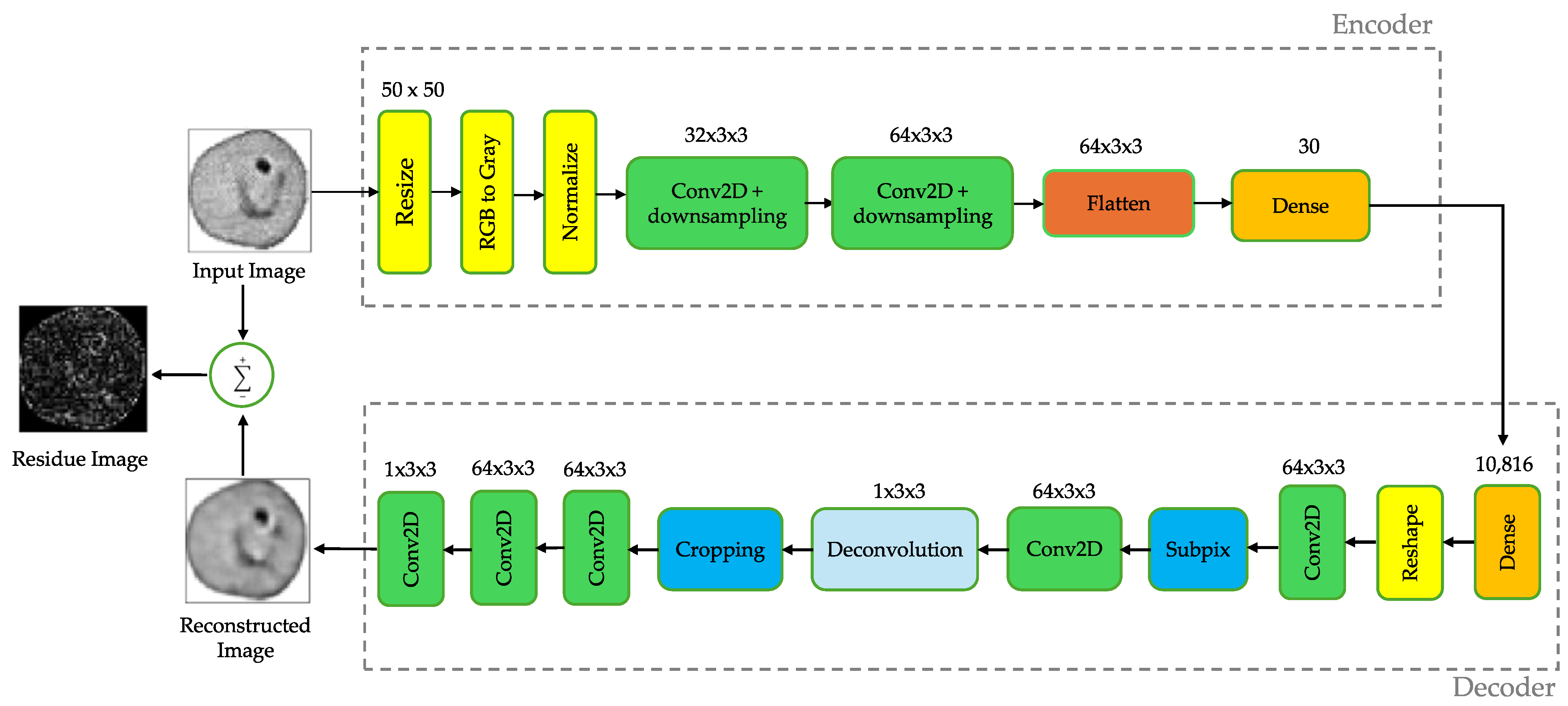
2.1.2. Convolutional Autoencoders

Autoencoders that use convolutional layers, known as convolutional autoencoders (CAEs), are unsupervised learning models that are particularly designed for handling high-dimensional data. The primary goal of the CAEs is to compress the data while learning the essential information, effectively extracting the important features in the process [30]. The main difference between traditional autoencoders and convolutional autoencoders is that CAEs include convolutional layers in their structure. These layers employ learnable kernels or filters to carry out convolutions on the input, gathering features at various levels of hierarchy and scales. CAEs prove to be beneficial, as they are capable of grasping spatial and temporal relationships through filters. By leveraging these capabilities, CAEs can perform different tasks, such as image processing, image compression, and image denoising [31,32].

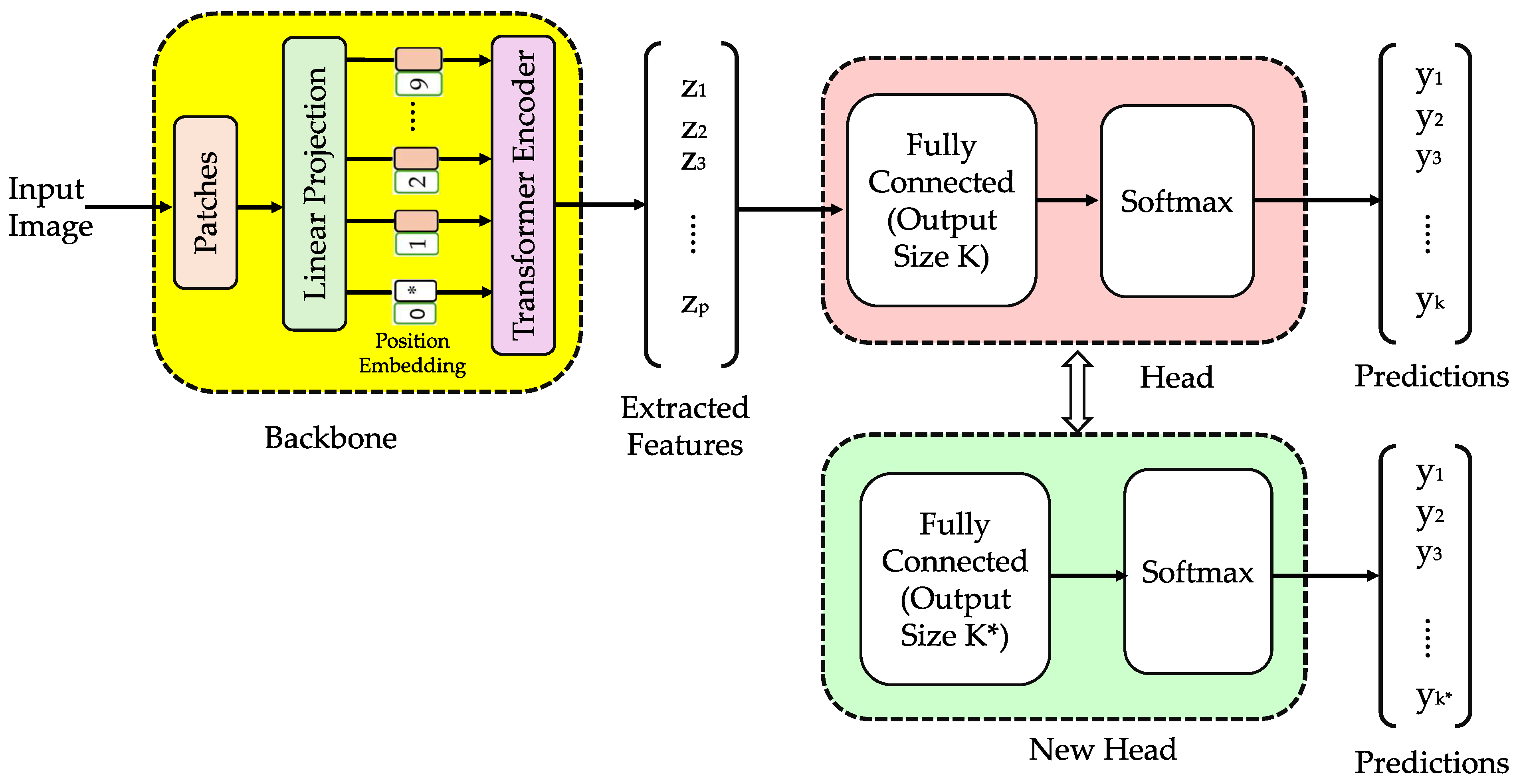
2.2. Vision Transformer

The vision transformer (ViT) is a type of neural network architecture that leverages the self-attention mechanism to derive inherent features [33]. The ViT has become a popular method for natural language processing (NLP) tasks. Unlike traditional convolutional neural networks (CNNs), which employ convolutional layers, fully connected layers, and pooling layers to extract spatial hierarchies in images, the ViT operates by dividing an image into smaller, fixed-size patches. Each patch is then embedded into vectors, and these vectors are fed as input to the transformer blocks, which are made up of several stacked layers of self-attention and feed-forward networks. The transformer operates on the embedded vectors, subsequently mapping them linearly to the required input dimension [34]. The ViT’s capacity to capture long-range dependencies makes it appropriate for a range of vision tasks, including image classification [35] and object detection [36].

2.3. Development of Deep Learning Models for Image Classification

A significant number of deep learning techniques have been developed in the past few decades for the classification of images. Ref. [37] is an excellent review on how deep learning models, particularly deep neural networks and autoencoders, continue to develop and influence various domains, specifically image classification. The review places a lot of emphasis on autoencoders, investigating their potential for feature learning and dimensionality reduction as precursors to image classification. A comprehensive analysis of the field of convolutional neural networks (CNNs) is offered in [38], demonstrating their robust abilities in handling image classification tasks. The survey outlines critical training challenges in CNNs and studies solutions to improve performance. CNNs are the most widely used models for the tasks of image classification due to their noticeable performance [39]. The advances in deep learning approaches have led to the vision transformer (ViT). In [40], the authors demonstrate that the transformer-based architecture allows for greater accuracy than CNNs. In addition, it has been shown that ViTs can be lighter than CNNs, requiring less training time and computational resources. To understand how autoencoders and ViTs perform image classification, we will provide an overview of the technical aspects of these architectures.

2.3.1. Stacked Autoencoders for Image Classification

A stacked autoencoder (SAE) is a type of deep autoencoder in which several encoders are stacked on top of each other, along with multiple decoders stacked similarly. For a model to be classified as “stacked”, it must contain multiple hidden layers to avoid singularity in the hidden layers. Similar to the autoencoders, the SAE employs the activation function. Additionally, the SAE utilizes the backpropagation algorithm and computes the loss function by using Mean Square Error (MSE) [41]. In order to perform classification, a classification layer has to be mounted on top of the last layer of the SAE. Once this deep network is built, it is trained by using the standard supervised approach [42].

2.3.2. Vision Transformer for Image Classification

Vision transformers (ViTs) operate directly on sequences of image patches for the purpose of image classification. The initial stage consists of segmenting the input image into smaller, non-overlapping patches. These patches are then flattened and transformed into a vector that serves as an input token. The idea of patching was influenced by the tokenization method utilized in NLP, which transforms words into embeddings [33]. To obtain these patches ready for the transformer model, a linear projection is used to transform each flattened patch into an embedding of fixed dimension. This conversion allows the model to manage patches with different content while maintaining consistent representation sizes, making processing more straightforward [35]. A significant challenge in utilizing the transformer architecture for images is how to preserve spatial information. Unlike text data, where sequence matters, spatial continuity is vital in images. As a result, positional encodings are incorporated into each patch embedding to uphold the arrangement and spatial organization of the patches. These encodings convey the position of each patch within the original image, enabling the model to understand the spatial relationships between various parts of the image [40]. This capability is essential to effectively interpreting the overall organization and context of images. The patch embeddings, enhanced with positional data, are input into a typical transformer encoder. This encoder is made up of successive layers that include multi-head self-attention and feed-forward neural networks. The self-attention mechanism allows the model to identify which areas of the image should be emphasized when generating predictions [40]. The multi-head attention mechanism is deployed to enhance the performance of the self-attention layers by generating different representation subspace of the input vectors. A unique learnable class embedding is concatenated at the start of the patch sequence before being passed through the encoder [35]. As the data move through the transformer, the output from the encoder is then directed through a feed-forward network (often a Multi-Layer Perceptron, or MLP) to generate the ultimate classification outcome [35].

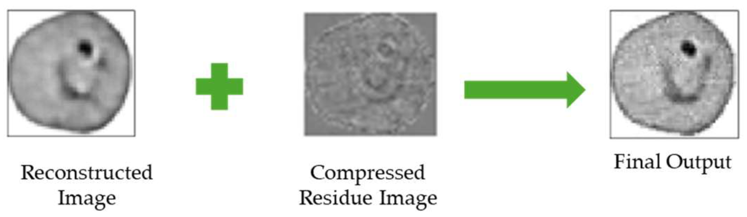
2.4. Lossy Image Compression

There are primarily two categories of lossy image compression methods, classified by their compression techniques: linear and non-linear. JPEG is the most popular imaging format that uses the linear lossy compression algorithm. JPEG encoding starts by dividing the image into blocks of $8\times 8$ pixels. Each block undergoes a Discrete Cosine Transform (DCT), which shifts the spatial information into frequency components, highlighting the distinction between high and low frequencies. These components are then quantized, to reduce the precision of higher-frequency components that are less noticeable to the human eye [43]. Next, a zigzag scan is applied, arranging the coefficients from low to high frequency and clustering similar frequencies together. In order to reduce the file size by eliminating redundancy, the data stream is then compressed by using entropy encoding techniques such as Run-Length Encoding and Huffman coding [44]. Similar to the JPEG standard, the Joint Photographic Experts Group developed JPEG 2000 to serve as an enhanced version of the JPEG format, offering a superior compression ratio that results in higher-quality images. In order to achieve that, JPEG 2000 encoding utilizes the Discrete Wavelet Transform (DWT) to assess the entire image within a cohesive framework, bypassing the block-based method of JPEG. This transformation provides a multi-resolution depiction of the image, allowing for more precise adjustments of image features and textures. After the transformation, the wavelet coefficients undergo quantization to focus on crucial visual content while eliminating the less relevant information. The quantized coefficients are subsequently processed with the Embedded Block Coding with Optimal Truncation (EBCOT) algorithm, which enhances compression by treating different blocks independently [43]. This approach facilitates effective entropy coding and allows for the progressive enhancement of the image during transmission.

Deep learning-based models have become a popular non-linear image compression technique. These models use a complex and non-linear generative technique to learn the compact representation of data [17,45]. A typical deep learning architecture that uses the non-linear compression technique is the autoencoder. Autoencoders consist of two parts: an encoder and a decoder. The encoder part generates the compressed data, while the decoder reproduces the input from the compressed data. Because of their popularity in reducing the dimensionality of the image, autoencoders have gained popularity in image compression [41,46,47]. Our proposed architectures utilize autoencoders for compression while integrating a classifier to enhance compression, using the classified images as images of same class sharing common features that aid the machine learning algorithm to efficiently extract compressed features. In our architectures, we deployed two distinct classifiers: an autoencoder and a vision transformer. Autoencoders’ efficiency in feature extraction and dimensionality reduction is crucial to transforming high-dimensional data into a format that enhances the efficacy of the classification process. On the other hand, the vision transformer shows superior performance in processing complex image data, leveraging its self-attention mechanism that identifies the relevant areas for accurate classification. The data classified with the two classifiers with varying accuracy allow for a comprehensive evaluation of the performance of the compressor. The integration of these classification models in our architectures ensures the standard performance of our compression model.

2.5. Malaria Datasets

2.5.1. UAB_Dataset

The whole-slide images used in this research study were sourced from the PEIR-VM repository established by the medical school of University of Alabama, Birmingham [48,49]. Multiple efficient image processing operations, such as image segmentation and removal of noisy pixels, were applied to generate individual cell images. After image pre-processing, a large number of cell images were randomly selected and examined by the pathologists at University of Alabama, Birmingham, in our prior collaborative efforts. After careful examination by multiple pathologists, the final labeled dataset was created. In this dataset, there are 2565 cell images, among which 1034 belong to the infected class and the remaining 1531 belong to the normal or non-infected class. We then subdivided the entire dataset into test and training image datasets, where 117 images were inserted into the test dataset for both classes and the remaining were used as the training dataset for their respective class.

2.5.2. NIH_Dataset

The cell images within the dataset were collected from thin blood smears photographed at Chittagong Medical College Hospital, Bangladesh [50]. The dataset comprises 27,558 cell images from 193 patients, featuring an equal number of parasitized (infected) and uninfected cells and available on the National Institutes of Health (NIH) website. The annotations in the dataset encompass various characteristics found in blood samples, including dead_parasite, white blood cells, and additional components, like debris or air bubbles. For our research, the dataset was partitioned into training and test subsets. The subset used for testing comprised 1378 images for each class, resulting in a total of 2756 test images. The remainder of the images were allocated to the training set.

2.6. Proposed Lossy Compression Architecture

The compression module consists of two main parts: the convolutional autoencoder (CAE) and the residual block. The CAE seeks to generate images that resemble the input images as closely as possible. The difference between the image generated by the CAE and the original input is calculated as the residue. The residue is then compressed by using a traditional codec and combined with the compact representation obtained from the encoder to produce the final compressed bitstream. Figure 1 illustrates the block diagram of the proposed CAE. The framework of the CAE includes two main components: the encoder and the decoder. The encoder converts the input image into a latent representation, and the decoder recovers the input from the compact representation generated by the encoder.

The encoder portion of the architecture starts with pre-processing steps, which include resizing the image to $50\times 50$ pixels, followed by extracting the red channel only. The uniformity in input image size is a fundamental requirement for batch processing in deep neural networks. Extracting the red channel simplifies the model by reducing computational complexity without affecting the essential information within the images. Each pixel of the processed image is then divided by 255 to normalize the pixel value to a fractional number between 0 and 1. This step is vital, as it improves the speed of testing and allows for faster convergence by standardizing the scale among all input features. The encoder has two convolutional layers, each of which is accompanied by LeakyReLU activations and batch normalization. Batch normalization stabilizes training by effectively minimizing the internal covariate shift [51]. The first convolutional layer has 32 filters, followed by a max-pooling operation with a $2\times 2$ window for downsampling, which reduces the dimension of the feature maps from $50\times 50$ to $25\times 25$. The second layer consists of 64 filters, followed by max-pooling operation with a window size of $2\times 2$, generating feature maps of $12\times 12$ resolution. After convolution and max pooling, the feature maps are flattened and compressed down to a 30-dimensional vector by using a dense layer which is the bottleneck layer of the encoder.

The decoder begins by expanding the 30-point vector from the bottleneck layer into a $\mathrm{10,816}$ tensor through a dense layer. Subsequently, this $1D$ tensor is reshaped into a $3D$ tensor of dimensions $13\times 13\times 64$ that can be processed further via a sequence of convolutional layers; the model progressively enhances the spatial features, recovering details that were abstracted during the encoding phase. After the first convolutional layer with 32 filters, there is a sub-pixel layer that enhances the resolution of the feature maps from $13\times 13$ to $26\times 26$ by rearranging the data points in the tensor, increasing the image resolution while maintaining the depth [52]. A transposed convolutional (deconvolution) layer is added next to the second convolutional layer, which further upscales the map to a $52\times 52$ resolution. The resulting output is then precisely cropped to the desired dimensions of $50\times 50$ pixels, to be consistent with the original input size. Next, three consecutive convolutional layers are applied with the number of filters being 64, 64, and 1 to further refine the image, ensuring that the output image captures or restores details that accurately reflect the original input.

By subtracting the reconstructed image from the original input, we obtain the residue. The residue is then passed through the residue block (Figure 2), where it undergoes JPEG 2000 compression. Finally, the compressed residue is combined with the reconstructed image from the CAE to enhance the quality of the reconstructed image and generate the final result, as shown in Figure 3.

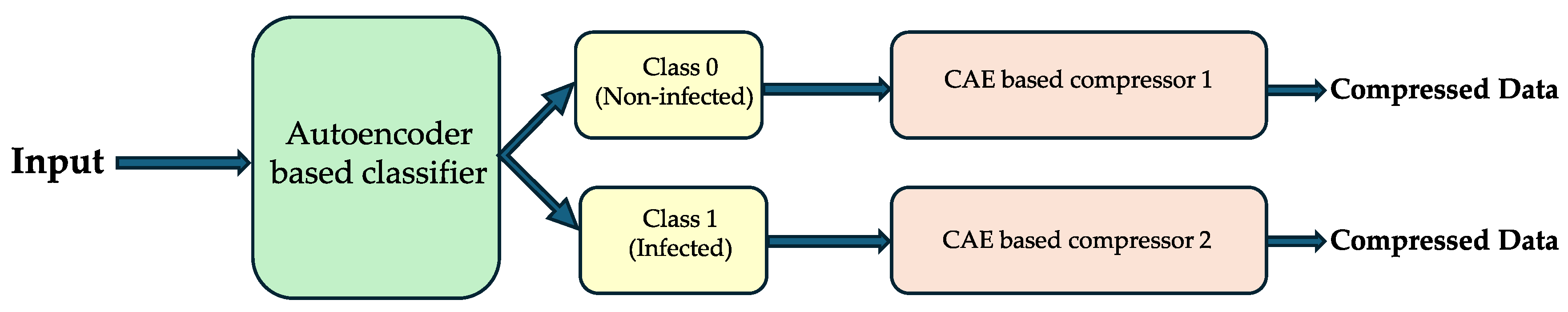
2.7. Proposed Joint Classification and Compression Approaches

2.7.1. Hybrid Model (Vision Transformer for Classification and Autoencoder for Compression)

We propose a hybrid model where the images in the dataset are first classified by using the vision transformer. To perform the task, all the images in the dataset were resized to a fixed input size that is suitable for the vision transformer (ViT) network. Next, random rotation, scaling, and horizontal flipping were applied to the training data to improve training and prevent overfitting. We used a pre-trained ViT network from MATLAB’s Computer Vision Toolbox that served as the backbone of the ViT model for pattern classification [53]. This model was originally trained on large and diverse datasets, which enables it to learn features in a generalized manner. These pre-learned features were used to improve the classification accuracy on our own dataset, eliminating the need to train the model from scratch.

There are two main parts of the pre-trained network: the backbone and the classification head. Features are extracted from the input images by the backbone of the network, whereas the classification head maps these features to the prediction score. To enable the neural network to classify the images over the classes in our dataset, we substituted the existing classification head with a new one that translates the extracted features into prediction scores for our new classes, as shown in Figure 4. After the introduction of the new head, the entire network was fine-tuned. In order to better capture the unique properties of our new dataset, the transformer’s weights were slightly modified during this procedure. The fine-tuning process employed a lower learning rate to prevent significant alteration in the pre-trained weights, enabling the model to adjust to new features while preserving its generalized feature extraction. The vision transformer (ViT) classifier was used to process the entire dataset, allowing the model to examine and classify every image according to the properties it had picked up during fine tuning. Next, we compressed the classified images by using the compressor described in Section 2.6.

2.7.2. Dual-Purpose Autoencoder Model (Autoencoders for Combined Classification and Compression)

In this section, the joint classification and compression method based on autoencoders is described. This method consists of a stacked autoencoder that is responsible for classification, followed by the CAE-based lossy compression architecture described in Section 2.6. The stacked autoencoder used for classification has two hidden layers that are trained individually in an unsupervised fashion. After that, a final softmax layer is trained, and the layers are joined to create a stacked network, which is then trained one last time by using supervised learning.

The prototype of the stacked network used for the purpose of classification is demonstrated in Figure 5. It starts with training a sparse autoencoder on the training data without utilizing the labels. This autoencoder uses regularizers such as L2WeightRegularization and SparsityRegularization to acquire sparse representation in the initial layer. The first parameter (L2WeightRegularization) governs the intensity of L2 regularization applied to the network’s weights [54]. SparsityRegularization manages the influence of a sparsity regularizer, which seeks to impose a limitation on the sparsity of the output generated by the hidden layer [54]. The first autoencoder generates a 1500-dimensional feature map that is a compact version of the input.

The second sparse autoencoder is also trained in a similar fashion. The only difference is that the features generated by the former encoder are used for training the second one. Also, there is a further dimension reduction to a 500-point vector, which is a more compressed representation of the original input. Finally, a softmax layer was used to classify the 500-dimensional feature vectors in a supervised fashion by using labels of the training data. After the completion of training of the three components (Autoencoder1, Autoencoder2, and softmax), the encoders from the autoencoders are combined along with the softmax layer to create a stacked network for classification purposes. The entire structure of joint classification and compression is depicted in Figure 6. The structure can be divided into two distinct parts: classifier and compressors. The detailed structure of the block titled “Autoencoder based classifier” is demonstrated in Figure 5. Conversely, the specifics of the “CAE-based compressors” are described in Section 2.6.

3. Results

In this section, we examine the effect of misclassification rates on overall compression efficiency. We start by evaluating the classification performance of both the autoencoder and vision transformer on the Malaria datasets. Subsequently, we compare the compression performance after feeding the classified data to our CAE-based compressor. Furthermore, we measure the compression performance of the CAE-based autoencoder by using the data that are correctly labeled, providing perspectives on how the accuracy of classification affects the overall results of compression.

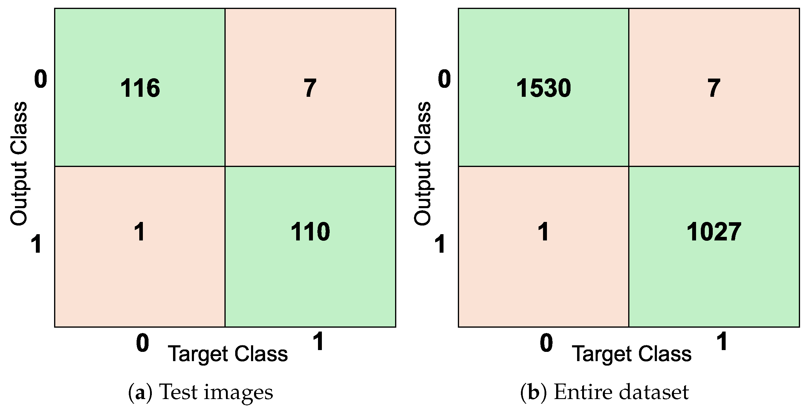
3.1. Evaluation of Classification Performance on UAB_Dataset

3.1.1. Autoencoder Results

The autoencoder used for classification was trained by using labeled training data from the UAB_Dataset. To test the performance of the model, we used 234 test images, which consist of equally sampled infected and non-infected cells. The autoencoders within the stacked network were trained with 1000 epochs, as was the softmax layer. After training the softmax layer, the entire stacked network was fine-tuned in a supervised fashion. The model was implemented in an environment with configuration 13th Gen Intel(R) Core(TM) i7-1365U, 1.80 GHz, 16 GB RAM, 64-bit, x64-based processor, and Windows 11 Pro OS using Matlab R2023b (64 bit). A confusion matrix was generated to demonstrate the classification performance of the stacked network on the test images, as shown in Figure 7a. The non-infected cells are represented as class 0, and the infected cells are presented as class 1. From the matrix, we can see that there are 116 instances in the top-left cell (Output Class 0, Target Class 0), indicating the number of instances the network accurately predicted as class 0. The top-right cell shows there are seven occurrences where the model incorrectly predicted the instances as class 0. The bottom-left cell has only one instance in the given matrix, which shows a single case where the model erroneously predicted class 0. The bottom-right cell represents the instances that were correctly classified by the model as class 1. This indicates that 110 items that truly belong to class 1 were correctly identified. The accuracy of the model on the test images is $96.6\%$.

Next, the entire dataset (training and testing) was passed through the autoencoder for classification. Figure 7b shows the performance of the autoencoder for the entire dataset. In our dataset, there are 1531 images of class 0 and 1034 images of class 1. We can observe that although some test images were erroneously classified, the model accurately predicted all the training images, resulting in the overall accuracy of $99.6\%$ for the entire dataset. The cells along the diagonal indicate the number of accurate predictions for each class, whereas the off-diagonal entries show the number of incorrect predictions, where one class was mistakenly predicted as the other. This matrix assists in assessing the effectiveness of a classification model, indicating how proficiently the model can differentiate between the two categories.

3.1.2. Vision Transformer Results

Figure 8 displays the confusion matrix that illustrates the effectiveness of the vision transformer in classifying images. For this purpose, we used the same test images that we used to evaluate the performance of the autoencoder model. The first matrix in Figure 8a showcases the model’s predictive accuracy focusing only on these test images. We can see that the architecture accurately predicted 112 non-Malaria cases and 115 Malaria-infected cases, representing an accuracy of $97\%$. When we passed the entire dataset (training and testing) through the model, we obtained an accuracy of $96.18\%$. Figure 8b shows that 20 Malaria-infected cases were misclassified as non-Malaria, whereas 78 normal cases were incorrectly predicted as infected. This means that unlike the autoencoder-based classifier, the vision transformer erroneously classified some of the images on which it was trained. The vision transformer model was implemented by using MATLAB 2024a (64 bit) on a system configured with an Intel Core(TM) i7-5930K CPU operating at 3.50 GHz, with 64 GB of RAM, and an NVIDIA GeForce GTX TITAN X Graphics Processing Unit (GPU) that includes 12 GB of memory.

3.2. Evaluation of Classification Performance on NIH_Dataset

3.2.1. Autoencoder Results

We adopted a similar stacked autoencoder architecture to that illustrated in Figure 5 to classify the NIH_Dataset. The primary modification for this dataset includes accommodating the increased dimensionality of the input images, which are four times larger than the images of the UAB_Dataset. So, each input to the autoencoder is a 10,000-dimensional vector, and the size of the hidden layers is 2500 and 1500. After training these layers in an unsupervised fashion, a softmax layer was added to the network and trained in a supervised fashion to produce the final classification output. All hyperparameter settings were identical to those described in Section 2.7.2. The performance of the classifier on the NIH_Dataset is summarized in Figure 9. From the confusion charts, we can see that the model achieved $95.03\%$ accuracy by correctly identifying 2619 instances out of 2756 instances on the test dataset. For the entire dataset, the model accurately predicted 27,037 cases out of 27,588 cases, corresponding to an accuracy of $98.1\%$. The results were obtained on the system described in Section 3.1.2.

3.2.2. Vision Transformer Results

The classification performance obtained from the vision transformer can be evaluated by analyzing the confusion charts that are present in Figure 10. The results were generated on the computational platform specified in Section 3.1.2. For the test images, the vision transformer misclassified 149 samples out of 2756 samples, showing an accuracy of $94.6\%$. On the entire dataset, the method erroneously predicted 1078 infected-cell images as uninfected and 313 normal-cell images as Malaria-infected, leading to an overall accuracy of $94.95\%$. While the autoencoder demonstrated slightly higher accuracy compared with the vision transformer, it can be stated that both models exhibited reliable performance on the NIH_Dataset. The impressive classification accuracy, even with greater diversity in the NIH_Dataset compared with the UAB_Dataset, highlights the robustness of our classifiers.

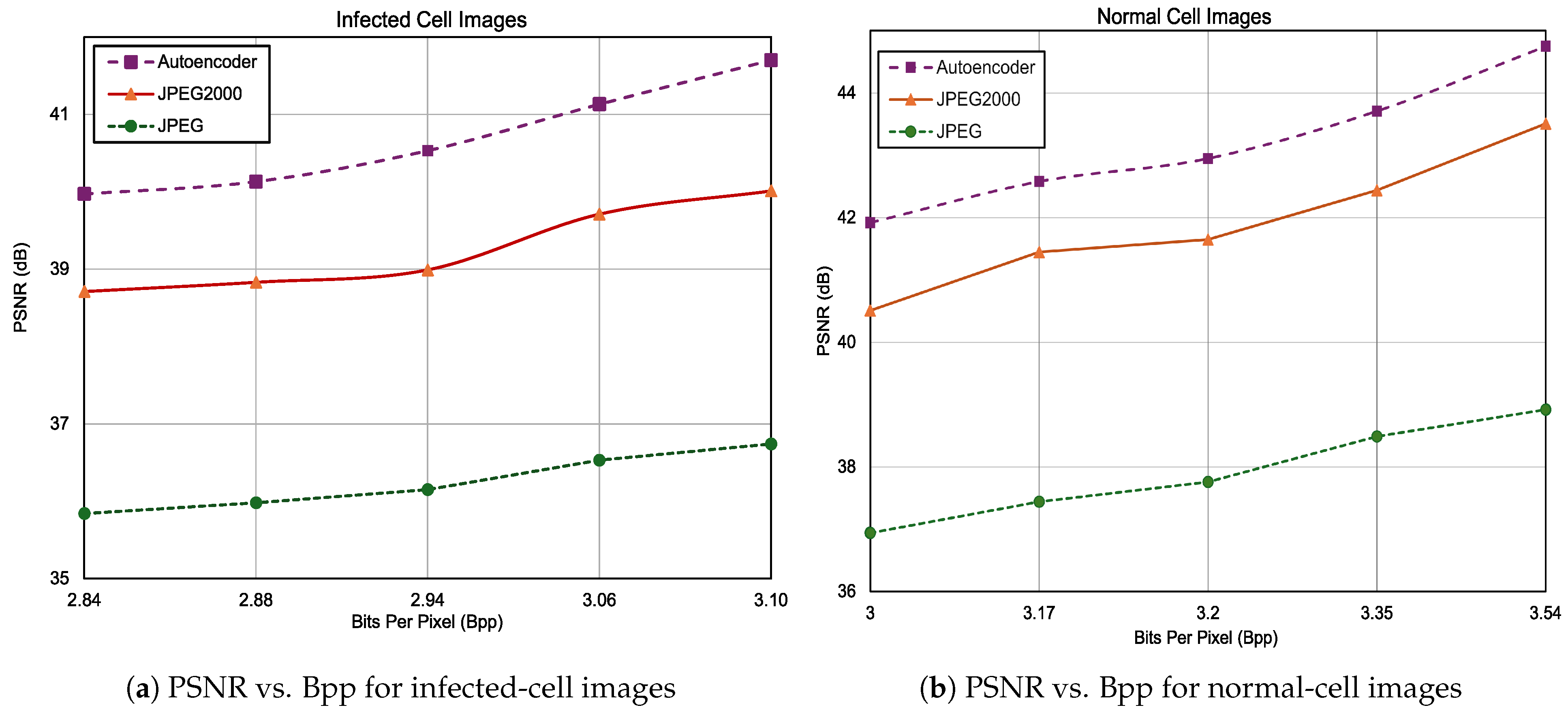
3.3. Compression Results on Precisely Labeled Data

3.3.1. UAB_Dataset

The UAB_Dataset was used for training the CAE-based autoencoder for compression. The dataset consists of accurately labeled data. We used two separate autoencoders for compression: one for the normal-cell images and the other for the infected-cell images. Two autoencoders were trained independently on the training data of the respective class. Since there are no misclassified data in the original dataset, the training was completed with only the data of the corresponding class on a system with the configuration described in Section 3.1.1 by using Python 3.12.3. After performing pre-processing, we trained each of the autoencoders for 1000 epochs with a batch size of 32. To minimize the error between the input and the reconstructed images, the model was compiled with the setup consisting of the Adam optimizer and mean square loss function. The choice of hyperparameters in our method was based on the combination of established norms in the field and experimental trials that demonstrated optimized performance for our model. Specifically, the Adam optimizer was selected due to its ability to dynamically modify learning rates, enhancing the ability of our model to efficiently converge. The values for batch size and the number of epochs were chosen to optimize computational efficiency while ensuring sufficient training cycles.

By using the compressed representation from the autoencoder and the residue, the average bits per pixel was calculated for each class (infected and normal) of images. Figure 11a,b show the superior performance of the CAE-based compressor against the traditional lossy compression techniques JPEG and JPEG 2000. The curves illustrate the trade-off in the compression in terms of bits per pixel (Bpp) and the reconstruction quality in terms of the Peak Signal-to-Noise Ratio (PSNR) for each technique. Bits per pixel (Bpp) quantifies the average number of bits encoded per pixel in an image, providing a measure of the compression level, and is calculated by using the formula in Equation (1). The PSNR can be defined by Equation (2), where MSE is the average squared pixel-by-pixel differences between the original and reconstructed images and MAX_PIXEL is the maximum pixel value of the image.

$$Bpp={\displaystyle \frac{\mathrm{image}\_\mathrm{file}\_\mathrm{size}\_\mathrm{in}\_\mathrm{bits}}{\mathrm{total}\_\mathrm{pixels}}}$$

(1)

$$\mathrm{PSNR}=20\times {log}_{10}\left({\displaystyle \frac{\mathrm{MAX}\_\mathrm{PIXEL}}{\sqrt{\mathrm{MSE}}}}\right)$$

(2)

In Figure 11a, we plotted the PSNR for different values of Bpp to compare the performance of each technique on infected-cell images. We can see from the graph that with the increase in Bpp values, the PSNR increases for each of the methods. It is evident that the CAE compressor reflects a strictly positive trend, whereas JPEG shows a flat line, depicting that the increase in Bpp has a minor impact on image quality. For any fixed value of Bpp, the reconstructed image generated by the CAE-based compressor is higher in quality compared with the other two counterparts. Overall, the CAE compressor yields superior image quality with equivalent compression settings, surpassing the JPEG 2000 approach, while JPEG has the lowest performance. The compressor encodes one image in 7 $\mathrm{m}$$\mathrm{s}$ seconds, whereas JPEG and JPEG2000 take 1 $\mathrm{m}$$\mathrm{s}$ and 4 $\mathrm{m}$$\mathrm{s}$, respectively.

In Figure 11b, PSNR vs. Bpp are plotted to evaluate the compression performance of the three methods on normal or non-infected cells. We can also see a similar trend in the trade-off between quality and compression for images of both categories. From Figure 11a,b, we can see that we need to spend more bits per pixel to achieve the same image quality for infected images compared with normal-cell images. Images of infected cells may naturally exhibit more intricate or diverse features because of the anomalies or alterations in cell structure resulting from infection. This increased complexity may require slightly higher bits per pixel (Bpp) to preserve image quality after compression, which explains the rise in Bpp for images of infected cells. The time the compressor takes to encode per test image is $8.2$ $\mathrm{m}$$\mathrm{s}$, while the time consumed by JPEG and JPEG2000 for conversion is 94 $\mathrm{\mu }$$\mathrm{s}$ and 3 $\mathrm{m}$$\mathrm{s}$, respectively.

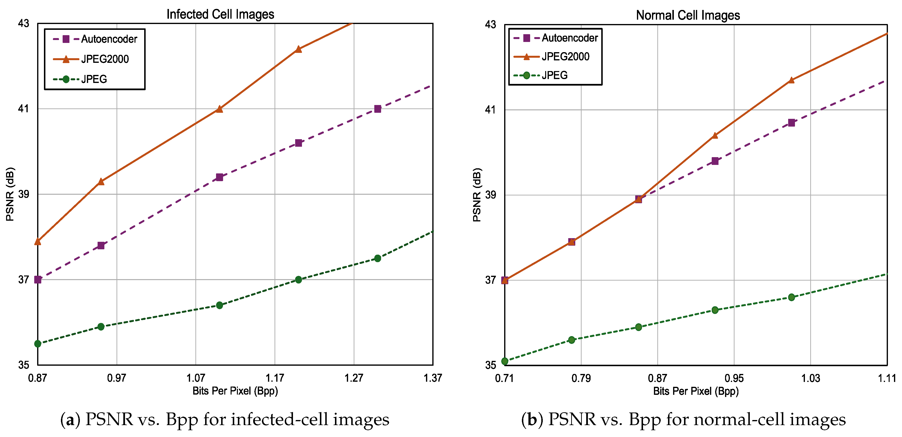
3.3.2. NIH_Dataset

The CAE-based autoencoder was trained on the NIH_Dataset to measure the compression performance of the model on this dataset. Images in the NIH_Dataset have twice the resolution of those in the UAB_Dataset. As a result, we had to adjust the pre-processing steps to handle the higher-resolution images of the dataset. The CAE framework illustrated in Figure 1 was modified slightly to accommodate these larger input images. Specifically, the resolution of the input images was upgraded to $100\times 100$, and the dense layers of the encoder and the decoder were scaled up to 200 and 40,000 neurons, respectively. Two separate CAE autoencoders were utilized, and each of them was trained on the images from a specific class: infected and non-infected. The training was performed by using the hyperparameter settings identical to those detailed in Section 3.3.1 and on the system specified in Section 3.1.2.

We derived the Bpp values for the images in the NIH_Dataset by using the encoded outputs of the CAE and plotted them against the PSNR in Figure 12. From the graphs, we can see that the proposed CAE model did not achieve satisfactory performance on this dataset. For the infected-cell images in Figure 12a, the model struggled to extract the shared features efficiently and demonstrated poor performance compared with JPEG2000. The underlying cause of this behavior is that the dataset showcases a significant amount of diversity, as the images were captured under various staining conditions and magnifications, including a wide variety of Malaria parasite stages. This variability adds difficulty in identifying reliable patterns, eventually impacting the performance of the model. The time taken by the compressor to encode one image is 40 $\mathrm{\mu }$$\mathrm{s}$, while JPEG2000 and JPEG take 7 $\mathrm{m}$$\mathrm{s}$ and 80 $\mathrm{\mu }$$\mathrm{s}$, respectively.

For normal-cell images, we see a clear trend in Figure 12b indicating that the performance of the CAE aligns with that of JPEG2000 for lower BPP values. Precisely, for BPP values lower than 0.85, the model achieves similar PSNR values to JPEG2000 by spending an equivalent number of bits. The similarity in performance at reduced BPP values suggests that the CAE model effectively captures the simpler, more general features from normal-cell images. However, when the BPP increases, the model shows lower performance than JPEG2000, possibly because CAE has to focus on more diverse and detailed features to effectively reconstruct the images at comparable quality. The graphs in Figure 12a,b show an increasing trend in the PSNR with the increase in BPP values. Moreover, the model outperformed JPEG across both infected and non-infected cases for both normal and infected images. The time consumed by the CAE, JPEG200, and JPEG to encode one single image is 42 $\mathrm{\mu }$$\mathrm{s}$, $6.5$ $\mathrm{m}$$\mathrm{s}$, and 72 $\mathrm{\mu }$$\mathrm{s}$, respectively. Interestingly, for the NIH_Dataset, the models spend fewer bits per pixel than for the UAB_Dataset. The NIH_Dataset has images at higher resolution, which means that the images include more repetitive and smooth areas compared with the images of the UAB_Dataset. The existence of more uniform color and texture decreases the degree of complexity the encoder has to handle, which results in compressing the higher-resolution images in the NIH_Dataset at a lower bit rate.

4. Discussion

Quantitative Analysis: How Classification Accuracy Influences Compression

This section provides a comprehensive analysis of the influence of misclassification on compression performance.

Table 1. Comparison of compression techniques in terms of average Bpp and PSNR for normal-cell images.

Dataset	Method	Accuracy	BPP	PSNR (dB)
UAB_Dataset	CAE-based compressor	100%	2.90	41.35
	Dual-purpose autoencoder	99.6%	2.91	41.20
	Hybrid model	96.18%	2.92	41.20
	JPEG2000	–	3.10	41.09
	JPEG	–	3.97	40.73
NIH_Dataset	CAE-based compressor	100%	0.85	38.9
	Dual-purpose autoencoder	98.1%	0.87	38.5
	Hybrid model	94.95%	0.87	38
	JPEG2000	–	0.85	38.9
	JPEG	–	1.35	38.5

and

Table 2. Comparison of compression techniques in terms of average Bpp and PSNR for infected-cell images.

Dataset	Method	Accuracy	BPP	PSNR
UAB_Dataset	CAE-based compressor	100%	2.90	40.58
	Dual-purpose autoencoder	99.6%	2.92	40.56
	Hybrid model	96.18%	2.92	40.47
	JPEG2000	–	3.10	40.01
	JPEG	–	4.00	39.82
NIH_Dataset	CAE-based compressor	100%	0.95	37.8
	Dual-purpose autoencoder	98.1%	0.95	37
	Hybrid model	94.95%	0.96	36.87
	JPEG2000	–	0.87	37.9
	JPEG	–	1.2	37

present a comparative analysis of different image compression methods applied on the UAB_Dataset and NIH_Dataset. The comparison is based on two performance parameters: bits per pixel (Bpp) and Peak Signal-to-Noise Ratio (PSNR), assessed for both normal- and infected-cell images.

The best performance for the UAB_Dataset is obtained when the CAE-based compressor is trained on precisely labeled data, as shown in Table 1. Even when utilizing data that have been categorized by different models, like a stacked autoencoder or a vision transformer, the CAE continues to perform exceptionally well, with only a minor reduction in performance as the accuracy of classification declines. Interestingly, the conventional compression approaches (JPEG and JPEG 2000) exhibit inferior performance compared with the CAE-based compression technique, despite the CAE being trained on some misclassified data from autoencoder-based and vision transformer-based classifiers. When applying the CAE-based compressor on the NIH_Dataset, we observed that the method showed similar performance as JPEG2000 when we trained the model without any misclassified data. The performance of the CAE was compromised, as we trained the model with a training set that contained misclassified data.

Table 2 concentrates on infected-cell images, showcasing the performance of the same compression techniques as Table 1. The outcomes exhibit a similar pattern to what was seen with normal-cell images for the UAB_Dataset, with minor differences in Bpp and PSNR values among the techniques. The CAE is capable of learning relevant features efficiently, which results in better performance in terms of Bpp and PSNR. In contrast, generic methods like JPEG and JPEG 2000 spend more bits per pixel but fail to generate images of comparable quality. Contrary to the UAB_Dataset, the NIH_Datset reveals a different performance pattern. Here, JPEG2000 appears to be a more suitable compression method than the CAE. The difference arises due to the CAE’s reliance on leveraging common features among diverse infected-cell images. In contrast, JPEG2000 uses its wavelet transformation technique and independently processes each image without necessitating any commonalities among the images. The results obtained on the NIH_Dataset underscore the necessity of uniform feature distribution across the dataset to attain a desirable compression rate by using the CAE-based compressor.

The above results show that classification directly influences the efficacy of compression. As we compared the CAE-based autoencoder performance on different datasets with different levels of precision, the link between classification accuracy and compression efficiency became clear. It is notable that even minor deviations in classification accuracy can subtly impact the compression rate. The CAE trained on accurately classified data from the UAB_Dataset reaches a Bpp value of 2.90 and serves as a baseline of the optimum compression performance for normal-cell images, with the PSNR being 41.35 dB. There is a slight rise in Bpp, as the accuracy of classification declines. In particular, by using 99.6% accurately classified data, the Bpp value experiences a slight increase of about 0.34% to 2.91. When the classification accuracy drops to 96.18%, the Bpp reaches 2.92, albeit failing to generate the same reconstructed image quality, as evident from the low PSNR value. The presence of misclassified images in the training dataset leads to increased Bpp and a lower Peak Signal-to-Noise Ratio. The same phenomenon is also evident for the NIH_Dataset, as the overall efficiency of the compression diminishes as the classification performance decreases.

The data in Table 2 reveal the influence of classification accuracy on compression for infected images, which mirrors the trends we have observed in normal-cell images. The CAE trained on appropriately labeled data from the UAB_Dataset continues to outperform others in preserving the highest quality, with a PSNR of 40.58 dB with a Bpp value of 2.90. When trained on slightly misclassified data generated from the autoencoder or vision transformer, the CAE produced compressed images with a Bpp value of 2.92. Although using the autoencoder-classified data, the CAE could achieve reconstruction image quality similar to the perfectly classified case. A slight decrement in PSNR was noticed for the data classified by the vision transformer to a level of 40.47 dB, demonstrating a minor but noticeable impact of reduced classification accuracy. The correlation between classification accuracy and compression rate is also apparent in the NIH_Dataset for infected-cell images. The CAE achieves a quality of 37.8 dB at 2.90 BPP with $100\%$ accurate data. The quality decreases to 37 dB while training with minor misclassifications from the classifier with an accuracy of $98.1\%$.

The crucial balance between accuracy in classification and efficiency in compression is highlighted by the comparative analysis of the compression methods. It can be said that maintaining the integrity of data plays a crucial role in the performance of our proposed compression method. Specifically, higher classification accuracy can effectively boost the compressor performance while preserving the quality of the reconstructed image. Additionally, the compression rate is enhanced by the existence of shared features among the images within the dataset. The need for the selection of a suitable classification model is demonstrated in the comparative analysis. The study also provides quantitative measures of the impact of classification accuracy on compression efficacy.

The medical sector can benefit greatly from the findings of this study, especially when it comes to efficiently transferring and storing high-resolution images. The proposed CAE-based compression architectures allow healthcare systems to improve their image storage efficiency while maintaining the high image quality necessary for precise medical analysis and diagnosis. This method shows potential for numerous medical imaging applications, such as digital pathology, radiology, and others, where accurate diagnoses depend on high-resolution images that usually need a significant amount of storage space. Furthermore, the possibility of utilizing this technology in telemedicine is considerable, particularly in areas with restricted bandwidth, to enhance access to quality healthcare services.

5. Limitations and Future Research Directions

The findings of this research study provide promising insights into the UAB_Dataset, yet it is important to acknowledge the limitations associated with this particular dataset, which focuses exclusively on a certain type of cell images. This narrow focus limits the generalization capacity of the model. The compression efficiency of the CAE is compromised when implemented on the NIH_Dataset, with varying diversity and scale. To strengthen the validity of our model, future studies should include various medical imaging domains, covering different categories of cells and possibly other medical circumstances. It remains to be seen if the results obtained herein can be generalized to much larger datasets used in other domains. To this end, data augmentation can be used to increase the diversity of our dataset [48]. In further research, we will consider datasets with more image patterns. We hypothesize that further subdividing the images into more classes would lead to additional gains in overall compression performance.

6. Conclusions

In this paper, we proposed two deep learning models for the joint classification and compression of red blood cell images used for automated Malaria infection detection. The results highlight the importance of attaining high classification accuracy in order to achieve good compression efficiency. We trained two distinct deep learning classification models on the same dataset and measured their accuracy. The classified data from each model were then used to train a deep learning-based image compression method. Compared with the baseline model, the hybrid model performs slightly less optimally in terms of classification accuracy and compression efficacy. This study emphasizes the necessity of higher classification accuracy to achieve desirable compression, as we can see that compression performance suffers with the decrease in accuracy. This study also demonstrates that the proposed joint pattern classification and data compression scheme using deep learning can outperform traditional lossy compression techniques in terms of both quality and compressed bit rates. The scheme can find applications in the remote diagnosis of Malaria infection, as the excellent rate/distortion trade-offs would facilitate the quick transmission of whole-slide images while guaranteeing sufficient reconstruction quality. In areas where the confidentiality of data is the main concern, the joint classification and compression scheme can also be beneficial, since the data will be securely transmitted in a coded form. The coded data can only be recovered with the knowledge of the decoder architecture.

References

- Centers for Disease Control and Prevention. Malaria’s Impact Worldwide; Centers for Disease Control and Prevention: Atlanta, GA, USA, 2024.
- World Health Organization. World Malaria Report 2023; World Health Organization: Geneva, Switzerland, 2023. [Google Scholar]
- Bronzan, R.N.; McMorrow, M.L.; Patrick Kachur, S. Diagnosis of malaria: Challenges for clinicians in endemic and non-endemic regions. Mol. Diagn. Ther. 2008, 12, 299–306. [Google Scholar] [CrossRef] [PubMed]
- Delahunt, C.B.; Gachuhi, N.; Horning, M.P. Metrics to guide development of machine learning algorithms for malaria diagnosis. Front. Malar. 2024, 2, 1250220. [Google Scholar] [CrossRef]
- Hoyos, K.; Hoyos, W. Supporting Malaria Diagnosis Using Deep Learning and Data Augmentation. Diagnostics 2024, 14, 690. [Google Scholar] [CrossRef]
- Ikerionwu, C.; Ugwuishiwu, C.; Okpala, I.; James, I.; Okoronkwo, M.; Nnadi, C.; Orji, U.; Ebem, D.; Ike, A. Application of machine and deep learning algorithms in optical microscopic detection of Plasmodium: A malaria diagnostic tool for the future. Photodiagn. Photodyn. Ther. 2022, 40, 103198. [Google Scholar] [CrossRef]
- Siłka, W.; Wieczorek, M.; Siłka, J.; Woźniak, M. Malaria detection using advanced deep learning architecture. Sensors 2023, 23, 1501. [Google Scholar] [CrossRef]
- Marques, G.; Ferreras, A.; de la Torre-Diez, I. An ensemble-based approach for automated medical diagnosis of malaria using EfficientNet. Multimed. Tools Appl. 2022, 81, 28061–28078. [Google Scholar] [CrossRef]
- Loh, D.R.; Yong, W.X.; Yapeter, J.; Subburaj, K.; Chandramohanadas, R. A deep learning approach to the screening of malaria infection: Automated and rapid cell counting, object detection and instance segmentation using Mask R-CNN. Comput. Med. Imaging Graph. 2021, 88, 101845. [Google Scholar] [CrossRef] [PubMed]
- Alkhaldi, T.M.; Hashim, A.N. Automatic Detection of Malaria Using Convolutional Neural Network. Math. Stat. Eng. Appl. 2022, 71, 939–947. [Google Scholar]
- Li, S.; Du, Z.; Meng, X.; Zhang, Y. Multi-stage malaria parasite recognition by deep learning. GigaScience 2021, 10, giab040. [Google Scholar] [CrossRef]
- Islam, M.S.B.; Islam, J.; Islam, M.S.; Sumon, M.S.I.; Nahiduzzaman, M.; Murugappan, M.; Hasan, A.; Chowdhury, M.E. Development of Low Cost, Automated Digital Microscopes Allowing Rapid Whole Slide Imaging for Detecting Malaria. In Surveillance, Prevention, and Control of Infectious Diseases: An AI Perspective; Springer: Berlin/Heidelberg, Germany, 2024; pp. 73–96. [Google Scholar]
- Saxena, S.; Sanyal, P.; Bajpai, M.; Prakash, R.; Kumar, S. Trials and tribulations: Developing an artificial intelligence for screening malaria parasite from peripheral blood smears. Med J. Armed Forces India, 2023; in press. [Google Scholar]
- Pan, W.D.; Dong, Y.; Wu, D. Classification of malaria-infected cells using deep convolutional neural networks. In Machine Learning: Advanced Techniques and Emerging Applications; IntechOpen: London, UK, 2018; Volume 159. [Google Scholar]
- Valente, J.; António, J.; Mora, C.; Jardim, S. Developments in image processing using deep learning and reinforcement learning. J. Imaging 2023, 9, 207. [Google Scholar] [CrossRef]
- Mishra, D.; Singh, S.K.; Singh, R.K. Deep architectures for image compression: A critical review. Signal Process. 2022, 191, 108346. [Google Scholar] [CrossRef]
- Yasin, H.M.; Abdulazeez, A.M. Image compression based on deep learning: A review. Asian J. Res. Comput. Sci. 2021, 8, 62–76. [Google Scholar] [CrossRef]
- Bourai, N.E.H.; Merouani, H.F.; Djebbar, A. Deep learning-assisted medical image compression challenges and opportunities: Systematic review. Neural Comput. Appl. 2024, 36, 10067–10108. [Google Scholar] [CrossRef]
- Dimililer, K. DCT-based medical image compression using machine learning. Signal Image Video Process. 2022, 16, 55–62. [Google Scholar] [CrossRef]
- Abd-Alzhra, A.S.; Al-Tamimi, M.S. Image compression using deep learning: Methods and techniques. Iraqi J. Sci. 2022, 63, 1299–1312. [Google Scholar] [CrossRef]
- Yang, E.H.; Amer, H.; Jiang, Y. Compression helps deep learning in image classification. Entropy 2021, 23, 881. [Google Scholar] [CrossRef]
- Silva, J.M.; Almeida, J.R. Enhancing metagenomic classification with compression-based features. Artif. Intell. Med. 2024, 156, 102948. [Google Scholar] [CrossRef] [PubMed]
- Chang, C.I.; Liang, C.C.; Hu, P.F. Iterative Gaussian–Laplacian Pyramid Network for Hyperspectral Image Classification. IEEE Trans. Geosci. Remote Sens. 2024, 62, 5510122. [Google Scholar] [CrossRef]
- Barsi, A.; Nayak, S.C.; Parida, S.; Shukla, R.M. A deep learning-based compression and classification technique for whole slide histopathology images. Int. J. Inf. Technol. 2024, 16, 4517–4526. [Google Scholar] [CrossRef]
- Hamano, G.; Imaizumi, S.; Kiya, H. Effects of JPEG Compression on Vision Transformer Image Classification for Encryption-then-Compression Images. Sensors 2023, 23, 3400. [Google Scholar] [CrossRef]
- Liu, L.; Chen, T.; Liu, H.; Pu, S.; Wang, L.; Shen, Q. 2C-Net: Integrate image compression and classification via deep neural network. Multimed. Syst. 2023, 29, 945–959. [Google Scholar]
- Hurwitz, J.; Nicholas, C.; Raff, E. Neural Normalized Compression Distance and the Disconnect Between Compression and Classification. arXiv 2024, arXiv:2410.15280. [Google Scholar]
- Xie, W.; Fan, X.; Zhang, X.; Li, Y.; Sheng, M.; Fang, L. Co-compression via superior gene for remote sensing scene classification. IEEE Trans. Geosci. Remote Sens. 2023, 61, 5604112. [Google Scholar] [CrossRef]
- Dong, Y.; Pan, W.D.; Wu, D. Impact of misclassification rates on compression efficiency of red blood cell images of malaria infection using deep learning. Entropy 2019, 21, 1062. [Google Scholar] [CrossRef]
- Pintelas, E.; Livieris, I.E.; Pintelas, P.E. A Convolutional Autoencoder Topology for Classification in High-Dimensional Noisy Image Datasets. Sensors 2021, 21, 7731. [Google Scholar] [CrossRef] [PubMed]
- Cheng, Z.; Sun, H.; Takeuchi, M.; Katto, J. Deep Convolutional AutoEncoder-based Lossy Image Compression. In Proceedings of the 2018 Picture Coding Symposium (PCS), Francisco, CA, USA, 24–27 June 2018; pp. 253–257. [Google Scholar] [CrossRef]
- Ismail, A.R.; Zulhazmi Rafiqi Azhary, M.; Zaharin Noor Azwan, N.A.; Ismail, A.; Alsaiari, N.A. Performance Evaluation of Medical Image Denoising using Convolutional Autoencoders. In Proceedings of the 2024 3rd International Conference on Creative Communication and Innovative Technology (ICCIT), Tangerang, Indonesia, 7–8 August 2024; pp. 1–6. [Google Scholar] [CrossRef]
- Han, K.; Wang, Y.; Chen, H.; Chen, X.; Guo, J.; Liu, Z.; Tang, Y.; Xiao, A.; Xu, C.; Xu, Y.; et al. A Survey on Vision Transformer. IEEE Trans. Pattern Anal. Mach. Intell. 2023, 45, 87–110. [Google Scholar] [CrossRef]
- Omer, A.A.M. Image Classification Based on Vision Transformer. J. Comput. Commun. 2024, 12, 49–59. [Google Scholar] [CrossRef]
- Dosovitskiy, A.; Beyer, L.; Kolesnikov, A.; Weissenborn, D.; Zhai, X.; Unterthiner, T.; Dehghani, M.; Minderer, M.; Heigold, G.; Gelly, S.; et al. An Image is Worth 16x16 Words: Transformers for Image Recognition at Scale. arXiv 2021, arXiv:2010.11929. [Google Scholar]
- Carion, N.; Massa, F.; Synnaeve, G.; Usunier, N.; Kirillov, A.; Zagoruyko, S. End-to-End Object Detection with Transformers. In Computer Vision—ECCV 2020; Springer: Cham, Switzerland, 2020; pp. 213–229. [Google Scholar] [CrossRef]
- Shivappriya, S.N.; Harikumar, R. Performance Analysis of Deep Neural Network and Stacked Autoencoder for Image Classification. In Computational Intelligence and Sustainable Systems: Intelligence and Sustainable Computing; Anandakumar, H., Arulmurugan, R., Onn, C.C., Eds.; Springer International Publishing: Cham, Switzerland, 2019; pp. 1–16. [Google Scholar] [CrossRef]
- Elngar, A.A.; Arafa, M.; Fathy, A.; Moustafa, B.; Mahmoud, O.; Shaban, M.; Fawzy, N. Image classification based on CNN: A survey. J. Cybersecur. Inf. Manag. 2021, 6, 18–50. [Google Scholar]
- Zhao, Z.Q.; Zheng, P.; Xu, S.T.; Wu, X. Object Detection With Deep Learning: A Review. IEEE Trans. Neural Networks Learn. Syst. 2019, 30, 3212–3232. [Google Scholar] [CrossRef]
- Maurício, J.; Domingues, I.; Bernardino, J. Comparing Vision Transformers and Convolutional Neural Networks for Image Classification: A Literature Review. Appl. Sci. 2023, 13, 5521. [Google Scholar] [CrossRef]
- Fraihat, S.; Al-Betar, M.A. A novel lossy image compression algorithm using multi-models stacked AutoEncoders. Array 2023, 19, 100314. [Google Scholar] [CrossRef]
- Gogoi, M.; Begum, S.A. Image Classification Using Deep Autoencoders. In Proceedings of the 2017 IEEE International Conference on Computational Intelligence and Computing Research (ICCIC), Coimbatore, India, 14–16 December 2017; pp. 1–5. [Google Scholar] [CrossRef]
- Rao, K.R.; Domínguez, H.O. JPEG Series; CRC Press: Boca Raton, FL, USA, 2022. [Google Scholar]
- Sayood, K. Introduction to Data Compression; Morgan Kaufmann: Burlington, MA, USA, 2017. [Google Scholar]
- Jamil, S.; Piran, M.J.; MuhibUrRahman. Learning-Driven Lossy Image Compression; A Comprehensive Survey. arXiv 2022, arXiv:2201.09240. [Google Scholar]
- Valenzise, G.; Purica, A.; Hulusic, V.; Cagnazzo, M. Quality Assessment of Deep-Learning-Based Image Compression. In Proceedings of the 2018 IEEE 20th International Workshop on Multimedia Signal Processing (MMSP), Vancouver, BC, Canada, 29–31 August 2018; pp. 1–6. [Google Scholar] [CrossRef]
- Mishra, D.; Singh, S.K.; Singh, R.K. Lossy medical image compression using residual learning-based dual autoencoder model. In Proceedings of the 2020 IEEE 7th Uttar Pradesh Section International Conference on Electrical, Electronics and Computer Engineering (UPCON), Prayagraj, India, 27–29 November 2020; pp. 1–5. [Google Scholar]
- Dong, Y.; Jiang, Z.; Shen, H.; David Pan, W.; Williams, L.A.; Reddy, V.V.B.; Benjamin, W.H.; Bryan, A.W. Evaluations of deep convolutional neural networks for automatic identification of malaria infected cells. In Proceedings of the 2017 IEEE EMBS International Conference on Biomedical & Health Informatics (BHI), Orland, FL, USA, 16–19 February 2017; pp. 101–104. [Google Scholar] [CrossRef]
- Dataset Used in This Paper. Available online: http://www.ece.uah.edu/~dwpan/malaria_dataset/ (accessed on 3 January 2025).
- National Library of Medicine. Malaria Datasheet—Image Processing Research. 2025. Available online: https://lhncbc.nlm.nih.gov/LHC-research/LHC-projects/image-processing/malaria-datasheet.html (accessed on 2 March 2025).
- Ioffe, S.; Szegedy, C. Batch Normalization: Accelerating Deep Network Training by Reducing Internal Covariate Shift. arXiv 2015, arXiv:1502.03167. [Google Scholar]
- Theis, L.; Shi, W.; Cunningham, A.; Huszár, F. Lossy Image Compression with Compressive Autoencoders. arXiv 2017, arXiv:1703.00395. [Google Scholar]
- MathWorks. Train Vision Transformer Network for Image Classification. Available online: https://www.mathworks.com/help/deeplearning/ug/train-vision-transformer-network-for-image-classification.html (accessed on 31 January 2023).
- Goodfellow, I.; Bengio, Y.; Courville, A. Deep Learning; MIT Press: Cambridge, MA, USA, 2016; Available online: http://www.deeplearningbook.org (accessed on 3 January 2025).