Article

A Machine Learning Evaluation of the Impact of Bit-Depth for the Detection and Classification of Wireless Interferences in Global Navigation Satellite Systems

by
Gianmarco Baldini
1,* and
Fausto Bonavitacola
2
1
European Commission, Joint Research Centre, 21027 Ispra, Italy
2
Piksel, 20126 Milan, Italy
*
Author to whom correspondence should be addressed.
Electronics 2025, 14(6), 1147; https://doi.org/10.3390/electronics14061147
Submission received: 22 January 2025 / Revised: 11 March 2025 / Accepted: 12 March 2025 / Published: 14 March 2025

Abstract

:
The performance of the services provided by Global Navigation Satellite Systems (GNSSs) can be seriously degraded by the presence of wireless interferences, and Machine Learning (ML) has been applied to address this problem using the digital artifacts generated by the GNSS receiver. While such an application is not novel in the literature, the analysis of the impact of the bit-depth at which the GNSS signal is recorded has not received significant attention. The type and power level of the wireless interference are also important factors to investigate in this context. This paper addresses this gap by performing an extensive analysis of the impact of these factors on a data set of GNSS signals subject to three different types of wireless interferences with ML and DL algorithms. The analysis is a combination of a pre-processing phase where the Carrier-to-Noise Ratio (CNR) values of different satellites are evaluated, the extraction of relevant features for ML, and the application of a Convolutional Neural Network (CNN) with a multi-head attention layer. The results show that the proposed approach is able to detect the presence of interference with great accuracy (e.g., 99%) but the type of interference and bit-depth can decrease the performance.

1. Introduction

Global Navigation Satellite System (GNSS) technologies are used in many applications in the modern world from the automotive domain to the provision of Location-Based Services (LBSs), synchronization of cellular networks, and so on. Such applications set the need for delivering high-performance GNSS solutions in terms of performance parameters, such as accuracy, availability, continuity, and integrity [1].
On the other hand, GNSS signals may be vulnerable to either intentional or unintentional Radio Frequency Interference (RFI) due to their weak received power and the wide availability of low-cost jammers [2,3]. In particular, jamming is an intentional RFI aimed to disrupt GNSS-based services by deliberately transmitting powerful signals in GNSS bands. It would be useful to characterize the type of jamming attack to apply appropriate mitigation measures.
As in other fields, Machine Learning (ML) and Deep Learning (DL) have been increasingly used in GNSSs to address a number of problems including the detection of ionospheric disturbances, scenario classification [1], and so on. In parallel, ML and DL were used to detect and classify types of disturbances like interference in wireless communications [4] or power quality disturbances in power transmission systems [5].
The underlying concept of this paper is to apply ML and DL algorithms to the detection and classification of interferences of GNSSs taking into consideration the specific aspects of the GNSS context: (1) the digital observables identified with the Carrier-to-Noise Ratio (CNR) from the GNSS receivers are the result of a pre-processing step where discriminating information of the wireless interferences may be lost, (2) GNSS satellites may not be fully visible at the time of the data acquisition and processing, which can also obfuscate important information on the interferences, and (3) the signal may be processed using different bit-depths as there is a trade-off between processing time and storage.
The aim of this paper is to investigate the application both of ‘shallow’ (e.g., Decision Tree) and neural networks ‘deep’ ML algorithms to detect and classify different types of wireless interferences in GNSS data collected from real measurements and processed at different power levels and bit-depths. Additional details on the novelty and advancement of this study in comparison to the state of the art in the research literature are provided at the end of Section 2.
The structure of this paper is the following: Section 2 provides a literature review on the application of ML and DL to the problem of detection and classification of wireless interference in GNSS signals. Section 3 outlines the overall methodology used for the implementation of data collection, pre-processing, and the application of the ML and DL algorithms. In particular, Section 3.2 describes the ML and DL algorithms used to perform the detection and classification including the Convolutional Neural Network (CNN) architecture and the features used in the ML application. Section 4 describes the data set used to evaluate the approach. The data set was generated by the authors in their laboratory and it will be available to the research community after the publication of the paper. Section 5 provides the results of the comprehensive analysis of the application of the proposed approach on the data set for different values of the hyper-parameters (e.g., number of considered satellites) and the types of wireless interference. Finally, Section 6 concludes the paper and outlines potential future developments.

2. Related Work

This section provides an overview on the related work on the detection and identification of wireless interferences in GNSS signals. Section 2.1 gives an overview on the application of ML to this problem while Section 2.2 reports on the literature where neural networks including DL are applied.

2.1. Related Work on Machine Learning

An extensive survey on the application of ML and DL to GNSS problems is given in [1], where the detection of interference is one of the considered sub-cases among others (estimate of ionospheric effects, signal detection, positioning), and it is often associated with jamming detection and classification. One of the first studies, which applied ML to jamming identification and classification is [6] where a twin Support Vector Machine (SVM) algorithm (TWSVM) was used for real-time interference monitoring. The TWSVM is the preferred SVM for improved classification performance. In contrast, DL algorithms were not used and the impact of the bit-depth was not considered at all. Another paper, which used shallow Machine Learning algorithms was [7], which adopted a combination of SVM and Principal Component Analysis (PCA) to reduce the feature space. The goal of the authors of [7] was to detect both jamming and spoofing attacks. However, DL was not used. Several recent papers have adopted DL algorithms, demonstrating in general a superior performance to shallow Machine Learning algorithms in this context as discussed in the next sub-section.

2.2. Related Work on Neural Networks and Deep Learning

The authors in [8] adopted a CNN (as in this paper) to classify different types of jamming signals present in GNSS bands. In particular, pulse jamming, narrowband, and wideband chirp jamming were used to generate the jamming signals. As in this study, different power levels were also used. The main difference of this paper with [8] is that the analysis with CNNs is performed directly on the radio frequency space in [8], while in this study the CNR values are used. The approach in this paper is more realistic because the classification of the interferences in the original radio frequency space would require an additional spectrum analyzer component, while the CNR values (as C / N 0 time series) are provided even by consumer-grade GNSS receivers. Apart from this significant difference, the authors of [8] do not take into consideration the impact of the bit-depth. The authors of [9] have also used a CNN with a similar limitation that the DL algorithm is applied directly to the spectrograms of the combined GNSS and jamming signals, which can also be computing-intensive due to the need to generate the spectrograms from the signal in space. The jamming signals used in [9] are chirp-based, pulse, or narrowband signals, which are similar to the ones used in this paper. The results of [9] show that SVM achieves better accuracy than the CNN, whereas this study obtained opposite results. Furthermore, it should be taken in consideration that this study used a more sophisticated CNN architecture with a multi-head attention layer rather than the baseline two-layer CNN architecture proposed in [9]. A similar approach was also followed in [10] with a CNN architecture and [11], where DL algorithms (i.e., ResNet18 and Transformers) were applied both to the time domain and spectral domain representation of the combination of the GNSS signal and the interferences. Pulse, chirp, and modulated signals were used to generate the interference. An evolution of these approaches is to use combinations of time frequency transforms as in [12], where the Wigner-Ville transform (WVT) and the spectrograms were used in combination to identify and classify interferences in GNSSs using a CNN. The studies [10,11,12] have the same limitation as the previous papers because the application of the CNN to the original signal or its spectral domain (either with Fast Fourier Transform (FFT) or with Time Frequency (TF)) does not take into consideration the processing (e.g., signal correlation) of the GNSS receiver and it would require additional components. The bit-depth aspect was also not considered. A similar use of spectrogram and WVT and CNN was adopted in [13], while the authors of [3] applied more sophisticated DL algorithms and architectures than a vanilla CNN for the classification of interference, but again the spectrogram was used and no analysis on bit-depth was performed. Regarding the use of C / N 0 instead of spectrograms, the authors in [14] analyzed the impact of jamming signals with different levels of power on the C / N 0 but the bit-depth was not considered and no classification attempt with ML or DL was made.
We summarize in the following bullet list the key contributions and advancements of this paper in comparison to the reviewed literature:
  • With a good degree of novelty, the CNN is applied to the C / N 0 digital artifacts created by the GNSS receiver instead of the spectral domain representation of the signal in space. Even if the application of the CNN to the C / N 0 observables may be more challenging because the original Radio Frequency (RF) signal is pre-processed and some information could be lost, the approach is more practical and realistic because it relies only on the output of the GNSS receiver and no additional components (e.g., spectrum analyzer) are needed.
  • For the first time in the literature, the impact of the bit-depth storage and reproduction of the original GNSS signal is evaluated in combination with CNN and the C / N 0 artifacts for the problem of detection and classification of interferences in GNSSs.
  • A CNN with a multi-head attention layer is used for classification, which is more sophisticated than the CNN architectures used in the literature so far.
  • The authors have produced a novel (because it is based on C / N 0 data) and comprehensive data set with different types of interference, levels of attenuation, and bit-depths, which was not made available before to the research community. This data set will be available after the publication of the manuscript.

3. Methodology

This section describes the approach used in this study to detect and classify the different types of interference. In particular, Section 3.1 describes the overall set of procedures and how they are integrated among them. Section 3.2 describes the ML algorithms while Section 3.3 describes the CNN architecture and related hyper-parameters. Section 3.4 describes the metrics of evaluation.

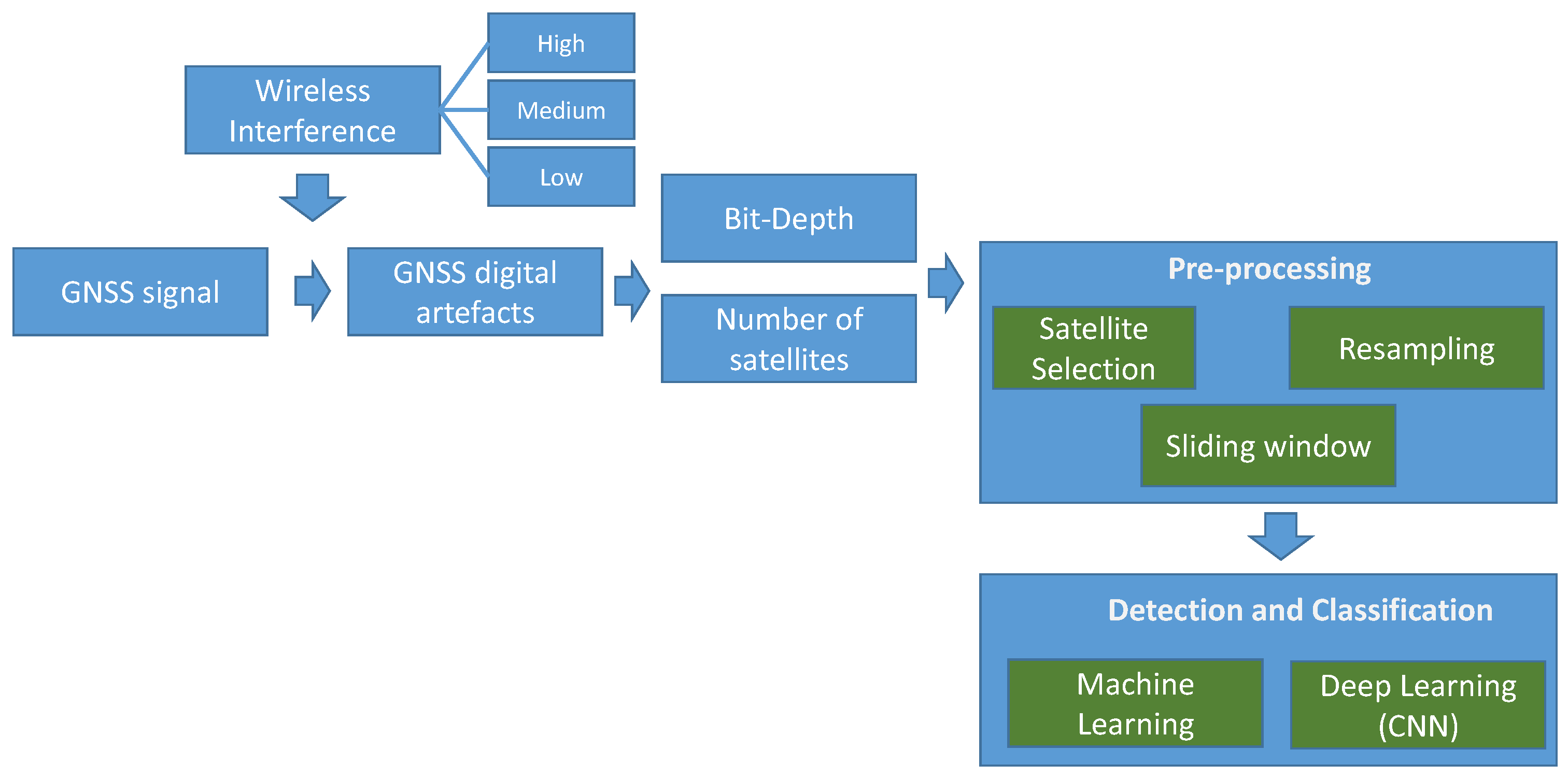
3.1. Main Flow and Procedures of the Proposed Approach

The overall methodology is pictorially described in Figure 1. On each of the C / N 0 time series generated by the GNSS receiver for each satellite in the constellation, an analysis of the quality of the data is performed. On the overall set of 47 satellites (24 GPS and 23 Galileo satellites), roughly half were in conditions of visibility and not all of them provided significant information for the detection of the interference because the GNSS signal did not have enough strength for the whole measurement duration. The consequence is that the generated C / N 0 would not have enough C / N 0 points for further processing or its level would be below an acceptable threshold. For this reason, a pre-processing step is performed, where only the satellites with a significant mean value are considered. The application of a threshold-based approach for filtering the appropriate satellites may not be suitable in this context for the following reasons: (1) It is difficult to set a specific threshold level and the consequent steps in the methodology could be biased by a wrong threshold value. On the other hand, an optimization of the threshold would require the repeated execution of the entire set of procedures described in this methodology, which would be quite time consuming. (2) Due to the presence of interference, the C / N 0 series are different for each interference condition or level of attenuation or bit-depth in the data set. As a consequence, a filtering step with the threshold may create unbalanced data sets across the different conditions, which may complicate the application of ML/DL more. This approach is based on a sorting of the average C / N 0 values for each satellite time series where only the first 8 satellites are considered. The number 8 was chosen as a trade-off between having enough satellites for the application of ML/DL and the need to have C / N 0 time series with a significant level of quality ( C / N 0 over 36 dB-Hz). As a consequence, this first pre-processing step for the GNSS satellite selection is data driven and it does not require hyper-parameters.
The subsequent step is to apply a sliding window with an overlapping factor on the C / N 0 time series for each of the considered 8 satellites. While both the overlapping factor and the length of the sliding window could be considered hyper-parameters in a generic time series analysis, their values can be defined in this specific context because the GNSS receiver will process the GNSS signal in a limited number of samples and a small value of overlapping factor should be used. The length of the sliding window should also be long enough to support the estimate of statistical features in the ML approach and to support the application of the CNN in the DL approach. In addition, the overlapping factor should be small enough to produce a significant number of samples in the C / N 0 time series with a length of 17,448 samples. Based on these considerations, a value of 4 was chosen for the overlapping factor and a value of 32 for the sliding window size to produce a data set of 433 samples for each satellite. In the next phase, two different branches of the methodology are adopted. For the ML approach, a set of features were applied to each sliding window to create a feature space for each satellite. The feature spaces were concatenated on the 8 satellites to create the final feature space on which the shallow Machine Learning algorithms described in Section 3.2 are applied. For the DL approach, the segments based on the sliding window length were used as input to the CNN. However, the size of the data set (433 samples) may be too small for the application of the CNN. To address this aspect, a simple data augmentation based on the application of Additive White Gaussian Noise (AWGN) with values ±1 dB was used to increase it to three times the size of the original data set. See [15,16] for a discussion on the advantages of data augmentation for CNNs. Finally, both the ML and DL algorithms were applied to each of the 15 interference conditions (3 levels of attenuation × 5 levels of bit-depth) for the different tasks of interference detection and interference identification (see Section 4 for a description of the interferences). The detection task is a binary classification problem (identify samples with the presence of interference from the ones with the absence of interference), while the identification of the type of interference is a multi-class (the three classes are Wide, Gaussian, and Narrow interference) problem.

3.2. Feature-Based Approach with Machine Learning Algorithms

A feature-based approach with three different shallow ML algorithms was used as a comparison to the CNN. The features are applied to the windows of the C / N 0 time series and they are selected due to the specific characteristics of this context: the presence or absence of interference will, respectively, decrease or increase the C / N 0 values. Features that provide an estimate of the values or a change in values are preferred. Ultimately, the nine features listed here were selected: minimum value, maximum value, Root Mean Square (RMS), skewness, kurtosis, standard deviation, and quantile with proportion 0.7, 0.8, and 0.9.
Three different classifiers were used in this study: the Decision Tree (DT) algorithm, the Random Forest (RaF) algorithm, and the Extremely Randomized Tree (ERT) algorithm. The ERT algorithm, which is an evolution of tree-based ensemble methods, is described by the authors of [17]. The DT algorithm is based on the MATLAB 2023a implementation using the templateTree and fitecoc functions configured with the automatic hyper-parameters optimization. The RaF algorithm is based on the MATLAB 2023a implementation using the templateTree and fitcensemble functions with the Adaptive Boosting algorithm (i.e., AdaBoost) and the automatic hyper-parameters optimization.

3.3. CNN Architecture and Hyper-Parameters

A two-layer CNN with multi-head attention and the Adaptive moment estimation (Adam) solver is used to implement the DL branch of the proposed approach.
A visual representation of the CNN architecture is shown in Figure 2, while the specific values of the CNN parameters are shown in Table 1.
These values were identified as optimal for the classification problem. The relatively low value for the number of epochs was set to 30 to mitigate the risk of overfitting. For the same reason, a 3-fold approach was used and the CNN classification was repeated 10 times (for a total of 30 executions of the ML algorithm). The resulting metrics were averaged. The cross-entropy loss was used as loss function.

3.4. Metrics of Evaluation

The evaluation metrics used in this study are accuracy, recall, and precision.
The accuracy is defined as
A c c u r a c y = T P + T N T P + T N + F P + F N .
where TP and TN are the numbers of True Positives and Negatives, respectively, FP and FN are the numbers of False Positives and Negatives, respectively.
The precision is defined by the following equation:
P r e c i s i o n = T P T P + F P .
The recall is defined by the following equation:
R e c a l l = T P T P + F N .
F1 score is defined by the following equation:
F 1 s c o r e = 2 × P r e c i s i o n × R e c a l l P r e c i s i o n + R e c a l l .
Confusion matrices are also used a classification metrics. This paper adopts the convention that column of the matrix represents the instances in an actual class while each row represents the instances in a predicted class.

3.5. Computing Platform

The computing platform used to conduct the experimental evaluation is a workstation equipped with an Intel I9-990KF Central Processing Unit (CPU) (Intel is based in Santa Clara, CA, USA) with a clock speed of 3.6 GHz, 32 Gbytes of Random Access Memory (RAM), and the Graphic Processing Unit (GPU) NVIDIA RTX4000. NVIDIA is based in Santa Clara, CA, USA. MATLAB R2023a from MathWorks was used to perform the scientific computations with the Signal Processing toolbox and the Machine Learning and Deep Learning toolbox. MathWorks is based in Natick, MA, USA.

4. Data Set Generation and Processing
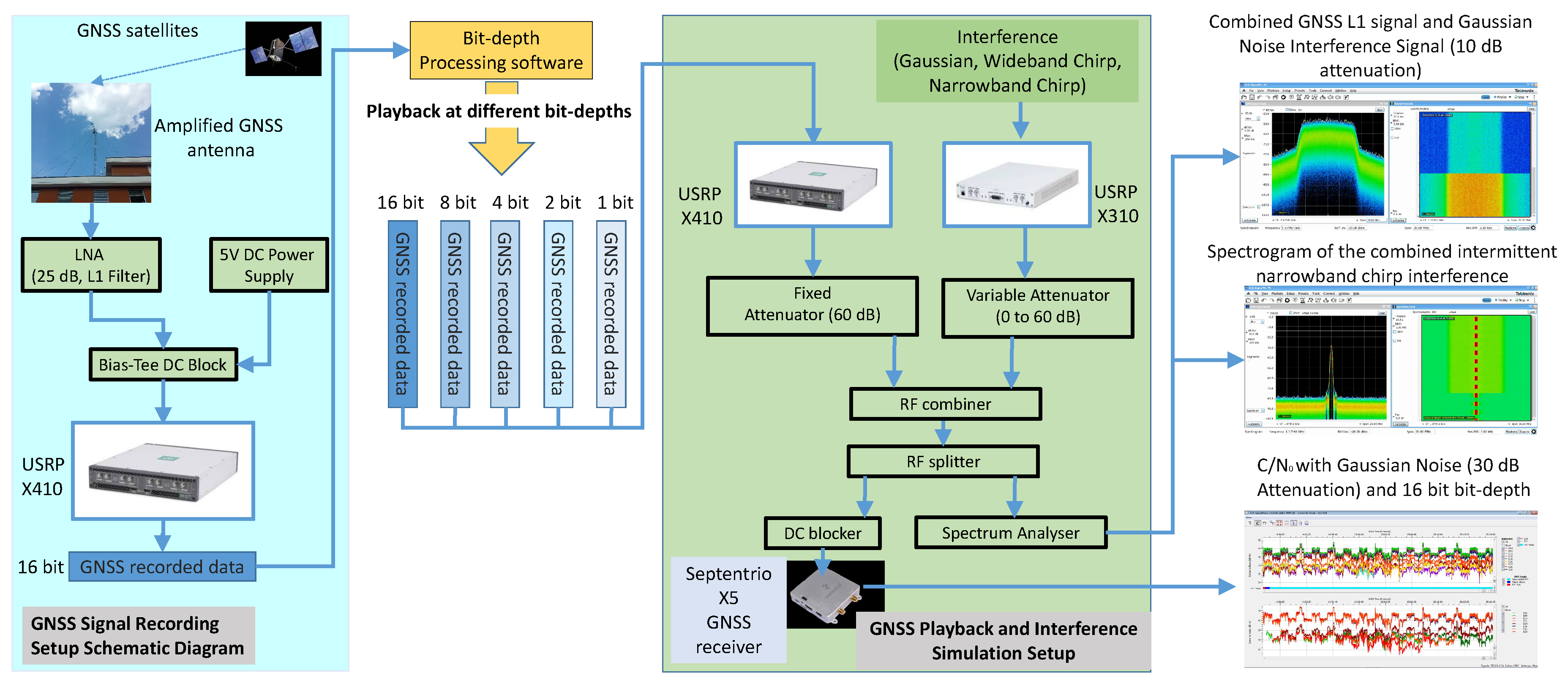
This section describes the data set used to evaluate the proposed approach with a breakdown in Section 4.1 for the description of the test bed and equipment used to generate the data set, Section 4.2 for the GNSS signal model and the description of the types of interference, Section 4.3 for the playback configuration with different bit-depths, Section 4.4 for the GNSS receiver configuration, and Section 4.5 for the description of the data set structure and format.

4.1. Test Bed Setup

The test bed is composed of the following equipment and the overall setup of the components. The transformation of the GNSS signal in space to the GNSS receiver’s artifacts (i.e., C / N 0 ) values) is shown in Figure 3.
The system includes the following:
  • Hardware component USRP X410, which is the primary GNSS recording and playback system, configured with a custom LabVIEW-based application. Labview is a graphical system design and development platform produced and distributed by National Instruments. National Instruments is based in Austin, TX, USA.
  • Hardware component X310 (interferent signal generation) is utilized with GNU’s Not Unix (GNU) Radio on Ubuntu to generate diverse interferent signals, including Gaussian noise, narrowband chirp, and wideband chirp.
  • Variable attenuator precisely controls the power level of the interferer.
  • Software component Windows Platform LabVIEW-based application with standard LabVIEW driver based on USRP Hardware Driver (UHD) was chosen for its compatibility with the X410 Universal Software Radio Peripheral (USRP) and for the implementation of bit-depth reduction.
  • Software component Ubuntu Environment GNU Radio is used for generating the interference signals.
The Software-Defined Radio (SDR) platforms are key components of the test bed and they are briefly described here. As described above, two SDR platforms are used in the test bed: the NI-Ettus X410 USRP and X310. The X410 is a new high-performance platform that builds on the success of the previous generation of USRPs, such as the N210, N310, X300, X310, and NI-2944r. This model is implemented with a new FPGA-based architecture that provides up to 400 MHz of instantaneous bandwidth per channel, which is twice that of the previous generation of USRPs. In addition, the X410 communication element includes two QSFP28 ports, which are able to support data rates of up to 4 × 25 Gbps, which provides significant support for high-speed data transfer and communication. The X410 analog front-end includes the ZBX two-channel superheterodyne transceiver, which supports frequencies ranging from 1 MHz to 8 GHz. It is an improvement in comparison to its older USRP counterparts thanks to the the implementation of a double intermediate frequency (IF) architecture, encompassing both intermediate (IF1) and baseband (IF2) stages. This design mitigates the DC offset problem associated with older zero-IF devices. In other words, unlike the X310’s zero-IF approach, the X410 eliminates the potential issue of an undesired carrier component acting as an unintentional GNSS jammer. This, combined with its improved sensitivity and dynamic range, makes the X410 ideal for faithful recording and playback of GNSS signals, ensuring the integrity of our study. In this setup, the X410 is used for the collection of the GNSS signal with 16 bit and the consequent playback with different bit-depths as described in Section 4.3.
The X310 is a high-performance, scalable SDR, which combines two extended-bandwidth daughterboard slots covering DC 6 GHz with up to 160 MHz of baseband bandwidth. In this study, only one of the ports is used. The X310 is used to generate the interference signals described in Section 4.2 using its zero-IF architecture. The X310 output gain is kept constant throughout the experiment to ensure that the interfering signal always maintains a consistent power level not greater than −50 dB over the entire 10 MHz bandwidth.

4.2. GNSS Signal Model and Types of Interference

At the GNSS receiver front-end, the GNSS signal from the different satellites is down-converted to Intermediate Frequency (IF), sampled into a digital sequence, and finally sent to the acquisition and tracking blocks. The received signal is expressed as follows:
r ( t ) = i = 1 N s ( i ) + w ( t ) + q ( t )
where N is the overall number of satellites considered in this study, i indicates the ith satellite signal, w(t) is the zero-mean white Gaussian noise with variance σ 2 , and q(t) is the interference signal. The desired GNSS signal from the i t h satellite is given by
s i ( t ) = P i D i ( t τ i ) · C i ( t τ i ) · e ( j ( 2 π ( f I F f d , i t + ϕ i )
where i denotes the index of in-view satellites; P i is the received power; C i ( ) and D i ( ) are the ±1-valued pseudorandom spreading code and navigation message, respectively; and τ i , f I F , f d , i , and ϕ i are the code delay introduced by the channel, IF used by the receiver front-end, carrier Doppler frequency, and carrier phase, respectively. Three type of interferences are considered. Wideband and narrowband chirp interferences are represented by
q ( t ) = P j e j 2 π f i n i t t + π f m a x f m i n T s w p t 2 + ϕ j
where for wideband f m a x and f m i n are 1.57542 GHz (i.e., f i n i t ) ± 5 MHz and T s w p is 5 μs. For narrowband interference, f m a x and f m i n are 1.57542 GHz (i.e., f i n i t ) ± 20 KHz and T s w p is 1 ms.
The Gaussian band interference (random noise characterized by its Gaussian normal distribution) is represented by
q ( t ) = P j i a i g ( t i T a ) c o s ( 2 π f j t + ϕ j )
where g(t) represents the impulse response of shaping filter, a i is the pseudorandom code that takes the value −1, +1, and T a is the code duration time.
These types of interference have been used because they are adopted in [3] and for the following reasons. Gaussian noise is introduced to simulate the background noise present in real-world environments, such as electromagnetic interference from natural and man-made sources. Wideband chirps mimic interference sources such as radar systems or broadband communication signals. Narrowband chirp interference poses a unique threat to GNSS receivers by potentially disrupting the timing synchronization process.

4.3. GNSS Signal and Playback with Specific Bit-Depth

The data set is created using recorded GNSS signals from an amplified roof antenna (to ensure adequate reception strength) installed in the JRC premises. Then, real-world signal and not simulated signals are used for the study. A 25 dB Low Noise Amplifier (LNA), which includes a GPS L1 band RF filter as well, is introduced to further bolster the signal level, mitigating potential noise issues. We consider the GPS L1 band even if the data set includes Galileo E1. To power this external LNA, a bias-tee and a 5V Direct Current (DC) power supply are incorporated, ensuring its functionality while simultaneously DC blocking the RF to the output. This step prevents any unwanted DC components from reaching the subsequent component in the signal processing chain (e.g., X410’s RF input), maintaining signal integrity. In the X410 SDR, the RF analog signal undergoes conversion to the digital domain with a sampling rate of 10 MSamples/Sec using a bandwidth of 10 MHz and bit-depth of 16 bits. This sampling rate and bit-depth provide sufficient resolution to capture the relevant information within the chosen GPS L1 and Galileo E1 bands and keep the recorded files small enough. See [18,19] for an analysis of the bit-depth impact in GNSS recording and playback. The center frequency is set to 1.57542 GHz, encompassing both the L1 and E1 bands and the maximum gain of 59 dB was used in the LNA of the X410 (to ensure adequate signal strength for optimal recording). An extended recording duration of 30 min was employed. This timeframe allows for the observation of signal variations arising from environmental fluctuations, satellite movements, and potential interference events.
The next step is to create a representation of the GNSS signal for playback with different bit-depths, which is one of the main objectives of the study presented in this paper. This was achieved with a custom LabVIEW application designed specifically for this purpose to synthesize signal files at various bit-depths: 8, 4, 2, and 1 bit-depths starting from the original 30 min file recorded at 16 bits. The algorithm implemented with LabVIEW discards less significant bits to achieve the desired bit-depth. For example, transitioning from 16 to 8 bits involves eliminating the 8 least significant bits while retaining the most significant 8 bits in the output file. The algorithm was designed to preserve negative numbers with two’s complement: the bit reduction may impact negative values, essential for In-phase and Quadrature component (IQ) signals. By using this representation, discarding the Least Significant Bits (LSBs) preserves the sign bit and, consequently, the negative values embedded within the signal. This ensures accurate representation of both positive and negative components, which is crucial for faithful signal reconstruction. On the other hand, discarding LSBs effectively reduces the signal’s dynamic range. To maintain accurate representation after this reduction, the original signal must possess sufficient power in its Most Significant Bits (MSBs), which is the reason why the maximum gain of 59 dB was used.
Some background information on the USRP digital representation and the two’s complement is provided here because it is a core part of the bit-depth aspect of this study. USRPs handle numbers in integer binary format, using 16-bit sequences of 0 s and 1 s. An I16 integer (signed 16-bit integer) can represent values from −32,768 to 32,767. Each bit has a specific weight based on its position, starting with 2 0 for the least significant bit (LSB) and increasing by a power of 2 for each bit to the left. The positive numbers are directly represented by their binary equivalent (e.g., the decimal number 10 in 16-bit binary is 0000 0000 0000 1010 with 0 × 2 0 + 1 × 2 1 + 0 × 2 2 + 1 × 2 3 + 0 × 2 4 + 0 × 2 5 + 0 × 2 6 + 0 × 2 7 + 0 × 2 8 + 0 × 2 9 + 0 × 2 10 + 0 × 2 11 + 0 × 2 12 + 0 × 2 13 + 0 × 2 14 + 0 × 2 15 = 10 dec). The negative numbers are represented with the two’s complement by taking the absolute value of the number (e.g., 10), converting it to 16-bit binary (e.g., 0000 0000 0000 1010), inverting each bit (e.g, 1111 1111 1111 0101), and adding 1 to generate the final binary representation (e.g., 1111 1111 1111 0110). The key point is that the Most Significant Bit (MSB) of a two’s complement number determines its sign: 0 for positive, 1 for negative. Therefore, discarding less significant bits in two’s complement representation preserves the sign bit, maintaining both positive and negative values. In the algorithm implemented in this study, to achieve bit-depths lower than 16 (e.g., 4), the discarding of the Least Significant Bit (LSB)s does not impact the sign information. If we take, for example, the decimal number −15,234, represented in binary as 1100 0100 0111 1110, discarding the four LSBs generates 1100 0100 0111. During playback, the digital content is converted back to I16 by treating the discarded bits as zeros: 1100 0100 0111 becomes 1100 0100 0111 0000. This results in the decimal value −15,248, which is very close to the original one, as expected. Although the precision is reduced, the sign bit (1) is preserved, reflecting the negative nature of the original value. In general, the error introduced by discarding the four LSBs ranges from 0000 to 1111 (15 dB), causing a minor loss in precision.
To enhance the realism of the interference simulation, the continuous interference signals generated in the L1 band were transformed into burst transmissions. This intermittent behavior, where the jammer alternates between one-minute ‘on’ and ‘off’ periods, better reflects the characteristics of certain real-world interference sources. This intermittent effect was created on the continuous data stream generated by the chirp signal process (involving the Signal Source and Voltage-Controlled Oscillator (VCO) blocks) by segmentation using the stream to tag the stream block (see Figure 4). The burst shaper block was employed to selectively manipulate the tagged packets. This block was configured to create alternating one-minute intervals where the interference signal is passed through (‘on’ state) and suppressed (‘off’ state). These intermittent values were also used to define the label information.
Each interference condition is generated using a specific power level of the interferer, which may change due to the type of interference in the attempt to make the impact visible in the C / N 0 equivalent (e.g., a wideband chirp interferer has a larger impact than a narrowband chirp interferer at the same level of dB). The power levels of the interference are defined by setting the attenuation (using the variable attenuator shown in Figure 3) to the values presented in Table 2 and represented in the rest of this paper as L I = L (low), L I = M (medium), and L I = H (high),

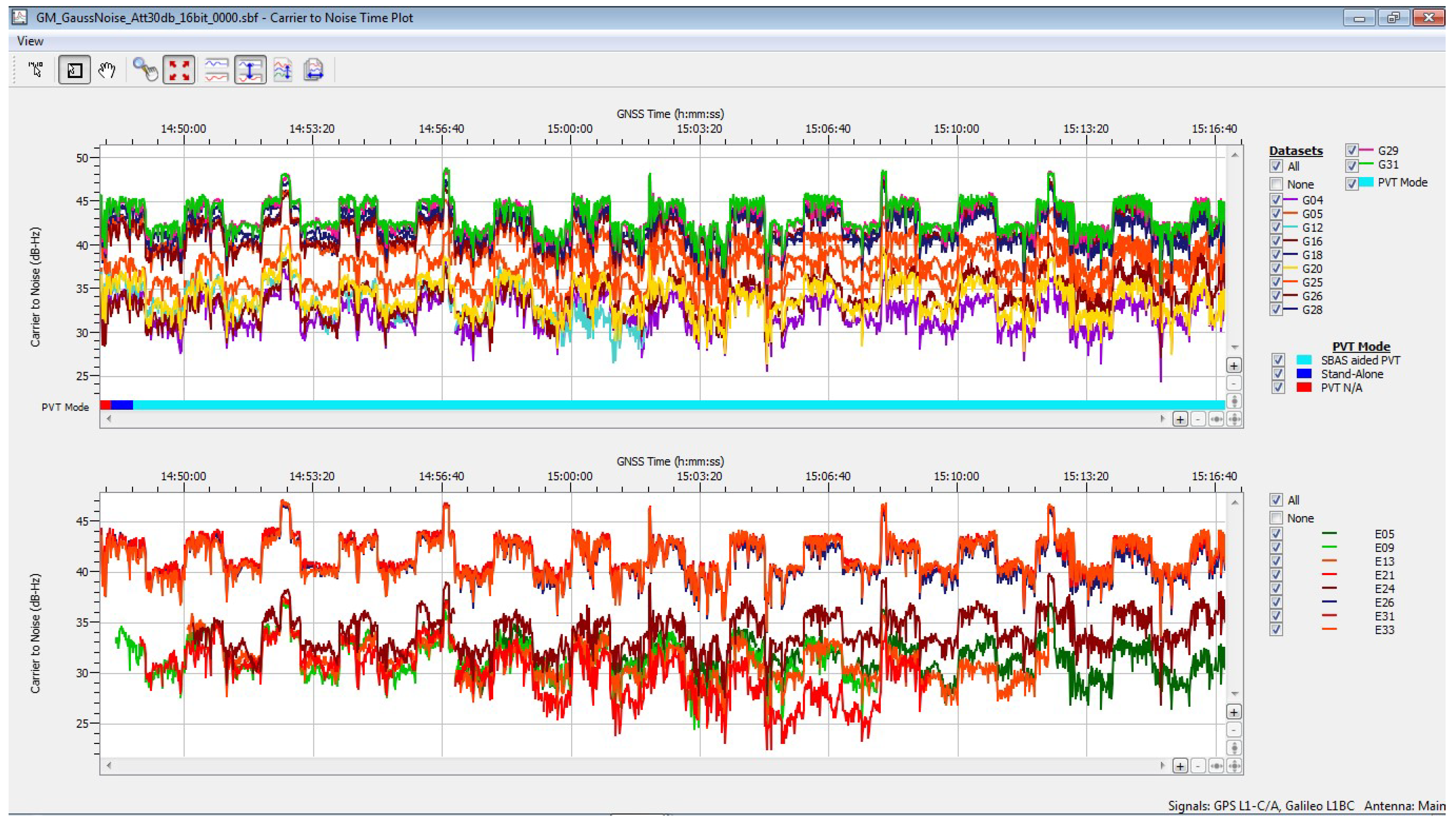
4.4. GNSS Receiver Configuration and Generated Digital Artifacts

The experiment utilizes a Septentrio Mosaic X5 GNSS receiver for real-time data acquisition and logging, which generates the C / N 0 time series per satellite at a frequency of 1 Hz. This metric measures the signal strength of each tracked satellite relative to the background noise level. C / N 0 indicates a strong capability to accurately track and decode satellite data.
An example of the impact of the interference on the GNSS C / N 0 s artifacts is shown in Figure 5.
The presence of spikes can be noted in Figure 5. These spikes are due to the Automatic Gain Control (AGC) algorithm employed in the Septentrio Mosaic X5 GNSS receiver. Septentrio is based in Leuven, Belgium. This algorithm dynamically adjusts the gain level to maintain a consistent signal strength, leading to temporary increases when the signal weakens corresponding to the observed C / N 0 spikes. Other mechanisms implemented in the GNSS receiver, which may influence the C / N 0 generation, are the carrier notch filters (which attenuate narrowband interference around the GNSS carrier frequency), integration time (affects smoothing of C / N 0 plots), and GNSS selection (allows focusing on specific constellations). We use the default settings for the GNSS receiver. The selected timing source is the GPS constellation.

4.5. Data Set Structure and Format

The generated data set is composed of the C / N 0 data generated by the Septentrio receiver for almost 30 min of signal playback at a rate of 1 Hz. Thus, a time series composed of 1748 C / N 0 values was generated for each of the considered satellites (32) for each level of bit-depth (i.e., five bit-depths), three power levels (e.g., L I = M ), and four types of interference scenarios (i.e., three types of interference and the absence of interference). Taking into consideration that the chosen step is 4 and the window size is 16 C / N 0 value, 433 window samples were generated on which the feature and the CNN were applied. As mentioned before, an analysis of the C / N 0 samples from the different satellites showed that not all the satellites are suitable for the analysis because of periods of signal unavailability, which led to missing samples or samples degraded to low values of C / N 0 . The rule was to consider only satellite, where the number of generated values of C / N 0 was not less than 90% of the 1748 samples and value of the C / N 0 was higher than 34 dB-Hz for two-thirds of the data samples. This was an empirical approach, which can be further refined in future developments, and it is based on the consideration that there should be enough valid samples (i.e., C / N 0 values corresponding to the signals of GNSS satellites with LOS propagation conditions of satellite fix) to support the ML classification. The threshold of 90% was inspired by similar studies where such threshold values were used on the C / N 0 to distinguish between propagation conditions [20]. The result of this filtering step identified only eight satellites that were suitable for the subsequent phases.
Even these eight satellites could have significant variability in the number of samples, and a resampling step was performed with the MATLAB interp1 function and two different algorithms: linear interpolation and nearest neighbor interpolation. These algorithms were chosen on the basis of the characteristics of the C / N 0 time series with steep transients, which prompted the authors to discard other algorithms (i.e., cubic spline). The result from the two interpolation algorithms were basically equivalent and the linear interpolation was chosen for its computational speed.
Because the number of samples for each type of interference and bit-depth could be limited to train the CNN algorithm, a simple augmentation step was implemented to increase the number of samples. Two other sets of 433 samples were generated with AWGN of 1 dB higher and lower than the measured SNR of the original C / N 0 time series. Considering the case of interference classification, this resulted in a DL problem with 1299 samples × 3 types of interference to have 3897 samples in total as input to the CNN. In addition, to provide an input wide enough for the CNN classifier, the C / N 0 time series was resampled by a factor of 2 after the interpolation (i.e., the window given in input to the CNN has length 32).

5. Results and Discussion

This section presents the results of the application of the proposed approach described in Section 3 on the data set described in Section 4. This section is structured as follows: Section 5.1 focuses on the detection of interference, which is implemented as a binary classification problem. Section 5.2 focuses on the identification (i.e., multi-class classification) of the different types of interference considered in this study: wideband, Gaussian, and narrowband interference to the GNSS signal. Finally, Section 5.3 discusses the limitations of the proposed approach.

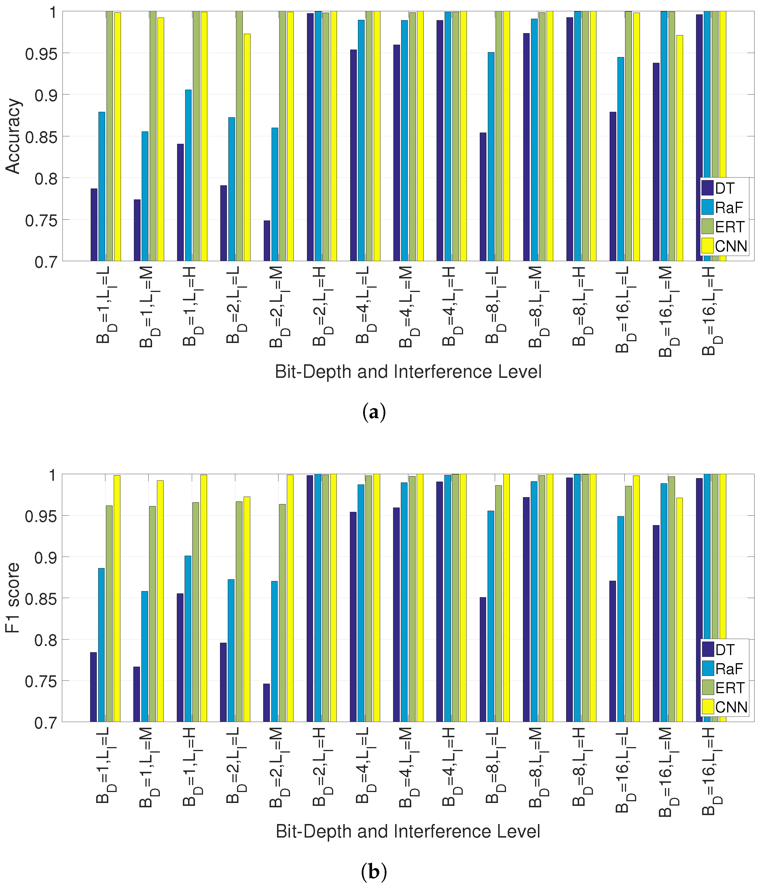
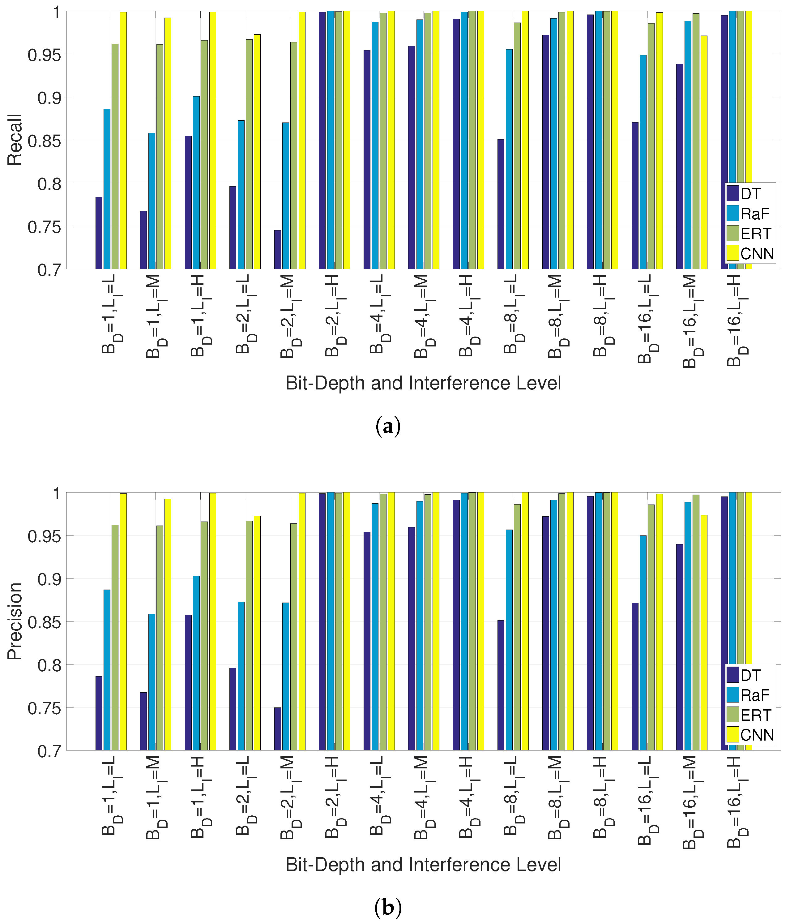
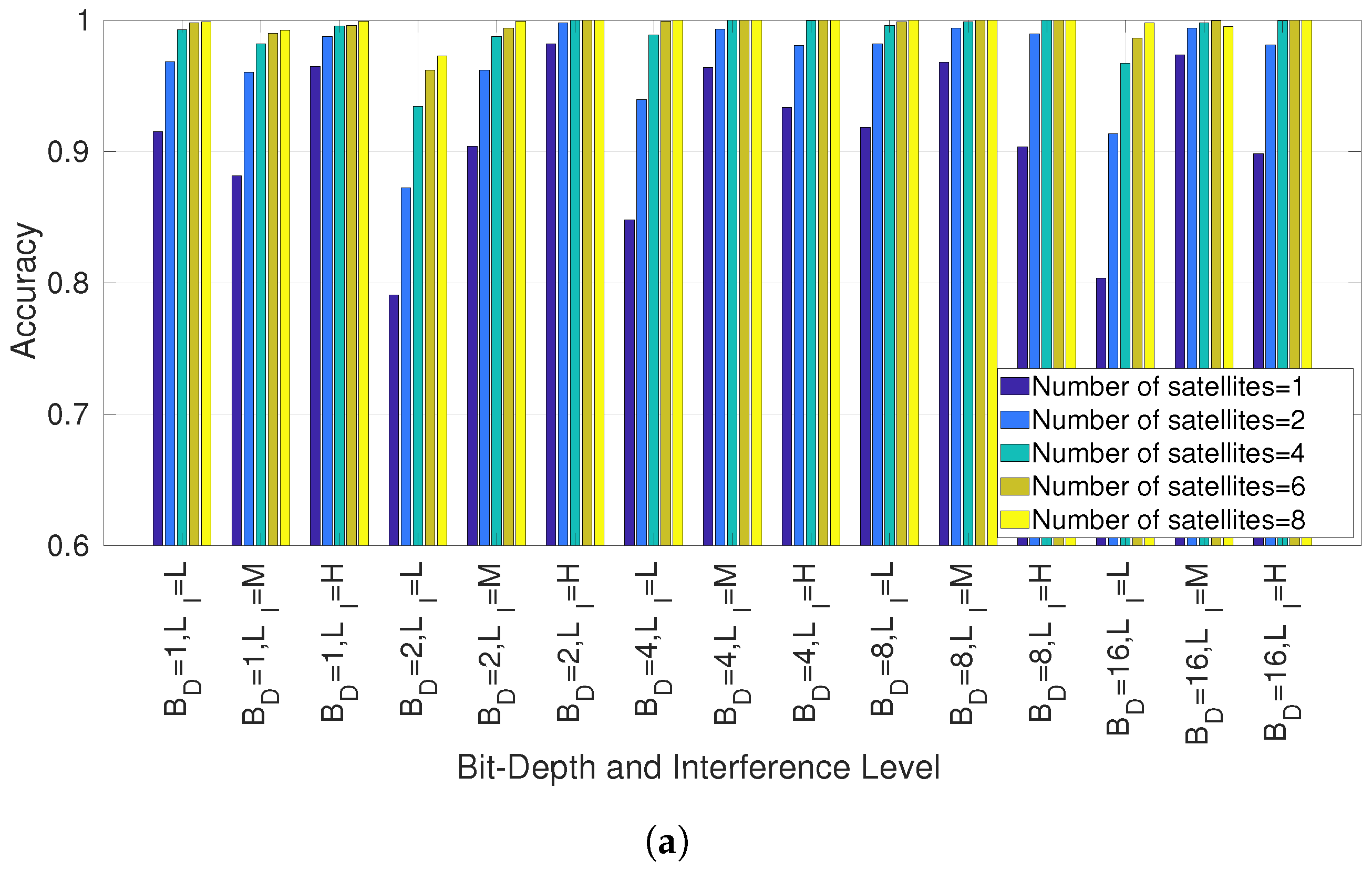
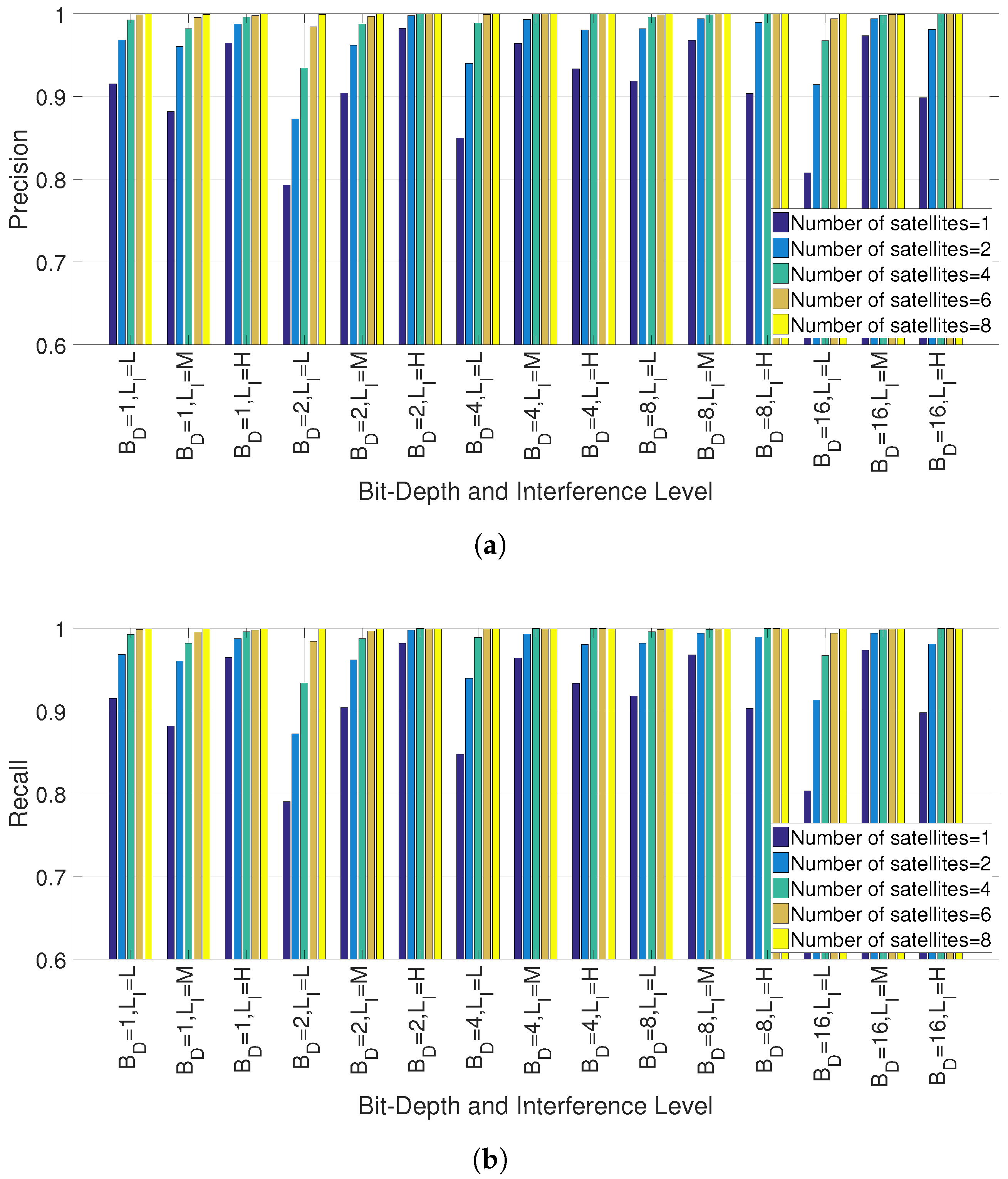
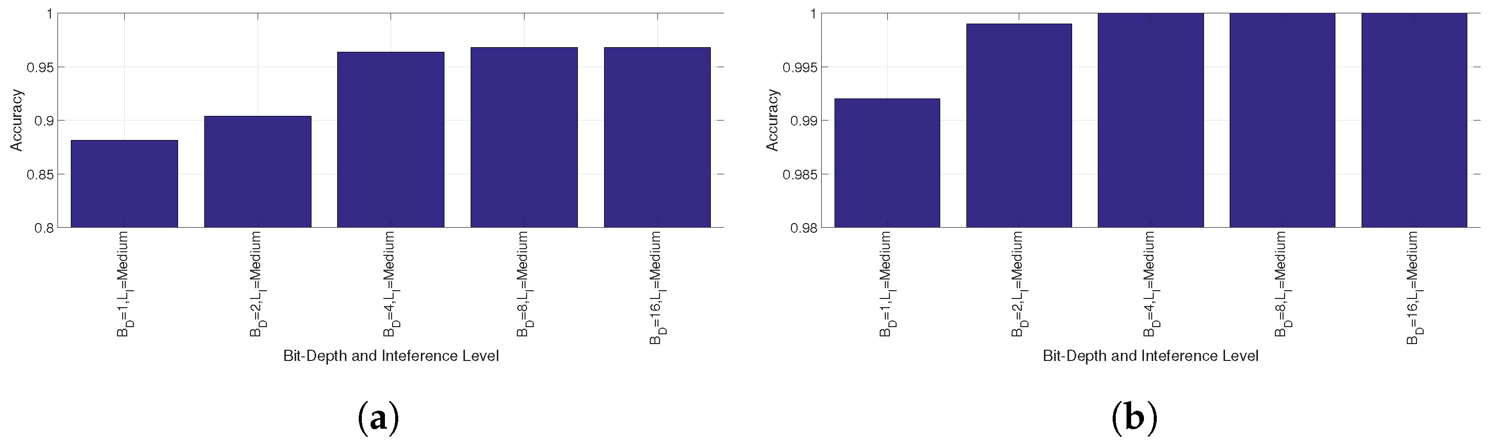
5.1. Detection of Interference

Figure 6 and the related sub-figures show the detection results using the feature-based approach for the metric of accuracy, Figure 7 and sub-figures show the precision, and Figure 8 and sub-figures show the recall for different levels of attenuation. In particular, Figure 6a, Figure 6b, and Figure 6c show, respectively, the detection accuracy for low, medium, and high levels of interference for the three types of interference and different levels of bit-depth (called B D in the rest of this section) as shown in the legend. In a similar way, Figure 7a–c show the precision values and Figure 8a–c show the recall values. Regarding B D , the results are generally consistent across the metrics and the types of interference: a higher value of B D (e.g., 16 bits in comparison to 2 bits) provides a higher value of the metric (e.g., accuracy). The differences are more significant for low levels of interference, where the detection algorithm has more difficulty in detecting the interference. This is to be expected because a high value of B D provides richer and more discriminating information to the detection algorithm, which supports a better detection of the interference. However, the figures seem to indicate that B D = 16 bits are not needed to achieve the optimal results. Values of 8 bits also provide a detection performance comparable to 16 bits. These results can be used to reduce the amount of data needed to perform the detection of interference.
The higher the level of interference, the higher the value of the performance (e.g., higher accuracy). This is also to be expected because the higher the level is the more significant the impact on the GNSS signal, which translates to a higher variation in the C / N 0 time series.
The results for the different types of interferences are somewhat varied and they depend on the level of interference. This may also be related to the different interference power levels defined in Table 2. Narrow interference can be detected more easily than Wide and Gaussian interference for low levels of interference, but the Gaussian interference is detected with higher accuracy with the higher power level of interference.
Similar results are achieved using the CNN algorithm. To conserve space, only the accuracy results are shown because the precision and recall graphs present similar results. The comparison of Figure 9 with Figure 6a–c shows that the CNN is able to obtain a superior detection performance at the cost of a higher computing complexity. In particular, for higher values of B D , the CNN algorithm can obtain perfect detection (i.e., 100 % ) or near perfection. For the value of B D = 1 , even the CNN algorithm has a significant number of misclassification errors because the lower bit-depth degrades significantly discriminating features, which can be used by the CNN to detect the interference. As expected (and coherently with the feature-based approach), a low level of interference causes a lower detection accuracy, especially for the Wide and Narrow types of interference, while the CNN reaches almost perfect detection for values of B D higher or equal than 4.

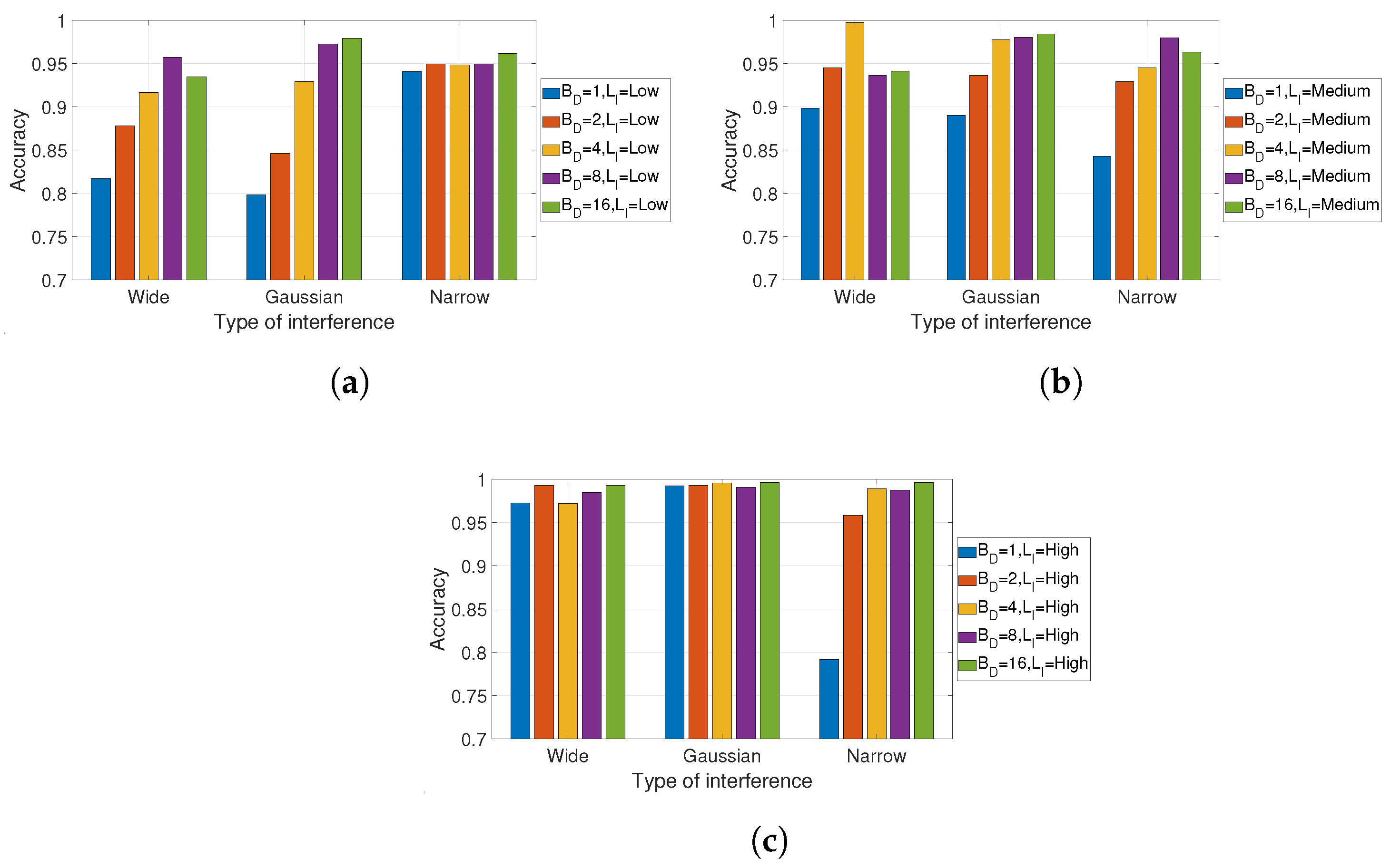
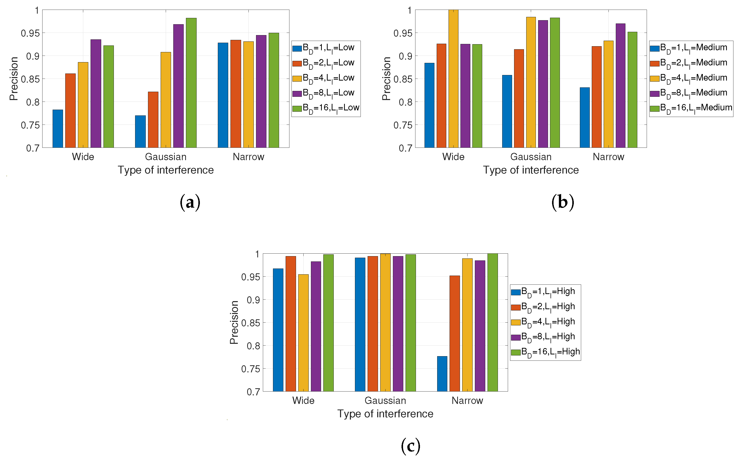
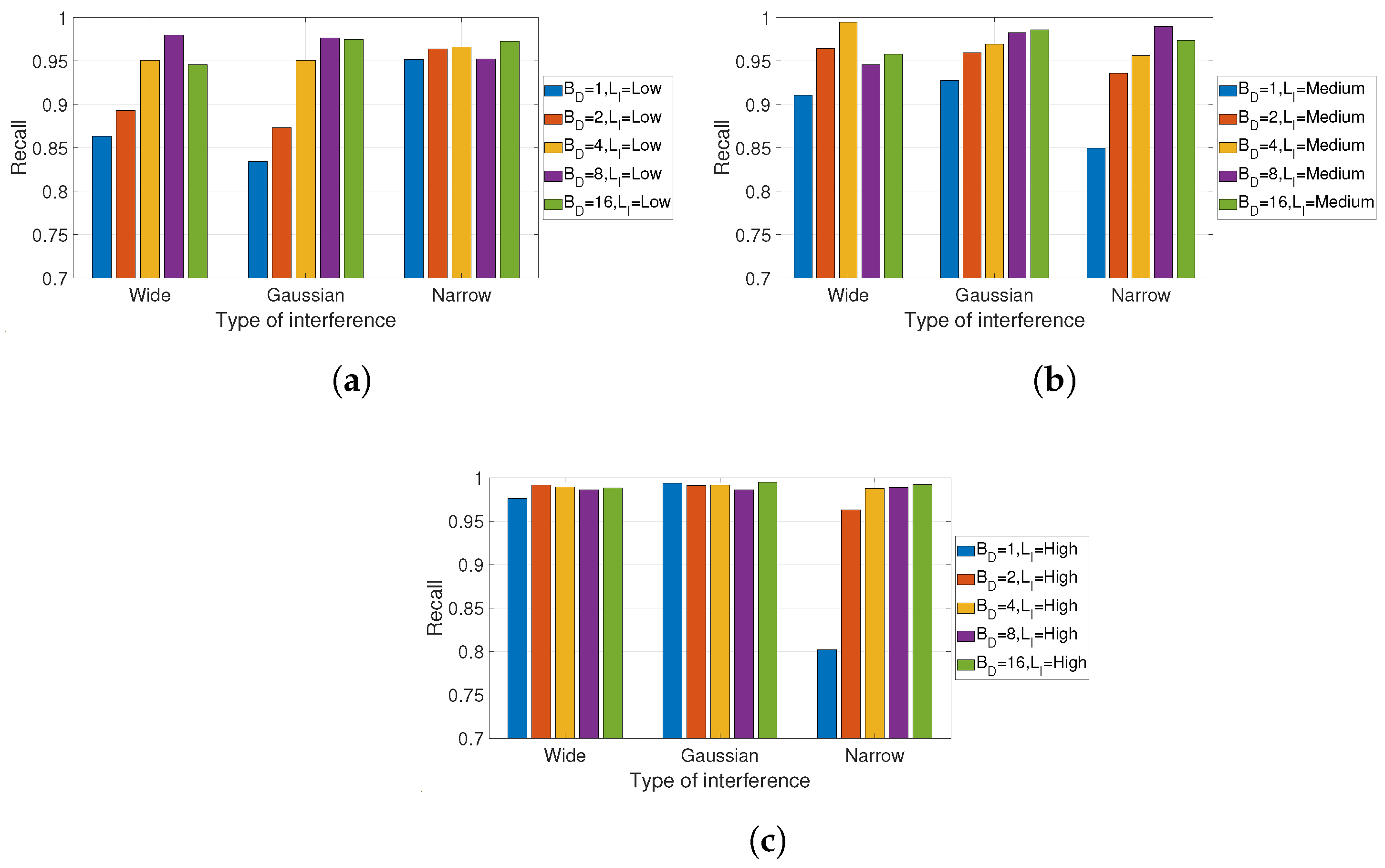
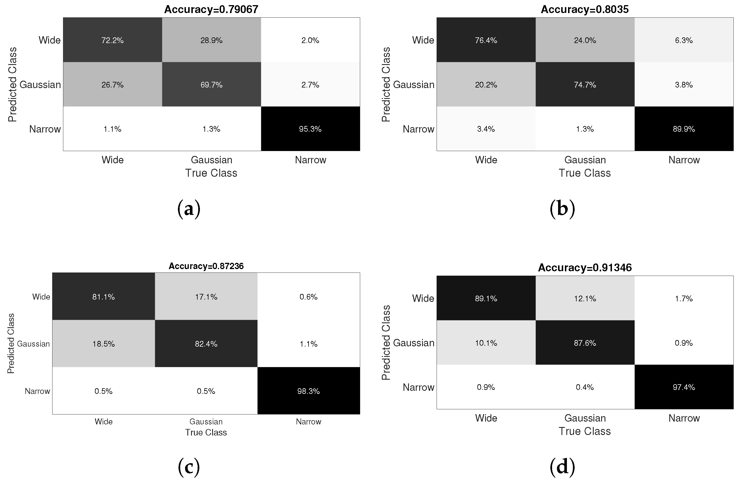
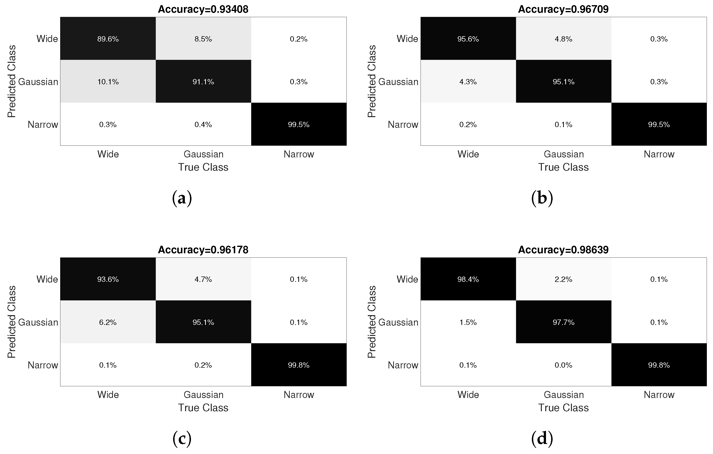
5.2. Classification of Interference

Figure 10 and related sub-figures show the comparison of the accuracy and F1-score using the CNN and the shallow ML algorithms using the feature-based approach. These results are obtained using the C / N 0 data obtained from all eight GNSS satellites obtained after the filtering step described in Section 4.5.
In particular, Figure 10a, Figure 10b, Figure 11a, and Figure 11b present, respectively, the accuracy, F1 score, precision, and recall for different levels of bit-depth and interference level (x-axis). The figures show that the four metrics are generally coherent among themselves. The CNN algorithm generally demonstrates a superior performance to the shallow ML algorithms with the exception of the ERT, because the ERT equals CNN for some cases or it is even better with B D = 16 and L I = M . Considering the ERT has a significantly lower computing complexity than the CNN, ERT could be the preferred choice for computing efficient deployments of this approach. ERT mostly outperforms RaF and DT, which justifies the proposal of ERT in this study. It can be noted that for values of B D = 1 and B D = 2 , the classification performance drops significantly for the RaF and DT algorithms, especially at a low level of the interference power L I = L . This is not surprising because the classifiers have difficulty in exploiting the discriminating content due to the limited available information (the reduction in the B D ) and the minor impact of interference signals with low levels of power because the variations of the C / N 0 are less prominent than for a high level of power. Even in the challenging conditions of low B D and L I , the performance of the CNN classifier is remarkable as it has almost 100% accuracy apart from the case of B D = 2 and L I = M , where it achieves 97% accuracy.
It is also important to evaluate the performance of the proposed approach for different numbers of satellites N S . Figure 12 and related sub-figures show the accuracy and F1 score while Figure 13 and related sub-figures present the precision and recall for different bit-depths and levels of interference using different numbers of satellites. These figures were obtained by averaging the results for repeated execution of the CNN algorithm for the potential combinations of satellites, respectively, in sets of one (8 executions), two (28 executions), four (70 executions), six (28 executions), and eight (1 executions). It can be seen that a larger number of satellites increases the classification accuracy across the different levels of B D and interference level. This is to be expected because a larger number of satellites can provide more (and more discriminating) information to the CNN classifier to identify the specific type of interference. On the other hand, for medium and high levels of interference, six satellites or even four satellites are enough to obtain an accuracy/precision and recall equal or similar to the one obtained with all eight satellites. Both Figure 12 and Figure 13 show that the proposed approach is able to obtain almost perfect accuracy/F1 score/precision/recall with B D higher than 4 and more than four satellites, which is evidence of the robustness of the proposed approach. The drop in classification performance is particularly significant between a number of satellites equal to one or two, especially for L I = L and L I = M . The analysis of these figures stresses the importance of the pre-processing phase to collect data from as many satellites as possible, because a lower number of satellites may significantly degrade the classification performance.
Figure 14 gives a more detailed view of the classification accuracy with L I = M for different values of the B D and for one satellite and all eight satellites. As shown in the previous figures, both the decrease in B D and N S lead to a decrease in classification accuracy.
To complement the previous results for accuracy, precision, and recall, we provide in the following Figure 15 and Figure 16 and related sub-figures the confusion matrices for different values of B D , L I , and N S . Predicted values are on the y-axis and True values are on the x-axis. The figures were generated using the CNN with L I = L , which is the most challenging for classification.
The figures show that the Wide and Gaussian types of interference are more difficult to classify in comparison to the Narrow type of interference. As expected, the number of FPs and FNs is lower in percentage (values outside the diagonal) when more satellites or a higher value of B D is used.

5.3. Discussion on the Limitations of the Proposed Approach

The main limitation of the approach presented in this paper is related to the data set and the filtering process where the data from the GNSS satellites is collected. Even if real-world signals were collected through a GNSS antenna located in a JRC premises, the position of the antenna was static and in a limited time frame of 30 min. On the basis of these data, an empirical filtering step was implemented to select a number of satellites, X, using a pre-defined threshold with the number of generated values of C / N 0 not less than 90% of the 1748 samples and values of the C / N 0 higher than 34 dB-Hz for two-thirds of the data samples. This filtering step indicated the X=8 satellites used in the analysis. In a dynamic context, where there could be significant variations in the propagation environment for the GNSS signal (e.g., a vehicle driving in a urban environment), the filtering step would benefit of a dynamic threshold setting where the number of satellites is adjusted according to the quality of C / N 0 generated by the GNSS receiver. It is also noted from the results presented in Section 5.2 that even with a number of satellites equal to four, the CNN and ERT classifiers manage to obtain a very high classification accuracy (i.e., 99% and higher). Then, the proposed approach may be robust even in a dynamic environment because even a limited set of GNSS satellites would be enough. Potential approaches to implement dynamic threshold, which have to be timely and computing-efficient, could be based on a optimization step linked to the threshold values (e.g., range of the percentage or C / N 0 threshold) where one of the classification metrics (e.g., accuracy) could be used as a cost function. Due to the need of timely execution, a shallow ML algorithm like the DT used in this paper could be selected for its computing efficiency, even if DT demonstrated a low performance in comparison to the CNN in Section 5.2. The creation of a dynamic data set with the related collection and generation of interference signals would be much more complex than the the current data set used in this paper, and this task is deferred to future developments as described in Section 6.
Another limitation of the proposed study is the use of only the C / N 0 data from the GNSS receiver. Even if they are related, other measures like Horizontal Dilution Of Precision (HDOP), Vertical Dilution Of Precision (VDOP), clock bias, the carrier phase, pseudorange metrics, and even the satellite elevation features could be used taking inspiration from the studies focused on GNSS LOS/NLOS classification [21,22]. This is also reserved to future developments.
Finally, even if the CNN classifier has demonstrated an excellent detection and classification performance, more recent and sophisticated neural networks models could be evaluated and adopted, like Transformers used for GNSS NLOS identification in [23]. On the other hand, especially in a dynamic environment, there is an important trade-off between computing efficiency and accuracy and it has to be seen if DL can be applicable or other neural network algorithms (e.g., feed-forward neural networks) could be more suitable.

6. Conclusions and Future Developments

This paper describes an approach to detect and classify different types of interferences on GNSS signals based on the application of ML/DL algorithms, where detection means the capability to reveal the presence of an interference condition in the processed GNSS signals, while classification refers to the capability to distinguish among different types of interference (i.e., wideband, Gaussian, and narrowband in this study). In particular, the impact of three main parameters was considered in the study: (1) the bit-depth at which the GNSS signal was played back before it was processed by the GNSS receiver, (2) the power level of the interference signal, and (3) the number of different GNSS satellites used to detect and classify the interference. This study used ML algorithms and neural networks/Deep Learning (DL) algorithms. The ML algorithms were a Decision Tree (DT), Random Forest (RaF), and Extremely Randomized Trees (ERT). The DL was a Convolutional Neural Network (CNN). The results show that the CNN is able to obtain almost perfect detection accuracy with high and medium levels of interference power and bit-depth equal or superior to 4 bits with the wideband and Gaussian interference and eight GNSS satellites. However, the accuracy drops with a bit-depth equal to 1 or 2, low interference level, and narrowband interference because the impact of the interference is less distinguishable in the GNSS receiver and because the bit-depth reduction removes discriminating information for the CNN classifier. Similar results are obtained for the interference classification task where perfect (100%) or almost perfect (greater than 99%) accuracy is generally obtained for bit-depth greater and including 4 bits and interference levels are medium or high, but it drops significantly for a low interference level and bit-depth of 1 or 2. The DT and RaF generally perform worst than the CNN. It is noted that the ERT algorithm often achieves a similar level of accuracy to the CNN with less computing resources, which could support its use in operational scenarios, which requires computational efficiency. The use of the number of satellites also has a significant impact. The classification performance degrades significantly when only the information from one or two satellites is used. The results show that the use of six satellites or eight satellites is quite similar, supporting the concept that with this specific data set, six satellites would be enough to distinguish with high accuracy the different types of interference. Then, there is a trade-off between the need to process more information from a larger number of satellites with the need for a high classification accuracy.
This paper has also discussed the limitations of the proposed approach. Even if real-data from GNSS constellations was used in the study in a significant amount of time, a dynamic environment where the signal quality from the different satellites changes frequently (e.g., a GNSS receiver mounted on a vehicle driving in an urban environment) may be challenging for the proposed approach where a fixed number of satellites is used. Then, an adaptive algorithm based on the quality of the received signal could be used to determine in a dynamic way the optimal number of satellites and address the trade-off mentioned above. The evaluation of the approach proposed in this paper to a vehicular dynamic context will be the objective of future extensions of this study.
Future developments could go in different directions. One direction would be to investigate the proposed approach on a dynamic environment (e.g., vehicle moving in an urban environment) where the propagation conditions change frequently. Then, new filtering steps should be investigated to determine the optimal thresholds in the data pre-processing phase. As suggested in the main body of this paper, a hybrid approach of shallow and deep ML algorithms could address the need for timely results and computing efficiency. Another direction may include the application of more sophisticated neural networks algorithms like a Transformer architecture for improved accuracy or feed-forward neural networks for higher computing efficiency. Taking in consideration the excellent performance of the ERT in this study, similar algorithms like Rotation Forest or Deep Forest could also be used. Finally, this study was mostly based on the use of Carrier-to-Noise Ratio information (e.g., C / N 0 ) but other relevant information provided by the GNSS receiver could also be used like carrier phase, pseudorange features, Horizontal Dilution Of Precision (HDOP) or Vertical Dilution Of Precision (VDOP).

Author Contributions

Conceptualization, G.B.; Methodology, G.B.; Software, G.B. and F.B.; Resources, G.B. and F.B.; Data Curation, G.B. and F.B.; Writing—Original Draft Preparation, G.B.; Writing—Review and Editing, G.B. and F.B. All authors have read and agreed to the published version of the manuscript.

Funding

This research received no external funding.

Institutional Review Board Statement

Not applicable.

Informed Consent Statement

Not applicable.

Data Availability Statement

The data presented in this study are available on request from the corresponding author. The data are not publicly available due to lack of approval of the data set publication by the JRC. The data set will be submitted to the internal JRC approval process for data publication after the acceptance of the publication.

Conflicts of Interest

Author Fausto Bonavitacola was employed by the company Piksel. The remaining authors declare that the research was conducted in the absence of any commercial or financial relationships that could be construed as a potential conflict of interest.

Abbreviations

The following abbreviations are used in this manuscript:
AdamAdaptive moment estimation
AGCAutomatic Gain Control
AWGNAdditive White Gaussian Noise
CNNConvolutional Neural Network
CNRCarrier-to-Noise Ratio
DCDirect Current
DLDeep Learning
ERTExtremely Randomized Tree
FPGAField-Programmable Gate Array
GPSGlobal Positioning System
GNSSGlobal Navigation Satellite System
HDOPHorizontal Dilution Of Precision
IFIntermediate Frequency
IQin-phase (I) and quadrature (Q)
JRCJoint Research Centre
LNALow Noise Amplifier
MLMachine Learning
RFIRadio Frequency Interference
SVMSupport Vector Machine
TFTime Frequency
UHDUSRP Hardware Driver
USRPUniversal Software Radio Peripheral
VCOVoltage-Controlled Oscillator
VDOPVertical Dilution Of Precision

References

  1. Siemuri, A.; Selvan, K.; Kuusniemi, H.; Valisuo, P.; Elmusrati, M.S. A systematic review of machine learning techniques for GNSS use cases. IEEE Trans. Aerosp. Electron. Syst. 2022, 58, 5043–5077. [Google Scholar] [CrossRef]
  2. Dimc, F.; Bažec, M.; Borio, D.; Gioia, C.; Baldini, G.; Basso, M. An Experimental Evaluation of Low-Cost GNSS Jamming Sensors. Navig. J. Inst. Navig. 2017, 64, 93–109. [Google Scholar] [CrossRef]
  3. Zhong, W.; Xiong, H.; Hua, Y.; Shah, D.H.; Liao, Z.; Xu, Y. TSFANet: Temporal-Spatial Feature Aggregation Network for GNSS Jamming Recognition. IEEE Trans. Instrum. Meas. 2024, 73, 3375975. [Google Scholar] [CrossRef]
  4. Baldini, G.; Bonavitacola, F.; Chareau, J.M. Wireless Interference Identification with Convolutional Neural Networks based on the FPGA implementation of the LTE Cell Specific Reference Signal (CRS). IEEE Trans. Cogn. Commun. Netw. 2023, 10, 48–63. [Google Scholar] [CrossRef]
  5. Ma, J.; Zhang, J.; Xiao, L.; Chen, K.; Wu, J. Classification of power quality disturbances via deep learning. IETE Tech. Rev. 2017, 34, 408–415. [Google Scholar] [CrossRef]
  6. Li, W.; Huang, Z.; Lang, R.; Qin, H.; Zhou, K.; Cao, Y. A real-time interference monitoring technique for GNSS based on a twin support vector machine method. Sensors 2016, 16, 329. [Google Scholar] [CrossRef] [PubMed]
  7. Semanjski, S.; Muls, A.; Semanjski, I.; De Wilde, W. Use and validation of supervised machine learning approach for detection of GNSS signal spoofing. In Proceedings of the 2019 IEEE International Conference on Localization and GNSS (ICL-GNSS), Nuremberg, Germany, 4–6 June 2019; pp. 1–6. [Google Scholar] [CrossRef]
  8. Wu, Z.; Zhao, Y.; Yin, Z.; Luo, H. Jamming signals classification using convolutional neural network. In Proceedings of the 2017 IEEE International Symposium on Signal Processing and Information Technology (ISSPIT), Bilbao, Spain, 18–20 December 2017; pp. 62–67. [Google Scholar] [CrossRef]
  9. Morales Ferre, R.; de la Fuente, A.; Lohan, E.S. Jammer classification in GNSS bands via machine learning algorithms. Sensors 2019, 19, 4841. [Google Scholar] [CrossRef]
  10. Pérez, A.; Querol, J.; Park, H.; Camps, A. Radio-frequency interference location, detection and classification using deep neural networks. In Proceedings of the IGARSS 2020—2020 IEEE International Geoscience and Remote Sensing Symposium, Waikoloa, HI, USA, 26 September–2 October 2020; pp. 6977–6980. [Google Scholar] [CrossRef]
  11. Brieger, T.; Raichur, N.L.; Jdidi, D.; Ott, F.; Feigl, T.; van der Merwe, J.R.; Rügamer, A.; Felber, W. Multimodal learning for reliable interference classification in GNSS signals. In Proceedings of the International Technical Meeting of the Satellite Division of The Institute of Navigation (ION GNSS+ 2022), Denver, CO, USA, 19–23 September 2022; pp. 19–23. [Google Scholar] [CrossRef]
  12. Guo, C.; Tu, W. GNSS interference signal recognition based on deep learning and fusion time-frequency features. In Proceedings of the 34th International Technical Meeting of the Satellite Division of The Institute of Navigation (ION GNSS+ 2021), St. Louis, MI, USA, 20–24 September 2021; pp. 855–863. [Google Scholar] [CrossRef]
  13. Mehr, I.E.; Dovis, F. Detection and classification of GNSS jammers using convolutional neural networks. In Proceedings of the 2022 IEEE International Conference on Localization and GNSS (ICL-GNSS), Tampere, Finland, 7–9 June 2022; pp. 1–6. [Google Scholar] [CrossRef]
  14. Ding, M.; Chen, W.; Ding, W. Performance analysis of a normal GNSS receiver model under different types of jamming signals. Measurement 2023, 214, 112786. [Google Scholar] [CrossRef]
  15. Taylor, L.; Nitschke, G. Improving deep learning with generic data augmentation. In Proceedings of the 2018 IEEE Symposium Series on Computational Intelligence (SSCI), Bangalore, India, 18–21 November 2018; pp. 1542–1547. [Google Scholar] [CrossRef]
  16. Hernández-García, A.; König, P. Further advantages of data augmentation on convolutional neural networks. In Proceedings of the Artificial Neural Networks and Machine Learning–ICANN 2018: 27th International Conference on Artificial Neural Networks, Rhodes, Greece, 4–7 October 2018; Proceedings, Part I 27. Springer: Berlin/Heidelberg, Germany, 2018; pp. 95–103. [Google Scholar] [CrossRef]
  17. Geurts, P.; Ernst, D.; Wehenkel, L. Extremely randomized trees. Mach. Learn. 2006, 63, 3–42. [Google Scholar] [CrossRef]
  18. Spirent. Testing Infinity: Bringing Realism into Your GNSS Testing with RF Record and Playback. 2022. Available online: https://www.spirent.com/ (accessed on 12 February 2025).
  19. Cucchi, L.; Fortuny, J.; Baldini, G.; Fernandez-Hernandez, I.; Martinez, B.; Vecchione, G. A GNSS Jamming/Spoofing Test Suite for Smart Tachograph Applications. In Proceedings of the 33rd International Technical Meeting of the Satellite Division of The Institute of Navigation (ION GNSS+ 2020), Virtual, 22–25 September 2020; pp. 1490–1514. [Google Scholar] [CrossRef]
  20. Kubo, N.; Kobayashi, K.; Furukawa, R. GNSS multipath detection using continuous time-series C/N0. Sensors 2020, 20, 4059. [Google Scholar] [CrossRef] [PubMed]
  21. Yozevitch, R.; Moshe, B.B.; Weissman, A. A robust GNSS los/nlos signal classifier. Navig. J. Inst. Navig. 2016, 63, 429–442. [Google Scholar] [CrossRef]
  22. Xu, H.; Angrisano, A.; Gaglione, S.; Hsu, L.T. Machine learning based LOS/NLOS classifier and robust estimator for GNSS shadow matching. Satell. Navig. 2020, 1, 15. [Google Scholar] [CrossRef]
  23. Chen, J.; Wang, J.; Zheng, S.; Liu, Y.; Li, Z.; Xie, S.; Wang, Q. Improving NLOS/LOS Classification Accuracy in Urban Canyon Based on Channel-Independent Patch Transformer with Temporal Information. In Proceedings of the 2024 International Technical Meeting of the Institute of Navigation, Long Beach, CA, USA, 23–25 January 2024; pp. 869–882. [Google Scholar]
Figure 1. Methodology of the proposed approach.
Electronics 14 01147 g001
Figure 2. Architecture of the Convolutional Neural Network.
Electronics 14 01147 g002
Figure 3. Test bed setup.
Electronics 14 01147 g003
Figure 4. GNU radio flow graphs for the narrow chirp generation (signal source frequency set to 1 KHz).
Electronics 14 01147 g004
Figure 5. C / N 0 for the satellite considered in this study with the impact of the Gaussian noise (moderate level: 30 dB attenuation) for the 16 bit playback.
Electronics 14 01147 g005
Figure 6. Comparison of the detection with the accuracy metric using the feature-based approach. (a) low interference level, (b) medium interference level, and (c) high interference level.
Electronics 14 01147 g006
Figure 7. Comparison of the detection with the precision metric using the feature-based approach. (a) low interference level, (b) medium interference level, and (c) high interference level.
Electronics 14 01147 g007
Figure 8. Comparison of the detection with the recall metric using the feature-based approach. (a) low interference level, (b) medium interference level, and (c) high interference level.
Electronics 14 01147 g008
Figure 9. Comparison of the detection with the accuracy metric using the CNN-based approach. (a) low interference level, (b) medium interference level, and (c) high interference level.
Electronics 14 01147 g009
Figure 10. Comparison of the classification performance for the different approaches (feature- and CNN-based): (a) accuracy, (b) F1 score.
Electronics 14 01147 g010
Figure 11. Comparison of the classification performance for the different approaches (feature- and CNN-based): (a) recall, (b) precision.
Electronics 14 01147 g011
Figure 12. Comparison of the classification performance for different numbers of satellites ( N S ) with CNN: (a) accuracy, (b) F1 score.
Electronics 14 01147 g012aElectronics 14 01147 g012b
Figure 13. Comparison of the classification performance for different numbers of satellites ( N S ) with CNN: (a) precision, (b) recall.
Electronics 14 01147 g013
Figure 14. Comparison of the classification accuracy for different numbers of satellites with CNN and L I : (a) N S = 1 , (b) N S = 8 .
Electronics 14 01147 g014
Figure 15. Confusion matrices with different number of satellites N S (range from 1 to 2) and bit-depth B D with low level of interference: (a) N S = 1 , B D = 2 , (b) N S = 1 , B D = 16 , (c) N S = 2 , B D = 2 , (d) N S = 2 , B D = 16 .
Electronics 14 01147 g015
Figure 16. Confusion matrices with different number of satellites N S (range from 4 to 8) and bit-depth B D with low level of interference: (a) N S = 4 , B D = 2 , (b) N S = 4 , B D = 16 , (c) N S = 6 , B D = 2 , (d) N S = 6 , B D = 16 , (e) N S = 8 , B D = 2 , (f) N S = 8 , B D = 16 .
Electronics 14 01147 g016aElectronics 14 01147 g016b
Table 1. List of the CNN parameters used in this study.
CNN ParameterValue
Width, filter size, and number of filters of the 1st convolutional layer16, 16, 32
Width, filter size, and number of filters of the 2nd convolutional layer8, 8, 16
1st pooling layerMax pooling (4,4) with Stride (2,2)
2nd pooling layerMax pooling (2,2) with Stride (2,2)
Activation functionsREctified Linear Unit (RELU)
Number of heads in the attention layer8
Number of channels for keys and queries in the attention layer64
Maximum number of epochs30
Table 2. Definition of the power levels of interference and related attenuation level in the variable attenuator.
Interference Type L I = H (High) Attenuation Value L I = M (Medium) Attenuation Value L I = L (Low) Attenuation Value
Gaussian Noise10 dB20 dB30 dB
Wideband Chirp10 dB20 dB30 dB
Narrowband Chirp0 dB5 dB10 dB
Disclaimer/Publisher’s Note: The statements, opinions and data contained in all publications are solely those of the individual author(s) and contributor(s) and not of MDPI and/or the editor(s). MDPI and/or the editor(s) disclaim responsibility for any injury to people or property resulting from any ideas, methods, instructions or products referred to in the content.

